The LHC potential of Vector-like quark doublets

Abstract

The existence of new vector-like quarks is often predicted by models of new physics beyond the Standard Model, and the development of discovery strategies at colliders is the object of an intense effort from the high-energy community. Our analysis aims at identifying the constraints on and peculiar signatures of simplified scenarios containing two vector-like quark doublets mixing with any of the SM quark generations. This scenario is a necessary ingredient of a broad class of theoretically motivated constructions. We focus on the two charge $2/3$ states $t_{1,2}^{\prime}$ that, due to their peculiar mixing patterns, feature new production and decay modes that are not searched for at the LHC: single production of the heavier state can dominate over the light one, while pair production via electroweak interactions overcomes the QCD one for masses at the TeV scale.

1 Introduction

The search for particles beyond the Standard Model (SM) is one of the main goals of the Large Hadron Collider (LHC). In the midst of the Run II, a new range of energies is being explored, thus playing a crucial role in finding new phenomena or setting bounds on various aspects of New Physics (NP) models. The progress in the understanding of the Higgs sector via the Higgs coupling measurements at the LHC is also a major advance in the exploration of NP, as it allows to test the extensions of the SM either in new channels at colliders or to envisage new complementary ways to explore the presently explored final states. Among the many NP states searched for at the LHC, vector-like quarks (VLQs) play a prominent role in terms of experimental effort. A large number of searches have been performed by both ATLAS and CMS, exploring pair and single production of VLQs in a wide range of possible final states and signatures. No evidence of their existence has been observed so far, giving rise to mass bounds in the TeV range. The precise values depend on assumptions on the allowed decay channels and particular mixing with the SM quarks, and the bounds are overall robust if the mixing of the VLQs is mainly to 3rd generation quarks.

The fact that VLQs are the object of such an extensive exploration did not happen by chance: in fact, they are predicted or suggested by a large number of extensions of the SM, especially in relation with the top quark. As examples, VLQs appear as top partners in composite Higgs models Agashe:2004rs ; Contino:2006qr ; Giudice:2007fh ; Matsedonskyi:2012ym , extra-dimensional models Antoniadis:1990ew ; Antoniadis:2001cv ; Csaki:2003sh ; Hosotani:2004wv ; Cacciapaglia:2009pa , gauge-Higgs models Hosotani:1983xw , models with gauge coupling unification Choudhury:2001hs ; Panico:2008bx , little Higgs models ArkaniHamed:2002qx ; ArkaniHamed:2002qy ; Schmaltz:2005ky and models with an extended custodial symmetry Agashe:2006at ; Chivukula:2011jh . Typically, the experimental searches have been based on simplifying assumptions guided by the expectations in specific models, like mixing with the third generation of SM quarks and decays into a $W$, $Z$ or Higgs plus a top or bottom quark delAguila:2000rc ; AguilarSaavedra:2005pv ; Anastasiou:2009rv ; AguilarSaavedra:2009es ; Cacciapaglia:2010vn ; Marzocca:2012zn ; DeSimone:2012fs ; Falkowski:2013jya ; Aguilar-Saavedra:2013wba ; Ellis:2014dza . In general, however, the mixing with the first and second SM generations needs to be considered Atre:2011ae ; Cacciapaglia:2011fx ; Okada:2012gy ; Buchkremer:2013bha ; Delaunay:2013pwa ; Barducci:2014ila , and a few LHC searches are also available Aad:2011yn ; Sirunyan:2017lzl . Furthermore, decays into a non-SM boson Serra:2015xfa ; Brooijmans:2016vro ; Aguilar-Saavedra:2017giu ; Chala:2017xgc ; Bizot:2018tds or Dark Matter Anandakrishnan:2015yfa ; Kraml:2016eti ; Moretti:2017qby ; Balkin:2017aep ; Chala:2018qdf are recently receiving increasing attention.

Apart from the specific set-up required by these models, it is interesting to study VLQs in a more general context, and we consider this possibility in the following. A common situation in NP models is the presence of extended global symmetries that require several VLQ multiplets, which remain close in mass. These multiplets mix with the SM quarks and among each other via Yukawa-type interactions of the Higgs field. This in turn affects the tree-level and loop-level bounds on masses and coupling strengths, modifying the results and the expectations obtained in simplified analyses. In the present work we further generalise the analysis we performed in Cacciapaglia:2015ixa by considering general structures and mixing of more than one VLQ multiplet mixing s with the three SM quark generations. We take into account updated bounds both from direct searches, Higgs physics and Electroweak Precision Tests (EWPT). In particular we shall focus on the case of non-degenerate SU(2)_L doublets, which is of particular interest for model building with extended custodial symmetry. Furthermore, these multiplets feature a cancellation at low energy that relaxes the typically very strong bounds coming from precision electroweak observable.

Our main objective is to explore signatures that are characteristic of this specific bi-doublet configuration, and that can be used to distinguish models containing these multiplets from other generic VLQ models. We will identify configurations where the observation of the heavier VLQs is favoured with respect to the lightest one of the multiplets, and specific decay patterns for the charge $2/3$ VLQs. Finally, we point out the importance of pair production of two VLQs via electroweak interactions, which can dominate over the QCD pair production for large (allowed) mixing. This feature was, to the best of our knowledge, first noted in Ref. Cacciapaglia:2009cu .

The paper is organised as follows: in Section 2 we recall the structures and properties of VLQ doublets, their relevance in well known models and the typical cases in which they feature cancellations that allow to reduce their impact on low-energy observable. In Section 3 we discuss indirect bounds from EWPT, tree level and loop level contributions to the $Z$ and Higgs couplings, and bounds from current direct searches. In Section 4 we discuss the main new features that lead to novel signatures at the LHC, before presenting our conclusions in Section 5.

2 Vector-like multiplets: models with two doublets

The general description of the first few VLQ multiplets is given in Cacciapaglia:2015ixa , where they are classified in terms of both their quantum numbers and their particle content (multiplets containing top partners, bottom partners, or both). In addition to partners of the standard quarks, these multiplets may contain other exotic charged VLQ particles. The VLQ multiplets that can mix with SM quarks and a SM (or SM-like) Higgs boson have been studied, rather extensively, in the literature delAguila:1982fs ; delAguila:2000rc ; Aguilar-Saavedra:2013wba ; Cacciapaglia:2010vn ; Cacciapaglia:2011fx ; Okada:2012gy ; Buchkremer:2013bha . In the following we focus on the specific case of VLQ doublets, as it is of particular importance in various extensions of the SM with an extended custodial symmetry (see, e.g., Refs Agashe:2006at ; Chivukula:2011jh ). The doublets we consider in the following are $\left(\begin{array}[]{c}U_{1}\\ D_{1}\end{array}\right)_{1/6}$ and $\left(\begin{array}[]{c}X_{2}^{5/3}\\ U_{2}\end{array}\right)_{7/6}$ , where the subscript number represents the hypercharge of the multiplet, and the exotic state $X^{5/3}$ has electromagnetic charge $+5/3\ e$. The presence of VLQ multiplets generically allows to add new Yukawa interactions between the VLQ multiplets and the SM quarks, or among VLQ multiplets, mediated by scalar fields from the Higgs sector. Gauge invariance requires that new VLQ doublets couple with the SM right-handed singlets (if the Higgs sector is not modified). For VLQ multiplets with the same quantum numbers as the SM quarks, a direct mass mixing can be written down but it is not physical, as it can be removed redefining the fields corresponding to the SM and VLQs. A description of the Lagrangian terms and mass matrices for scenarios with two doublets can be found in Appendix A.1, where we also include the case of a doublet with hypercharge $-5/6$. The latter features an exotic charged bottom-partner, and we will consider its phenomenology in a follow-up work.

A detailed account of the Yukawa structure and mixing patterns can be found in Cacciapaglia:2015ixa . In the remaining of this section we will consider, in detail, the relation between the general formalism we use in this paper and composite (pseudo-Nambu-Goldstone) Higgs models.

2.1 Relation to composite top partners

In models of composite top partners, where the elementary tops pick up a mass via mixing with composite operators Kaplan:1991dc , bi-doublets like the ones we consider in this paper arise naturally. This is due to the fact that the symmetries of the composite sector need to include the full custodial SO(4)$\sim$SU(2)${}_{L}\times$SU(2)_R symmetry of the Higgs sector Georgi:1984af , and top partners embedded in a bi-doublet are preferred by the absence of dangerous tree level corrections to the $Z$ couplings to the left-handed bottom quarks Agashe:2006at . The main difference between the composite case and the Lagrangian we adopted in Eq. (12) (for the case relevant for the top mass generation) is twofold: on the one hand, in the effective Lagrangian for partially composite tops Marzocca:2012zn , the elementary fields corresponding to the SM tops do not couple directly to the Higgs boson but mix linearly with the composite operators via a mass term generated by the condensate; on the other hand, the Higgs field enters non-linearly in the couplings, thus higher order couplings are implicitly included.

To establish a bridge between our study and models with partially composite tops, we detail here the correspondence between our parameters and the ones of a model based on the symmetry breaking SO(5)/SO(4) (so-called minimal composite Higgs), where the top partners are allowed to transform as a ${\bf 4}$ of the unbroken symmetry SO(4) Agashe:2006at ; Contino:2006qr . This discussion is actually valid for any symmetry breaking pattern, as long as an unbroken custodial SO(4) is contained in the unbroken subgroup. We will follow the notation of Ref. Cacciapaglia:2015dsa , where the mass mixing in the effective Lagrangian description reads:

$$\mathcal{L}_{CHM}\supset-M_{4}\ (\bar{T}_{L}T_{R}+\bar{B}_{L}B_{R}+\bar{X}_{5/3L}X_{5/3R}+\bar{X}_{2/3L}X_{2/3R})+\\ -y_{L4}f\ \left(\bar{b}_{L}B_{R}+\cos^{2}\frac{\theta}{2}\ \bar{t}_{L}T_{R}+\sin^{2}\frac{\theta}{2}\ \bar{t}_{L}X_{2/3R}\right)-\frac{y_{R4}f\sin\theta}{\sqrt{2}}(\bar{T}_{L}t_{R}-\bar{X}_{2/3L}t_{R})+\mbox{h.c.}$$ (1)

where $(T,B)$ and $(X_{5/3},X_{2/3})$ are the two doublets that share a common mass $M_{4}$; $f$ is the decay constant of the pions in the composite sector (including the Higgs boson) and the angle $\theta$ parameterises in a non-linear way the Higgs vacuum expectation value (VEV), such that $v=f\sin\theta$. Note that the SM elementary doublet $(t,b)$ mixes with the composite doublet with strength $y_{L4}f$ not suppressed by the Higgs VEV, so that we can remove this term by redefining:

$$t_{L}=s_{\theta L}U_{1L}+c_{\theta L}u_{L}^{3}\,,\quad T_{L}=c_{\theta L}U_{1L}-s_{\theta L}u_{l}^{3}\,,\qquad s_{\theta L}=\sin\theta_{L}=\frac{y_{L4}f}{\sqrt{M_{4}^{2}+y_{L4}^{2}f^{2}}}\,,$$ (2)

and analogously $b_{L}=s_{\theta L}D_{1L}+c_{\theta L}d_{L}^{3}$ and $B_{L}=c_{\theta L}D_{1L}-s_{\theta L}d_{l}^{3}$. Upon identifying the fields $t_{R}\equiv u_{R}^{3}$, $T_{R}\equiv U_{1R}$, $X_{2/3}\equiv U_{2}$ and $X_{5/3}\equiv X^{5/3}$, at leading order in the Higgs VEV the parameters in our Lagrangian (12) match the composite ones as follows:

$$M_{1}=\sqrt{M_{4}^{2}+y_{L4}^{2}f^{2}}\,,\quad M_{2}=M_{4}\;(<M_{1})\,,$$ (3)

and

$$\tilde{m}_{33}^{\rm up}=-\frac{y_{R4}f\sin\theta}{\sqrt{2}}s_{\theta L}\,,\quad y_{1u}^{3}=\frac{y_{R4}f\sin\theta}{\sqrt{2}}c_{\theta L}\,,\quad y_{2}^{3}=\frac{y_{R4}f\sin\theta}{\sqrt{2}}\;(>y_{1u}^{3})\,.$$ (4)

The above formulas show that composite models indeed prefer masses for the two doublets that are not equal (and in particular, the hierarchy $M_{2}<M_{1}$ is an outcome) as well as unequal Yukawa $y_{2}^{3}>y_{1u}^{3}$.

Another interesting possibility, which has deserved attention in the literature, is that the right-handed top component is itself a fully massless composite state Panico:2012uw ; DeSimone:2012fs . In this case, a direct coupling of the left-handed elementary tops is allowed:

$$\mathcal{L}_{CtR}\supset-M_{4}\ (\bar{T}_{L}T_{R}+\bar{B}_{L}B_{R}+\bar{X}_{5/3L}X_{5/3R}+\bar{X}_{2/3L}X_{2/3R})+\\ -y_{L4}f\ \left(\bar{b}_{L}B_{R}+\cos^{2}\frac{\theta}{2}\ \bar{t}_{L}T_{R}+\sin^{2}\frac{\theta}{2}\ \bar{t}_{L}X_{2/3R}\right)-\frac{y_{Rt}f\sin\theta}{\sqrt{2}}\ \bar{t}_{R}t_{L}+\mbox{h.c.}$$ (5)

where we see that the coupling between the right-handed top and the heavy doublets is replaced by a direct Yukawa with the light left-handed top. The same rotation among doublets can be done as before, now leading to the following identification of Yukawa couplings:

$$\tilde{m}_{33}^{\rm up}=\frac{y_{Rt}f\sin\theta}{\sqrt{2}}c_{\theta L}\,,\quad y_{1u}^{3}=\frac{y_{Rt}f\sin\theta}{\sqrt{2}}s_{\theta L}\,,\quad y_{2}^{3}=0\,;$$ (6)

while the masses of the heavy doublets are the same as above.

3 Constraints on the parameter space

We examine, in the following, the scenario with two doublets of hypercharge $1/6$ and $7/6$ respectively, each containing a charge $2/3$ top partner, labeled as $U_{1,2}$ in the gauge eigenstate basis and $t^{\prime}_{1,2}$ in the mass one, where $m_{t_{1}^{\prime}}<m_{t_{2}^{\prime}}$. The relation between the masses of $t_{1,2}^{\prime}$ and the Lagrangian parameters $M_{1,2}$ after the diagonalisation of the mass matrix is described in Appendix A.2. In the numerical study, we considered benchmark values for the mass parameters in the Lagrangian (i.e. the VLQ mass terms in the gauge eigenstates, before mixing) as follows: $M_{1}=1000$ GeV and $M_{2}=\{1100,1200,1400\}$ GeV. We will thus show selected results from those benchmarks. Note that in composite Higgs models, one typically expects the opposite mass ordering for the multiplets, however experimental bounds go rather in the opposite direction as the bounds on the $X^{5/3}$ exotic charge member (belonging to the second multiplet) are strong. We take, therefore, benchmark points that take this fact into account and that allow to explore in a first step an overall lower range of masses which are within immediate or close reach for the LHC.

Indirect constraints on the spectrum and couplings of the VLQs arise both at tree level, via modifications to the couplings of the $Z$ and Higgs (and $W$) to the SM quarks delAguila:2000rc , and at loop level via contribution to the observable in the EWPT Cacciapaglia:2010vn ; Chen:2017hak and loop-induced couplings of the Higgs Bizot:2015zaa . These constraints give a first indication of the available parameter space that is still interesting to further explore in direct searches at the LHC. Note, however, that we are working under the assumption that the only light NP states are the new VLQs. Thus, the effect of other states to EWPT is not taken into account, and they may affect the results even if the new particles are heavier than the VLQs. The reader should be wary, therefore, that the loop-level indirect bounds should not be considered as absolute bounds, but rather they should be taken as an indication in models that contain other particles contributing to these corrections. Tree level bounds, on the other hand, are more solid as they arise directly from the mixing.

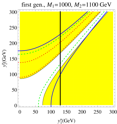
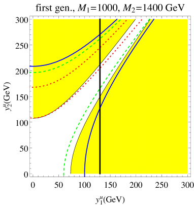
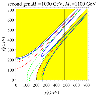
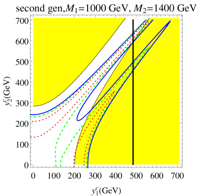
Figure 1: Tree level (yellow area is excluded at 3$\sigma$), EWPT (blue continuous line corresponds to the 3$\sigma$ bound, green dashed to 2$\sigma$, red dotted to 1$\sigma$, the strip between the lines is allowed) and LHC single VLQ production bounds (vertical black line, excluded region on the right) in the case of mixing of two VLQ multiplets with the first (top panels) or second (bottom panels) SM quark generation. Plots on the left column correspond to benchmark masses $M_{1}=1000$ GeV and $M_{2}=1100$ GeV, while on the right to $M_{1}=1000$ GeV and $M_{2}=1400$ GeV.

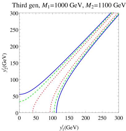
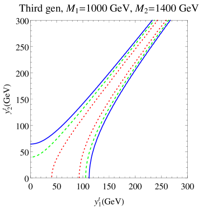
Figure 2: EWPT bounds (blue line is the 3$\sigma$ bound, green dashed 2$\sigma$, red dotted 1$\sigma$, the strip between the lines is allowed) in the case of mixing of the two VLQ multiplets with the third SM quark generation.

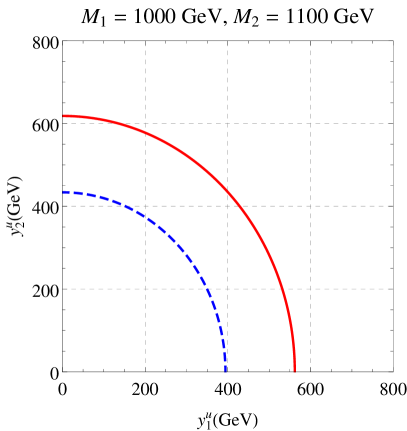
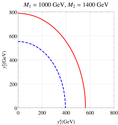
Figure 3: First generation mixing bounds from Higgs couplings data, Blue dotted line is 68% CL and Red line corresponds to 95% CL. Values of the Yukawa couplings below the corresponding curve are allowed.

A combination of the numerical results we obtained are shown in Figs. 1, 2 and 3 for a selection of benchmarks. The details of the bounds we impose are described in the following sub-sections 3.1 and 3.2. The general trend is that, for VLQs that couple mainly to the first and second SM quark families, the bounds from EWPTs (curved lines) and tree level $Z$-couplings (excluded yellow area) tend to cover the same parameter space. This was also remarked in Cacciapaglia:2015ixa , where the specific case of degenerate or quasi degenerate multiplets was considered. For earlier discussion of the degenerate case, we refer the reader to Refs Atre:2011ae ; Atre:2013ap . In the cases we cover here, with less degenerate masses, we see that the allowed region shifts in the parameter space of the two Yukawa couplings, while the approximate overlap between tree and loop level bounds is conserved. The vertical black line gives a constraint on the Yukawa coupling coming from direct searches for a VLQ bottom partner at the LHC Run-II (more details in the following sub-section 3.3). We remark that bounds also arise from modifications to the Higgs couplings, mainly due to loops of VLQs to the couplings to gluons and photons. However, such bounds (shown in Fig. 3) are much weaker and do not significantly affect the allowed parameter space.

The case of third generation is quite different, as there are no tree level bounds due to our poor knowledge of the couplings of the $Z$ boson to the top quark. Furthermore, the loop contribution to the Higgs coupling features an interesting cancellation, thus leading to very weak constraints. The loop level EWPTs, however, give similar constraints to the ones from light families, as shown in Fig. 2, and also features a characteristic shape due to a cancellation that allows large values of the couplings.

3.1 Tree level bounds

Among the long list of processes at tree level, we consider here only the most significant and effective one to obtain bounds on the parameters of VLQs. Specifically, we use bounds on the modifications to the Z couplings induced by the mixing between VLQs and SM quarks. The couplings of VLQs to gauge bosons are given in the appendix B of Cacciapaglia:2015ixa . In the models under consideration, only the mixing of top partners with up-type SM quarks will induce this type of effects. The diagonalisation of the mass matrix is obtained through two unitary matrices $V_{L}$ and $V_{R}$, defined by

$$M_{u}=V_{L}\cdot M_{u}^{diag}\cdot V_{R}^{\dagger}\,,$$ (7)

and the mass eigenstates can be obtained by rotating the flavour eigenstates with the same matrices:

$$\left(\begin{array}[]{c}u\\ c\\ t\\ t^{\prime}_{1}\\ t^{\prime}_{2}\end{array}\right)_{L/R}=V^{\dagger}_{L/R}\cdot\left(\begin{array}[]{c}u^{1}\\ u^{2}\\ u^{3}\\ U_{1}\\ U_{2}\end{array}\right)_{L/R}\,.$$ (8)

The above rotations modify the couplings of SM and VLQs with the gauge bosons, affecting in turn well measured processes, in particular observables involving the Z boson. The expressions of couplings of VLQs, SM quarks and the gauge bosons of the SM are provided in Appendix A.3. The modifications to the couplings with respect to the SM values are proportional to the $V_{L/R}^{4I}$ and the $V_{L/R}^{5I}$ elements of the mixing matrices, and we recall that for doublets larger mixing angles are obtained in the right-handed sector, while the ones in the left-handed sector are suppressed by the ratio between the SM quark mass and the VLQ masses Buchkremer:2013bha .

Strong constraints on the Z coupling with first generation SM quarks come from the weak charge measurement in atomic parity violation experiments Deandrea:1997wk ; Patrignani:2016xqp . The couplings of the Z to the second generation quarks were tested in detail at LEP ALEPH:2005ab :

$$g_{ZL}^{c}=0.3453\pm 0.0036\,,\quad g_{ZR}^{c}=-0.1580\pm 0.0051\,,\quad\mbox{corr.}=0.30\,.$$ (9)

We remark that the bounds shown in Figs 1 and 2 are calculated at 3$\sigma$. For couplings to the third generation, the $W_{tb}$ couplings were measured both at TeVatron and LHC. The value of $V_{tb}$ is affected by the mixing of the top with the VLQs in the left-handed sector:

$$|V_{tb}|^{2}=1-\sum_{K=4,5}|V_{L}^{K3}|^{2}\,.$$ (10)

A complete list of direct measurements and lower bounds on $V_{tb}$ can be found in Chiarelli:2013psr . Again for more detailed formulas we refer to Cacciapaglia:2015ixa . Numerically, the bound from $V_{tb}$ are rather weak and do not significantly affect the parameter space for heavy VLQs.

3.2 Electroweak precision tests and Higgs bounds

Electroweak precision measurements, or EWPT, are a standard tool to constrain physics beyond the SM. They can be used to constrain the parameters of VLQs Cacciapaglia:2010vn ; Chen:2017hak , but only under the strong hypothesis that, except for the considered contributions, other heavy particles decouple or give negligible contributions. Seen the level of precision in the measurement, this is a rather strong assumption and may strongly bias the applicability of the results to specific models. For this reason, in the following, we will consider the bounds from EWPTs as an indication and not as a general exclusion, contrary to the tree level bounds. The Higgs measurements are also entering a precision era and, already at present, give valuable information and limits on the possible extensions of the SM. Model of VLQs are no exception and looking to the Higgs data gives useful constraints Bizot:2015zaa . EWPT and Higgs couplings measurements give rather complementary bounds on the parameters space of VLQ models.

Bounds from EWPTs are usually given in term of the oblique parameters S and T, as defined in Refs Peskin:1990zt ; Peskin:1991sw . We have considered the following reference SM values: $m_{h,{\rm ref}}=125$ GeV, $m_{t,{\rm ref}}=173$ GeV and $m_{b,{\rm ref}}=4.2$ GeV. Taking $U=0$, as it is the case in the models under scrutiny, the experimental values for the $S$ and $T$ parameters are Baak:2014ora :

$$S=0.06\pm 0.09\,,\qquad T=0.10\pm 0.07\,,$$ (11)

where the correlation between $S$ and $T$ in this fit is 0.91. For more details and the complete list of formulas we refer to Cacciapaglia:2015ixa .

The EWPTs, complemented by the tree-level bounds for the light generations, tend to favour situations in which the two Yukawa couplings of the VLQ doublets to the SM are of similar size (see Figures 1 and 2), giving rise to a funnel region that extends to large value of the Yukawas along the diagonal. In the non-degenerate VLQ mass case, the funnel is simply rotated away from the exact diagonal, shifting closer to the axis relative to the heavier multiplet. This, as expected, derives from stronger bounds on the Yukawa of the lighter multiplet.

Concerning Higgs data, the direct measurement of the couplings to quarks is very challenging: only very recently the observation of production of the Higgs in association with tops has been reported by CMS ttH that measured the signal strength with a $30\%$ accuracy, while the couplings to light quarks (with the exception of the bottom) is out of reach. Thus, the only bounds come, indirectly, from loop effects on the couplings to gluons and photons. Being generated at loop level, they also suffer from the possible presence of additional contributions that would thus affect the bounds in more complete models. The combined ATLAS-CMS constraints on $\kappa_{\gamma}$ and $\kappa_{g}$ are given in Ref. exp_higgs . The presence of new VLQs, which enter the loops allowing the Higgs boson to couple to photons and gluons, modifies these effective couplings giving rise to bounds on the parameter space of VLQs. We use therefore those combined constraints in the following to establish bounds on the parameter space for VLQ bi–doublets as shown in Figure 3. These bound put an upper limit on the funnel region which was unrestricted by tree-level and EWPT data. The results of second generation mixing with VLQs are similar to those for the first generation mixing. On the contrary the third generation mixing case does not allow to put any extra constraint using the Higgs results.

3.3 Bounds from direct searches at the LHC

As we already pointed out, VLQs are widely searched for at the LHC. Most efforts, so far, have been addressed towards VLQs that decay into third generation quarks and are pair produced via QCD interactions. For a top partner, the considered final states are $Wb$, $Zt$ and $Ht$. In the case of doublets, the rate into the charged current is nearly negligible, thus leading to bounds ranging from $1270$ GeV to $1300$ GeV from the latest CMS results Sirunyan:2018omb ; Sirunyan:2017usq , while ATLAS Aaboud:2018xuw ; Aaboud:2017qpr gives $1170$ to $1430$ GeV. Interestingly, for CMS the stronger bound corresponds to decays exclusively into $Zt$, while for ATLAS into $tH$. For completeness, similar bounds can be obtained for decays into $Wb$ final states Sirunyan:2017pks ; Aaboud:2017zfn . The bounds on the charge $-1/3$ $B$ and charge $5/3$ X, which decay uniquely into $Wt$, range between $1100$ GeV (for same sign lepton channels) CMS-PAS-B2G-16-019 to $1300$ GeV (for single lepton channels) CMS-PAS-B2G-17-008 for CMS. In the approximations considered in the searches, those bounds do not depend on the value of the mixing angles with the SM quarks. Searches targeting single production channels, which are proportional to the mixing angles, are also available within the latest dataset. CMS has published a search for $B$ in the final state $Ht$ Sirunyan:2018fjh and for $T$ in the final state $Zt$ Sirunyan:2017ynj , while ATLAS has a search in $Wb$ for the 2015 dataset ATLAS-CONF-2016-072 . Only the search in the $Zt$ channel can, in principle, be used to set bounds on the Yukawa-like couplings in our model. However, we have checked that the cross sections we obtain are always smaller than the observed bounds.

Figure 4: Cross sections for single production of a bottom partner $B$ in $pp\to Bq$, as a function of the $y_{1}^{q}$ (in GeV) for first and second generation mixing. The mass is fixed to $1000$ GeV, and the cross sections are compared to the 95% CL bound from Sirunyan:2017lzl at 8 TeV (black horizontal line).

Fewer searches also cover the case of the couplings to light generations, and are limited to Run I data. From QCD pair production Sirunyan:2017lzl , the bounds range between $430$ GeV for exclusive decays into $Ht$ to $605$ for $Zt$. Thus, our benchmark points are well above the current exclusion. In this case, however, single production can be very important thanks to the couplings to valence quarks Atre:2011ae ; Buchkremer:2013bha . However, interpreting the bounds is more challenging, as they depend on the structure of the couplings to the light quarks that enter the single production. For the charge $2/3$ partners, in our case the dominant production is via the couplings to the $Z$, which is however not covered in the CMS analysis. Thus, the only bound we could directly apply to our scenario is for the single production of a bottom-type VLQ, $B$ in the SM-like multiplet, as cross-sections are bound by the limits for $pp\to Bq$ from the CMS analysis Sirunyan:2017lzl at 8 TeV. In turn this provides an upper bound on the maximal value of the Yukawa couplings for the SM-like doublet, $y_{1}^{u/c}$. To extract the bound, we have calculated the production cross section at LO, using the model implementation described in more details in Section 4.2, and compared it to the excluded value at 95% CL. Note that the mass of the $B$ VLQ is equal to $M_{1}$, which is fixed to $1000$ GeV in our benchmarks. The result is shown in Figure 4, where we compare the production cross section for couplings to up (in violet) and charm (in red) quarks to the exclusion limit at a cross section of $\sim 250$ fb. Note that we only consider the central value here, and that an increase of the cross section due to QCD NLO effects should be expected Fuks:2016ftf . Theoretical errors from scale variation are strongly reduced at NLO. The net bounds on $y_{1}^{u/c}$ amount to $y_{1}^{u}<130$ GeV and $y_{1}^{c}<485$ GeV, and they are shown as a black vertical line in Figure 1: the region on the left side of the line is allowed.

4 LHC phenomenology

Having determined the allowed region in parameter space, we now perform a phenomenological analysis of the signatures expected at the LHC. Compared to the current search strategies, which are based on simplified scenarios with a single VLQ, we will consider here in detail the interplay between the two VLQ doublets with hypercharges $Y=1/6$ and $Y=7/6$. We will show that peculiar patterns in the decay rates can be observed, as well as new production channels.

Among the key properties of this scenario is the presence of two top partners that mix and have different masses and decay patterns. One feature common to all top partners coming from doublets is that the decay via charged currents, i.e. a $W^{\pm}$ boson, are very suppressed, thus searches based on this decay channel (which give the strongest bounds) will be ineffective. As we will see, peculiar decay patterns may be used to effectively tag this kind of scenario.

4.1 Masses and branching ratios

The analytical expressions of the masses and branching ratios (BRs) are reported in Appendices A.2 and A.4 respectively. We recall that the values of the masses for $t^{\prime}_{1}$ and $t^{\prime}_{2}$ are not constant but depend on the values of the two Yukawas, as shown in Fig. 5. We show results for the light quarks and for the benchmark masses $M_{1}=1000$ GeV and $M_{2}=1200$ GeV. For mixing with the top, the results are qualitatively similar and quantitatively very close too, as the VLQ masses are already constrained to be much heavier that the top, as discussed in the previous section. On the other hand, the bottom-partner $B$ and exotic charged $X^{5/3}$ have masses fixed, respectively, to $M_{1}$ and $M_{2}$, and BRs of 100% into $B\to W^{-}u/c/t$ and $X^{5/3}\to W^{+}u/c/t$.

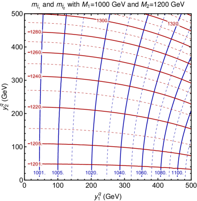
Figure 5: Masses in GeV of $t^{\prime}_{1}$ (blue contours) and $t^{\prime}_{2}$ (red contours) mixing with the light quarks, for the benchmark $M_{1}=1000$ GeV and $M_{2}=1200$ GeV. The contours are shown at intervals of 10 GeV unless specified. Results for mixing with the top quark are numerically almost identical.

For the branching ratios, in this section we present sample numerical results for the intermediate benchmark scenario with $M_{1}=1000$ GeV and $M_{2}=1200$ GeV, as the results for the other two cases as well as for heavier masses are qualitatively similar.

We start from the lighter top partner, $t_{1}^{\prime}$. In Fig. 6 we show contours of the BRs of a $t_{1}^{\prime}$ that mixes with the up quark. The contours are shown in the plane identified by the two Yukawa couplings. Results for mixing to the charm are nearly identical (differences only depend on the mass of the charm, which is much smaller that the VLQ masses), so we superimpose on the same plot the regions excluded by tree level constraints for the two cases: orange for the charm, with the pink area additionally excluded for the up. The orange line marks the additional portion of parameter space that would be excluded at 3$\sigma$ by the loop-level EWPTs, in absence of additional contribution from New Physics and for mixing to the charm (for the up, the tree level bounds are always dominant). We notice that the charged current is absent, and that the decay rates are mostly sensitive to the value of the Yukawa for the second multiplet. For small values of $y_{2}^{q}$, the rates are almost equal between $Z$ and Higgs, while at large values the $Z$ tends to dominate. The analogous BRs for mixing of $t^{\prime}_{1}$ to the top are numerically very similar, due to the smallness of the top mass compared to the VLQ ones while , however, the excluded region is different (recall the absence of tree-level constraints).

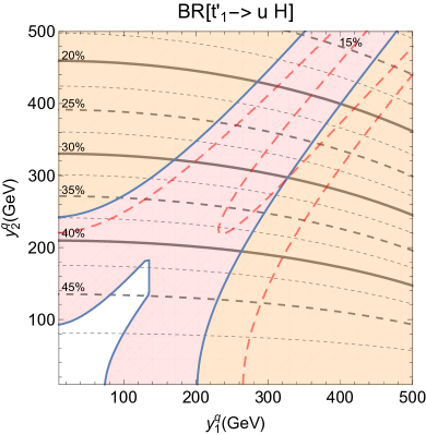
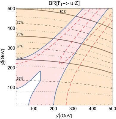
Figure 6: Branching ratios of $t_{1}^{\prime}$ mixing with the up/charm quark . The contours are show for values of the BR spaced by steps of $2.5\%$. For the light quarks, the orange region is excluded for the charm, while the orange plus pink areas are excluded for the up. The dashed line indicate the region excluded by EWPTs for mixing to the charm.

For the heavier $t_{2}^{\prime}$, we show the BRs in Figs 7 for couplings to light generations. We note the same pattern in the balance between the $Z$ and Higgs final states, but with inverted roles: it is the BR into the Higgs that dominates, in this case, for large values of the Yukawa with the first doublet, $y_{1}^{q}$. In addition, decays into the lighter VLQ $t^{\prime}_{1}$ are also allowed, but with very small rates that only increase above the few percent for large Yukawa couplings.

It is useful to remark that, for mixing to the up quark, the allowed parameter region is very small, thus the values of the BRs are constrained to almost fixed values. For both $t^{\prime}_{1}$ and $t^{\prime}_{2}$, the rates into $uZ$ and $uH$ are close to $50\%$, while decays $t^{\prime}_{2}\to t^{\prime}_{1}Z/H$ are always bound to be below $1\%$.

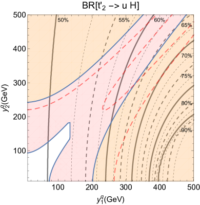
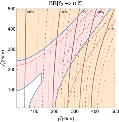
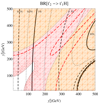
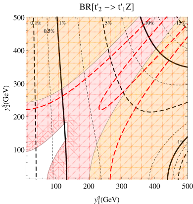
Figure 7: Branching ratios of $t_{2}^{\prime}$ mixing with the up/charm quark. The contours are show for values of the BR spaced by steps of $2.5\%$ (unless specified). The orange region is excluded for the charm, while the orange plus pink areas are excluded for the up. The dashed line indicate the region excluded by EWPTs for mixing to the charm.

4.2 Cross-sections

The production cross-sections at the LHC also show distinctive patterns. For the calculation, we have used a modified version of the Feynrules Alloul:2013bka VLQ model files provided in Ref. Fuks:2016ftf . A modification is necessary for including couplings between VLQs from different multiplets and SM gauge and Higgs bosons. Such modifications allow an estimation of processes where VLQs of different multiplets are produced in association, as $pp\to t_{1}^{\prime}t_{2}^{\prime}$. We have used Madgraph5 version 2.6.1 Alwall:2011uj for the estimation of cross-sections at LO in QCD, using the NN23LO1 parton distribution functions for the proton.

We computed the production cross-sections at 13 TeV for the production of the charge $2/3$ VLQs $t_{1,2}^{\prime}$ in the parameter space allowed by precision, low energy and LHC@8TeV constraints, determined in Section 3. We also focus on mixing to the up quark, which allows for sizeable single production rates thanks to the couplings to a valence quark in the proton. We chose, as representative benchmark, the set of input parameter $M_{1}=1000$ GeV and $M_{2}=1200$ GeV and scanned over the allowed values of the Yukawa couplings in the $y_{1}^{u}$ - $y_{2}^{u}$ plane. Specifically, we have considered processes of single production of $t_{1}^{\prime}$ and $t_{2}^{\prime}$ in association with SM objects, $pp\to t_{1,2}^{\prime}+\{h,Z,j\}$, and pair production of top partners of same or different kind, $pp\to t_{i}^{\prime}t_{j}^{\prime}$ with $i,j=1,2$, therefore including both QCD- and EW-strength couplings. In all cases we have considered both the production of particle and anti-particle states. Our results are summarised in Fig. 8.

Figure 8: Scatter plot of production cross-sections at LHC@13TeV, scanning over the Yukawa coupling of $t_{2}^{\prime}$, for the production processes (from top left clockwise): $t_{i}^{\prime}+h$, $t_{i}^{\prime}+Z$, $t_{i}^{\prime}t_{j}^{\prime}$ and $t_{i}^{\prime}+\text{jet}$ with $(i,j=1,2)$ and with $M_{1}=1000$ GeV and $M_{2}=1200$ GeV. The cross-section include also the production of the anti-particle states $\overline{t}_{i,j}^{\prime}$.

A number of conclusions can be derived:

• In the allowed region of parameter space, it is always possible to obtain configurations in which the production cross-section of the heavier VLQ ($t_{2}^{\prime}$) is comparable or even larger than the cross-section for the lighter VLQ ($t_{1}^{\prime}$). For single production channels, this switch happens for values of $y^{u}_{1}$ smaller than $60\div 80$ GeV, while for pair production channel the production of $t_{2}^{\prime}$ is comparable to $t_{1}^{\prime}$ for values of $y_{1}^{u}$ around the upper allowed limit. From a phenomenological point of view, this result can be very interesting because the decay patterns of the heavier top-partner are different from the ones usually considered in experimental searches. This includes the possibility of chain-decays to the lighter $t_{1}^{\prime}$, thus opening new channels for experimental exploration.

• The cross-section for production of a pair of VLQs of same kind exhibits an interesting pattern that indicates the dominance of EW production mechanism for large values of Yukawa couplings. In fact, QCD production only depends on the mass, which depends only mildly on the Yukawas. From the bottom-right plot in Fig.8, however, we see a marked increase in the cross-section of both VLQs for $y_{1}^{u}>60\div 80$ GeV. In addition, the pure electroweak production of the two VLQs together, $t_{1}^{\prime}t_{2}^{\prime}$, becomes sizeable in the same parameter region, and it even dominates over pair production for the largest allowed values of the Yukawa couplings. This may be extremely relevant for phenomenological analyses as the kinematics of processes of production of a pair of VLQ with different masses will be different from the one usually considered in experimental searches where the same VLQ is produced in pairs only through QCD-driven processes. A similar effect was noted in Ref. Cacciapaglia:2009cu for VLQs in the context of Little Higgs models with T-parity and, more recently, the same phenomena was noted in Brooijmans:2018xbu ; Fuks:2016ftf .

The results we highlighted show novel channels that deserve a thoroughly investigation, as they may give rise to detectable characteristic signatures at the LHC. Furthermore, an analysis at NLO in QCD Fuks:2016ftf ; Cacciapaglia:2017gzh is needed to go beyond a simple cross-section calculation, together with the addition of detector and reconstruction effects.

5 Conclusions

We have considered VLQs in a more general framework than the usual simplified models, namely we study the presence of two doublets with general mixing structure with the SM quark generations. This template, inspired by situations which are typically present in various NP models, shows that present bounds in the general case are weaker than those assuming a single VLQ multiplet and coupling only to the third SM quark generation. Moreover we focused on the two “top-partner-type” heavy VLQs present in the case of the two studied multiplets. Due to their peculiar mixing patterns with the SM quarks, they feature production and decay channels that are usually not considered in experimental searches. In particular, we remark areas in the parameter space for sizeable Yukawa couplings where the single production of the heavier partner dominates, thus leading to cascade decays. Furthermore, in the same parameter region, production of the two mass eigenstates in association can dominate over QCD and EW pair production. These new features deserve to be included within the exploration programs for NP at the LHC, thus allowing to test these situations in detail.

Appendix A Appendix

A.1 Multiplets

The doublets we consider allow to have mixing with the SM and one state with same quantum numbers in the two multiplets, and in the main text we focused on the situation in which each doublet contains a top-partner. However it is also possible to have two bottom partners, giving rise to the following two cases of either two $T^{\prime}$ VLQs or two $B^{\prime}$ VLQs.

Case 1) Doublet $Y=1/6$ and Doublet $Y=7/6$

In the case of two VLQ doublets, due to their quantum numbers, they couple to the right-handed SM quarks:

$$\mathcal{L}_{V-SM} = -\lambda_{1}^{k}\,\bar{\psi}_{1L}\tilde{H}u_{R}^{k}-\lambda_{1d}^{k}\,\bar{\psi}_{1L}Hd_{R}^{k}-\lambda_{2}^{k}\,\bar{\psi}_{2L}Hu_{R}^{k}+h.c.\,,$$ (12)

where the VLQ fermions are $\psi_{1}=({\bf 2},\frac{1}{6})=\left(U_{1}\ D_{1}\right)^{T}$ and $\psi_{2}=({\bf 2},\frac{7}{6})=\left(X_{2}^{5/3}\ U_{2}\right)^{T}$. No Yukawa coupling between the two VLQ multiplet is allowed, therefore one can use two free phases to remove one phase in $\lambda_{1}^{k}$ and one in $\lambda_{2}^{k}$ (therefore only four new phases are present). The mass Lagrangian is:

$$\mathcal{L}_{\rm mass} = -y_{1u}^{k}\bar{U}_{1L}u_{R}^{k}-y_{1d}^{k}\bar{D}_{1L}d_{R}^{k}-y_{2}^{k}U_{2L}u^{k}_{R}$$ (13)

$$-M_{1}\,\bar{U}_{1L}U_{1R}-M_{1}\,\bar{D}_{1L}D_{1R}-M_{2}\,\bar{U}_{2L}U_{2R}-M_{2}\,\bar{X}^{5/3}_{2L}X^{5/3}_{2R}+h.c.\,,$$

and mass matrices are:

$$M_{u}=\left(\begin{array}[]{c c c}\left(\tilde{m}^{up}\right)_{3\times 3}&0_{3\times 1}&0_{3\times 1}\\ (y_{1u}^{k})_{1\times 3}&M_{1}&0\\ (y_{2}^{k})_{1\times 3}&0&M_{2}\end{array}\right),\quad M_{d}=\left(\begin{array}[]{c c }\left(\tilde{m}^{down}\right)_{3\times 3}&0_{3\times 1}\\ (y_{1d}^{k})_{1\times 3}&M_{1}\\ \end{array}\right),\quad M_{X^{5/3}}=M_{2}\,.$$ (14)

Case 2) Doublet $Y=1/6$ and Doublet $Y=-5/6$

We have not considered in the main text the case of two bottom partners as it requires a different study, implying also the use of quite different bounds. We give it here for completeness and future reference for further studies. In this case the the Lagrangian $\mathcal{L}_{V-SM}$ differs from the one of the previous case due to the different weak hypercharge of the second doublet:

$$\mathcal{L}_{V-SM}=-\lambda_{1}^{k}\,\bar{\psi}_{1L}\tilde{H}u_{R}^{k}-\lambda_{1d}^{k}\,\bar{\psi}_{1L}Hd_{R}^{k}-\lambda_{2d}^{k}\bar{\psi_{2}}_{L}\tilde{H}d^{k}_{R}+h.c.\,,$$ (15)

where the VLQ fermions are $\psi_{1}=({\bf 2},\frac{1}{6})=\left(U_{1},D_{1}\right)^{T}$ and $\psi_{2}=({\bf 2},-\frac{5}{6})=\left(D_{2},Y_{2}^{-4/3}\right)^{T}$. The mass Lagrangian is:

$$\mathcal{L}_{\rm mass} = -y_{1}^{k}\bar{U}_{1L}u_{R}^{k}-y_{1d}^{k}\bar{D}_{1L}d_{R}^{k}-y_{2d}^{k}\bar{D}_{2L}d_{R}^{k}-M_{1}\,\bar{U}_{1L}U_{1R}-M_{1}\,\bar{D}_{1L}D_{1R}$$ (16)

$$-M_{2}\,\bar{D}_{2L}D_{2R}-M_{2}\,\bar{Y}^{-4/3}_{2L}Y^{-4/3}_{2R}+h.c.\,,$$

and mass matrices are:

$$M_{u}=\left(\begin{array}[]{cc}\left(\tilde{m}^{up}\right)_{3\times 3}&0_{3\times 1}\\ (y_{1}^{k})_{1\times 3}&M_{1}\end{array}\right)\,,\quad M_{d}=\left(\begin{array}[]{c c c}\left(\tilde{m}^{down}\right)_{3\times 3}&0_{3\times 1}&0_{3\times 1}\\ (y_{1d}^{k})_{1\times 3}&M_{1}&0\\ (y_{2d}^{k})_{1\times 3}&0&M_{2}\end{array}\right)\,,\quad M_{Y^{-4/3}}=M_{2}\,.$$ (17)

A.2 Masses

In the top-type bi-doublet case we consider, both VLQ multiplets only couple to the right-handed SM quarks:

$$\mathcal{L}_{V-SM} = -\lambda_{1}^{k}\,\bar{\psi}_{1L}\tilde{H}u_{R}^{k}-\lambda_{1d}^{k}\,\bar{\psi}_{1L}Hd_{R}^{k}-\lambda_{2}^{k}\,\bar{\psi}_{2L}Hu_{R}^{k}+h.c.\,,$$ (18)

where $\psi_{1}=({\bf 2},\frac{1}{6})=\left(U_{1}\ D_{1}\right)^{T}$ and $\psi_{2}=({\bf 2},\frac{7}{6})=\left(X_{2}^{5/3}\ U_{2}\right)^{T}$. In this case, no Yukawa coupling between the two VLQ multiplet is allowed, therefore one can use the two free phases to remove one phase in $\lambda_{1}^{k}$ and one in $\lambda_{2}^{k}$, so that only 4 new phases are present in this model. Once again, we will set $\lambda_{1d}^{k}=0$. The mass Lagrangian and mass matrices become:

$$\mathcal{L}_{\rm mass} = -y_{1u}^{k}\bar{U}_{1L}u_{R}^{k}-y_{1d}^{k}\bar{D}_{1L}d_{R}^{k}-y_{2}^{k}U_{2L}u^{k}_{R}$$ (19)

$$-M_{1}\,\bar{U}_{1L}U_{1R}-M_{1}\,\bar{D}_{1L}D_{1R}-M_{2}\,\bar{U}_{2L}U_{2R}-M_{2}\,\bar{X}^{5/3}_{2L}X^{5/3}_{2R}+h.c.\,,$$

and

$$M_{u}=\left(\begin{array}[]{c c c}\left(\tilde{m}^{up}\right)_{3\times 3}&0_{3\times 1}&0_{3\times 1}\\ (y_{1}^{k})_{1\times 3}&M_{1}&0\\ (y_{2}^{k})_{1\times 3}&0&M_{2}\end{array}\right),\quad M_{d}=\left(\begin{array}[]{c c }\left(\tilde{m}^{down}\right)_{3\times 3}&0_{3\times 1}\\ (0)_{1\times 3}&M_{2}\\ \end{array}\right),\quad M_{X^{5/3}}=M_{2}\,.$$ (20)

The masses of $B^{\prime}$ and $X^{5/3}$ are:

$$m_{b^{\prime}} = M_{2}\,,$$ (21)

$$m_{X^{5/3}} = M_{2}\,.$$ (22)

We define the dimensionless $X$ and $Y$ parameters as

$$X=\frac{(y_{1}^{k})^{2}}{M_{1}^{2}-m_{k}^{2}}\,,\quad Y=\frac{(y_{2}^{k})^{2}}{M_{2}^{2}-m_{k}^{2}}\,,$$ (23)

where $k=u,c,t$. In the bi-doublet model, the top Yukawa coupling and masses of heavy top partners can be written as

$$\tilde{m}_{t}^{2} = m_{t}^{2}\left(1+X+Y\right)\,,$$ (24)

$$m_{t^{\prime}_{1}}^{2} = m_{t^{\prime}}^{2}-\frac{\Delta m_{t^{\prime}}^{2}}{2}\,,$$ (25)

$$m_{t^{\prime}_{2}}^{2} = m_{t^{\prime}}^{2}+\frac{\Delta m_{t^{\prime}}^{2}}{2}\,,$$ (26)

with

$$m_{t^{\prime}}^{2} = \frac{M_{1}^{2}(1+X)+M_{2}^{2}(1+Y)}{2}\,,$$ (27)

$$\Delta m_{t^{\prime}}^{2} = 2\sqrt{m_{t^{\prime}}^{4}-M_{1}^{2}M_{2}^{2}\frac{\tilde{m}_{t}^{2}}{m_{t}^{2}}}\,.$$ (28)

For $M_{1}=M_{2}=M$, these can be written as

$$\tilde{m}_{t}^{2} = m_{t}^{2}\left(1+\frac{(y_{1}^{t})^{2}+(y_{2}^{t})^{2}}{M^{2}-m_{t}^{2}}\right)\,,$$ (29)

$$m_{t^{\prime}_{1}}^{2} = M^{2}\,,$$ (30)

$$m_{t^{\prime}_{2}}^{2} = M^{2}\left(1+\frac{(y_{1}^{t})^{2}+(y_{2}^{t})^{2}}{M^{2}-m_{t}^{2}}\right)\,.$$ (31)

If $M\gg y_{1}^{t},y_{2}^{t}$:

$$\tilde{m}_{t}^{2} = m_{t}^{2}\left(1+\frac{(y_{1}^{t})^{2}+(y_{2}^{t})^{2}}{M^{2}}\right)+{\cal O}\left(\frac{1}{M^{4}}\right)\,,$$ (32)

$$\Delta m_{t^{\prime}}^{2} = ((y_{1}^{t})^{2}+(y_{2}^{t})^{2})\left(1+\frac{m_{t}^{2}}{M^{2}}\right)+{\cal O}\left(\frac{1}{M^{4}}\right)\,.$$ (33)

As we showed in the main text, after imposing precision and low energy constraints in the parameter space of Yukawa couplings, a diagonal band is allowed by both the constraints even for large Yukawa couplings. When the gauge eigenstate masses of VLQ T-quarks are degenerate (i.e. $M_{1}=M_{2}$) then $BR(t_{1}^{\prime}\to qZ)=100\%$. This changes when VLT quarks are non-degenerate.

A.3 Couplings to gauge bosons

In the gauge basis, the general expressions for the couplings of $W^{\pm}$ bosons in the two VLQ multiplets models are given by

$$\mathcal{L}_{W^{\pm}} = \frac{g}{\sqrt{2}}\left(\begin{array}[]{ccccc}\bar{u}_{L}^{1},&\bar{u}_{L}^{2},&\bar{u}_{L}^{3},&\bar{U}_{1L},&\bar{U}_{2L}\\ \end{array}\right)\cdot\delta_{L}\cdot\gamma^{\mu}\left(\begin{array}[]{c}d_{L}^{1}\\ d_{L}^{2}\\ d_{L}^{3}\\ D_{1L}\\ D_{2L}\\ \end{array}\right)W_{\mu}^{+}$$ (40)

$$+ \frac{g}{\sqrt{2}}\left(\begin{array}[]{ccccc}\bar{u}_{R}^{1},&\bar{u}_{R}^{2},&\bar{u}_{R}^{3},&\bar{U}_{1R},&\bar{U}_{2R}\\ \end{array}\right)\cdot\delta_{R}\cdot\gamma^{\mu}\left(\begin{array}[]{c}d_{R}^{1}\\ d_{R}^{2}\\ d_{R}^{3}\\ D_{1R}\\ D_{2R}\\ \end{array}\right)W_{\mu}^{+}+h.c.\,,$$ (47)

with

$$\delta_{L}=\left(\begin{array}[]{ccc}I_{3\times 3}&&\\ &\alpha_{1}&\\ &&\alpha_{2}\\ \end{array}\right)\,,\quad\delta_{R}=\left(\begin{array}[]{ccc}0_{3\times 3}&&\\ &\alpha_{1}&\\ &&\alpha_{2}\\ \end{array}\right)\,,$$ (48)

where the values for the $\alpha_{i}$ coefficients are reported in Table 5 of Ref. Cacciapaglia:2015ixa . In the mass basis, the left- and right-handed couplings can be written as

$$g_{WL}^{IJ} = \frac{g}{\sqrt{2}}V_{CKM}^{L,IJ}=\frac{g}{\sqrt{2}}V_{L}^{u\dagger}\cdot\delta_{L}\cdot V_{L}^{d}\,,$$ (49)

$$g_{WR}^{IJ} = \frac{g}{\sqrt{2}}V_{CKM}^{R,IJ}=\frac{g}{\sqrt{2}}V_{R}^{u\dagger}\cdot\delta_{R}\cdot V_{R}^{d}\,,$$ (50)

where $V_{CKM}^{L}$ and $V_{CKM}^{R}$ are the left- and right-handed CKM matrix, respectively and $V_{L,R}$ are the mixing matrices in the left- and right-handed sectors respectively.

The general expression for the left-handed couplings of the $Z$ in the up quark sector can be written as:

$$\mathcal{L}_{Z}=\frac{g}{c_{W}}\,\left(\bar{u}_{L}^{1},\bar{u}_{L}^{2},\bar{u}_{L}^{3},\bar{U}_{1L},\bar{U}_{2L}\right)\cdot\left[\left(\frac{1}{2}-Q_{u}s_{W}^{2}\right)I_{5\times 5}-\Delta T_{3}^{(up)}\right]\gamma^{\mu}\cdot\left(\begin{array}[]{c}u_{L}^{1}\\ u_{L}^{2}\\ u_{L}^{3}\\ U_{1L}\\ U_{2L}\end{array}\right)Z_{\mu}\,,$$ (51)

with:

$$\Delta T_{3}^{(up)}=\left(\begin{array}[]{ccc}0_{3\times 3}&&\\ &\Delta T_{3}^{(1,u)}&\\ &&\Delta T_{3}^{(2,u)}\\ \end{array}\right)\,,$$ (52)

where $I_{5\times 5}$ is the $5\times 5$ unit matrix and $\Delta T_{3}^{(k,u)}=1/2-T_{3}^{(k,u)}$ is the differences between the SM top-type quark and $k$-th generation VLQ. In the mass eigenstate basis, the left-handed coupling becomes:

$$g_{ZL}^{u,IJ}=\frac{g}{c_{W}}\left[\left(\frac{1}{2}-Q_{u}s^{2}_{W}\right)\delta^{IJ}-\sum_{k=1,2}\Delta T_{3}^{(k,u)}\left(V_{L}^{u*}\right)^{k+3,I}\left(V_{L}^{u}\right)^{k+3,J}\right]\,.$$ (53)

Analogously for the right-handed couplings we obtain:

$$g_{ZR}^{u,IJ}=\frac{g}{c_{W}}\left[\left(-Q_{u}s^{2}_{W}\right)\delta^{IJ}+\sum_{k=1,2}T_{3}^{(k,u)}\left(V_{R}^{u*}\right)^{k+3,I}\left(V_{R}^{u}\right)^{k+3,J}\right]\,.$$ (54)

In the interaction basis, the Yukawa interactions in top-type quarks can be written as:

$$\mathcal{L}_{H}=\frac{1}{v}\,\left(\bar{u}_{L}^{1},\bar{u}_{L}^{2},\bar{u}_{L}^{3},\bar{U}_{1L},\bar{U}_{2L}\right)\cdot\left[M_{u}-M\right]\cdot\left(\begin{array}[]{c}u_{R}^{1}\\ u_{R}^{2}\\ u_{R}^{3}\\ U_{1R}\\ U_{2R}\end{array}\right)h+h.c.\,,$$ (55)

with:

$$M=\left(\begin{array}[]{ccc}0_{3\times 3}&&\\ &M_{1}&\\ &&M_{2}\end{array}\right)\,.$$ (56)

In the mass eigenstate basis the coupling of top-type quark reads :

$$C_{L}^{u,IJ} = \frac{M_{u}^{diag,IJ}}{v}-\sum_{k=1,2}\frac{M_{k}}{v}\left(V_{R}^{u*}\right)^{k+3,I}\left(V_{L}^{u}\right)^{k+3,J}\,,$$ (57)

$$C_{R}^{u,IJ} = \frac{M_{u}^{diag,IJ}}{v}-\sum_{k=1,2}\frac{M_{k}}{v}\left(V_{L}^{u*}\right)^{k+3,I}\left(V_{R}^{u}\right)^{k+3,J}\,.$$ (58)

For bottom-type quark, we obtain:

$$C_{L}^{d,IJ} = \frac{M_{d}^{diag,IJ}}{v}-\sum_{k=1,2}\frac{M_{k}}{v}\left(V_{R}^{d*}\right)^{k+3,I}\left(V_{L}^{d}\right)^{k+3,J}\,,$$ (59)

$$C_{R}^{d,IJ} = \frac{M_{d}^{diag,IJ}}{v}-\sum_{k=1,2}\frac{M_{k}}{v}\left(V_{L}^{d*}\right)^{k+3,I}\left(V_{R}^{d}\right)^{k+3,J}\,.$$ (60)

A.4 Branching ratios

In the top-type bi-doublet case we consider, the VLQ $t^{\prime}_{1}$ and $t^{\prime}_{2}$ ($u_{I=4}$ and $u_{I=5}$) can decay at tree level to $d_{J}W^{+}$ and $X^{5/3}W^{-}$ via a charged current and to $Zu_{J}$ and $hu_{J}$ via a neutral current. The $u_{I}\to d_{J}W^{+}$ transition matrix element is given by

$${\cal M}=\bar{d}_{J}(q_{1})\gamma^{\mu}\left((g_{WL}^{JI})^{*}L+(g_{WR}^{JI})^{*}R\right)u_{I}(q_{2})\epsilon_{\mu}(\lambda)\,,$$ (61)

where $L$ and $R$ are the left- and right-handed projection operators. The partial width of $u_{I}\to d_{J}W^{+}$ decay is expressed as

$$\Gamma(u_{I}\to d_{J}W^{+}) = \frac{\lambda^{\frac{1}{2}}(1,m_{d_{J}}^{2}/m_{u_{I}}^{2},m_{W}^{2}/m_{u_{I}}^{2})}{32\pi m_{u_{I}}}$$ (62)

$$\Biggl{\{}\left(|g_{WL}^{JI}|^{2}+|g_{WR}^{JI}|^{2}\right)\left[m_{u_{I}}^{2}+m_{d_{J}}^{2}-2m_{W}^{2}+\frac{(m_{u_{I}}^{2}-m_{d_{J}}^{2})^{2}}{m_{W}^{2}}\right]$$

$$-12\left({\rm Re}g_{WL}^{JI}{\rm Re}g_{WR}^{JI}+{\rm Im}g_{WL}^{JI}{\rm Im}g_{WR}^{JI}\right)m_{u_{I}}m_{d_{J}}\Biggr{\}}\,,$$

where $I=4,5$ and $J=1,\cdots,4$, $\lambda(a,b,c)=a^{2}+b^{2}+c^{2}-2ab-2ac-2bc$ is the phase space function, and ${\rm Re}$ and ${\rm Im}$ indicate the real and imaginary part, respectively.

The $u_{I}\to X^{5/3}W^{-}$ transition matrix element is given by

$${\cal M}=\bar{X}^{5/3}(q_{1})\gamma^{\mu}\left(g_{WL}^{X^{5/3},I5}L+g_{WR}^{X^{5/3},I5}R\right)u_{I}(q_{2})\epsilon_{\mu}(\lambda)\,,$$ (63)

where $g_{WL}^{X^{5/3},I5}$ and $g_{WR}^{X^{5/3},I5}$ are the left- and right-handed couplings of $X^{5/3}$ given in Ref. Cacciapaglia:2015ixa . The partial width of $u_{I}\to X^{5/3}W^{-}$ decay is expressed as

$$\Gamma(u_{I}\to X^{5/3}W^{-}) = \frac{\lambda^{\frac{1}{2}}(1,m_{X^{5/3}}^{2}/m_{u_{I}}^{2},m_{W}^{2}/m_{u_{I}}^{2})}{32\pi m_{u_{I}}}$$ (64)

$$\Biggl{\{}\left(|g_{WL}^{X^{5/3},I5}|^{2}+|g_{WR}^{X^{5/3},I5}|^{2}\right)\left[m_{u_{I}}^{2}+m_{X^{5/3}}^{2}-2m_{W}^{2}+\frac{\left(m_{u_{I}}^{2}-m_{X^{5/3}}^{2}\right)^{2}}{m_{W}^{2}}\right]$$

$$-12\left({\rm Re}g_{WL}^{X^{5/3},I5}{\rm Re}g_{WR}^{X^{5/3},I5}+{\rm Im}g_{WL}^{X^{5/3},I5}{\rm Im}g_{WR}^{X^{5/3},I5}\right)m_{u_{I}}m_{X^{5/3}}\Biggr{\}}\,.$$

Concerning neural currents, the $u_{I}\to u_{J}Z$ transition matrix element is written as

$${\cal M}=\bar{u}_{J}(q_{1})\gamma^{\mu}\left(g_{ZL}^{u,IJ}L+g_{ZR}^{u,IJ}R\right)u_{I}(q_{2})\epsilon_{\mu}(\lambda)\,.$$ (65)

The partial width of $u_{I}\to u_{J}Z$ is

$$\Gamma(u_{I}\to u_{J}Z) = \frac{\lambda^{\frac{1}{2}}(1,m_{u_{J}}^{2}/m_{u_{I}}^{2},m_{Z}^{2}/m_{u_{I}}^{2})}{32\pi m_{u_{I}}}$$ (66)

$$\Biggl{\{}\left(|g_{ZL}^{u,IJ}|^{2}+|g_{ZR}^{u,IJ}|^{2}\right)\left[m_{u_{I}}^{2}+m_{u_{J}}^{2}-2m_{Z}^{2}+\frac{(m_{u_{I}}^{2}-m_{u_{J}}^{2})^{2}}{m_{Z}^{2}}\right]$$

$$-12\left({\rm Re}g_{ZL}^{u,IJ}{\rm Re}g_{ZR}^{u,IJ}+{\rm Im}g_{ZL}^{u,IJ}{\rm Im}g_{ZR}^{u,IJ}\right)m_{u_{I}}m_{u_{J}}\Biggr{\}}\,,$$

where $I=4,5$ and $J=1,2,\cdots<I$.

The matrix element of $u_{I}\to u_{J}h$ is written as

$${\cal M}=\bar{u}_{J}(q_{1})\left(C_{L}^{u,IJ}L+C_{R}^{u,IJ}R\right)u_{I}(q_{2})\,.$$ (67)

The partial width of $u_{I}\to u_{J}h$

$$\Gamma(u_{I}\to u_{J}h) = \frac{\lambda^{\frac{1}{2}}(1,m_{u_{J}}^{2}/m_{u_{I}}^{2},m_{h}^{2}/m_{u_{I}}^{2})}{32\pi m_{u_{I}}}$$ (68)

$$\Biggl{[}(m_{u_{I}}^{2}+m_{u_{J}}^{2}-m_{h}^{2})\left(|C_{L}^{u,IJ}|^{2}+|C_{R}^{u,IJ}|^{2}\right)+4m_{u_{I}}m_{u_{J}}\left({\rm Re}C_{L}^{u,IJ}{\rm Re}C_{R}^{u,IJ}\right.$$

$$\left.+{\rm Im}C_{L}^{u,IJ}{\rm Im}C_{R}^{u,IJ}\right)\Biggr{]}\,,$$

where $I=4,5$ and $J=1,2,\cdots<I$.

The total decay width of $u_{I}$ is given by

$$\Gamma_{total}(u_{I}) = \Gamma(u_{I}\to X^{5/3}W^{-})+\sum_{J=1}^{4}\Gamma(u_{I}\to d_{J}W^{+})$$ (69)

$$+\sum_{I>J}\left(\Gamma(u_{I}\to u_{J}Z)+\Gamma(u_{I}\to u_{J}h)\right)\,.$$

References

- (1) K. Agashe, R. Contino and A. Pomarol, The Minimal composite Higgs model, Nucl.Phys. B719 (2005) 165 [hep-ph/0412089].
- (2) R. Contino, L. Da Rold and A. Pomarol, Light custodians in natural composite Higgs models, Phys.Rev. D75 (2007) 055014 [hep-ph/0612048].
- (3) G. Giudice, C. Grojean, A. Pomarol and R. Rattazzi, The Strongly-Interacting Light Higgs, JHEP 0706 (2007) 045 [hep-ph/0703164].
- (4) O. Matsedonskyi, G. Panico and A. Wulzer, Light Top Partners for a Light Composite Higgs, JHEP 1301 (2013) 164 [1204.6333].
- (5) I. Antoniadis, A Possible new dimension at a few TeV, Phys.Lett. B246 (1990) 377.
- (6) I. Antoniadis, K. Benakli and M. Quiros, Finite Higgs mass without supersymmetry, New J.Phys. 3 (2001) 20 [hep-th/0108005].
- (7) C. Csaki, C. Grojean, J. Hubisz, Y. Shirman and J. Terning, Fermions on an interval: Quark and lepton masses without a Higgs, Phys.Rev. D70 (2004) 015012 [hep-ph/0310355].
- (8) Y. Hosotani, S. Noda and K. Takenaga, Dynamical gauge-Higgs unification in the electroweak theory, Phys.Lett. B607 (2005) 276 [hep-ph/0410193].
- (9) G. Cacciapaglia, A. Deandrea and J. Llodra-Perez, A Dark Matter candidate from Lorentz Invariance in 6D, JHEP 1003 (2010) 083 [0907.4993].
- (10) Y. Hosotani, Dynamical Mass Generation by Compact Extra Dimensions, Phys.Lett. B126 (1983) 309.
- (11) D. Choudhury, T. M. Tait and C. Wagner, Beautiful mirrors and precision electroweak data, Phys.Rev. D65 (2002) 053002 [hep-ph/0109097].
- (12) G. Panico, E. Ponton, J. Santiago and M. Serone, Dark Matter and Electroweak Symmetry Breaking in Models with Warped Extra Dimensions, Phys.Rev. D77 (2008) 115012 [0801.1645].
- (13) N. Arkani-Hamed, A. Cohen, E. Katz, A. Nelson, T. Gregoire et al., The Minimal moose for a little Higgs, JHEP 0208 (2002) 021 [hep-ph/0206020].
- (14) N. Arkani-Hamed, A. Cohen, E. Katz and A. Nelson, The Littlest Higgs, JHEP 0207 (2002) 034 [hep-ph/0206021].
- (15) M. Schmaltz and D. Tucker-Smith, Little Higgs review, Ann.Rev.Nucl.Part.Sci. 55 (2005) 229 [hep-ph/0502182].
- (16) K. Agashe, R. Contino, L. Da Rold and A. Pomarol, A Custodial symmetry for Zb anti-b, Phys.Lett. B641 (2006) 62 [hep-ph/0605341].
- (17) R. S. Chivukula, R. Foadi and E. H. Simmons, Patterns of Custodial Isospin Violation from a Composite Top, Phys.Rev. D84 (2011) 035026 [1105.5437].
- (18) F. del Aguila, M. Perez-Victoria and J. Santiago, Observable contributions of new exotic quarks to quark mixing, JHEP 09 (2000) 011 [hep-ph/0007316].
- (19) J. Aguilar-Saavedra, Pair production of heavy Q = 2/3 singlets at LHC, Phys.Lett. B625 (2005) 234 [hep-ph/0506187].
- (20) C. Anastasiou, E. Furlan and J. Santiago, Realistic Composite Higgs Models, Phys.Rev. D79 (2009) 075003 [0901.2117].
- (21) J. Aguilar-Saavedra, Identifying top partners at LHC, JHEP 0911 (2009) 030 [0907.3155].
- (22) G. Cacciapaglia, A. Deandrea, D. Harada and Y. Okada, Bounds and Decays of New Heavy Vector-like Top Partners, JHEP 1011 (2010) 159 [1007.2933].
- (23) D. Marzocca, M. Serone and J. Shu, General Composite Higgs Models, JHEP 1208 (2012) 013 [1205.0770].
- (24) A. De Simone, O. Matsedonskyi, R. Rattazzi and A. Wulzer, A First Top Partner Hunter’s Guide, JHEP 1304 (2013) 004 [1211.5663].
- (25) A. Falkowski, D. M. Straub and A. Vicente, Vector-like leptons: Higgs decays and collider phenomenology, JHEP 1405 (2014) 092 [1312.5329].
- (26) J. Aguilar-Saavedra, Mixing with vector-like quarks: constraints and expectations, EPJ Web Conf. 60 (2013) 16012 [1306.4432].
- (27) S. A. Ellis, R. M. Godbole, S. Gopalakrishna and J. D. Wells, Survey of vector-like fermion extensions of the Standard Model and their phenomenological implications, JHEP 1409 (2014) 130 [1404.4398].
- (28) A. Atre, G. Azuelos, M. Carena, T. Han, E. Ozcan, J. Santiago et al., Model-Independent Searches for New Quarks at the LHC, JHEP 08 (2011) 080 [1102.1987].
- (29) G. Cacciapaglia, A. Deandrea, L. Panizzi, N. Gaur, D. Harada et al., Heavy Vector-like Top Partners at the LHC and flavour constraints, JHEP 1203 (2012) 070 [1108.6329].
- (30) Y. Okada and L. Panizzi, LHC signatures of vector-like quarks, Adv.High Energy Phys. 2013 (2013) 364936 [1207.5607].
- (31) M. Buchkremer, G. Cacciapaglia, A. Deandrea and L. Panizzi, Model Independent Framework for Searches of Top Partners, Nucl.Phys. B876 (2013) 376 [1305.4172].
- (32) C. Delaunay, T. Flacke, J. Gonzalez-Fraile, S. J. Lee, G. Panico et al., Light Non-degenerate Composite Partners at the LHC, 1311.2072.
- (33) D. Barducci, A. Belyaev, M. Buchkremer, G. Cacciapaglia, A. Deandrea et al., Model Independent Framework for Analysis of Scenarios with Multiple Heavy Extra Quarks, 1405.0737.
- (34) ATLAS collaboration, G. Aad et al., Search for heavy vector-like quarks coupling to light quarks in proton-proton collisions at TeV with the ATLAS detector, Phys. Lett. B712 (2012) 22 [1112.5755].
- (35) CMS collaboration, A. M. Sirunyan et al., Search for vectorlike light-flavor quark partners in proton-proton collisions at =8 TeV, Phys. Rev. D97 (2018) 072008 [1708.02510].
- (36) J. Serra, Beyond the Minimal Top Partner Decay, JHEP 09 (2015) 176 [1506.05110].
- (37) G. Brooijmans et al., Les Houches 2015: Physics at TeV colliders - new physics working group report, in 9th Les Houches Workshop on Physics at TeV Colliders (PhysTeV 2015) Les Houches, France, June 1-19, 2015, 2016, 1605.02684, http://inspirehep.net/record/1456803/files/arXiv:1605.02684.pdf.
- (38) J. A. Aguilar-Saavedra, D. E. Lopez-Fogliani and C. Munoz, Novel signatures for vector-like quarks, JHEP 06 (2017) 095 [1705.02526].
- (39) M. Chala, Direct bounds on heavy toplike quarks with standard and exotic decays, Phys. Rev. D96 (2017) 015028 [1705.03013].
- (40) N. Bizot, G. Cacciapaglia and T. Flacke, Common exotic decays of top partners, 1803.00021.
- (41) A. Anandakrishnan, J. H. Collins, M. Farina, E. Kuflik and M. Perelstein, Odd Top Partners at the LHC, Phys. Rev. D93 (2016) 075009 [1506.05130].
- (42) S. Kraml, U. Laa, L. Panizzi and H. Prager, Scalar versus fermionic top partner interpretations of searches at the LHC, JHEP 11 (2016) 107 [1607.02050].
- (43) S. Moretti, D. O’Brien, L. Panizzi and H. Prager, Production of extra quarks decaying to Dark Matter beyond the Narrow Width Approximation at the LHC, Phys. Rev. D96 (2017) 035033 [1705.07675].
- (44) R. Balkin, M. Ruhdorfer, E. Salvioni and A. Weiler, Charged Composite Scalar Dark Matter, JHEP 11 (2017) 094 [1707.07685].
- (45) M. Chala, R. Gröber and M. Spannowsky, Searches for vector-like quarks at future colliders and implications for composite Higgs models with dark matter, JHEP 03 (2018) 040 [1801.06537].
- (46) G. Cacciapaglia, A. Deandrea, N. Gaur, D. Harada, Y. Okada and L. Panizzi, Interplay of vector-like top partner multiplets in a realistic mixing set-up, JHEP 09 (2015) 012 [1502.00370].
- (47) G. Cacciapaglia, S. R. Choudhury, A. Deandrea, N. Gaur and M. Klasen, Dileptonic signatures of T-odd quarks at the LHC, JHEP 03 (2010) 059 [0911.4630].
- (48) F. del Aguila and M. J. Bowick, The Possibility of New Fermions With I = 0 Mass, Nucl.Phys. B224 (1983) 107.
- (49) D. B. Kaplan, Flavor at SSC energies: A New mechanism for dynamically generated fermion masses, Nucl.Phys. B365 (1991) 259.
- (50) H. Georgi and D. B. Kaplan, Composite Higgs and Custodial SU(2), Phys. Lett. 145B (1984) 216.
- (51) G. Cacciapaglia, H. Cai, T. Flacke, S. J. Lee, A. Parolini and H. Serôdio, Anarchic Yukawas and top partial compositeness: the flavour of a successful marriage, JHEP 06 (2015) 085 [1501.03818].
- (52) G. Panico, M. Redi, A. Tesi and A. Wulzer, On the Tuning and the Mass of the Composite Higgs, JHEP 1303 (2013) 051 [1210.7114].
- (53) C.-Y. Chen, S. Dawson and E. Furlan, Vectorlike fermions and Higgs effective field theory revisited, Phys. Rev. D96 (2017) 015006 [1703.06134].
- (54) N. Bizot and M. Frigerio, Fermionic extensions of the Standard Model in light of the Higgs couplings, JHEP 01 (2016) 036 [1508.01645].
- (55) A. Atre, M. Chala and J. Santiago, Searches for New Vector Like Quarks: Higgs Channels, JHEP 1305 (2013) 099 [1302.0270].
- (56) A. Deandrea, Atomic parity violation in cesium and implications for new physics, Phys.Lett. B409 (1997) 277 [hep-ph/9705435].
- (57) Particle Data Group collaboration, C. Patrignani et al., Review of Particle Physics, Chin. Phys. C40 (2016) 100001.
- (58) ALEPH Collaboration, DELPHI Collaboration, L3 Collaboration, OPAL Collaboration, SLD Collaboration, LEP Electroweak Working Group, SLD Electroweak Group, SLD Heavy Flavour Group collaboration, S. Schael et al., Precision electroweak measurements on the resonance, Phys.Rept. 427 (2006) 257 [hep-ex/0509008].
- (59) G. Chiarelli, Single Top Physics at Hadron Colliders, EPJ Web Conf. 49 (2013) 04004 [1302.1773].
- (60) M. E. Peskin and T. Takeuchi, A New constraint on a strongly interacting Higgs sector, Phys.Rev.Lett. 65 (1990) 964.
- (61) M. E. Peskin and T. Takeuchi, Estimation of oblique electroweak corrections, Phys.Rev. D46 (1992) 381.
- (62) Gfitter Group collaboration, M. Baak, J. Cúth, J. Haller, A. Hoecker, R. Kogler, K. Mönig et al., The global electroweak fit at NNLO and prospects for the LHC and ILC, Eur. Phys. J. C74 (2014) 3046 [1407.3792].
- (63) CMS collaboration, A. M. Sirunyan et al., Observation of H production, 1804.02610.
- (64) ATLAS and CMS, Measurements of the Higgs boson production and decay rates and constraints on its couplings from a combined ATLAS and CMS analysis of the LHC pp collision data at = 7 and 8 TeV, .
- (65) CMS collaboration, A. M. Sirunyan et al., Search for vector-like T and B quark pairs in final states with leptons at 13 TeV, 1805.04758.
- (66) CMS collaboration, A. M. Sirunyan et al., Search for pair production of vector-like T and B quarks in single-lepton final states using boosted jet substructure in proton-proton collisions at TeV, JHEP 11 (2017) 085 [1706.03408].
- (67) ATLAS collaboration, M. Aaboud et al., Search for pair production of up-type vector-like quarks and for four-top-quark events in final states with multiple -jets with the ATLAS detector, 1803.09678.
- (68) ATLAS collaboration, M. Aaboud et al., Search for pair production of vector-like top quarks in events with one lepton, jets, and missing transverse momentum in TeV collisions with the ATLAS detector, JHEP 08 (2017) 052 [1705.10751].
- (69) CMS collaboration, A. M. Sirunyan et al., Search for pair production of vector-like quarks in the bWW channel from proton-proton collisions at 13 TeV, Phys. Lett. B779 (2018) 82 [1710.01539].
- (70) ATLAS collaboration, M. Aaboud et al., Search for pair production of heavy vector-like quarks decaying to high-pT W bosons and b quarks in the lepton-plus-jets final state in pp collisions at TeV with the ATLAS detector, JHEP 10 (2017) 141 [1707.03347].
- (71) CMS Collaboration collaboration, Search for heavy vector-like quarks decaying to same-sign dileptons, Tech. Rep. CMS-PAS-B2G-16-019, CERN, Geneva, 2017.
- (72) CMS Collaboration collaboration, Search for top quark partners with charge 5/3 in the single-lepton final state at , Tech. Rep. CMS-PAS-B2G-17-008, CERN, Geneva, 2017.
- (73) CMS collaboration, A. M. Sirunyan et al., Search for single production of vector-like quarks decaying to a b quark and a Higgs boson, 1802.01486.
- (74) CMS collaboration, A. M. Sirunyan et al., Search for single production of a vector-like T quark decaying to a Z boson and a top quark in proton-proton collisions at = 13 TeV, Phys. Lett. B781 (2018) 574 [1708.01062].
- (75) ATLAS Collaboration collaboration, Search for single production of vector-like quarks decaying into in collisions at 13 TeV with the ATLAS detector, Tech. Rep. ATLAS-CONF-2016-072, CERN, Geneva, Aug, 2016.
- (76) B. Fuks and H.-S. Shao, QCD next-to-leading-order predictions matched to parton showers for vector-like quark models, Eur. Phys. J. C77 (2017) 135 [1610.04622].
- (77) A. Alloul, N. D. Christensen, C. Degrande, C. Duhr and B. Fuks, FeynRules 2.0 - A complete toolbox for tree-level phenomenology, Comput. Phys. Commun. 185 (2014) 2250 [1310.1921].
- (78) J. Alwall, M. Herquet, F. Maltoni, O. Mattelaer and T. Stelzer, MadGraph 5 : Going Beyond, JHEP 06 (2011) 128 [1106.0522].
- (79) G. Brooijmans et al., Les Houches 2017: Physics at TeV Colliders New Physics Working Group Report, in Les Houches summer school: EFT in Particle Physics and Cosmology Les Houches, Chamonix Valley, France, July 3-28, 2017, 2018, 1803.10379, http://inspirehep.net/record/1664565/files/1803.10379.pdf.
- (80) G. Cacciapaglia, H. Cai, A. Carvalho, A. Deandrea, T. Flacke, B. Fuks et al., Probing vector-like quark models with Higgs-boson pair production, JHEP 07 (2017) 005 [1703.10614].