Generalized Robust Bayesian Committee Machine for Large-scale Gaussian Process Regression

Abstract

In order to scale standard Gaussian process (GP) regression to large-scale datasets, aggregation models employ factorized training process and then combine predictions from distributed experts. The state-of-the-art aggregation models, however, either provide inconsistent predictions or require time-consuming aggregation process. We first prove the inconsistency of typical aggregations using disjoint or random data partition, and then present a consistent yet efficient aggregation model for large-scale GP. The proposed model inherits the advantages of aggregations, e.g., closed-form inference and aggregation, parallelization and distributed computing. Furthermore, theoretical and empirical analyses reveal that the new aggregation model performs better due to the consistent predictions that converge to the true underlying function when the training size approaches infinity.

1 Introduction

Gaussian process (GP) (Rasmussen & Williams, 2006) is a well-known statistical learning model extensively used in various scenarios, e.g., regression, classification, optimization (Shahriari et al., 2016), visualization (Lawrence, 2005), active learning (Fu et al., 2013; Liu et al., 2017) and multi-task learning (Alvarez et al., 2012; Liu et al., 2018). Given the training set $\bm{X}=\{\bm{x}_{i}\in R^{d}\}_{i=1}^{n}$ and the observation set $\bm{y}=\{y(\bm{x}_{i})\in R\}_{i=1}^{n}$, as an approximation of the underlying function $\eta:R^{d}\rightarrow R$, GP provides informative predictive distributions at test points.

However, the most prominent weakness of the full GP is that it scales poorly with the training size. Given $n$ data points, the time complexity of a standard GP paradigm scales as $\mathcal{O}(n^{3})$ in the training process due to the inversion of an $n\times n$ covariance matrix; it scales as $\mathcal{O}(n^{2})$ in the prediction process due to the matrix-vector operation. This weakness confines the full GP to training data of size $\mathcal{O}(10^{4})$.

To cope with large-scale regression, various computationally efficient approximations have been presented. The sparse approximations reviewed in (Quiñonero-Candela & Rasmussen, 2005) employ $m$ ($m\ll n$) inducing points to summarize the whole training data (Seeger et al., 2003; Snelson & Ghahramani, 2006, 2007; Titsias, 2009; Bauer et al., 2016), thus reducing the training complexity of full GP to $\mathcal{O}(nm^{2})$ and the predicting complexity to $\mathcal{O}(nm)$. The complexity can be further reduced through distributed inference, stochastic variational inference or Kronecker structure (Hensman et al., 2013; Gal et al., 2014; Wilson & Nickisch, 2015; Hoang et al., 2016; Peng et al., 2017). A main drawback of sparse approximations, however, is that the representational capability is limited by the number of inducing points (Moore & Russell, 2015). For example, for a quick-varying function, the sparse approximations need many inducing points to capture the local structures. That is, this kind of scheme has not reduced the scaling of the complexity (Bui & Turner, 2014).

The method exploited in this article belongs to the aggregation models (Hinton, 2002; Tresp, 2000; Cao & Fleet, 2014; Deisenroth & Ng, 2015; Rullière et al., 2017), also known as consensus statistical methods (Genest & Zidek, 1986; Ranjan & Gneiting, 2010). This kind of scheme produces the final predictions by the aggregation of $M$ sub-models (GP experts) respectively trained on the subsets $\{\mathcal{D}_{i}=\{\bm{X}_{i},\bm{y}_{i}\}\}_{i=1}^{M}$ of $\mathcal{D}=\{\bm{X},\bm{y}\}$, thus distributing the computations to “local” experts. Particularly, due to the product of experts, the aggregation scheme derives a factorized marginal likelihood for efficient training; and then it combines the experts’ posterior distributions according to a certain aggregation criterion. In comparison to sparse approximations, the aggregation models (i) operate directly on the full training data, (ii) require no additional inducing or variational parameters and (iii) distribute the computations on individual experts for straightforward parallelization (Tavassolipour et al., 2017), thus scaling them to arbitrarily large training data. In comparison to typical local GPs (Snelson & Ghahramani, 2007; Park et al., 2011), the aggregations smooth out the ugly discontinuity by the product of posterior distributions from GP experts. Note that the aggregation methods are different from the mixture-of-experts (Rasmussen & Ghahramani, 2002; Yuan & Neubauer, 2009), which suffers from intractable inference and is mainly developed for non-stationary regression.

However, it has been pointed out (Rullière et al., 2017) that there exists a particular type of training data such that typical aggregations, e.g., product-of-experts (PoE) (Hinton, 2002; Cao & Fleet, 2014) and Bayesian committee machine (BCM) (Tresp, 2000; Deisenroth & Ng, 2015), cannot offer consistent predictions, where “consistent” means the aggregated predictive distribution can converge to the true underlying predictive distribution when the training size $n$ approaches infinity.

The major contributions of this paper are three-fold. We first prove the inconsistency of typical aggregation models, e.g., the overconfident or conservative prediction variances illustrated in Fig. 3, using conventional disjoint or random data partition. Thereafter, we present a consistent yet efficient aggregation model for large-scale GP regression. Particularly, the proposed generalized robust Bayesian committee machine (GRBCM) selects a global subset to communicate with the remaining subsets, leading to the consistent aggregated predictive distribution derived under the Bayes rule. Finally, theoretical and empirical analyses reveal that GRBCM outperforms existing aggregations due to the consistent yet efficient predictions. We release the demo codes in https://github.com/LiuHaiTao01/GRBCM.

2 Aggregation models revisited

2.1 Factorized training

A GP usually places a probability distribution over the latent function space as $f(\bm{x})\sim\mathcal{GP}(0,k(\bm{x},\bm{x}^{\prime}))$, which is defined by the zero mean and the covariance $k(\bm{x},\bm{x}^{\prime})$. The well-known squared exponential (SE) covariance function is

$$k(\bm{x},\bm{x}^{\prime})=\sigma^{2}_{f}\exp\left(-\frac{1}{2}\sum_{i=1}^{d}\frac{(x_{i}-x^{\prime}_{i})^{2}}{l_{i}^{2}}\right),$$ (1)

where $\sigma^{2}_{f}$ is an output scale amplitude, and $l_{i}$ is an input length-scale along the $i$th dimension. Given the noisy observation $y(\bm{x})=f(\bm{x})+\epsilon$ where the $i.i.d.$ noise follows $\epsilon\sim\mathcal{N}(0,\sigma^{2}_{\epsilon})$ and the training data $\mathcal{D}$, we have the marginal likelihood $p(\bm{y}|\bm{X},\bm{\theta})=\mathcal{N}(\mathbf{0},k(\bm{X},\bm{X})+\sigma^{2}_{\epsilon}\bm{I})$ where $\bm{\theta}$ represents the hyperparameters to be inferred.

In order to train the GP on large-scale datasets, the aggregation models introduce a factorized training process. It first partitions the training set $\mathcal{D}$ into $M$ subsets $\mathcal{D}_{i}=\{\bm{X}_{i},\bm{y}_{i}\}$, $1\leq i\leq M$, and then trains GP on $\mathcal{D}_{i}$ as an expert $\mathcal{M}_{i}$. In data partition, we can assign the data points randomly to the experts (random partition), or assign disjoint subsets obtained by clustering techniques to the experts (disjoint partition). Ignoring the correlation between the experts $\{\mathcal{M}_{i}\}_{i=1}^{M}$ leads to the factorized approximation as

$$p(\bm{y}|\bm{X},\bm{\theta})\approx\prod_{i=1}^{M}p_{i}(\bm{y}_{i}|\bm{X}_{i},\bm{\theta}_{i}),$$ (2)

where $p_{i}(\bm{y}_{i}|\bm{X}_{i},\bm{\theta}_{i})\sim\mathcal{N}(\mathbf{0},\bm{K}_{i}+\sigma^{2}_{\epsilon,i}\bm{I}_{i})$ with $\bm{K}_{i}=k(\bm{X}_{i},\bm{X}_{i})\in R^{n_{i}\times n_{i}}$ and $n_{i}$ being the training size of $\mathcal{M}_{i}$. Note that for simplicity all the $M$ GP experts in (2) share the same hyperparameters as $\bm{\theta}_{i}=\bm{\theta}$ (Deisenroth & Ng, 2015). The factorization (2) degenerates the full covariance matrix $\bm{K}=k(\bm{X},\bm{X})$ into a diagonal block matrix $\mathrm{diag}[\bm{K}_{1},\cdots,\bm{K}_{M}]$, leading to $\bm{K}^{-1}\approx\mathrm{diag}[\bm{K}_{1}^{-1},\cdots,\bm{K}_{M}^{-1}]$. Hence, compared to the full GP, the complexity of the factorized training process is reduced to $\mathcal{O}(nm_{0}^{2})$ given $n_{i}=m_{0}=n/M$, $1\leq i\leq M$.

Conditioned on the related subset $\mathcal{D}_{i}$, the predictive distribution $p_{i}(y_{*}|\mathcal{D}_{i},\bm{x}_{*})\sim\mathcal{N}(\mu_{i}(\bm{x}_{*}),\sigma^{2}_{i}(\bm{x}_{*}))$ of $\mathcal{M}_{i}$ has

$$\mu_{i}(\bm{x}_{*}) ={\bm{k}}_{i*}^{\mathsf{T}}[\bm{K}_{i}+\sigma_{\epsilon}^{2}\bm{I}]^{-1}\bm{y}_{i},$$ (3a)

$$\sigma_{i}^{2}(\bm{x}_{*}) =k({\bm{x}}_{*},{\bm{x}}_{*})-{\bm{k}}_{i*}^{\mathsf{T}}[\bm{K}_{i}+\sigma_{\epsilon}^{2}\bm{I}]^{-1}{\bm{k}}_{i*}+\sigma^{2}_{\epsilon},$$ (3b)

where $\bm{k}_{i*}=k(\bm{X}_{i},\bm{x}_{*})$. Thereafter, the experts’ predictions $\{\mu_{i},\sigma_{i}^{2}\}_{i=1}^{M}$ are combined by the following aggregation methods to perform the final predicting.

2.2 Prediction aggregation

The state-of-the-art aggregation methods include PoE (Hinton, 2002; Cao & Fleet, 2014), BCM (Tresp, 2000; Deisenroth & Ng, 2015), and nested pointwise aggregation of experts (NPAE) (Rullière et al., 2017).

For the PoE and BCM family, the aggregated prediction mean and precision are generally formulated as

$$\mu_{\mathcal{A}}(\bm{x}_{*}) =\sigma_{\mathcal{A}}^{2}(\bm{x}_{*})\sum_{i=1}^{M}\beta_{i}\sigma_{i}^{-2}(\bm{x}_{*})\mu_{i}(\bm{x}_{*}),$$ (4a)

$$\sigma_{\mathcal{A}}^{-2}(\bm{x}_{*}) =\sum_{i=1}^{M}\beta_{i}\sigma_{i}^{-2}(\bm{x}_{*})+(1-\sum_{i=1}^{M}\beta_{i})\sigma_{**}^{-2},$$ (4b)

where the prior variance $\sigma_{**}^{2}=k(\bm{x}_{*},\bm{x}_{*})+\sigma_{\epsilon}^{2}$, which is a correction term to $\sigma^{-2}_{\mathcal{A}}$, is only available for the BCM family; and $\beta_{i}$ is the weight of the expert $\mathcal{M}_{i}$ at $\bm{x}_{*}$.

The predictions of the PoE family, which omit the prior precision $\sigma^{-2}_{**}$ in (4b), are derived from the product of $M$ experts as

$$p_{\mathcal{A}}(y_{*}|\mathcal{D},\bm{x}_{*})=\prod_{i=1}^{M}p^{\beta_{i}}_{i}(y_{*}|\mathcal{D}_{i},\bm{x}_{*}).$$ (5)

The original PoE (Hinton, 2002) employs the constant weight $\beta_{i}=1$, resulting in the aggregated prediction variances that vanish with increasing $M$. On the contrary, the generalized PoE (GPoE) (Cao & Fleet, 2014) considers a varying $\beta_{i}=0.5(\log\sigma_{**}^{2}-\log\sigma_{i}^{2}(\bm{x}_{*}))$, which represents the difference in the differential entropy between the prior $p(y_{*}|\bm{x}_{*})$ and the posterior $p(y_{*}|\mathcal{D}_{i},\bm{x}_{*})$, to weigh the contribution of $\mathcal{M}_{i}$ at $\bm{x}_{*}$. This varying $\beta_{i}$ brings the flexibility of increasing or reducing the importance of experts based on the predictive uncertainty. However, the varying $\beta_{i}$ may produce undesirable errors for GPoE. For instance, when $\bm{x}_{*}$ is far away from the training data such that $\sigma_{i}^{2}(\bm{x}_{*})\to\sigma_{**}^{2}$, we have $\beta_{i}\to 0$ and $\sigma^{2}_{\mathrm{GPoE}}\to\infty$.

The BCM family, which is opposite to the PoE family, explicitly incorporates the GP prior $p(y_{*}|\bm{x}_{*})$ when combining predictions. For two experts $\mathcal{M}_{i}$ and $\mathcal{M}_{j}$, BCM introduces a conditional independence assumption $\mathcal{D}_{i}\perp\mathcal{D}_{j}|y_{*}$, leading to the aggregated predictive distribution as

$$p_{\mathcal{A}}(y_{*}|\mathcal{D},\bm{x}_{*})=\frac{\prod_{i=1}^{M}p_{i}^{\beta_{i}}(y_{*}|\mathcal{D}_{i},\bm{x}_{*})}{p^{\sum_{i}\beta_{i}-1}(y_{*}|\bm{x}_{*})}.$$ (6)

The original BCM (Tresp, 2000) employs $\beta_{i}=1$ but its predictions suffer from weak experts when leaving the data. Hence, inspired by GPoE, the robust BCM (RBCM) (Deisenroth & Ng, 2015) uses a varying $\beta_{i}$ to produce robust predictions by reducing the weights of weak experts. When $\bm{x}_{*}$ is far away from the training data $\bm{X}$, the correction term brought by the GP prior in (4b) helps the (R)BCM’s prediction variance recover $\sigma^{2}_{**}$. However, given $M=1$, the predictions of RBCM as well as GPoE cannot recover the full GP predictions because usually $\beta_{1}=0.5(\log\sigma_{**}^{2}-\log\sigma_{1}^{2}(\bm{x}_{*}))=0.5(\log\sigma_{**}^{2}-\log\sigma_{full}^{2}(\bm{x}_{*}))\neq 1$.

To achieve computation gains, the above aggregations introduce additional independence assumption for the experts’ predictions, which however is often violated in practice and yields poor results. Hence, in the aggregation process, NPAE (Rullière et al., 2017) regards the prediction mean $\mu_{i}(\bm{x}_{*})$ in (3a) as a random variable by assuming that $\bm{y}_{i}$ has not yet been observed, thus allowing for considering the covariances between the experts’ predictions. Thereafter, for the random vector $[\mu_{1},\cdots,\mu_{M},y_{*}]^{\mathsf{T}}$, the covariances are derived as

$$\mathrm{cov}[\mu_{i},y_{*}] ={\bm{k}}_{i*}^{\mathsf{T}}\bm{K}_{i,\epsilon}^{-1}{\bm{k}}_{i*},$$ (7a)

$$\mathrm{cov}[\mu_{i},\mu_{j}] =\left\{\begin{aligned} &{\bm{k}}_{i*}^{\mathsf{T}}\bm{K}_{i,\epsilon}^{-1}\bm{K}_{ij}\bm{K}_{j,\epsilon}^{-1}{\bm{k}}_{j*},&i\neq j,\\ &{\bm{k}}_{i*}^{\mathsf{T}}\bm{K}_{i,\epsilon}^{-1}\bm{K}_{ij,\epsilon}\bm{K}_{j,\epsilon}^{-1}{\bm{k}}_{j*},&i=j,\end{aligned}\right.$$ (7b)

where $\bm{K}_{ij}=k(\bm{X}_{i},\bm{X}_{j})\in R^{n_{i}\times n_{j}}$, $\bm{K}_{i,\epsilon}=\bm{K}_{i}+\sigma^{2}_{\epsilon}\bm{I}$, $\bm{K}_{j,\epsilon}=\bm{K}_{j}+\sigma^{2}_{\epsilon}\bm{I}$, and $\bm{K}_{ij,\epsilon}=\bm{K}_{ij}+\sigma^{2}_{\epsilon}\bm{I}$. With these covariances, a nested GP training process is performed to derive the aggregated prediction mean and variance as

$$\mu_{\mathrm{NPAE}}(\bm{x}_{*}) =\bm{k}_{\mathcal{A}*}^{\mathsf{T}}\bm{K}_{\mathcal{A}}^{-1}\bm{\mu},$$ (8a)

$$\sigma^{2}_{\mathrm{NPAE}}(\bm{x}_{*}) =k({\bm{x}}_{*},{\bm{x}}_{*})-\bm{k}_{\mathcal{A}*}^{\mathsf{T}}\bm{K}_{\mathcal{A}}^{-1}\bm{k}_{\mathcal{A}*}+\sigma^{2}_{\epsilon},$$ (8b)

where $\bm{k}_{\mathcal{A}*}\in R^{M\times 1}$ has the $i$th element as $\mathrm{cov}[\mu_{i},y_{*}]$, $\bm{K}_{\mathcal{A}}\in R^{M\times M}$ has $\bm{K}_{\mathcal{A}}^{ij}=\mathrm{cov}[\mu_{i},\mu_{j}]$, and $\bm{\mu}=[\mu_{1}(\bm{x}_{*}),\cdots,\mu_{M}(\bm{x}_{*})]^{\mathsf{T}}$. The NPAE is capable of providing consistent predictions at the cost of implementing a much more time-consuming aggregation because of the inversion of $\bm{K}_{\mathcal{A}}$ at each test point.

2.3 Discussions of existing aggregations

Though showcasing promising results (Deisenroth & Ng, 2015), given that $n\to\infty$ and the experts are noise-free GPs, (G)PoE and (R)BCM have been proved to be inconsistent, since there exists particular triangular array of data points that are dense in the input domain $\Omega$ such that the prediction variances do not go to zero (Rullière et al., 2017).

Particularly, we further show below the inconsistency of (G)PoE and (R)BCM using two typical data partitions (random and disjoint partition) in the scenario where the observations are blurred with noise. Note that since GPoE using a varying $\beta_{i}$ may produce undesirable errors, we adopt $\beta_{i}=1/M$ as suggested in (Deisenroth & Ng, 2015). Now the GPoE’s prediction mean is the same as that of PoE; but the prediction variance blows up as $M$ times that of PoE.

Definition 1.

When $n\to\infty$, let $\bm{X}\in R^{n\times d}$ be dense in $\Omega\in[0,1]^{d}$ such that for any $\bm{x}\in\Omega$ we have $\lim_{n\to\infty}\min_{1\leq i\leq n}\|\bm{x}_{i}-\bm{x}\|=0$. Besides, the underlying function to be approximated has true continuous response $\mu_{\eta}(\bm{x})$ and true noise variance $\sigma^{2}_{\eta}$.

Firstly, for the disjoint partition that uses clustering techniques to partition the data $\mathcal{D}$ into disjoint local subsets $\{\mathcal{D}_{i}\}_{i=1}^{M}$, The proposition below reveals that when $n\to\infty$, PoE and (R)BCM produce overconfident prediction variance that shrinks to zero; on the contrary, GPoE provides conservative prediction variance.

Proposition 1.

Let $\{\mathcal{D}_{i}\}_{i=1}^{M_{n}}$ be a disjoint partition of the training data $\mathcal{D}$. Let the expert $\mathcal{M}_{i}$ trained on $\mathcal{D}_{i}$ be GP with zero mean and stationary covariance function $k(.)>0$. We further assume that (i) $\lim_{n\to\infty}M_{n}=\infty$ and (ii) $\lim_{n\to\infty}n/M_{n}^{2}>0$, where the second condition implies that the subset size $m_{0}=n/M_{n}$ and the number of experts $M_{n}$ are comparable such that too weak experts are not preferred. Besides, from the second condition we have $m_{0}\to_{n\to\infty}\infty$, which implies that the experts become more informative with increasing $n$. Then, PoE and (R)BCM produce overconfident prediction variance at $\bm{x}_{*}\in\Omega$ as

$$\lim_{n\to\infty}\sigma^{2}_{\mathcal{A},n}(\bm{x}_{*})=0,$$ (9)

whereas GPoE yields conservative prediction variance

$$\sigma^{2}_{\eta}<\lim_{n\to\infty}\sigma^{2}_{\mathcal{A},n}(\bm{x}_{*})<\sigma^{2}_{b_{n}}(\bm{x}_{*})<\sigma^{2}_{**},$$ (10)

where $\sigma^{2}_{b_{n}}(\bm{x}_{*})$ is offered by the farthest expert $\mathcal{M}_{b_{n}}$ ($1\leq b_{n}\leq M_{n}$) whose prediction variance is closet to $\sigma^{2}_{**}$.

The detailed proof is given in Appendix A. Moreover, we have the following findings.

Remark 1.

For the averaging $\sigma^{-2}_{\mathrm{GPoE}}=\frac{1}{M}\sum_{i=1}^{M}\sigma^{-2}_{i}$ and $\mu_{\mathrm{(G)PoE}}=\sum_{i=1}^{M}\frac{\sigma^{-2}_{i}}{\sum\sigma^{-2}_{i}}\mu_{i}$ using disjoint partition, more and more experts become relatively far away from $\bm{x}_{*}$ when $n\to\infty$, i.e., the prediction variances at $\bm{x}_{*}$ approach $\sigma^{2}_{**}$ and the prediction means approach the prior mean $\mu_{**}$. Hence, empirically, when $n\to\infty$, the conservative $\sigma^{2}_{\mathrm{GPoE}}$ approaches $\sigma^{2}_{b_{n}}$, and the $\mu_{\mathrm{(G)PoE}}$ approaches $\mu_{**}$.

Remark 2.

The BCM’s prediction variance is always larger than that of PoE since

$$a_{*}=\frac{\sigma^{-2}_{\mathrm{PoE}}(\bm{x}_{*})}{\sigma^{-2}_{\mathrm{BCM}}(\bm{x}_{*})}=\frac{\sum_{i=1}^{M}\sigma^{-2}_{i}(\bm{x}_{*})}{\sum_{i=1}^{M}\sigma^{-2}_{i}(\bm{x}_{*})-(M-1)\sigma^{-2}_{**}}>1$$

for $M>1$. This means $\sigma^{2}_{\mathrm{PoE}}$ deteriorates faster to zero when $n\to\infty$. Besides, it is observed that $\mu_{\mathrm{BCM}}$ is $a_{*}$ times that of PoE, which alleviates the deterioration of prediction mean when $n\to\infty$. However, when $\bm{x}_{*}$ is leaving $\bm{X}$, $a_{*}\to M$ since $\sigma^{-2}_{i}(\bm{x}_{*})\to\sigma^{-2}_{**}$. That is why BCM suffers from undesirable prediction mean when leaving $\bm{X}$.

Secondly, for the random partition that assigns the data points randomly to the experts without replacement, The proposition below implies that when $n\to\infty$, the prediction variances of PoE and (R)BCM will shrink to zero; the PoE’s prediction mean will recover $\mu_{\eta}(\bm{x})$, but the (R)BCM’s prediction mean cannot; interestingly, the simple GPoE can converge to the underlying true predictive distribution.

Proposition 2.

Let $\{\mathcal{D}_{i}\}_{i=1}^{M_{n}}$ be a random partition of the training data $\mathcal{D}$ with (i) $\lim_{n\to\infty}M_{n}=\infty$ and (ii) $\lim_{n\to\infty}n/M_{n}^{2}>0$. Let the experts $\{\mathcal{M}_{i}\}_{i=1}^{M_{n}}$ be GPs with zero mean and stationary covariance function $k(.)>0$. Then, for the aggregated predictions at $\bm{x}_{*}\in\Omega$ we have

$$\left\{\begin{aligned} &\lim_{n\to\infty}\mu_{\mathrm{PoE}}(\bm{x}_{*})=\mu_{\eta}(\bm{x}_{*}),\,\lim_{n\to\infty}\sigma^{2}_{\mathrm{PoE}}(\bm{x}_{*})=0,\\ &\lim_{n\to\infty}\mu_{\mathrm{GPoE}}(\bm{x}_{*})=\mu_{\eta}(\bm{x}_{*}),\,\lim_{n\to\infty}\sigma^{2}_{\mathrm{GPoE}}(\bm{x}_{*})=\sigma^{2}_{\eta},\\ &\lim_{n\to\infty}\mu_{\mathrm{(R)BCM}}(\bm{x}_{*})=a\mu_{\eta}(\bm{x}_{*}),\,\lim_{n\to\infty}\sigma^{2}_{\mathrm{(R)BCM}}(\bm{x}_{*})=0,\\ \end{aligned}\right.$$ (11)

where $a=\sigma_{\eta}^{-2}/(\sigma_{\eta}^{-2}-\sigma_{**}^{-2})\geq 1$ and the equality holds when $\sigma^{2}_{\eta}=0$.

The detailed proof is provided in Appendix B. Propositions 1 and 2 imply that no matter what kind of data partition has been used, the prediction variances of PoE and (R)BCM will shrink to zero when $n\to\infty$, which strictly limits their usability since no benefits can be gained from such useless uncertainty information.

As for data partition, intuitively, the random partition provides overlapping and coarse global information about the target function, which limits the ability to describe quick-varying characteristics. On the contrary, the disjoint partition provides separate and refined local information, which enables the model to capture the variability of target function. The superiority of disjoint partition has been empirically confirmed in (Rullière et al., 2017). Therefore, unless otherwise indicated, we employ disjoint partition for the aggregation models throughout the article.

As for time complexity, the five aggregation models have the same training process, and they only differ in how to combine the experts’ predictions. For (G)PoE and (R)BCM, their time complexity in prediction scales as $\mathcal{O}(nm_{0}^{2})+\mathcal{O}(n^{\prime}nm_{0})$ where $n^{\prime}$ is the number of test points. For the complicated NPAE, it however needs to invert an $M\times M$ matrix $\bm{K}_{\mathcal{A}}$ at each test point, leading to a greatly increased time complexity in prediction as $\mathcal{O}(n^{\prime}n^{2})$.

The inconsistency of (G)PoE and (R)BCM and the extremely time-consuming process of NPAE impose the demand of developing a consistent yet efficient aggregation model for large-scale GP regression.

3 Generalized robust Bayesian committee machine

3.1 GRBCM

Our proposed GRBCM divides $M$ experts into two groups. The first group has a global communication expert $\mathcal{M}_{c}$ trained on the subset $\mathcal{D}_{c}=\mathcal{D}_{1}$, and the second group contains the remaining $M-1$ global or local experts $\{\mathcal{M}_{i}\}_{i=2}^{M}$ trained on $\{\mathcal{D}_{i}\}_{i=2}^{M}$, respectively. The training process of GRBCM is identical to that of typical aggregations in section 2.1. The prediction process of GRBCM, however, is different. Particularly, GRBCM assigns the global communication expert with the following properties:

• (Random selection) The communication subset $\mathcal{D}_{c}$ is a random subset wherein the points are randomly selected without replacement from $\mathcal{D}$. It indicates that the points in $\bm{X}_{c}$ spread over the entire domain, which enables $\mathcal{M}_{c}$ to capture the main features of the target function. Note that there is no limit to the partition type for the remaining $M-1$ subsets.

• (Expert communication) The expert $\mathcal{M}_{c}$ with predictive distribution $p_{c}(y_{*}|\mathcal{D}_{c},\bm{x}_{*})\sim\mathcal{N}(\mu_{c},\sigma^{2}_{c})$ is allowed to communicate with each of the remaining experts $\{\mathcal{M}_{i}\}_{i=2}^{M}$. It means we can utilize the augmented data $\mathcal{D}_{+i}=\{\mathcal{D}_{c},\mathcal{D}_{i}\}$ to improve over the base expert $\mathcal{M}_{c}$, leading to a new expert $\mathcal{M}_{+i}$ with the improved predictive distribution as $p_{+i}(y_{*}|\mathcal{D}_{+i},\bm{x}_{*})\sim\mathcal{N}(\mu_{+i},\sigma^{2}_{+i})$ for $2\leq i\leq M$.

• (Conditional independence) Given the communication subset $\mathcal{D}_{c}$ and $y_{*}$, the independence assumption $\mathcal{D}_{i}\perp\mathcal{D}_{j}|\mathcal{D}_{c},y_{*}$ holds for $2\leq i\neq j\leq M$.

Given the conditional independence assumption and the weights $\{\beta_{i}\}_{i=2}^{M}$, we approximate the exact predictive distribution $p(y_{*}|\mathcal{D},\bm{x}_{*})$ using the Bayes rule as

$$p(y_{*}|\mathcal{D},\bm{x}_{*})$$ (12)

$$\propto p(y_{*}|\bm{x}_{*})p(\mathcal{D}_{c}|y_{*},\bm{x}_{*})\prod_{i=2}^{M}p(\mathcal{D}_{i}|\{\mathcal{D}_{j}\}^{i-1}_{j=1},y_{*},\bm{x}_{*})$$

$$\approx p(y_{*}|\bm{x}_{*})p(\mathcal{D}_{c}|y_{*},\bm{x}_{*})\prod_{i=2}^{M}p^{\beta_{i}}(\mathcal{D}_{i}|\mathcal{D}_{c},y_{*},\bm{x}_{*})$$

$$=\frac{p(y_{*}|\bm{x}_{*})\prod_{i=2}^{M}p^{\beta_{i}}(\mathcal{D}_{+i}|y_{*},\bm{x}_{*})}{p^{\sum_{i=2}^{M}\beta_{i}-1}(\mathcal{D}_{c}|y_{*},\bm{x}_{*})}.$$

Note that $p(\mathcal{D}_{2}|\mathcal{D}_{c},y_{*},\bm{x}_{*})$ is exact with no approximation in (12). Hence, we set $\beta_{2}=1$.

With (12), GRBCM’s predictive distribution is

$$p_{\mathcal{A}}(y_{*}|\mathcal{D},\bm{x}_{*}) =\frac{\prod_{i=2}^{M}p_{+i}^{\beta_{i}}(y_{*}|\mathcal{D}_{+i},\bm{x}_{*})}{p_{c}^{\sum_{i=2}^{M}\beta_{i}-1}(y_{*}|\mathcal{D}_{c},\bm{x}_{*})}.$$ (13)

with

$$\mu_{\mathcal{A}}(\bm{x}_{*}) =\sigma_{\mathcal{A}}^{2}(\bm{x}_{*})\left[\sum_{i=2}^{M}\beta_{i}\sigma_{+i}^{-2}(\bm{x}_{*})\mu_{+i}(\bm{x}_{*})\right.$$

$$\left.-\left(\sum_{i=2}^{M}\beta_{i}-1\right)\sigma_{c}^{-2}(\bm{x}_{*})\mu_{c}(\bm{x}_{*})\right],$$ (14a)

$$\sigma_{\mathcal{A}}^{-2}(\bm{x}_{*}) =\sum_{i=2}^{M}\beta_{i}\sigma_{+i}^{-2}(\bm{x}_{*})-\left(\sum_{i=2}^{M}\beta_{i}-1\right)\sigma_{c}^{-2}(\bm{x}_{*}).$$ (14b)

Different from (R)BCM, GRBCM employs the informative $\sigma^{-2}_{c}$ rather than the prior $\sigma^{-2}_{**}$ to correct the prediction precision in (14b), leading to consistent predictions when $n\to\infty$, which will be proved below. Also, the prediction mean of GRBCM in (14a) now is corrected by $\mu_{c}(\bm{x}_{*})$. Fig. 1 depicts the structure of the GRBCM aggregation model.

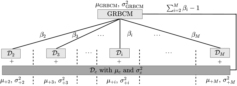
Figure 1: The GRBCM aggregation model.

In (14a) and (14b), the parameter $\beta_{i}$ ($i>2$) akin to that of RBCM is defined as the difference in the differential entropy between the base predictive distribution $p_{c}(y_{*}|\mathcal{D}_{c},\bm{x}_{*})$ and the enhanced predictive distribution $p_{+i}(y_{*}|\mathcal{D}_{+i},\bm{x}_{*})$ as

$$\beta_{i}=\left\{\begin{aligned} &1,&i=2,\\ &0.5(\log\sigma_{c}^{2}(\bm{x}_{*})-\log\sigma_{+i}^{2}(\bm{x}_{*})),&3\leq i\leq M.\end{aligned}\right.$$ (15)

It is found that after adding a subset $\mathcal{D}_{i}$ ($i\geq 2$) into the communication subset $\mathcal{D}_{c}$, if there is little improvement of $p_{+i}(y_{*}|\mathcal{D}_{+i},\bm{x}_{*})$ over $p_{c}(y_{*}|\mathcal{D}_{c},\bm{x}_{*})$, we weak the vote of $\mathcal{M}_{+i}$ by assigning a small $\beta_{i}$ that approaches zero.

As for the size of $\bm{X}_{c}$, more data points bring more informative $\mathcal{M}_{c}$ and better GRBCM predictions at the cost of higher computing complexity. In this article, we assign all the experts with the same training size as $n_{c}=n_{i}=m_{0}$ and $n_{+i}=2m_{0}$ for $2\leq i\leq M$.

Next, we show that the GRBCM’s predictive distribution will converge to the underlying true predictive distribution when $n\to\infty$.

Proposition 3.

Let $\{\mathcal{D}_{i}\}_{i=1}^{M_{n}}$ be a partition of the training data $\mathcal{D}$ with (i) $\lim_{n\to\infty}M_{n}=\infty$ and (ii) $\lim_{n\to\infty}n/M_{n}^{2}>0$. Besides, among the $M$ subsets, there is a global communication subset $\mathcal{D}_{c}$, the points in which are randomly selected from $\mathcal{D}$ without replacement. Let the global expert $\mathcal{M}_{c}$ and the enhanced experts $\{\mathcal{M}_{+i}\}_{i=2}^{M_{n}}$ be GPs with zero mean and stationary covariance function $k(.)>0$. Then, GRBCM yields consistent predictions as

$$\left\{\begin{aligned} \lim_{n\to\infty}\mu_{\mathrm{GRBCM}}(\bm{x}_{*})&=\mu_{\eta}(\bm{x}_{*}),\\ \lim_{n\to\infty}\sigma^{2}_{\mathrm{GRBCM}}(\bm{x}_{*})&=\sigma^{2}_{\eta}.\end{aligned}\right.$$ (16)

The detailed proof is provided in Appendix C. It is found in Proposition 3 that apart from the requirement that the communication subset $\mathcal{D}_{c}$ should be a random subset, the consistency of GRBCM holds for any partition of the remaining data $\mathcal{D}\backslash\mathcal{D}_{c}$. Besides, according to Propositions 2 and 3, both GPoE and GRBCM produce consistent predictions using random partition. It is known that the GP model $\mathcal{M}$ provides more confident predictions, i.e., lower uncertainty $U(\mathcal{M})=\int\sigma^{2}({\bm{x}})d\bm{x}$, with more data points. Since GRBCM trains experts on more informative subsets $\{\mathcal{D}_{+i}\}_{i=2}^{M}$, we have the following finding.

Remark 3.

When using random subsets, the GRBCM’s prediction uncertainty is always lower than that of GPoE, since the discrepancy $\delta_{U^{-1}}=U_{\mathrm{GRBCM}}^{-1}-U_{\mathrm{GPoE}}^{-1}$ satisfies

$$\delta_{U^{-1}}= \left[U^{-1}(\mathcal{M}_{+2})-\frac{1}{M_{n}}\sum_{i=1}^{M_{n}}U^{-1}(\mathcal{M}_{i})\right]$$

$$+ \int\sum_{i=3}^{M_{n}}\beta_{i}\left(\sigma_{+i}^{-2}(\bm{x}_{*})-\sigma_{c}^{-2}(\bm{x}_{*})\right)d\bm{x}_{*}>0$$

for a large enough $n$. It means compared to GPoE, GRBCM converges faster to the underlying function when $n\to\infty$.

Finally, similar to RBCM, GRBCM can be executed in multi-layer computing architectures with identical predictions (Deisenroth & Ng, 2015; Ionescu, 2015), which allow to run optimally and efficiently with the available computing infrastructure for distributed computing.

3.2 Complexity

Assuming that the experts $\{\mathcal{M}_{i}\}_{i=1}^{M}$ have the same training size $n_{i}=m_{0}=n/M$ for $1\leq i\leq M$. Compared to (G)PoE and (R)BCM, the proposed GRBCM has a higher time complexity in prediction due to the construction of new experts $\{\mathcal{M}_{+i}\}_{i=2}^{M}$. In prediction, it first needs to calculate the inverse of $k(\bm{X}_{c},\bm{X}_{c})$ and $M-1$ augmented covariance matrices $\{k(\{\bm{X}_{i},\bm{X}_{c}\},\{\bm{X}_{i},\bm{X}_{c}\})\}_{i=2}^{M}$, which scales as $\mathcal{O}(8nm_{0}^{2}-7m_{0}^{3})$, in order to obtain the predictions $\mu_{c}$, $\{\mu_{+i}\}_{i=2}^{M}$ and $\sigma^{2}_{c}$, $\{\sigma^{2}_{+i}\}_{i=2}^{M}$. Then, it combines the predictions of $\mathcal{M}_{c}$ and $\{\mathcal{M}_{+i}\}_{i=2}^{M}$ at $n^{\prime}$ test points. Therefore, the time complexity of the GRBCM prediction process is $\mathcal{O}(\alpha nm_{0}^{2})+\mathcal{{O}}(\beta n^{\prime}nm_{0})$, where $\alpha=(8M-7)/M$ and $\beta=(4M-3)/M$.

4 Numerical experiments

4.1 Toy example

We employ a 1D toy example

$$f(x) =5x^{2}\sin(12x)+(x^{3}-0.5)\sin(3x-0.5)$$ (17)

$$+4\cos(2x)+\epsilon,$$

where $\epsilon\sim\mathcal{N}(0,0.25)$, to illustrate the characteristics of existing aggregation models.

We generate $n=10^{4}$, $5\times 10^{4}$, $10^{5}$, $5\times 10^{5}$ and $10^{6}$ training points, respectively, in $[0,1]$, and select $n^{\prime}=0.1n$ test points randomly in $[-0.2,1.2]$. We pre-normalize each column of $\bm{X}$ and $\bm{y}$ to zero mean and unit variance. Due to the global expert $\mathcal{M}_{c}$ in GRBCM, we slightly modify the disjoint partition: we first generate a random subset and then use the k-means technique to generate $M-1$ disjoint subsets. Each expert is assigned with $m_{0}=500$ data points. We implement the aggregations by the GPML toolbox using the SE kernel in (1) and the conjugate gradients algorithm with the maximum number of evaluations as 500, and execute the code on a workstation with four 3.70 GHz cores and 16 GB RAM (multi-core computing in Matalb is employed). Finally, we use the Standardized Mean Square Error (SMSE) to evaluate the accuracy of prediction mean, and the Mean Standardized Log Loss (MSLL) to quantify the quality of predictive distribution (Rasmussen & Williams, 2006).

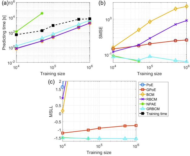
Figure 2: Comparison of different aggregation models on the toy example in terms of (a) computing time, (b) SMSE and (c) MSLL.

Fig. 2 depicts the comparative results of six aggregation models on the toy example. Note that NPAE using $n>5\times 10^{4}$ is unavailable due to the time-consuming prediction process. Fig. 2(a) shows that these models require the same training time, but they differ in the predicting time. Due to the communication expert, the GRBCM’s predicting time slightly offsets the curves of (G)PoE and (R)BCM. The NPAE however exhibits significantly larger predicting time with increasing $M$ and $n^{\prime}$. Besides, Fig. 2(b) and (c) reveal that GRBCM and NPAE yield better predictions with increasing $n$, which confirm their consistency when $n\to\infty$. As for NPAE, though performing slightly better than GRBCM using $n=5\times 10^{4}$, it requires several orders of magnitude larger predicting time, rendering it unsuitable for cases with many test points and subsets.

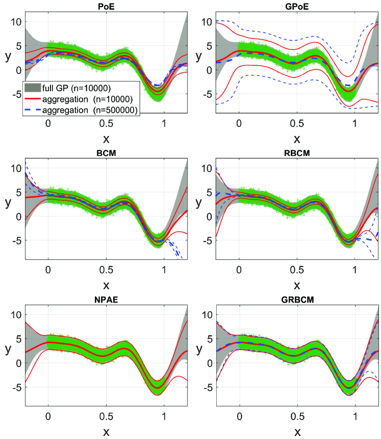
Figure 3: Illustrations of the aggregation models on the toy example. The green “+” symbols represent the $10^{4}$ data points. The shaded area indicates 99% confidence intervals of the full GP predictions using $n=10^{4}$.

Fig. 3 illustrates the six aggregation models using $n=10^{4}$ and $n=5\times 10^{5}$, respectively, in comparison to the full GP (ground truth) using $n=10^{4}$. It is observed that in terms of prediction mean, as discussed in remark 1, PoE and GPoE provide poorer results in the entire domain with increasing $n$. On the contrary, BCM and RBCM provide good predictions in the range $[0,1]$. As discussed in remark 2, BCM however yields unreliable predictions when leaving the training data. RBCM alleviates the issue by using a varying $\beta_{i}$. In terms of prediction variance, with increasing $n$, PoE and (R)BCM tend to shrink to zero (overconfident), while GPoE tends to approach $\sigma^{2}_{**}$ (too conservative). Particularly, PoE always has the largest MSLL value in Fig. 2(b), since as discussed in remark 2, its prediction variance approaches zero faster.

4.2 Medium-scale datasets

We use two realistic datasets, kin40k (8D, $10^{4}$ training points, $3\times 10^{4}$ test points) (Seeger et al., 2003) and sarcos (21D, 44484 training points, 4449 test points) (Rasmussen & Williams, 2006), to assess the performance of our approach.

The comparison includes all the aggregations except the expensive NPAE. Besides, we employ the fully independent training conditional (FITC) (Snelson & Ghahramani, 2006), the GP using stochastic variational inference (SVI) (Hensman et al., 2013), and the subset-of-data (SOD) (Chalupka et al., 2013) for comparison. We select the inducing size $m$ for FITC and SVI, the batch size $m_{b}$ for SVI, and the subset size $m_{\mathrm{sod}}$ for SOD, such that the computing time is similar to or a bit larger than that of GRBCM. Particularly, we choose $m=200$, $m_{b}=0.1n$ and $m_{\mathrm{sod}}=2500$ for kin40k, and $m=300$, $m_{b}=0.1n$ and $m_{\mathrm{sod}}=3000$ for sarcos. Differently, SVI employs the stochastic gradients algorithm with $t_{\mathrm{sg}}=1200$ iterations. Finally, we adopt the disjoint partition used before to divide the kin40k dataset into 16 subsets, and the sarcos dataset into 72 subsets for the aggregations. Each experiment is repeated ten times.

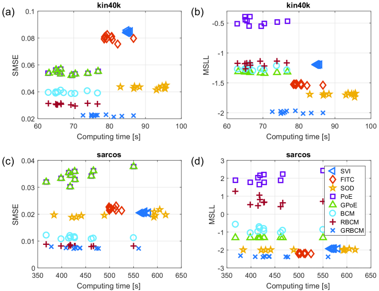
Figure 4: Comparison of the approximation models on the kin40k and sarcos datasets.

Fig. 4 depicts the comparative results of different approximation models over 10 runs on the kin40k and sarcos datasets. The horizontal axis represents the sum of training and predicting time. It is first observed that GRBCM provides the best performance on the two datasets in terms of both SMSE and MSLL at the cost of requiring a bit more computing time than (G)PoE and (R)BCM. As for (R)BCM, the small SMSE values reveal that they provide better prediction mean than FITC and SOD; but the large MSLL values again confirm that they provide overconfident prediction variance. As for (G)PoE, they suffer from poor prediction mean, as indicated by the large SMSE; but GPoE performs well in terms of MSLL. Finally, the simple SOD outperforms FITC and SVI on the kin40k dataset, and performs similarly on the sarcos dataset, which are consistent with the findings in (Chalupka et al., 2013).

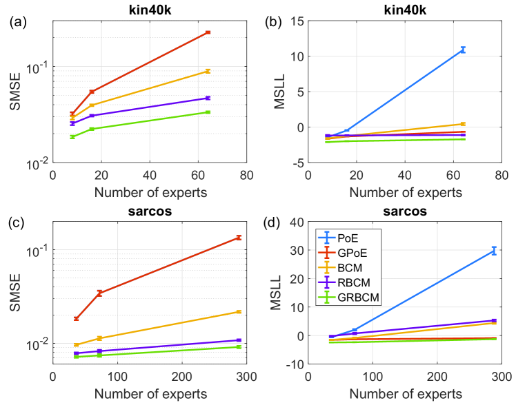
Figure 5: Comparison of the aggregation models using different numbers of experts on the kin40k and sarcos datasets.

Next, we explore the impact of the number $M$ of experts on the performance of aggregations. To this end, we run them on the kin40k dataset with $M$ respectively being 8, 16 and 64, and we run on the sarcos dataset with $M$ respectively being 36, 72 and 288. The results in Fig. 5 turn out that all the aggregations perform worse with increasing $M$, since the experts become weaker; but GRBCM still yields the best performance with different $M$. Besides, with increasing $M$, the poor prediction mean and the vanishing prediction variance of PoE result in the sharp increase of MSLL values.

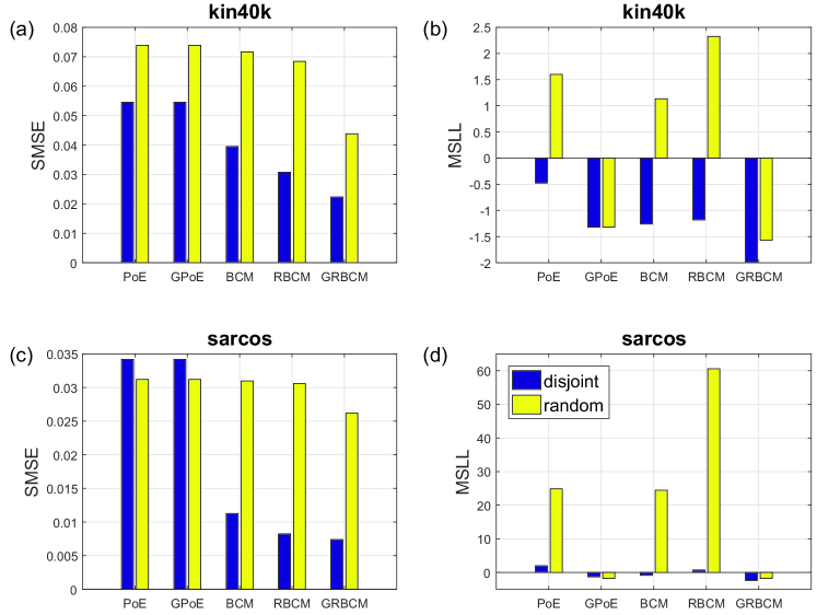
Figure 6: Comparison of the aggregation models using disjoint and random partitions on the kin40k dataset ($M=16$) and the sarcos dataset ($M=72$).

Finally, we investigate the impact of data partition (disjoint or random) on the performance of aggregations. The average results in Fig. 6 turn out that the disjoint partition is more beneficial for the aggregations. The results are expectable since the disjoint subsets provide separate and refined local information, whereas the random subsets provide overlapping and coarse global information. But we observe that GPoE performs well on the sarcos dataset using random partition, which confirms the conclusions in Proposition 2. Besides, as revealed in remark 3, even using random partition, GRBCM outperforms GPoE.

4.3 Large-scale datasets

This section explores the performance of aggregations and SVI on two large-scale datasets. We first assess them on the 90D song dataset, which is a subset of the million song dataset (Bertin-Mahieux et al., 2011). The song dataset is partitioned into 450000 training points and 65345 test points. We then assess the models on the 11D electric dataset that is partitioned into 1.8 million training points and 249280 test points. We follow the normalization and data pre-processing in (Wilson et al., 2016) to generate the two datasets. For the song dataset, we use the foregoing disjoint partition to divide it into $M=720$ subsets, and use $m=800$, $m_{b}=5000$ and $t_{\mathrm{sg}}=1300$ for SVI; for the electric dataset, we divide it into $M=2880$ subsets, and use $m=1000$, $m_{b}=5000$ and $t_{\mathrm{sg}}=1500$ for SVI. As a result, each expert is assigned with $m_{0}=625$ data points for the aggregations.

Table 1: Comparative results of the aggregation models and SVI on the song and electric datasets.

	song (450K)		electric (1.8M)
	SMSE	MSLL	SMSE	MSLL
PoE	0.8527	328.82	0.1632	1040.3
GPoE	0.8527	0.1159	0.1632	24.940
BCM	2.6919	156.62	0.0073	51.081
RBCM	1.3383	24.930	0.0027	85.657
SVI	0.7909	-0.1885	0.0042	-1.1410
GRBCM	0.7321	-0.1571	0.0024	-1.3161

Table 1 reveals that the (G)PoE’s SMSE value is smaller than that of (R)BCM on the song dataset. The poor prediction mean of BCM is caused by the fact that the song dataset is highly clustered such that BCM suffers from weak experts in regions with scarce points. On the contrary, due to the almost uniform distribution of the electric data points, the (R)BCM’s SMSE is much smaller than that of (G)PoE. Besides, unlike the vanishing prediction variances of PoE and (R)BCM when $n\to\infty$, GPoE provides conservative prediction variance, resulting in small MSLL values on the two datasets. The proposed GRBCM always outperforms the other aggregations in terms of both SMSE and MSLL on the two datasets due to the consistency. Finally, GRBCM performs similarly to SVI on the song dataset; but GRBCM outperforms SVI on the electric dataset.

5 Conclusions

To scale the standard GP to large-scale regression, we present the GRBCM aggregation model, which introduces a global communication expert to yield consistent yet efficient predictions when $n\to\infty$. Through theoretical and empirical analyses, we demonstrated the superiority of GRBCM over existing aggregations on datasets with up to 1.8M training points.

The superiority of local experts is the capability of capturing local patterns. Hence, further works will consider the experts with individual hyperparameters in order to capture non-stationary and heteroscedastic features.

Appendix A Proof of Proposition 1

With disjoint partition, we consider two extreme local GP experts. For the first extreme expert $\mathcal{M}_{a_{n}}$ ($1\leq a_{n}\leq M_{n}$), the test point $\bm{x}_{*}$ falls into the local region defined by $\bm{X}_{a_{n}}$, i.e., $\bm{x}_{*}$ is adherent to $\bm{X}_{a_{n}}$ when $n\to\infty$. Hence, we have (Vazquez & Bect, 2010)

$$\lim_{n\to\infty}\sigma^{2}_{a_{n}}(\bm{x}_{*})=\lim_{n\to\infty}\sigma^{2}_{\epsilon,n}=\sigma^{2}_{\eta}.$$

For the other extreme expert $\mathcal{M}_{b_{n}}$, it lies farthest away from $\bm{x}_{*}$ such that the related prediction variance $\sigma^{2}_{b_{n}}(\bm{x}_{*})$ is closest to $\sigma^{2}_{**}$. It is known that for any $\mathcal{M}_{i}$ ($i\neq a_{n}$) where $\bm{x}_{*}$ is away from the training data $\bm{X}_{i}$, given the relative distance $r_{i}=\min\|\bm{x}_{*}-\bm{x}\|_{\forall\bm{x}\in\bm{X}_{i}}$, we have $\lim_{r_{i}\to\infty}\sigma^{2}_{i}(\bm{x}_{*})=\sigma^{2}_{**}$. Since, however, we here focus on the GP predictions in the bounded region $\Omega\in[0,1]^{d}$ and employ the covariance function $k(.)>0$, then the positive sequence $c_{n}=\{\sigma^{-2}_{b_{n}}(\bm{x}_{*})-\sigma^{-2}_{**}\}$ is small but satisfies $\lim_{n\to\infty}c_{n}>0$ and

$$\sigma^{-2}_{i}(\bm{x}_{*})-\sigma^{-2}_{**}\geq c_{n},\,1\leq i\neq a_{n}\leq M_{n}.$$

The equality holds only when $i=b_{n}$.

Thereafter, with the sequence $\epsilon_{n}=\min\{c_{n},\frac{1}{M_{n}^{\alpha}}\}\to_{n\to\infty}0$ where $\alpha>0$ we have

$$\sigma^{-2}_{i}(\bm{x}_{*})-\sigma^{-2}_{**}\geq c_{n}\geq\epsilon_{n},\,1\leq i\neq a_{n}\leq M_{n}.$$

It is found that $c_{n}=\epsilon_{n}$ is possible to hold only when $M_{n}$ is small. With the increase of $n$, $\epsilon_{n}$ quickly becomes much smaller than $c_{n}$ since $\lim_{n\to\infty}1/M_{n}^{\alpha}=0$.

The typical aggregated prediction variance writes

$$\sigma^{-2}_{\mathcal{A},n}(\bm{x}_{*}) =\sum_{i=1}^{M_{n}}\beta_{i}(\sigma^{-2}_{i}(\bm{x}_{*})-\sigma^{-2}_{**})+\sigma^{-2}_{**},$$ (18)

where for (G)PoE we remove the prior precision $\sigma^{-2}_{**}$. We prove below the inconsistency of (G)PoE and (R)BCM using disjoint partition.

For PoE, (18) is $\sum_{i=1}^{M_{n}}\sigma_{i}^{-2}(\bm{x}_{*})>M_{n}\sigma^{-2}_{**}\to_{n\to\infty}\infty$, leading to the inconsistent variance $\lim_{n\to\infty}\sigma^{2}_{\mathcal{A},n}=0$. For (R)BCM, the first term of $\sigma^{-2}_{\mathcal{A},n}(\bm{x}_{*})$ in (18) satisfies, given that $n$ is large enough,

$$\sum_{i=1}^{M_{n}}\beta_{i}(\sigma^{-2}_{i}(\bm{x}_{*})-\sigma^{-2}_{**})>\epsilon_{n}\sum_{i=1}^{M_{n}}\beta_{i}=\frac{1}{M_{n}^{\alpha}}\sum_{i=1}^{M_{n}}\beta_{i}.$$

Taking $\beta_{i}=1$ for BCM and $\alpha=0.5$, we have $\frac{1}{M_{n}^{\alpha}}\sum_{i=1}^{M_{n}}\beta_{i}=\sqrt{M_{n}}\to_{n\to\infty}\infty$, leading to the inconsistent variance $\lim_{n\to\infty}\sigma^{2}_{\mathcal{A},n}=0$. For RBCM, since

$$\beta_{i}=0.5(\log\sigma_{**}^{2}-\log\sigma_{i}^{2}(\bm{x}_{*}))\geq 0.5\log(1+c_{n}\sigma^{2}_{**})$$

where the equality holds only when $i=b_{n}$, we have $\frac{1}{M_{n}^{\alpha}}\sum_{i=1}^{M_{n}}\beta_{i}>0.5\log(1+c_{n}\sigma^{2}_{**})\sqrt{M_{n}}\to_{n\to\infty}\infty$, leading to the inconsistent variance $\lim_{n\to\infty}\sigma^{2}_{\mathcal{A},n}=0$.

Finally, for GPoE, we know that when $n\to\infty$, $\sigma^{-2}_{a_{n}}(\bm{x}_{*})$ converges to $\sigma^{-2}_{\eta}$; but the other prediction precisions satisfy $c_{n}+\sigma^{-2}_{**}\leq\sigma^{-2}_{i}(\bm{x}_{*})<\sigma^{-2}_{\epsilon,n}\to_{n\to\infty}\sigma_{\eta}^{-2}$ for $1\leq i\neq a_{n}\leq M_{n}$, since $\bm{x}_{*}$ is away from their training points. Hence, we have

$$\lim_{n\to\infty}\left(\sigma^{-2}_{\eta}-\sigma^{-2}_{\mathrm{GPoE}}(\bm{x}_{*})\right)$$

$$= \lim_{n\to\infty}\frac{1}{M_{n}}\left(\sigma^{-2}_{\eta}-\sigma^{-2}_{a_{n}}(\bm{x}_{*})\right)$$

$$+\lim_{n\to\infty}\frac{1}{M_{n}}\sum_{i\neq a_{n}}^{M_{n}}\left(\sigma^{-2}_{\eta}-\sigma^{-2}_{i}(\bm{x}_{*})\right)$$

$$> \lim_{n\to\infty}\frac{1}{M_{n}}\left(\sigma^{-2}_{\eta}-\sigma^{-2}_{a_{n}}(\bm{x}_{*})\right)$$

$$+\lim_{n\to\infty}\frac{1}{M_{n}}\sum_{i\neq a_{n}}^{M_{n}}\left(\sigma^{-2}_{\eta}-\sigma^{-2}_{\epsilon,n}(\bm{x}_{*})\right)=0,$$

which means that $\sigma^{2}_{\mathrm{GPoE}}(\bm{x}_{*})$ is inconsistent since $\lim_{n\to\infty}\sigma^{2}_{\mathrm{GPoE}}(\bm{x}_{*})>\sigma^{2}_{\eta}$. Meanwhile, we easily find that $\lim_{n\to\infty}\sigma^{-2}_{\mathrm{GPoE}}(\bm{x}_{*})>c_{n}+\sigma^{-2}_{**}$, leading to $\lim_{n\to\infty}\sigma^{2}_{\mathrm{GPoE}}(\bm{x}_{*})<\sigma^{2}_{b_{n}}(\bm{x}_{*})<\sigma^{2}_{**}$.

Appendix B Proof of Proposition 2

With smoothness assumption and particularly distributed noise (normal or Laplacian distribution), it has been proved that the GP predictions would converge to the true predictions when $n\to\infty$ (Choi & Schervish, 2004). Hence, given that the points in $\bm{X}_{i}$ are randomly selected without replacement from $\bm{X}$ and $n_{i}=n/M_{n}\to_{n\to\infty}\infty$, we have

$$\lim_{n\to\infty}\mu_{i}(\bm{x}_{*})=\mu_{\eta}(\bm{x}_{*}),\lim_{n\to\infty}\sigma^{2}_{i}(\bm{x}_{*})=\sigma^{2}_{\eta},\quad 1\leq i\leq M_{n}.$$

For the aggregated prediction variance, we have

$$\lim_{n\to\infty}\sigma_{\mathcal{A},n}^{-2}(\bm{x}_{*})=\lim_{n\to\infty}\left[\sum_{i=1}^{M_{n}}\beta_{i}(\sigma_{i}^{-2}(\bm{x}_{*})-\sigma_{**}^{-2})+\sigma_{**}^{-2}\right],$$

where for (G)PoE we remove $\sigma^{-2}_{**}$. For PoE, given $\beta_{i}=1$ and $\lim_{n\to\infty}\sigma^{-2}_{i}(\bm{x}_{*})=\sigma^{-2}_{\eta}$, we have the inconsistent variance $\lim_{n\to\infty}\sigma_{\mathcal{A},n}^{-2}(\bm{x}_{*})=\lim_{n\to\infty}M_{n}\sigma_{\eta}^{-2}=\infty$. For GPoE, given $\beta_{i}=1/M_{n}$ we have the consistent variance $\lim_{n\to\infty}\sigma_{\mathcal{A},n}^{-2}(\bm{x}_{*})=M_{n}\frac{1}{M_{n}}\sigma_{\eta}^{-2}=\sigma_{\eta}^{-2}$. For BCM, given $\beta_{i}=1$ we have the inconsistent variance $\lim_{n\to\infty}\sigma_{\mathcal{A},n}^{-2}(\bm{x}_{*})=\lim_{n\to\infty}[M_{n}(\sigma_{\eta}^{-2}-\sigma_{**}^{-2})+\sigma_{**}^{-2}]=\infty$. Finally, for RBCM, given $\lim_{n\to\infty}\beta_{i}=\overline{\beta}=0.5\log(\sigma^{2}_{**}/\sigma^{2}_{\eta})$, we have the inconsistent variance $\lim_{n\to\infty}\sigma_{\mathcal{A},n}^{-2}(\bm{x}_{*})=\lim_{n\to\infty}[M_{n}\overline{\beta}(\sigma_{\eta}^{-2}-\sigma_{**}^{-2})+\sigma_{**}^{-2}]=\infty$.

Then, for the aggregated prediction mean we have

$$\lim_{n\to\infty}\mu_{\mathcal{A},n}(\bm{x}_{*})=\lim_{n\to\infty}\sigma_{\mathcal{A},n}^{2}(\bm{x}_{*})\sum_{i=1}^{M_{n}}\beta_{i}\sigma^{-2}_{i}(\bm{x}_{*})\mu_{i}(\bm{x}_{*}).$$

For PoE, given $\beta_{i}=1$ and $\lim_{n\to\infty}\sigma^{-2}_{i}(\bm{x}_{*})/\sigma_{\mathcal{A},n}^{-2}(\bm{x}_{*})=1/M_{n}$, we have the consistent prediction mean $\lim_{n\to\infty}\mu_{\mathcal{A},n}(\bm{x}_{*})=\mu_{\eta}(\bm{x}_{*})$. For GPoE, given $\beta_{i}=1/M_{n}$ and $\lim_{n\to\infty}\sigma^{-2}_{i}(\bm{x}_{*})/\sigma_{\mathcal{A},n}^{-2}(\bm{x}_{*})=1$, we have the consistent prediction mean $\lim_{n\to\infty}\mu_{\mathcal{A},n}(\bm{x}_{*})=\mu_{\eta}(\bm{x}_{*})$. For (R)BCM, given $\beta_{i}=\overline{\beta}=1$ or $\lim_{n\to\infty}\beta_{i}=\overline{\beta}=0.5\log(\sigma^{2}_{**}/\sigma^{2}_{\eta})$, we have the inconsistent prediction mean $\lim_{n\to\infty}\mu_{\mathcal{A},n}(\bm{x}_{*})=\lim_{n\to\infty}\overline{\beta}\sigma^{-2}_{\eta}\mu_{\eta}(\bm{x}_{*})/(\overline{\beta}(\sigma^{-2}_{\eta}-\sigma^{-2}_{**})+\sigma^{-2}_{**}/M_{n})=a\mu_{\eta}(\bm{x}_{*})$ where $a=\sigma_{\eta}^{-2}/(\sigma_{\eta}^{-2}-\sigma_{**}^{-2})\geq 1$ and the equality holds when $\sigma^{2}_{\eta}=0$.

Appendix C Proof of Proposition 3

Given that the points in the communication subset $\mathcal{D}_{c}$ are randomly selected without replacement from $\mathcal{D}$ and $n_{c}=n/M_{n}\to_{n\to\infty}\infty$, we have $\lim_{n\to\infty}\mu_{c}(\bm{x}_{*})=\mu_{\eta}(\bm{x}_{*})$ and $\lim_{n\to\infty}\sigma^{2}_{c}(\bm{x}_{*})=\sigma^{2}_{\eta}$ for $\mathcal{M}_{c}$. Likewise, for the expert $\mathcal{M}_{+i}$ trained on the augmented dataset $\mathcal{D}_{+i}=\{\mathcal{D}_{i},\mathcal{D}_{c}\}$ with size $n_{+i}=2n/M_{n}$, we have $\lim_{n\to\infty}\mu_{+i}(\bm{x}_{*})=\mu_{\eta}(\bm{x}_{*})$ and $\lim_{n\to\infty}\sigma^{2}_{+i}(\bm{x}_{*})=\sigma^{2}_{\eta}$ for $2\leq i\leq M$.

We first derive the upper bound of $\sigma^{2}_{c}(\bm{x}_{*})$. For the stationary covariance function $k(.)>0$, when $n_{c}$ is large enough we have (Vazquez & Bect, 2010)

$$\sigma^{2}_{c}(\bm{x}_{*})\leq k(\bm{x}_{*},\bm{x}_{*})-\frac{k^{2}(\bm{x}_{*},\bm{x}^{\prime})}{k(\bm{x}^{\prime},\bm{x}^{\prime})}+\sigma^{2}_{\epsilon,n},$$

where $\bm{x}^{\prime}\in\bm{X}_{c}$ is the nearest data point to $\bm{x}_{*}$. It is known that the relative distance $r_{c}=\|\bm{x}_{*}-\bm{x}^{\prime}\|$ is proportional to the inverse of the training size $n_{c}$, i.e., $r_{c}\propto 1/n_{c}=M_{n}/n\to_{n\to\infty}0$. Conventional stationary covariance functions only relay on the relative distance (once the covariance parameters have been determined) and decrease with $r_{c}$. Consequently, the prediction variance $\sigma^{2}_{c}(\bm{x}_{*})$ increases with $r_{c}$. Taking the SE covariance function in (1) for example, when $r_{c}\to 0$ we have, given $l_{0}=\min_{1\leq i\leq d}\{l_{i}\}$,

$$\sigma^{2}_{c}(\bm{x}_{*}) \leq\sigma^{2}_{f}-\sigma^{2}_{f}\exp(-r_{c}^{2}/l_{0}^{2})+\sigma^{2}_{\epsilon,n}$$ (19)

$$<\frac{\sigma^{2}_{f}}{l_{0}^{2}}r_{c}^{2}+\sigma^{2}_{\epsilon,n}=ar_{c}^{2}+\sigma^{2}_{\epsilon,n}.$$

We clearly see from this inequality that when $r_{c}\to 0$, $\sigma^{2}_{c}(\bm{x}_{*})$ goes to $\sigma^{2}_{\eta}$ since $\lim_{n\to\infty}\sigma^{2}_{\epsilon,n}=\sigma^{2}_{\eta}$.

Then, we rewrite the precision of GRBCM in (14b) as, given $\beta_{2}=1$,

$$\sigma_{\mathrm{GRBCM}}^{-2}(\bm{x}_{*})=\sigma_{+2}^{-2}(\bm{x}_{*})+\sum_{i=3}^{M_{n}}\beta_{i}\left(\sigma_{+i}^{-2}(\bm{x}_{*})-\sigma_{c}^{-2}(\bm{x}_{*})\right).$$ (20)

Compared to $\mathcal{M}_{c}$, $\mathcal{M}_{+i}$ is trained on a more dense dataset $\mathcal{D}_{+i}$, leading to $\sigma^{2}_{+i}(\bm{x}_{*})\leq\sigma^{2}_{c}(\bm{x}_{*})$ for a large enough $n$.

Given (19) and $\sigma^{2}_{+i}(\bm{x}_{*})>\sigma^{2}_{\epsilon,n}$, the weight $\beta_{i}$ satisfies, for $3\leq i\leq M_{n}$,

$$0\leq\beta_{i} =\frac{1}{2}\log\left(\frac{\sigma_{c}^{2}(\bm{x}_{*})}{\sigma_{+i}^{2}(\bm{x}_{*})}\right)<\frac{1}{2}\log\left(\frac{\sigma_{c}^{2}(\bm{x}_{*})}{\sigma^{2}_{\epsilon,n}}\right)$$ (21)

$$<\frac{1}{2}\log\left(\frac{ar_{c}^{2}+\sigma^{2}_{\epsilon,n}}{\sigma^{2}_{\epsilon,n}}\right)\leq\frac{a}{2\sigma^{2}_{\epsilon,n}}r_{c}^{2}.$$

Besides, the precision discrepancy satisfies, for $3\leq i\leq M_{n}$,

$$0\leq\sigma_{+i}^{-2}(\bm{x}_{*})-\sigma_{c}^{-2}(\bm{x}_{*}) =\sigma_{c}^{-2}(\bm{x}_{*})\left(\frac{\sigma_{c}^{2}(\bm{x}_{*})}{\sigma_{+i}^{2}(\bm{x}_{*})}-1\right)$$ (22)

$$<\frac{1}{\sigma^{2}_{\epsilon,n}}\frac{a}{\sigma^{2}_{\epsilon,n}}r_{c}^{2}.$$

Hence, the second term in the right-hand side of (20) satisfies

$$\sum_{i=3}^{M_{n}}\beta_{i}\left(\sigma_{+i}^{-2}(\bm{x}_{*})-\sigma_{c}^{-2}(\bm{x}_{*})\right)<\sum_{i=3}^{M_{n}}\frac{a^{2}}{2\sigma^{6}_{\epsilon,n}}r_{c}^{4}\propto\frac{M_{n}^{5}}{n^{4}}.$$

Since $\lim_{n\to\infty}n/M_{n}^{2}>0$, we have $\lim_{n\to\infty}n^{4}/M_{n}^{5}=\infty$, and furthermore,

$$\lim_{n\to\infty}\sum_{i=3}^{M_{n}}\beta_{i}\left(\sigma_{+i}^{-2}(\bm{x}_{*})-\sigma_{c}^{-2}(\bm{x}_{*})\right)=0.$$ (23)

Substituting (23) and $\lim_{n\to\infty}\sigma_{+2}^{-2}(\bm{x}_{*})=\sigma^{-2}_{\eta}$ into (20), we have a consistent prediction precision as

$$\lim_{n\to\infty}\sigma_{\mathrm{GRBCM}}^{-2}(\bm{x}_{*})=\sigma^{-2}_{\eta}.$$

Similarly, we rewrite the GRBCM’s prediction mean in (14a) as

$$\mu_{\mathrm{GRBCM}}(\bm{x}_{*})=\sigma_{\mathrm{GRBCM}}^{2}(\bm{x}_{*})\left(\mu_{\Delta}+\sigma_{+2}^{-2}(\bm{x}_{*})\mu_{+2}(\bm{x}_{*})\right),$$ (24)

where

$$\mu_{\Delta}=\sum_{i=3}^{M_{n}}\beta_{i}\left(\sigma_{+i}^{-2}(\bm{x}_{*})\mu_{+i}(\bm{x}_{*})-\sigma_{c}^{-2}(\bm{x}_{*})\mu_{c}(\bm{x}_{*})\right).$$

Let $\delta_{\mathrm{max}}=\max_{3\leq i\leq M_{n}}\left|\frac{\sigma_{c}^{2}(\bm{x}_{*})}{\sigma_{+i}^{2}(\bm{x}_{*})}\mu_{+i}(\bm{x}_{*})-\mu_{c}(\bm{x}_{*})\right|\to_{n\to\infty}0$, we have

$$\left|\mu_{\Delta}\right| \leq\sum_{i=3}^{M_{n}}\beta_{i}\sigma_{c}^{-2}\left|\frac{\sigma_{c}^{2}(\bm{x}_{*})}{\sigma_{+i}^{2}(\bm{x}_{*})}\mu_{+i}(\bm{x}_{*})-\mu_{c}(\bm{x}_{*})\right|$$ (25)

$$\mathop{<}^{\mathrm{Eq.}\eqref{Eq_beta_i_UB}}\sum_{i=3}^{M_{n}}\frac{ar_{c}^{2}}{2\sigma^{4}_{\epsilon,n}}\delta_{\mathrm{max}}\to_{n\to\infty}0.$$

Substituting (25) into (24), we have the consistent prediction mean as

$$\lim_{n\to\infty}\mu_{\mathrm{GRBCM}}(\bm{x}_{*})=\mu_{\eta}(\bm{x}_{*}).$$

Appendix D Discussions of GRBCM on the toy example

It is observed that the proposed GRBCM showcases superiority over existing aggregations on the toy example, which is brought by the particularly designed aggregation structure: the global communication expert $\mathcal{M}_{c}$ to capture the long-term features of the target function, and the remaining experts $\{\mathcal{M}_{+i}\}_{i=2}^{M}$ to refine local predictions.

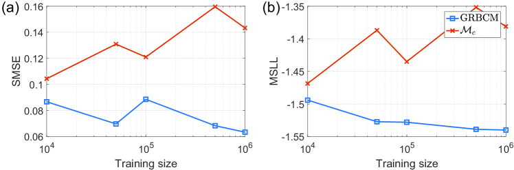
Figure 7: Comparative results of GRBCM and $\mathcal{M}_{c}$ on the toy example.

To verify the capability of GRBCM, we compare it with the pure global expert $\mathcal{M}_{c}$ which relies on a random subset $\bm{X}_{c}$. Fig. 7 shows the comparative results of GRBCM and $\mathcal{M}_{c}$ on the toy example. It is found that with increasing $n$, (i) GRBCM always outperforms $\mathcal{M}_{c}$ because of the benefits brought by local experts; and (ii) the predictions of $\mathcal{M}_{c}$ generally become poorer since it becomes intractable to choose a good subset from the increasing dataset.

Appendix E Experimental results of NPAE

Table 2 compares the results of GRBCM and NPAE over 10 runs on the kin40k dataset ($M=16$) and the sarcos dataset ($M=72$) using disjoint partition. It is observed that GRBCM performs slightly better than NPAE on the kin40k dataset, and produces competitive results on the sarcos dataset. But in terms of the computing efficiency, since NPAE needs to build and invert an $M\times M$ covariance matrix at each test point, it requires much more running time, especially for the sarcos dataset with $M=72$.

Table 2: Comparative results (mean and standard deviation) of GRBCM and NPAE over 10 runs on the kin40k dataset ($M=16$) and the sarcos dataset ($M=72$) using disjoint partition. The computing time $t$ for each model involves the training and predicting time.

kin40k	GRBCM	NPAE
SMSE	0.0223 $\pm$ 0.0005	0.0246 $\pm$ 0.0007
MSLL	-1.9927 $\pm$ 0.0177	-1.9565 $\pm$ 0.0170
$t$ [s]	78.1 $\pm$ 4.4	2852.4 $\pm$ 16.7
sarcos	GRBCM	NPAE
SMSE	0.0074 $\pm$ 0.0002	0.0054 $\pm$ 0.0001
MSLL	-2.3681 $\pm$ 0.0242	-2.5900 $\pm$ 0.0068
$t$ [s]	445.6 $\pm$ 49.4	26444.0 $\pm$ 1213.0

References

- Alvarez et al. (2012) Alvarez, Mauricio A, Rosasco, Lorenzo, Lawrence, Neil D, et al. Kernels for vector-valued functions: A review. Foundations and Trends® in Machine Learning, 4(3):195–266, 2012.
- Bauer et al. (2016) Bauer, Matthias, van der Wilk, Mark, and Rasmussen, Carl Edward. Understanding probabilistic sparse Gaussian process approximations. In Advances in Neural Information Processing Systems, pp. 1533–1541. Curran Associates, Inc., 2016.
- Bertin-Mahieux et al. (2011) Bertin-Mahieux, Thierry, Ellis, Daniel PW, Whitman, Brian, and Lamere, Paul. The million song dataset. In ISMIR, pp. 1–6, 2011.
- Bui & Turner (2014) Bui, Thang D and Turner, Richard E. Tree-structured Gaussian process approximations. In Advances in Neural Information Processing Systems, pp. 2213–2221. Curran Associates, Inc., 2014.
- Cao & Fleet (2014) Cao, Yanshuai and Fleet, David J. Generalized product of experts for automatic and principled fusion of Gaussian process predictions. arXiv preprint arXiv:1410.7827, 2014.
- Chalupka et al. (2013) Chalupka, Krzysztof, Williams, Christopher KI, and Murray, Iain. A framework for evaluating approximation methods for Gaussian process regression. Journal of Machine Learning Research, 14(Feb):333–350, 2013.
- Choi & Schervish (2004) Choi, Taeryon and Schervish, Mark J. Posterior consistency in nonparametric regression problems under Gaussian process priors. Technical report, Carnegie Mellon University, 2004.
- Deisenroth & Ng (2015) Deisenroth, Marc Peter and Ng, Jun Wei. Distributed Gaussian processes. In International Conference on Machine Learning, pp. 1481–1490. PMLR, 2015.
- Fu et al. (2013) Fu, Yifan, Zhu, Xingquan, and Li, Bin. A survey on instance selection for active learning. Knowledge and Information Systems, 35(2):249–283, 2013.
- Gal et al. (2014) Gal, Yarin, van der Wilk, Mark, and Rasmussen, Carl Edward. Distributed variational inference in sparse Gaussian process regression and latent variable models. In Advances in Neural Information Processing Systems, pp. 3257–3265. Curran Associates, Inc., 2014.
- Genest & Zidek (1986) Genest, Christian and Zidek, James V. Combining probability distributions: A critique and an annotated bibliography. Statistical Science, 1(1):114–135, 1986.
- Hensman et al. (2013) Hensman, James, Fusi, Nicolò, and Lawrence, Neil D. Gaussian processes for big data. In Proceedings of the 29th Conference on Uncertainty in Artificial Intelligence, pp. 282–290. AUAI Press, 2013.
- Hinton (2002) Hinton, Geoffrey E. Training products of experts by minimizing contrastive divergence. Neural Computation, 14(8):1771–1800, 2002.
- Hoang et al. (2016) Hoang, Trong Nghia, Hoang, Quang Minh, and Low, Bryan Kian Hsiang. A distributed variational inference framework for unifying parallel sparse Gaussian process regression models. In International Conference on Machine Learning, pp. 382–391. PMLR, 2016.
- Ionescu (2015) Ionescu, Radu Cristian. Revisiting large scale distributed machine learning. arXiv preprint arXiv:1507.01461, 2015.
- Lawrence (2005) Lawrence, Neil. Probabilistic non-linear principal component analysis with Gaussian process latent variable models. Journal of Machine Learning Research, 6(Nov):1783–1816, 2005.
- Liu et al. (2017) Liu, Haitao, Cai, Jianfei, and Ong, Yew-Soon. An adaptive sampling approach for Kriging metamodeling by maximizing expected prediction error. Computers & Chemical Engineering, 106(Nov):171–182, 2017.
- Liu et al. (2018) Liu, Haitao, Cai, Jianfei, and Ong, Yew-Soon. Remarks on multi-output Gaussian process regression. Knowledge-Based Systems, 144(March):102–121, 2018.
- Moore & Russell (2015) Moore, David and Russell, Stuart J. Gaussian process random fields. In Advances in Neural Information Processing Systems, pp. 3357–3365. Curran Associates, Inc., 2015.
- Park et al. (2011) Park, Chiwoo, Huang, Jianhua Z, and Ding, Yu. Domain decomposition approach for fast Gaussian process regression of large spatial data sets. Journal of Machine Learning Research, 12(May):1697–1728, 2011.
- Peng et al. (2017) Peng, Hao, Zhe, Shandian, Zhang, Xiao, and Qi, Yuan. Asynchronous distributed variational Gaussian process for regression. In International Conference on Machine Learning, pp. 2788–2797. PMLR, 2017.
- Quiñonero-Candela & Rasmussen (2005) Quiñonero-Candela, Joaquin and Rasmussen, Carl Edward. A unifying view of sparse approximate Gaussian process regression. Journal of Machine Learning Research, 6(Dec):1939–1959, 2005.
- Ranjan & Gneiting (2010) Ranjan, Roopesh and Gneiting, Tilmann. Combining probability forecasts. Journal of the Royal Statistical Society: Series B (Statistical Methodology), 72(1):71–91, 2010.
- Rasmussen & Ghahramani (2002) Rasmussen, Carl E and Ghahramani, Zoubin. Infinite mixtures of Gaussian process experts. In Advances in Neural Information Processing Systems, pp. 881–888. Curran Associates, Inc., 2002.
- Rasmussen & Williams (2006) Rasmussen, Carl Edward and Williams, Christopher K. I. Gaussian processes for machine learning. MIT Press, 2006.
- Rullière et al. (2017) Rullière, Didier, Durrande, Nicolas, Bachoc, François, and Chevalier, Clément. Nested Kriging predictions for datasets with a large number of observations. Statistics and Computing, pp. 1–19, 2017.
- Seeger et al. (2003) Seeger, Matthias, Williams, Christopher, and Lawrence, Neil. Fast forward selection to speed up sparse Gaussian process regression. In Artificial Intelligence and Statistics, pp. EPFL–CONF–161318. PMLR, 2003.
- Shahriari et al. (2016) Shahriari, Bobak, Swersky, Kevin, Wang, Ziyu, Adams, Ryan P, and de Freitas, Nando. Taking the human out of the loop: A review of Bayesian optimization. Proceedings of the IEEE, 104(1):148–175, 2016.
- Snelson & Ghahramani (2006) Snelson, Edward and Ghahramani, Zoubin. Sparse Gaussian processes using pseudo-inputs. In Advances in Neural Information Processing Systems, pp. 1257–1264. MIT Press, 2006.
- Snelson & Ghahramani (2007) Snelson, Edward and Ghahramani, Zoubin. Local and global sparse Gaussian process approximations. In Artificial Intelligence and Statistics, pp. 524–531. PMLR, 2007.
- Tavassolipour et al. (2017) Tavassolipour, Mostafa, Motahari, Seyed Abolfazl, and Shalmani, Mohammad-Taghi Manzuri. Learning of Gaussian processes in distributed and communication limited systems. arXiv preprint arXiv:1705.02627, 2017.
- Titsias (2009) Titsias, Michalis K. Variational learning of inducing variables in sparse Gaussian processes. In Artificial Intelligence and Statistics, pp. 567–574. PMLR, 2009.
- Tresp (2000) Tresp, Volker. A Bayesian committee machine. Neural Computation, 12(11):2719–2741, 2000.
- Vazquez & Bect (2010) Vazquez, Emmanuel and Bect, Julien. Pointwise consistency of the Kriging predictor with known mean and covariance functions. In 9th International Workshop in Model-Oriented Design and Analysis, pp. 221–228. Springer, 2010.
- Wilson & Nickisch (2015) Wilson, Andrew and Nickisch, Hannes. Kernel interpolation for scalable structured Gaussian processes (KISS-GP). In International Conference on Machine Learning, pp. 1775–1784. PMLR, 2015.
- Wilson et al. (2016) Wilson, Andrew Gordon, Hu, Zhiting, Salakhutdinov, Ruslan, and Xing, Eric P. Deep kernel learning. In Artificial Intelligence and Statistics, pp. 370–378. PMLR, 2016.
- Yuan & Neubauer (2009) Yuan, Chao and Neubauer, Claus. Variational mixture of Gaussian process experts. In Advances in Neural Information Processing Systems, pp. 1897–1904. Curran Associates, Inc., 2009.