Dark side of the Seesaw

Abstract

In an attempt to unfold (if any) a possible connection between two apparently uncorrelated sectors, namely neutrino and dark matter, we consider the type-I seesaw and a fermion singlet dark matter to start with. Our construction suggests that there exists a scalar field mediator between these two sectors whose vacuum expectation value not only generates the mass of the dark matter, but also takes part in the neutrino mass generation. While the choice of $Z_{4}$ symmetry allows us to establish the framework, the vacuum expectation value of the mediator field breaks $Z_{4}$ to a remnant $Z_{2}$, that is responsible to keep dark matter stable. Therefore, the observed light neutrino masses and relic abundance constraint on the dark matter, allows us to predict the heavy seesaw scale as illustrated in this paper.The methodology to connect dark matter and neutrino sector, as introduced here, is a generic one and can be applied to other possible neutrino mass generation mechanism and different dark matter candidate(s).

1 Introduction

The hint of physics beyond the Standard Model (SM) has come from the measurement of non zero neutrino masses and astrophysical observations supporting the existence of dark matter (DM). It is indeed intriguing to identify a common origin of both of these weakly coupled sectors.

In spite of earlier attempts to bring the dark and neutrino sector under one umbrella (see for example, nudmrefs ), one-to-one correspondence between the dark sector to a specific scenario beyond the SM responsible for seesaw mechanism to generate neutrino masses hasn’t been firmly established. The main aim of this analysis is therefore to identify a simple common origin which initiates seesaw mechanism for neutrino mass generation and controls also the DM phenomenology. We point out that if the theory assumes the existence of an additional scalar singlet ($\phi$) which couples to both DM and neutrino sector and assumes a non-zero vacuum expectation value (vev), it may generate light neutrino mass through seesaw of type-I Minkowski:1977sc ; Mohapatra:1979ia ; GellMann:1980vs ; Schechter:1980gr , while also yield DM mass. Then, the observed light neutrino masses and the relic density constraint on DM (that crucially controls DM mass) can indicate a particular value of the seesaw scale (or a range of values), thus establishing a common origin of the neutrino and dark sectors. The challenge here is then to choose a symmetry that allows the interactions between dark and neutrino sector, and keep an unbroken symmetry intact to protect the DM from decaying into either neutrinos or to the SM particles after spontaneous symmetry breaking (SSB) through the vev of $\phi$. We demonstrate that the assumption of a $Z_{4}$ symmetry under which $\phi$ transforms as $2$ in additive notation (and suitable choices of the $Z_{4}$ charges of the other DM and SM particles) the connection can be securely established, while after SSB, the theory keeps a remnant $Z_{2}$ symmetry to stop the DM from decay. The dark sector phenomenology has been kept minimal; that is of a fermionic DM, in the form of a singlet Majorana fermion ($\chi$) coupled to the visible sector through the singlet scalar $\phi$. Thanks to the mixing of $\phi$ with SM Higgs due to SSB, the fermion DM can annihilate to SM particles and obtains a thermal freeze out. The seesaw mechanism is also chosen to be the simplest of its kind, type-I, assuming light neutrino mass.

The mechanism shown here is apparently the simplest of its kind, and a generic one; with many possible extensions either to relate other types of DM sector or to a different type of neutrino mass generation mechanism. The chosen set up allows a large region of parameter space where the constraints from dark sector and neutrino mass and oscillation data agrees together to indicate a limit on the seesaw scale. Correspondence between the two sectors depend crucially how the DM mass is restricted from relic density and direct search constraints. Therefore, there is some model dependence in the prediction of the Seesaw scale. The choice of the DM framework has partially been guided by the fact that the model is predictive and has a rather restrictive choices of DM mass possible from the relic and direct search data. Collider search of this particular model is difficult due to absence of charged exotic final states. One has to depend instead on initial state radiation to recoil against the DM to yield the characteristic signature of jets plus missing energy. That however, goes well with non-observation of any excess in the missing energy channels studied at Large Hadron Collider (LHC) so far.

The rest of the paper is organised as follows. We discuss the model and formalism in Section 2. Scalar potential is discussed next with the interplay of Higgs mass and related observations in Section 3. DM phenomenology comes next with relic density and direct search constraints in Section 4. In Section 5, we then discuss the allowed parameter space common to neutrino and dark matter sector to draw the connection. We finally summarise the outcome of the analysis in Section 6.

2 The Model

As stated previously, we choose the simplest seesaw extension of the SM with right handed neutrino ($N$), a minimal DM in the form of singlet Majorana fermion $\chi$ and a mediator singlet scalar field ($\phi$). We consider the existence of two sectors, visible and the hidden sectors. The visible sector has the usual SM field content. However, concerning our focus on the neutrino mass generation, the visible sector simplifies to the $SU(2)$ lepton doublets $L_{i}$ ($i$ being the generation index though we omit it in the rest of our discussion for simplicity) and SM Higgs doublet $H$. We also consider RH neutrino to be part of this sector. On the other hand, the mediator field $\phi$ and the DM field $\chi$ together forms the hidden sector. Note that all these additional fields (i.e. beyond SM fields) transforms non-trivially under a $Z_{4}$ symmetry. The assignment of $Z_{4}$ charges to the fields is given in Table 1. Note that while $L$ and $N$ carry Lepton numbers -1 and 1 respectively, the dark sector Majorana field $\chi$ does not have any Lepton number.

Figure 1: Schematic representation for DM interaction with SM trough the scalar $\phi$

This minimal field content allows us to have a phenomenologically viable DM sector and type-I seesaw mechanism for neutrino mass generation (a toy model), which are connected by the vev of the mediator field. A schematic diagram of the framework is depicted in Fig. 1 for illustration purpose. Although, SM singlet scalars charged under additional symmetries acting as portals between the dark sector and SM have been explored in some earlier attempts Calibbi:2015sfa ; Varzielas:2015sno ; Bhattacharya:2016lts ; Bhattacharya:2016rqj , this has never been connected to the Yukawa neutrino sector to the best of our knowledge.

Field	$L$	$H$	$N$	$\phi$	$\chi$
$Z_{4}$	0	0	2	2	$1$

Table 1: Transformation properties fields involved under $Z_{4}$ in additive notation where charge $q$ means: the field transforms like $e^{i2\pi q/4}$.

The Lagrangian of the framework can then be written as:

$$\mathcal{L}=\mathcal{L}_{SM}+\frac{1}{\Lambda}\bar{L}\tilde{H}\phi N+M_{N}\bar{N^{c}}N+y\phi\bar{\chi^{c}}\chi+V(H,\phi),$$ (1)

where $V(H,\phi)$ is the scalar potential involving the SM Higgs doublet $H$ and $\Lambda$ is the cut-off scale of the theory. We will discuss the details of the scalar potential and its implications below and in the next section. Due to the $Z_{4}$ charges assigned, the only portal connecting visible and hidden sectors is the non-renormalisable $\frac{1}{\Lambda}\bar{L}\tilde{H}\phi N$ term as well as the Higgs portal couplings in the potential as discussed in the following section. As $H$ (and $L$) are neutral, the charged lepton, up and down quark sectors are compatible with the neutrino sector, with the respective charges being neutral, their Yukawa couplings arise without coupling to $\phi$. Note that the model exhibits an effective theory approach to describe the neutrino sector. Although an underlying UV framework can be provided, the present set-up serves as an economic one in terms of keeping the fields content and symmetry minimal.

It is important to note that terms like $\bar{L}\tilde{H}N$, $\bar{N^{c}}N\phi$ are disallowed due to the $Z_{4}$ symmetry imposed on the model. The Majorana mass term for the DM fermion is disallowed by the $Z_{4}$ charges and will only be generated by the singlet scalar vev, through the allowed term $y\phi\bar{\chi^{c}}\chi$ involving the fermion DM and the singlet scalar. Thus, dark matter mass $M_{\chi}\propto\langle\phi\rangle$. Additionally, according to the symmetries mentioned in Table 1, a dim-5 term $\phi^{2}\bar{N^{c}}N/\Lambda$ is also allowed. However, contribution of such a term in the effective light neutrino mass is small compared to the original contribution (with $M_{N}\gg\langle\phi\rangle^{2}/\Lambda$) and hence can be neglected. The vev of $\phi$ will also generate light neutrino masses after the seesaw mechanism, suppressed by a factor of $\frac{\langle\phi\rangle^{2}}{\Lambda^{2}}$,

$$m_{\nu}\propto\frac{\langle\phi\rangle^{2}}{\Lambda^{2}}\frac{\langle H\rangle^{2}}{M_{N}},$$ (2)

yielding a correspondence between the DM mass ($M_{\chi}=y\langle\phi\rangle$) and the neutrino mass $m_{\nu}$ which depends also on the seesaw scale, $M_{N}$ and on the cut-off scale $\Lambda$. The additional constraints of obtaining the correct relic abundance and direct search constraints for the DM, will control DM mass $M_{\chi}$ to a significant extent and therefore we can estimate a limit on the heavy seesaw scale, which is a main result of our analysis.

The salient features of the model are as follows:

1. DM mass is generated through the vev of the mediator field, $\phi$.

2. Neutrino Yukawa interaction is allowed only with a dimension-5 operator involving the same mediator field $\phi$.

3. The above two features of the model allow us to probe the seesaw scale, $M_{N}$, once the constraints from neutrino physics, DM relic density and direct detection results are incorporated. This however crucially depends on the choice of the cut-off scale $\Lambda$ of the theory. As we do not address a UV complete theory, $\Lambda$ is unknown. For the sake of simplicity and economy of parameters, we choose $\Lambda=M_{N}$ for illustration.

A few comments before we analyse the model under consideration. Firstly, the correspondence between the dark sector and neutrino sector depends on how much one can restrict DM mass from relic density and direct search observation. The more the DM mass is relaxed, the less deterministic the heavy neutrino mass will be. The choice of the DM model has been motivated from above justification which we will elaborate shortly. Secondly, the $y$ coupling is restricted from perturbative limit to be $y\leq\sqrt{4\pi}$. Although, in the subsequent analysis, $y$ has been replaced by the ratio of the dark matter mass to the mediator vev ($\langle\phi\rangle=u$), $i.e.$ $y=\frac{M_{\chi}}{u}$, the limit turns out to be important in restricting the allowed parameter space of the model further, particularly that of the heavy dark matter mass regions. For example, choosing a cut-off scale of the theory as $\Lambda\sim 10^{6}$ GeV and demanding $y(\Lambda)\leq\sqrt{4\pi}$, the limit on the coupling $y$ at the Electroweak scale turns out to be $y\leq 1.16$. See Appendix A for details.

3 Scalar potential and heavy or light Higgs

The complete scalar potential, involving $SU(2)_{L}$ doublet $H$ and singlet $\phi$ with the $Z_{4}$ charges as in Table 1, can be written as Robens:2015gla ; Robens:2016xkb

$$V(H,\phi)=-\mu_{1}^{2}H^{\dagger}H+\lambda_{1}(H^{\dagger}H)^{2}-\frac{1}{2}\mu_{2}^{2}\phi^{2}+\frac{1}{4}\lambda_{2}\phi^{4}+\frac{1}{2}\lambda_{12}\phi^{2}H^{\dagger}H.$$ (3)

We note here, that the coefficient of $\phi^{2}$ is deliberately chosen negative ($\mu_{2}^{2}>0$) so that it acquires a non-zero vev. The term involving $\phi^{2}H^{\dagger}H$ yields mixing between the scalars. In the unitary gauge we can write, $H=\frac{1}{\sqrt{2}}\left(\begin{array}[]{c}0\\ \tilde{h}+v\end{array}\right)$, and take $\phi=h^{\prime}+u,$ ($v,u$ denoting the vevs of the doublet and the singlet scalar respectively) and hence the corresponding squared mass matrix for scalars can be written as

$$M^{2}_{\tilde{h},h^{\prime}}=\left(\begin{array}[]{cc}2\lambda_{1}v^{2}&\lambda_{12}vu\\ \lambda_{12}vu&2\lambda_{2}u^{2}\end{array}\right).$$ (4)

From (4), we obtain the condition for having a stable potential

$$4\lambda_{1}\lambda_{2}-\lambda_{12}^{2} > 0,$$

$$\lambda_{1,2} > 0,$$

known as co-positivity constraints Kannike:2012pe and the perturbativity constraints are given by $\lambda_{1},\lambda_{12}<4\pi$. Furthermore, in such scenarios (Eq. (3)), a detailed analysis concerning the vacuum stability of the potential can be obtained in Lebedev:2012zw ; EliasMiro:2012ay . There will be two physical Higgses ($h$ and $H^{\prime}$) whose mass eigenvalues are given by

$$m_{h}^{2} = \lambda(v^{2}+u^{2})-\sqrt{\lambda^{2}(v^{2}-u^{2})^{2}+\lambda_{12}^{2}u^{2}v^{2}},$$

$$m_{H^{\prime}}^{2} = \lambda(v^{2}+u^{2})+\sqrt{\lambda^{2}(v^{2}-u^{2})^{2}+\lambda_{12}^{2}u^{2}v^{2}},$$ (5)

and their mixing is through

$$\sin 2\theta=\frac{\lambda_{12}uv}{\sqrt{(\lambda_{1}v^{2}-\lambda_{2}u^{2})^{2}+\lambda_{12}^{2}u^{2}v^{2}}}.$$ (6)

For simplicity, we consider $\lambda_{1}=\lambda_{2}=\lambda$ for our study and we will mostly follow this for the rest of the paper. However, given a relaxation of this constraint, we will have one more parameter to control the DM phenomenology in particular. We have added a short analysis in appendix B mentioning possible modifications when $\lambda_{1}\neq\lambda_{2}$ and its implication in DM phenomenology.

We have two mass eigenstates $h$ and $H^{\prime}$ with mass eigenvalues $m_{h}$ and $m_{H^{\prime}}$. Out of these two mass eigenstates, we can identify any one to be the observed Higgs boson discovered at LHC Aad:2012tfa ; Chatrchyan:2012xdj with mass 125.7 GeV Agashe:2014kda depending on the choice of mixing. This can be done in two ways, namely,

1. Low mass region: Here we consider the additional scalar to be lighter than the SM Higgs discovered at LHC. Therefore, in this case we write these mass eigenstates as $m_{H^{\prime}}=m_{h_{\rm SM}}$ and $m_{h}=m_{H_{\rm light}}$. Note that this is viable, as the other state is dominantly a singlet to avoid the collider search bounds.

2. High mass region: Here we identify the additional scalar field to be heavier than the SM Higgs discovered at LHC. In this scenario we consider the mass eigenstates to be $m_{h}=m_{h_{\rm SM}}$ and $m_{H^{\prime}}=m_{H_{\rm heavy}}$.

It is easy to understand that the mixing has two different limits for the above two cases to be phenomenologically viable. Following our notation, the decoupling limit corresponds to $\sin\theta\sim 1$ for the Low mass region and $\sin\theta\sim 0$ for the High mass region. We will address the two cases separately. Following ref Robens:2015gla ; Robens:2016xkb , it turns out that we have approximately $\sin\theta\gtrsim 0.9$ for low mass region ($\lesssim 100$ GeV), and $\sin\theta\lesssim 0.3$ for the high mass region ($\gtrsim 150$ GeV). For demonstration purposes, we use values of $\sin\theta$ within these specified range in both cases, without going to the details of this $\sin\theta$ dependence on the extra scalar mass and the ratio of the two vevs.

3.1 Low mass region

Following the notations introduced in earlier section, the relation between the mass and gauge eigenstates can be written as:

$$\left(\begin{array}[]{c}H_{\rm light}\\ h_{\rm SM}\end{array}\right)=\left(\begin{array}[]{cc}\cos\theta&-\sin\theta\\ \sin\theta&\cos\theta\end{array}\right)\left(\begin{array}[]{c}\tilde{h}\\ h^{\prime}\end{array}\right).$$ (7)

Correspondingly, the masses in terms of the input parameters can be written as:

$$m_{H_{\rm light}}^{2} = \lambda_{1}v^{2}+\lambda_{2}u^{2}-\sqrt{(\lambda_{1}v^{2}-\lambda_{2}u^{2})^{2}+\lambda_{12}^{2}u^{2}v^{2}},$$

$$m_{h_{\rm SM}}^{2} = \lambda_{1}v^{2}+\lambda_{2}u^{2}+\sqrt{(\lambda_{1}v^{2}-\lambda_{2}u^{2})^{2}+\lambda_{12}^{2}u^{2}v^{2}}.$$ (8)

We recall that we identify $h_{\rm SM}$ to be the Higgs discovered at LHC (with $m_{h_{\rm SM}}=125.7$ GeV) and $m_{H_{\rm light}}<m_{h_{\rm SM}}$. Therefore, we need to choose large $\sin\theta$ limit ($\sin\theta\rightarrow 1$) for $h_{\rm SM}$ to get dominant contribution from the SM scalar doublet $H$ whereas $H_{\rm light}$ remains dominantly a scalar singlet (as can be seen from Eq. (7)). From the above mentioned expressions, we can recast the couplings in the scalar potential in terms of the physical quantities like masses and the mixing angels as

$$\lambda_{1} = \frac{m_{H_{\rm light}}^{2}}{4v^{2}}(1+\cos 2\theta)+\frac{m_{h_{\rm SM}}^{2}}{4v^{2}}(1-\cos 2\theta),$$ (9)

$$\lambda_{2} = \frac{m_{H_{\rm light}}^{2}}{4u^{2}}(1-\cos 2\theta)+\frac{m_{h_{\rm SM}}^{2}}{4u^{2}}(1+\cos 2\theta),$$ (10)

$$\lambda_{12} = \sin 2\theta\frac{m_{h_{\rm SM}}^{2}-m_{H_{\rm light}}^{2}}{2uv}.$$ (11)

Now with the consideration $\lambda_{1}=\lambda_{2}=\lambda$, we evaluate $\lambda$, $\lambda_{12}$ and $u$ for fixed values of $m_{H_{\rm light}}$ and mixing angle $\sin\theta$ using Eqs. (3.1)- (10). In Table 2 we evaluate the values of $u,\lambda,\lambda_{12}$, for two different choices of mixing angle $\sin\theta=0.999$ and 0.9 and three different choices of the light scalar mass $m_{H_{\rm light}}=60,~{}80,~{}100$ GeV.

Benchmark Points $m_{H_{\rm light}}$ (GeV)	$u$ (GeV)		$\lambda$		$\lambda_{12}$
	$s_{\theta}=0.999$	$s_{\theta}=0.9$	$s_{\theta}=0.999$	$s_{\theta}=0.9$	$s_{\theta}=0.999$	$s_{\theta}=0.9$
60	117.91	162.98	0.1303	0.1114	0.0188	0.1194
80	156.89	188.01	0.1304	0.1158	0.0109	0.0797
100	195.89	213.80	0.0827	0.1214	0.0034	0.0433

Table 2: Vacuum Expectation value of singlet scalar ($u$) and the dimensionless couplings in the scalar potential ($\lambda_{1}=\lambda_{2}=\lambda,\lambda_{12}$) evaluated at some selected benchmark points for $m_{H_{\rm light}}$ =60, 80, and 100 GeV with $\sin\theta=0.999(0.90),m_{h_{\rm SM}}=125.7$ GeV with SM Higgs vev $v=246$ GeV.

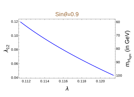
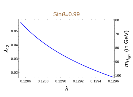
Figure 2: Correspondence between $\lambda=\lambda_{1}=\lambda_{2}$ and $\lambda_{12}$ for low mass region with the light scalar mass varying between 60 GeV $\leq m_{H_{\rm light}}\leq$ 100 GeV, with mixing angle fixed at $\sin\theta=0.9$ (for left panel) and $\sin\theta=0.99$ (for right panel) respectively.

In Fig 2 we show the variation of $\lambda$ and $\lambda_{12}$ for the low mass region. Here we observe that for a variation of the light Higgs mass $m_{H_{\rm light}}=60-100$ GeV, $\lambda$ varies between 0.11 to 0.12, whereas $\lambda_{12}$ varies between 0.12 to 0.04 when $\sin\theta$ is fixed at 0.9. Note here that there is a one-to-one correspondence between $\lambda$ and $\lambda_{12}$, which broadens up once we relax our assumption, i.e. $\lambda_{1}\neq\lambda_{2}$ (see Appendix B). When $\lambda_{12}$ increases, $\lambda$ decreases. There is another point to note here, $\lambda_{12}$ is also present in the triple Higgs vertex, which will control the DM phenomenology to some extent as we will demonstrate. However, we do not have a freedom of choosing it once we know both the Higgs masses and mixing. Self couplings are anyway very difficult to estimate in collider experiments. The analysis above is mainly aimed at showing the legitimacy of the input parameters for the choices of the masses of light Higgs, which we use in our further analysis.

3.2 High mass region

As in the low mass case, the relation between the mass eigenstates and gauge eigenstates for the high mass region can be written as,

$$\left(\begin{array}[]{c}h_{\rm SM}\\ H_{\rm heavy}\end{array}\right)=\left(\begin{array}[]{cc}\cos\theta&-\sin\theta\\ \sin\theta&\cos\theta\end{array}\right)\left(\begin{array}[]{c}\tilde{h}\\ h^{\prime}\end{array}\right).$$ (12)

with the corresponding physical masses given by

$$m_{h_{\rm SM}}^{2} = \lambda_{1}v^{2}+\lambda_{2}u^{2}-\sqrt{(\lambda_{1}v^{2}-\lambda_{2}u^{2})^{2}+\lambda_{12}^{2}u^{2}v^{2}},$$

$$m_{H_{\rm heavy}}^{2} = \lambda_{1}v^{2}+\lambda_{2}u^{2}+\sqrt{(\lambda_{1}v^{2}-\lambda_{2}u^{2})^{2}+\lambda_{12}^{2}u^{2}v^{2}}.$$ (13)

Following the notation we established, we identify $h_{\rm SM}$ as the Higgs discovered at the LHC (with $m_{h_{\rm SM}}=125.7$ GeV) and $m_{h_{\rm SM}}<m_{H_{\rm heavy}}$. Therefore, in this alternate scenario, we work in small $\sin\theta$ limit ($\sin\theta\rightarrow 0$ for decoupling), where $h_{\rm SM}$ is dominantly a scalar doublet and $H_{\rm heavy}$ gets contribution mainly from the scalar singlet $\phi$. This gives us the freedom to choose any mass of the other physical scalar heavier than the observed Higgs mass. To see how the physical masses are related to the input parameters, we recast the couplings as:

$$\lambda_{1} = \frac{m_{h_{\rm SM}}^{2}}{4v^{2}}(1+\cos 2\theta)+\frac{m_{H_{\rm heavy}}^{2}}{4v^{2}}(1-\cos 2\theta),$$ (14)

$$\lambda_{2} = \frac{m_{h_{\rm SM}}^{2}}{4u^{2}}(1-\cos 2\theta)+\frac{m_{H_{\rm heavy}}^{2}}{4u^{2}}(1+\cos 2\theta),$$ (15)

$$\lambda_{12} = \sin 2\theta\frac{m_{H_{\rm heavy}}^{2}-m_{h_{\rm SM}}^{2}}{2uv}.$$ (16)

In order to estimate the couplings in the high mass region, we choose $\sin\theta=0.3$ and 0.001 (values of the mixing angle near the two extremes that are admissible by Higgs data for this region). Using these mixing angles, we find $u,\lambda~{}(=\lambda_{1}=\lambda_{2})$ and $\lambda_{12}$ for various values of $m_{H_{\rm heavy}}$ in Table 3. For larger masses and larger mixing angle, the couplings $\lambda$ and $\lambda_{12}$ are also larger. In Fig. 3, we have presented the correlation between $\lambda$ and $\lambda_{12}$ for the high mass region, fixing $\sin\theta$ at a moderate value of 0.1. For the heavy Higgs mass ranging between $m_{H_{\rm heavy}}$ = 200-1000 GeV, we find that $\lambda$ and $\lambda_{12}$ varies between 0.13-0.21 and 0.025-0.26 respectively. For this case, we also see that for larger $\lambda$, $\lambda_{12}$ is also larger. Again, if we relax the condition of $\lambda_{1}=\lambda_{2}$, the correspondence will be relaxed.

Benchmark Points $m_{H_{\rm heavy}}$ (GeV)	$u$ (GeV)		$\lambda$		$\lambda_{12}$
	$s_{\theta}=0.3$	$s_{\theta}=0.001$	$s_{\theta}=0.3$	$s_{\theta}=0.001$	$s_{\theta}=0.3$	$s_{\theta}=0.001$
200	356.81	391.41	0.1485	0.1306	0.0789	0.0003
400	556.02	782.81	0.2378	0.1306	0.3017	0.0008
600	662.42	1174.21	0.3865	0.1306	0.6138	0.0012
800	700.61	1565.60	0.5947	0.1306	1.0365	0.0016
1000	726.93	1956.98	0.8624	0.1306	1.5751	0.0020

Table 3: Values obtained for $\lambda_{1}=\lambda_{2}=\lambda$ and vev $u$ (in GeV) for some chosen heavy Higgs masses $m_{H_{\rm heavy}}$ = 200, 400, 600 and 1000 GeV and two extreme values of mixing angles $\sin\theta=0.3~{}(0.001),m_{h_{\rm SM}}=125.7$ GeV and $v=246$ GeV.

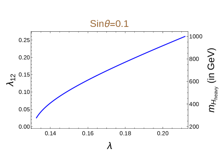
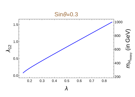
Figure 3: The correlation of $\lambda$ vs $\lambda_{12}$ for high mass region with heavy Higgs ranging between 200 GeV $\leq m_{H_{\rm heavy}}\leq$ 1000 GeV for $\sin\theta=0.1$ (left panel) and $\sin\theta=0.3$ (right panel) respectively.

4 Dark matter relic density and direct search constraints

In this framework the dark sector is kept minimal and consists of a SM singlet fermion $\chi$. A bare Majorana mass term for this fermion is forbidden due to the specific $Z_{4}$ charge as assumed and shown in Table 1. The presence of $Z_{4}$ charged scalar field $\phi$, yields the only coupling $y\phi\bar{\chi^{c}}\chi$, involving the dark fermion as shown in the Lagrangian (Eq. (1)). The mass of dark matter ($M_{\chi}$) appears only through this interaction term, once $\phi$ acquires a vev. At this point, we note that there is no direct renormalisable interaction of the DM with SM fields, which is true for any singlet fermion DM, unless extended to the presence of an additional doublet ArkaniHamed:2005yv ; Mahbubani:2005pt ; DEramo:2007anh ; Enberg:2007rp ; Cynolter:2008ea ; Cohen:2011ec ; Cheung:2013dua ; Restrepo:2015ura ; Calibbi:2015nha ; Freitas:2015hsa ; Bizot:2015zaa ; Cynolter:2015sua . As we have already mentioned, the scalar field ($\phi$), which connects to the dark sector, also plays a crucial role in the neutrino mass generation and the explicit connection between the dark and neutrino sectors will be demonstrated shortly. Thus, prior to the spontaneous breaking of this $Z_{4}$ symmetry, the DM remains massless ($M_{\chi}=0$) and doesn’t have any connection to the visible sector. After SSB, $\phi$ acquires a vev $\langle\phi\rangle$, mixes with SM Higgs doublet ($H$) through the $\phi^{2}H^{\dagger}H$ term and connects the DM with the SM. The two phenomenologically viable scenarios discussed above after SSB, with the additional physical scalar having either lower or higher mass than the physical scalar seen at the LHC, will lead to the following DM couplings through the interactions (following earlier notation):

1. Low mass region (large $\sin\theta$):

$$y\phi\bar{\chi^{c}}\chi = y(-H_{\rm light}\sin\theta+h_{\rm SM}\cos\theta)\bar{\chi^{c}}\chi,$$ (17)

$$= \frac{M_{\chi}}{u}(-H_{\rm light}\sin\theta+h_{\rm SM}\cos\theta)\bar{\chi^{c}}\chi$$

2. High mass region (small $\sin\theta$):

$$y\phi\bar{\chi^{c}}\chi = y(-h_{\rm SM}\sin\theta+H_{\rm heavy}\cos\theta)\bar{\chi^{c}}\chi,$$ (18)

$$= \frac{M_{\chi}}{u}(-h_{\rm SM}\sin\theta+H_{\rm heavy}\cos\theta)\bar{\chi^{c}}\chi.$$

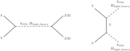
Figure 4: DM ($\chi$) annihilation process that yield relic density of the DM.

In Eq. (17) and (18), we have replaced the DM-scalar coupling by the DM mass as: $y=M_{\chi}/\langle\phi\rangle=M_{\chi}/u$. Note here, we will adhere to the conservative limit of $y\leq 1.0$ from perturbative constraints (see Appendix A) assuming the cut-off scale of the theory to be around $\Lambda\sim 10^{7}$ GeV. The limit on $\Lambda$ in this analysis is obtained satisfying neutrino mass constraints and will be detailed in Sec. 5. The DM will then have an s-channel annihilation through the two physical Higgses to the SM. The other possibility will be to have a t-channel annihilation to the Higgses as shown in the Feynman graphs in Fig. 4. These processes will help the fermion DM to thermally freeze out and we will compute the required values of the DM parameters to satisfy relic density constraints. The second processes (t-channel graphs) will only be feasible when the DM mass is heavier than the Higgs masses. The t-channel graphs will also play an important role to disentangle the annihilation processes to the possible direct search cross-sections that the DM obtains. With non-observation of DM in direct search experiments, such processes are essential to keep the DM model viable.

Here we again mention that the DM analysis has been performed considering $\lambda$ $=\lambda_{1}=\lambda_{2}$ and $m_{h_{\rm SM}}$ fixed at 125.7 GeV as observed by the LHC. Subsequently, we can evaluate $u,\lambda$ and $\lambda_{12}$ once $\sin\theta$ and $m_{H_{\rm light,~{}heavy}}$ are known. Choice of these two parameters ($\sin\theta$ and $m_{H_{\rm light,~{}heavy}}$) is constrained by perturbative unitarity, EW precision data, perturbativity of the couplings along with vacuum stability. We refrain from a detailed discussion in this regard, which can be found in Robens:2015gla ; Robens:2016xkb .

Hence the DM phenomenology is completely dictated by three parameters:

$$M_{\chi},\sin\theta{~{}\rm and~{}}m_{H_{\rm light,~{}heavy}}$$

where $M_{\chi}$ is the mass of the DM, $\sin\theta$ is the mixing angle between two scalars and $m_{H_{\rm light,~{}heavy}}$ is the mass of the additional scalar field. In our analysis, we use micrOMEGAs 4.2.5 Belanger:2008sj to find the relic density and direct search cross sections by scanning the three-fold DM parameter space within the admissible limits.

Depending upon the mass of $m_{H_{\rm light,~{}heavy}}$, our analysis is categorised in two different scenarios: Low mass region ($m_{H_{\rm light}}<m_{h_{\rm SM}}$) and High mass region ($m_{h_{\rm SM}}<m_{H_{\rm heavy}}$) respectively to obtain constraints from DM relic density and non-observation of DM in direct search experiments.

Before we go into the details of the parameter space scan and the associated DM constraints, a few comments are in order. The vev of $\phi$, as is clearly seen from the Lagrangian, will break the $Z_{4}$ symmetry to a remnant $Z_{2}$. The stability of the DM is ensured by this preserved $Z_{2}$ symmetry. The situation of a SM singlet fermion DM that is $Z_{2}$-odd and connected to the SM through the mixing of a scalar singlet (which is even under $Z_{2}$) with SM Higgs has been studied in the literature Kim:2008pp ; Baek:2011aa ; LopezHonorez:2012kv ; Carpenter:2013xra ; Abdallah:2015ter ; Dutra:2015vca ; Buckley:2014fba ; DeSimone:2016fbz ; Arcadi:2017kky . The model we consider here has distinct DM phenomenology, although mostly having similar features. One of the main differences is simply that the dark matter mass is proportional to the vev of the extra scalar $\phi$ (which in turn is related to $\sin\theta$). Another is the absence of the cubic $\phi^{3}$ term in the scalar potential, forbidden by the $Z_{4}$ symmetry in our model, but allowed in the previously studied models where the scalar $\phi$ would be neutral. The cubic term would have altered the triple Higgs vertex, therefore changing the s-channel annihilation for the DM to the Higgs final states and also adding to the freedom of choosing the Higgs masses while keeping the input parameters within admissible range. The $Z_{4}$ symmetry in our model that is essential to connect in our model the DM to the neutrino sector, is therefore further motivated as it simplifies the DM analysis, and makes the model considerably more predictive. The scans performed in the next subsections have been systematized to the requirement of connecting to the neutrino sector.

4.1 Dark matter phenomenology in light Higgs mass region

As has already been mentioned, in this case we assume the second neutral Higgs to be lighter $m_{h_{\rm SM}}>m_{H_{\rm light}}$ with large $\sin\theta$ and of course $m_{h_{\rm SM}}=125.7$ GeV. In Table 4 we list relevant vertices that connects the DM to the visible sector and corresponding vertex factors in terms of parameters $M_{\chi},\sin\theta$ and vevs $u,v$ and couplings $\lambda,\lambda_{12}$ with the assumption of $\lambda_{1}=\lambda_{2}=\lambda$. Note that the couplings are only present in the triple Higgs vertex and they do not show up elsewhere. Also we note again that the the couplings are automatically determined once we choose the light scalar mass and mixing. The vertices are introduced in the code micrOMEGAs Belanger:2008sj for a scan of the parameters to yield correct relic density and direct search observations.

Vertices	Vertex Factor
$H_{\rm light}\chi\chi$	$-y\sin\theta=-(M_{\chi}/u)\sin\theta$
$H_{\rm light}W^{+}W^{-}$	$\frac{2M_{W}^{2}}{v}\cos\theta$
$H_{\rm light}ZZ$	$\frac{2M_{Z}^{2}}{v}\cos\theta$
$H_{\rm light}h_{\rm SM}h_{\rm SM}$	$2\left(\frac{1}{2}v\lambda_{12}c^{3}_{\theta}-3u\lambda c^{2}_{\theta}s_{\theta}+u\lambda_{12}c^{2}_{\theta}s_{\theta}+3v\lambda c_{\theta}s^{2}_{\theta}-v\lambda_{12}c_{\theta}s^{2}_{\theta}-\frac{1}{2}u\lambda_{12}s^{3}_{\theta}\right)$
$h_{\rm SM}\chi\chi$	$y\cos\theta=(M_{\chi}/u)\cos\theta$
$h_{\rm SM}W^{+}W^{-}$	$\frac{2M_{W}^{2}}{v}\sin\theta$
$h_{\rm SM}ZZ$	$\frac{2M_{Z}^{2}}{v}\sin\theta$
$h_{\rm SM}f\overline{f}$	$\frac{m_{f}}{v}\sin\theta$
$h_{\rm SM}H_{\rm light}H_{\rm light}$	$2\left(\frac{1}{2}u\lambda_{12}c^{3}_{\theta}+3v\lambda c^{2}_{\theta}s_{\theta}-v\lambda_{12}c^{2}_{\theta}s_{\theta}+3u\lambda c_{\theta}s^{2}_{\theta}-u\lambda_{12}c_{\theta}s^{2}_{\theta}+\frac{1}{2}v\lambda_{12}s^{3}_{\theta}\right)$

Table 4: Vertices that connect DM to the SM in low mass region. Vertex factors are written assuming $\lambda_{1}=\lambda_{2}=\lambda$.

4.1.1 Relic Density

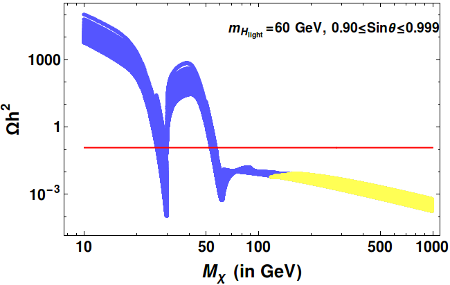
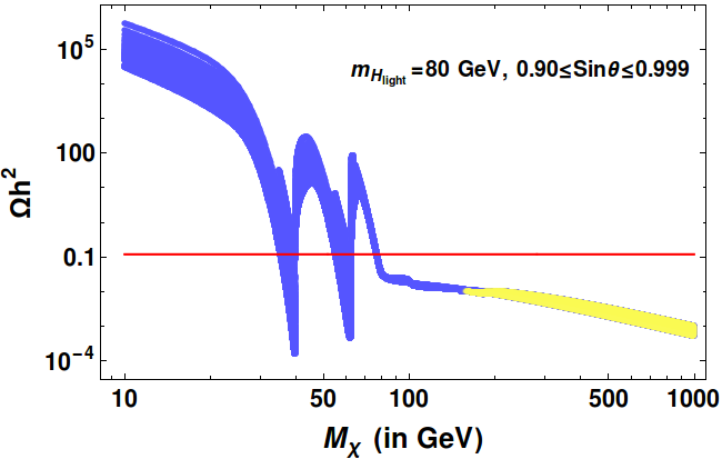
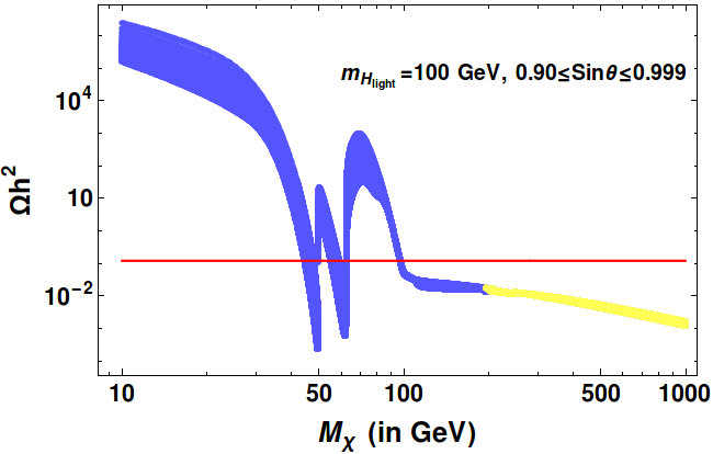
Figure 5: Relic density ($\Omega h^{2}$) of the fermion DM as a function of DM mass $M_{\chi}$ for three different choices of $m_{H_{\rm light}}$=60, 80 and 100 GeV respectively shown in the upper left, right and bottom panel. The Higgs mixing angle is varied between $0.9\leq\sin\theta\leq 0.99$. Yellow region lies outside perturbative limit of coupling $y$ and corresponds to $y>1.0$. Horizontal red line represents observed relic density by Planck data (see Eq. (20)).

The relic density of the DM is inversely proportional to the thermal averaged annihilation cross-section of the DM ($\langle\sigma{\rm v}\rangle$) guided by the relation (assuming $x_{f}\sim 20$):

$$\Omega h^{2}\simeq\frac{2.4\times 10^{-10}~{}{\rm GeV^{-2}}}{\langle\sigma\;{\rm v}\rangle_{{}_{\chi\chi\to SM\;SM}}},$$ (19)

where $\langle\sigma\;{\rm v}\rangle_{{}_{\chi\chi\to SM\;SM}}$ denotes thermal average annihilation cross-section of the DM ($\chi$) to SM final states including the light/heavy Higgs whenever kinematically permissible (as in Feynman graphs in Fig. 4). Note that we obtain the relic density numerically by implementing the model in the code micrOMEGAs Belanger:2008sj .

In Fig. 5, we show the variation of DM relic density as a function of DM mass $M_{\chi}$. In the left, middle and right panel of Fig. 5, the BSM scalar mass $m_{H_{\rm light}}$ is fixed at 60, 80 and 100 GeV respectively. In each panel the blue patch represents the variation of the mixing angle $\sin\theta$ in the range $0.90\leq\sin\theta\leq 0.999$ Robens:2015gla ; Robens:2016xkb . The region between the red horizontal lines represents correct relic density satisfying the PLANCK constraint Ade:2015xua :

$$0.1175\leq\Omega h^{2}\leq 0.1219.$$ (20)

Due to s-channel annihilation of the DM through the two Higgses ($h_{\rm SM}$ and $H_{\rm light}$), in each panel of Fig. 5, we find two resonance regions for $M_{\chi}=m_{h_{\rm SM}}/2$ and $M_{\chi}=m_{H_{\rm light}}/2$, where the relic density drops sharply, intersecting the relic density constraint. In these plots we also observe that, as soon as the dark matter mass becomes comparable (or greater than) with the mass of additional scalar $H_{\rm light}$, the dark matter annihilation is dominantly controlled by the $\chi\chi\rightarrow{H_{\rm light}}{H_{\rm light}}$ process through t- channel graph (see Feynman diagram in Fig. 4). In Fig. 5, we also find that the relic density approaches the constraint when $M_{\chi}\sim m_{H_{\rm light}}$ = 80 and 100 GeV as shown in the right and bottom panel respectively. However for $m_{H_{\rm light}}=60$ GeV, due to large annihilation via $\chi\chi\rightarrow{H_{\rm light}}{H_{\rm light}}$, the only regions which satisfy observed relic density are the resonance regions. Very importantly, we note that the heavy dark matter mass regions are severely constrained by the perturbative limit on coupling $y$; imposing $y>1.0$ (regions marked in yellow), DM masses above $\sim 200$ GeV for light Higgs mass $\sim 100$ GeV are disfavoured. The perturbative limit is even stronger for smaller values of the light Higgs mass. We also note that the DM mass $<m_{h_{\rm SM}}/2$ is constrained by the Higgs invisible decay branching fraction that limits the mixing angle $\sin\theta$, as detailed in Appendix C.

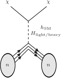
Figure 6: Feynman diagrams for DM to interact with Nucleon.

4.1.2 Direct Search

Direct search of the fermion DM occurs through the t-channel graph mediated by the Higgs portal interactions as shown in Fig. 6. We again compute the direct search cross-sections of the DM through the code micrOMEGAs. The spin-independent Higgs portal interaction includes not just interactions with the light quarks, but also a dominant Higgs-gluon-gluon effective interaction Hisano:2010ct . This gluon contribution arises at loop level, mediated by heavy quarks, and it is implemented in the code by the gluon form factor $f^{(n)}_{T_{g}}=\frac{2}{27}(1-\sum\limits_{q=u,d,s}f^{(n)}_{T_{q}})$ Belanger:2008sj . We use the default form factors of micrOMEGAs with $f^{p}_{T_{u}}=0.0153$, $f^{p}_{T_{d}}=0.0191$ and $f^{p}_{T_{s}}=0.0447$ for proton.

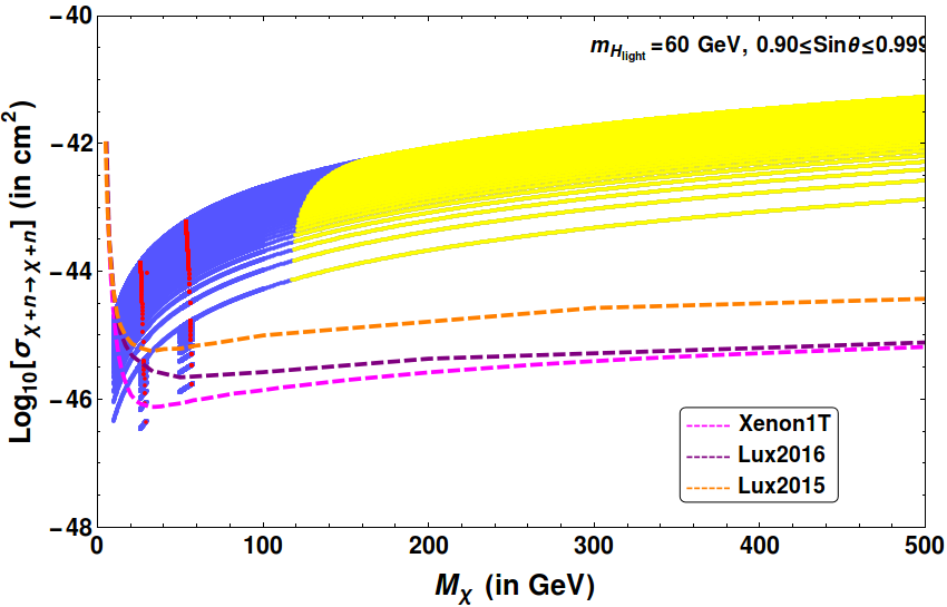
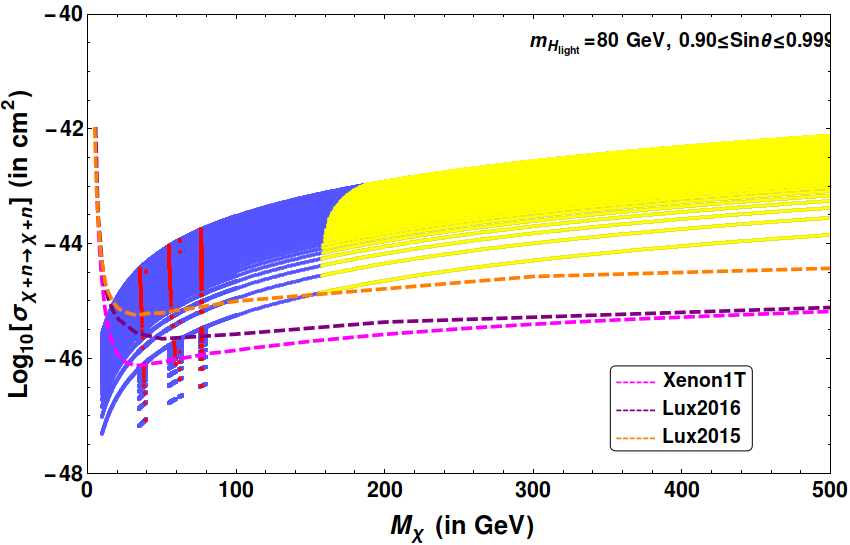
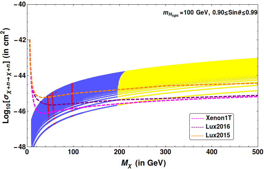
Figure 7: Spin independent direct search cross section as a function of DM mass $M_{\chi}$ for three different choices of $m_{H_{\rm light}}$ = 60, 80 and 100 GeV respectively shown in the upper left, right and bottom panel. In each panel blue patch stands for $0.90\leq\sin\theta\leq 0.999$. Red dots in respective panels satisfy relic density constraints. Bounds from LUX and XENON1T are also shown through dotted/dashed lines. The yellow region corresponds to $y>1.0$ which may violate the perturbative limit.

In Fig. 7, we show spin direct search scattering cross-section of the fermion DM in the low mass region. The plot is drawn as a function of DM mass $M_{\chi}$; for three distinct choices of the BSM scalar mass: $m_{h_{\rm light}}$ = 60 GeV (left), 80 GeV (right) and 100 GeV (bottom) respectively. We consider here the Higgs mixing $\sin\theta$ between 0.90 to 0.999, as we considered previously. The relic density allowed parameter space for the DM in these plots is represented by the dotted red dotted lines appearing in the blue regions. The current experimental bounds from non-observation of DM in direct search experiments from LUX and XENON1T data are shown by dashed lines.

The main outcome of this analysis is to see that the regions which satisfy both relic density and direct search constraints are those in the resonance regions, $M_{\chi}=m_{h_{\rm SM}}/2,m_{H_{\rm light}}/2$ and $M_{\chi}=m_{H_{\rm light}}$. The model is also disfavoured for DM mass beyond $\sim$ 200 GeV, due to the imposition of $y>1.0$ associated with the perturbative limit (see Appendix A). Therefore, the model is quite restrictive in predicting the DM mass from DM constraints. This serves as a key feature to identify the connection to the neutrino sector in an unambiguous way.

4.2 Dark matter phenomenology in heavy Higgs mass region

Now let us turn to DM phenomenology of the heavy Higgs mass region, where we consider $m_{h_{\rm SM}}<m_{H_{\rm heavy}}$ with small $\sin\theta$ and $m_{h_{\rm SM}}=125.7$ GeV. First we note the vertices relevant for DM annihilations and scattering in Table 5 with appropriate vertex factors. This table is similar to Table 4 that corresponds to the low mass region excepting for the flip of notation in the triple Higgs vertices. Again, we parametrise the vertex factors in the limit of $\lambda_{1}=\lambda_{2}=\lambda$, which automatically get determined by the input of the heavy Higgs mass and mixing.

Vertices	Vertex Factor
$h_{\rm SM}\chi\chi$	$-y\sin\theta=-(M_{\chi}/u)\sin\theta$
$h_{\rm SM}W^{+}W^{-}$	$\frac{2M_{W}^{2}}{v}\cos\theta$
$h_{\rm SM}ZZ$	$\frac{2M_{Z}^{2}}{v}\cos\theta$
$h_{\rm SM}f\overline{f}$	$\frac{m_{f}}{v}\cos\theta$
$h_{\rm SM}H_{\rm heavy}H_{\rm heavy}$	$2\left(\frac{1}{2}v\lambda_{12}c^{3}_{\theta}-3u\lambda c^{2}_{\theta}s_{\theta}+u\lambda_{12}c^{2}_{\theta}s_{\theta}+3v\lambda c_{\theta}s^{2}_{\theta}-v\lambda_{12}c_{\theta}s^{2}_{\theta}-\frac{1}{2}u\lambda_{12}s^{3}_{\theta}\right)$
$H_{\rm heavy}\chi\chi$	$y\cos\theta=(M_{\chi}/u)\cos\theta$
$H_{\rm heavy}W^{+}W^{-}$	$\frac{2M_{W}^{2}}{v}\cos\theta$
$H_{\rm heavy}ZZ$	$\frac{2M_{Z}^{2}}{v}\cos\theta$
$H_{\rm heavy}h_{\rm SM}h_{\rm SM}$	$2\left(\frac{1}{2}u\lambda_{12}c^{3}_{\theta}+3v\lambda c^{2}_{\theta}s_{\theta}-v\lambda_{12}c^{2}_{\theta}s_{\theta}+3u\lambda c_{\theta}s^{2}_{\theta}-u\lambda_{12}c_{\theta}s^{2}_{\theta}+\frac{1}{2}v\lambda_{12}s^{3}_{\theta}\right)$

Table 5: Relevant vertices implying DM-SM interactions with vertex factors for high mass region.

4.2.1 Relic Density

In this case relic density is plotted in Fig. 8 for three different values for $m_{H_{\rm heavy}}$, namely 200, 300, 400, and 600 GeV respectively. The mixing angle $\sin\theta$ is varied from 0.001 to 0.3 Robens:2015gla ; Robens:2016xkb . Here also, in each figure, two distinct resonances can be observed at $m_{h}/2$ and $m_{H_{\rm heavy}}/2$. Apart from these resonance regions, for each choice of $m_{H_{\rm heavy}}$, there exists a large allowed range for $M_{\chi}>m_{H_{\rm heavy}}$, which satisfies the observed relic density by Planck data, mainly dominated by the annihilation channel $\chi\chi\rightarrow{H_{\rm heavy}}{H_{\rm heavy}}$. In the high mass region there is a relative large span of the mixing angle (when compared to the low mass region). Another important point is that the triple Higgs vertex is proportional to the additional Higgs mass, and thus for heavy region, that coupling is enhanced. These important differences lead to larger regions being consistent with relic density for $M_{\chi}>m_{H_{\rm heavy}}$, when compared to the low mass case where there was only a small patch of $M_{\chi}\simeq m_{H_{\rm light}}$ for low mass case. In Fig. 8, we have again indicated $y>1.0$ region in yellow, which lies beyond the perturbative limit. This discards a significant part of the relic density allowed parameter space of the model with $M_{\chi}>m_{H_{\rm heavy}}$. We however note that, as the perturbative limit on $y$ depends on the cut-off scale of the theory, we can allow a bit more parameter space by being less strict and imposing instead $y>1.16$, by taking smaller values of $\Lambda\sim 10^{6}$ GeV, which is permissible with neutrino mass limits (as detailed in Section 5).

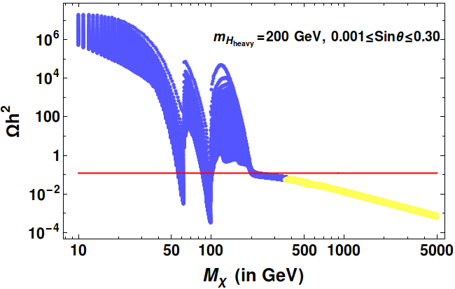
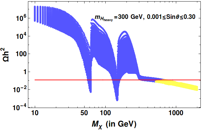
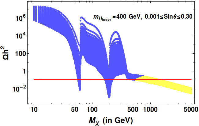
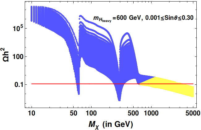
Figure 8: Relic density ($\Omega h^{2}$) obtained as a function of DM mass ($M_{\chi}$) for three different choices of heavy Higgs mass: $m_{H_{\rm Heavy}}$=200, 300, 400 and 600 GeV. Mixing angle is varied between $0.001\leq\sin\theta\leq 0.3$. Horizontal red band represents observed relic density by Planck data. The yellow region corresponds to $y>1.0$ which may violate the perturbative limit.

4.2.2 Direct Search

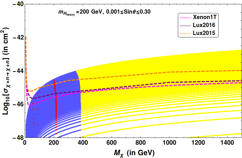
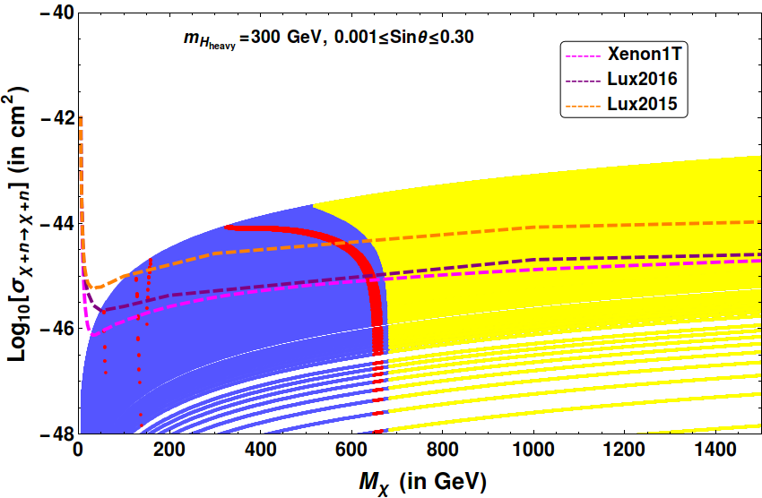
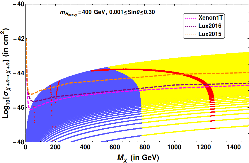
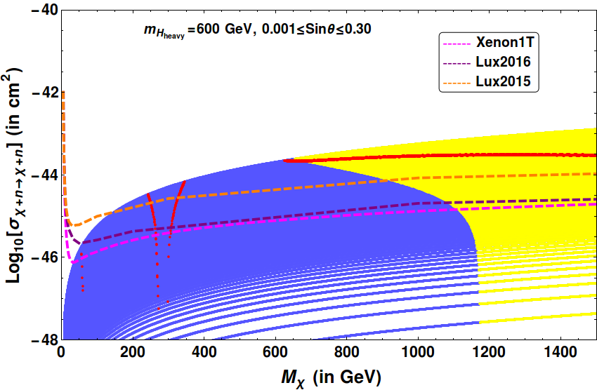
Figure 9: Spin independent direct search cross section as a function of DM mass ($M_{\chi}$) for $m_{H_{\rm Heavy}}$=200, 300, 400 and 600 GeV. The mixing angle is varied between $0.001\leq\sin\theta\leq 0.3$. Red dots in respective panels additionally satisfy relic density constraints. Bounds from XENON1T and LUX data are shown. The yellow region corresponds to $y>1.0$ which may violate the perturbative limit.

The variation of the spin independent direct search scattering cross-section with the DM mass $M_{\chi}$ is plotted in Fig. 9 for heavy Higgs masses: $m_{H_{\rm heavy}}$ = 200, 300, 400 and 600 GeV. The blue region is obtained by scanning all the values of mixing angle in the range of $0.001\leq\sin\theta\leq 0.3$. The red points additionally satisfy relic density constraints for the choice of the specific heavy Higgs mass. Experimental direct search constraints from LUX and XENON data are shown by the dotted lines. Contrary to the low mass region, we see that a significant region of parameter space can be found below the direct search region for a wide range of DM masses. When considering the points allowed by the relic density, we see that for $M_{\chi}\gg m_{H_{\rm heavy}}$ we can satisfy relic density and direct search bounds in this model outside of the resonance regions. This is due to the freedom in choosing a large range of $\sin\theta$ and the annihilation to Higgs final states, which is not constrained by the direct search cross-sections. Obviously, for larger $m_{H_{\rm heavy}}$, the required DM mass to satisfy relic density and direct search bounds is also larger. Unfortunately, for $m_{H_{\rm heavy}}\gtrsim$ 300 GeV, these points mostly fall into the yellow shaded region corresponding to $y>1.0$, which is discarded by perturbative limit.

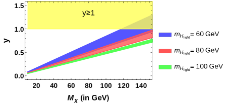
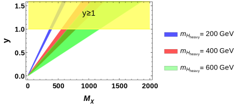
Figure 10: Left: Coupling ($y$) vs DM mass $M_{\chi}$ in the low mass region for $m_{H_{\rm light}}$=60, 80 and 100 GeV with $0.90\leq\sin\theta\leq 0.999$. Right: $y$ vs $M_{\chi}$ for high mass region with $m_{H_{\rm heavy}}$=200, 400, 600 GeV for $0.001\leq\sin\theta\leq 0.3$. The yellow region corresponds to $y>1.0$ which may violate the perturbative limit.

One can easily estimate the required coupling $y$ given a specific choice of the heavy/light Higgs mass. In Fig. 10 we plot $y$ vs $M_{\chi}$ using the relation $y=M_{\chi}/u$ for both low mass (Eq. 9) and high mass (Eq. 14) regions with the assumption $\lambda=\lambda_{1}=\lambda_{2}$. We show the cases of the same choices of the benchmark values of the heavy and light Higgs masses for both high and low mass regions as used in the DM analysis, spanning the admissible range of mixing angle. We see that for larger DM mass, the required coupling $y$ is larger. Also for smaller BSM Higgs mass, the required coupling $y$ is larger given a specific DM mass. The perturbative disallowed region with $y>1.0$ is shown by the yellow band. Therefore, larger values of DM masses are disfavoured by the high coupling $y$ specifically when the BSM Higgs mass is chosen smaller. The implication is that in this model, viable DM masses are mainly those in the resonance regions (as has already been discussed above). For the low mass region, points with $M_{\chi}\simeq m_{H_{\rm light}}$ allowed by the DM constraints have admissible value for $y$ and therefore can be considered, but for the high mass region, allowed points with $M_{\chi}\gg m_{H_{\rm heavy}}$ are disfavoured by imposing $y<1$. Furthermore, for $M_{\chi}<m_{h_{\rm SM}}/2$ Higgs invisible decays constraints severely restrict the allowed values of $\sin\theta$ (see Appendix C).

Mass of the Scalar	$\sin\theta$	$\lambda$	$\lambda_{12}$	$u$ GeV	$y$	$M_{\chi}$ GeV	$\Omega h^{2}$	Log10[$\sigma_{\rm SI}$]$\times 10^{-45}$ cm2
$m_{H_{\rm light}}=$100 GeV	0.993	0.13	0.019	196.99	0.236	46.59	0.118	-46.10
	0.996	0.13	0.011	196.45	0.292	57.46	0.121	-46.15
	0.998	0.13	0.008	196.08	0.496	97.34	0.121	-45.99
	0.999	0.13	0.005	195.89	0.497	97.40	0.119	-46.29
$m_{H_{\rm heavy}}=$200 GeV	0.069	0.133	0.017	389.43	0.154	60	0.122	-46.90
	0.031	0.131	.008	391.01	0.233	91	0.119	-47.23
	0.011	0.131	0.003	391.35	0.552	216	0.121	-47.37
$m_{H_{\rm heavy}}=$400 GeV	0.129	0.150	0.104	723.90	0.083	60	0.120	-46.55
	0.115	0.146	0.091	735.04	0.278	204	0.118	-45.60
$m_{H_{\rm heavy}}=$600 GeV	0.165	0.208	0.248	918.13	0.065	60	0.119	-46.50
	0.093	0.155	0.121	1072.67	0.283	304	0.118	-45.70

Table 6: Some characteristic benchmark points for the model in both low and high mass regions satisfying dark matter relic density and direct search constraints.

In table 6, we have listed some benchmark points from both low and high mass regions that are allowed by DM phenomenology and fulfil the perturbative limit on $y$. The benchmark points lie essentially in the two Higgs resonance regions as discussed. Also it is permissible to have DM mass in the vicinity of the light/heavy Higgs mass (when particularly the heavy Higgs is not too heavy, in order to avoid the perturbative limit).

5 Seesaw mechanism and the connection to dark matter

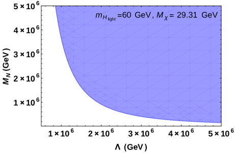
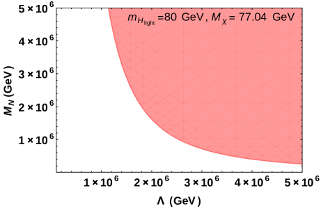
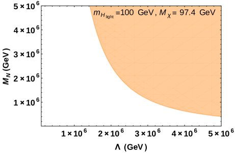
Figure 11: Correlation between right handed neutrino mass $M_{N}$ and cut-off scale $\Lambda$ for $m_{H_{\rm light}}$ = 60, 80 and 100 GeV with corresponding DM masses $M_{\chi}$=29.31, 77.04 and 97.4 GeV respectively satisfying both relic density and direct search constraints.

As has already been mentioned, beyond generating the dark matter mass, the scalar field $\phi$ is also instrumental for generating the Yukawa couplings of the neutrinos which then lead to the light neutrino mass through type-I seesaw. From Eq. (2), the seesaw formula in the present scenario can be written as

$$m_{\nu} = \frac{v^{2}u^{2}}{\Lambda^{2}M_{N}}=\frac{v^{2}}{y^{2}}\frac{(M_{\chi}/\Lambda)^{2}}{M_{N}}.$$ (21)

Recent cosmological observation by Planck suggests that sum of absolute masses of three light neutrinos to be $\sum m_{i}\leq 0.23$ eV Ade:2015xua . Using Eq. (21), the bound on the masses of the light neutrinos can be written as

$$\frac{v^{2}}{y^{2}}\frac{M_{\chi}^{2}}{\Lambda^{2}M_{N}}\leq 0.23~{}{\rm{eV}}.$$ (22)

Therefore, once we have an idea of the DM mass from the relic density and direct search constraints, as we have already obtained in the previous section, we employ Fig. 10 (left and right panels for low and high mass regions respectively) to determine the corresponding Yukawa $y$. The allowed regions for the right handed neutrino mass ($M_{N}$) and cut-off scale of the theory ($\Lambda$) can then be obtained from the above constraint on the combination $\Lambda^{2}M_{N}$ following Eq. (22). For example, in the low mass region, from Fig. 7 we find that with $m_{H_{\rm light}}=60,80$ and 100 GeV both relic density and direct search constraint can be satisfied for DM mass $M_{\chi}$= 29.31, 77.04 and 97.4 GeV respectively. Hence following Eq. 22, we draw a correlation between the right handed neutrino mass $M_{N}$ and cut-off scale $\Lambda$ in Fig. 11. The shaded regions in all the panels are the allowed regions by all constraints. This indicates to the choice of a cut off scale of the model $\Lambda\gtrsim 10^{6}$ GeV as has already been advocated. This in turn then implies that the perturbative limit on the coupling $y$ to be as stringent as $y<1.16$, which we have imposed in the DM analysis (see Appendix A for details). We also note that in the top left figure, DM mass is less than half of SM Higgs mass, which causes the SM Higgs to decay invisibly. The LHC data constrains such a case to limit the mixing $\sin\theta$ (see Appendix C for details), which falls within our chosen range.

Similarly, for high mass region, we draw the similar correlations between right handed neutrino mass and the cut-off scale for different choices of Heavy Higgs mass which unambiguously point out to specific DM masses to satisfy relic density and direct search constraints as given in Fig. 12. Here we have drawn the correlations for DM masses $M_{\chi}$ = 216, 204, 307 GeV respectively (corresponding to $\sin\theta=0.011,~{}0.115,~{}0.119$). For heavier DM mass, the right handed neutrino mass and cut-off scale are also required to be heavier.

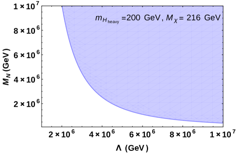
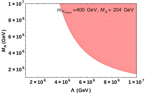
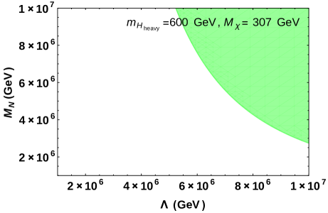
Figure 12: Correlation between right handed neutrino mass $M_{N}$ and cut-off scale $\Lambda$ for successful generation of light neutrino masses for different choices of heavy Higgs mass $m_{H_{\rm heavy}}$ = 200, 400, 600 GeV, which points out to certain definite choices of DM masses as $M_{\chi}$ = 216, 204, 307 GeV respectively (corresponding to $\sin\theta=0.011,~{}0.115,~{}0.119$) to satisfy relic density and direct search constraints together with perturbative bounds.

We consider now in more detail the correlation between neutrino sector and dark matter sector. In the left panel of Fig. 13 we have plotted $u(=M_{\chi}/y)$ vs $\sin\theta$ for $\lambda_{1}=\lambda_{2}=\lambda$ for ranges of $m_{H_{\rm light}}$. Here the magenta, brown and dark red dots represent allowed points satisfying only dark matter relic density (obtained from Fig. 5) for $m_{H_{\rm light}}=100$, 80 and 60 GeV respectively. The blue dots overlaid on each of those 3 lines further satisfy the direct search limit obtained from Fig. 7. Here we find that only $\sin\theta$ values rather close to 1 satisfy the DM constraints. This plot gives an estimate for the scalar singlet vev, $u$, for each low mass case. In the right panel of Fig. 13, we have plotted $u(=M_{\chi}/y)$ as a function of $\Lambda$ (or $M_{N}$) considering $M_{N}=\Lambda$ in Eq. 21 and 22. The purple shaded region represents allowed parameter space in the $u(=M_{\chi}/y)$-$\Lambda(=M_{N})$ plane satisfying upper bound on the sum of light neutrino mass $m_{\nu}\leq 0.23$ eV with $M_{N}=\Lambda$. Here the horizontal blue patches represents the allowed region of $u(=M_{\chi}/y)$ obtained in the left panel (following the analysis of dark matter sector in the previous section). This imposes a stringent constraint on the lower limit of the cut-off scale $\Lambda$ (and RH neutrino mass). Hence for the low mass region (with $m_{H_{\rm light}}=100$, 80 and 60 GeV), we find the lower limit on $\Lambda(M_{N})$ to be $\Lambda(M_{N})\geq 2.2\times 10^{6}$, $1.8\times 10^{6}$ and $1.5\times 10^{6}$ GeV respectively.

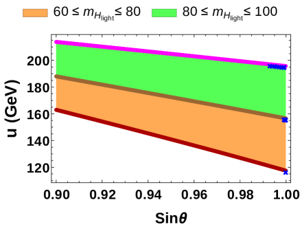
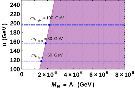
Figure 13: Left panel: $u(=M_{\chi}/y)$ vs $\sin\theta$ plot for $\lambda_{1}=\lambda_{2}=\lambda$ for various range of $m_{H_{\rm light}}$. Here the magenta, brown and dark red dots represent allowed points obtained (from Fig. 5) relic density for $m_{H_{\rm light}}=100$, 80 and 60 GeV. Blue dots on each line are the points allowed by the direct search limit. Right panel: $u(=M_{\chi}/y)$ as a function of $\Lambda$ (or $M_{N}$) considering $M_{N}=\Lambda$ in Eq. 21 and 22. Purple shaded region represents $m_{\nu}\leq 0.23$ eV with $M_{N}=\Lambda$ and the horizontal blue patches represent the allowed region of $u(=M_{\chi}/y)$ obtained the left panel for the specific light Higgs masses. This imposes a stringent constraint on the lower limit of the cut-off scale $\Lambda$ (and RH neutrino mass $M_{N}$).

A similar analysis can be performed for the high mass region. In the left panel of Fig. 14, we have again plotted $u(=M_{\chi}/y)$ against $\sin\theta$ for $\lambda_{1}=\lambda_{2}=\lambda$ for various range of $200\leq m_{H_{\rm heavy}}\leq 400$ GeV and $400\leq m_{H_{\rm heavy}}\leq 600$ GeV as depicted by orange and green shaded regions. In this panel the magenta, brown and dark red dots represents the allowed points satisfying correct dark matter relic density as given in Fig. 8 for $m_{H_{\rm heavy}}=200$, 400 and 600 GeV respectively. Blue dots additionally satisfy direct search constraints as obtained following Fig. 9. Here a relatively large region of $\sin\theta$ satisfies all the DM constraints representing a wide range for scalar singlet vev $u$. In the right panel of Fig. 14, we have again plotted $u(=M_{\chi}/y)$ as a function of $\Lambda$ (or $M_{N}$) considering $M_{N}=\Lambda$ in Eq. 21 and 22 for the high mass region. The purple shaded region represents allowed parameter space in the $u(=M_{\chi}/y)$-$\Lambda(=M_{N})$ plane satisfying the upper bound on the sum of light neutrino mass $m_{\nu}\leq 0.23$ eV with the consideration $M_{N}=\Lambda$. In this right panel, horizontal shaded regions illustrated in blue (for $m_{H_{\rm heavy}}=200$, 400 and 600 GeV) represent the allowed regions for $u(=M_{\chi}/y)$ obtained from the left panel satisfying correct dark phenomenology. From the intercepting regions once again we can obtain the corresponding lower limit on $\Lambda$ (and $M_{N}$). Here we find a relatively wider lower limit for $\Lambda(M_{N})\geq 3.4\times 10^{6}$, (5.0-5.4)$\times 10^{6}$ and (5.64-7.1)$\times 10^{6}$ GeV for $m_{H_{\rm heavy}}=200$, 400 and 600 GeV respectively due to due larger allowed region for $\sin\theta$ (and hence corresponding $u$ in the left panel).

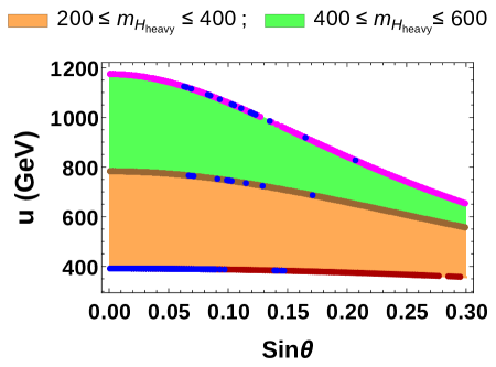
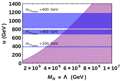
Figure 14: Left panel: $u(=M_{\chi}/y)$ vs $\sin\theta$ plot for $\lambda_{1}=\lambda_{2}=\lambda$ for $200\leq m_{H_{\rm heavy}}\leq 400$ GeV (orange shaded region) and $400\leq m_{H_{\rm heavy}}\leq 600$ GeV (green shaded region) respectively. Here the magenta, brown and deep red dots represent allowed points obtained (from Fig. 8) relic density only, for $m_{H_{\rm light}}=100$, 80 and 60 GeV. Blue dots on each line are actual allowed points which also satisfy direct search limit. Right panel: $u(=M_{\chi}/y)$ as a function of $\Lambda$ (or $M_{N}$) considering $M_{N}=\Lambda$ in Eq. 21 and 22. Purple shaded region represents $m_{\nu}\leq 0.23$ eV with $M_{N}=\Lambda$ and the horizontal blue patch represents the allowed region of $u(=M_{\chi}/y)$ obtained the left panel for the specific heavy Higgs masses. This imposes a constraint on the lower limit of the cut-off scale $\Lambda$ (and RH neutrino mass $M_{N}$).

Now if we compare the left panels of Fig. 13 and 14 we find that for low mass region, only $\sin\theta$ values close to 1 (denoted by the blue dots for $m_{H_{\rm light}}$= 100, 80 and 60 GeV respectively) satisfy direct search constraint. Hence the lighter Higgs is dominantly scalar singlet and s-channel contribution to the DM annihilation almost vanishes and t-channel diagrams dominantly contributes both in relic density and direct search constraints. In contrast, for the high mass region the bound on $\sin\theta$ is a bit relaxed (also denoted by the blue dots for $m_{H_{\rm heavy}}$= 200, 400 and 600 GeV respectively) in order to satisfy both relic density and direct search constraints. This eventually leads to the fact that for low mass region, for a specific value of $m_{H_{\rm light}}$ the lower limit for the cut-off scale $\Lambda$ (or RH neutrino mass $M_{N}$) is tightly constrained as evident from the right panel of Fig. 13. But for the high mass region, due to the large allowed range for $\sin\theta$, for a fixed value of $m_{H_{\rm heavy}}$ we have a wide allowed range for the lower limit for the cut-off scale $\Lambda$ (or RH neutrino mass $M_{N}$). This is shown in the right panel of Fig. 14.

6 Summary and Conclusions

We have successfully constructed a framework where seesaw and DM sectors are related to each other by a common scalar mediator. The relation is mainly restricted by the vev of the scalar singlet field which yields both DM mass and controls the neutrino Yukawa coupling in the type-I seesaw within an effective theory framework. The first part of the framework described above constrains the DM mass from relic density and direct search constraints, depending on the mass of mixing associated with the additional Higgs. Given this information, we have explored the correlation between the right handed neutrino masses with the cut-off scale present in the theory. The main success of the set-up is to establish the correlation between DM sector and neutrino sector in a coherent manner. The scenario naturally accommodates two Higgses, one of which can be identified with the Higgs discovered at the LHC. We study both the cases where the additional Higgs field (other than the SM one) is heavier and lighter than the SM Higgs. We find that with the second Higgs as the lighter than the SM Higgs, the allowed DM phenomenology restricts DM $\sim m_{H_{\rm light}}$. On the heavy Higgs region, this connection is little relaxed as a larger region of allowed parameter space is possible for DM. In either cases, there is a prediction for $M_{N}$ and $\Lambda$ to be larger than $10^{6}$ GeV. For simplicity, here we consider the quartic couplings of the two scalars present in the theory as same. The analysis can easily be extended for different values of these couplings, which would yield an extended parameter space (as hinted in the Appendix B).

Very importantly we note that as the coupling $y$ of the scalar mediator to the DM in this model is determined directly by DM mass, the perturbative limit on this coupling reduces the allowed parameter space of the model. The limit on the cut off scale $\Lambda\gtrsim 10^{6}$ GeV, indicates that $y\leq 1.16$ to be within perturbative limit. This explicitly excludes very high DM masses, which in the heavy Higgs region would otherwise satisfy both relic density and direct search constraints. This therefore enhances the predictivity of the model.

As we have already stated, the choice of the dark sector was chosen as a specific example only, and one may do a similar model building exercise to connect seesaw mechanism to some other DM sector. On the other hand, the correlation requires the knowledge of the heavy or light Higgs mass and its mixing with the SM Higgs doublet, which is difficult to find at the current status of collider search experiment. As our framework involves the two heavy scales, namely the RH neutrino mass $M_{N}$ and the cut-off scale $\Lambda$, it would be interesting to find an UV complete construction, although this is beyond the scope of the current work and requires involvement of more fields and symmetry.

Appendix A Perturbative limit on coupling $y$

With the Lagrangian term for the interaction between the dark matter fermion and the scalar given by:

$$\mathcal{L}_{Yuk}=-y\phi\bar{\chi}^{c}\chi~{},$$

the perturbative limit on $y$ at any scale is expected to satisfy $y<\sqrt{4\pi}$. Hence, we should have $y(\Lambda)<\sqrt{4\pi}$, where $y(\Lambda)$ is the coupling at the cut off scale $\Lambda$ of the theory. Now it turns out from the simplified analysis (where we take $\Lambda=M_{N}$) that $\Lambda$ has a lower bound, $\Lambda\gtrsim 10^{6}$ GeV, obtained mainly from neutrino mass limit with a suitable heavy/light Higgs mass to satisfy the DM constraints (see Figs. 11 and 12).

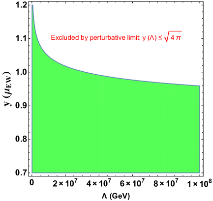
Figure 15: Perturbative limit on the $y$ coupling at electroweak scale $y(\mu_{EW})$ assuming $y(\Lambda)=\sqrt{4\pi}$ as a function of the cut-off scale $\Lambda$. Green region below the curve is allowed by the limit. The range of $\Lambda$ has been chosen from that of our analysis to satisfy neutrino mass limit.

Therefore, in order to keep the $y$ coupling within the perturbative limit near the cut-off scale $\Lambda=M_{N}$, we need to consider suitable value of $y$ at low scale. Below we employ the Renormalisation Group (RG) running of $y$ to evaluate the constraint on it at the electroweak scale. The RG equation for $y$ is Bonilla:2015kna given by:

$$\frac{dy}{dt}=\frac{6}{16\pi^{2}}~{}y^{3},$$ (23)

where $t=\ln\mu$, with $\mu$ denoting the energy scale. Following our convention used in the analysis, $t_{EW}=\ln(v_{EW})=\ln(174)=5.16$, the solution of above equation will be given by:

$$\int_{y_{0}=y(\mu_{EW})}^{y(\Lambda)}\frac{dy}{y^{3}}=\int_{t_{EW}}^{\Lambda}\frac{6}{16\pi^{2}}dt~{},$$ (24)

$$\implies y_{0}=y(\mu_{EW})=1.05,~{}~{}~{}~{}\rm{for}~{}~{}~{}\Lambda=10^{7}~{}~{}GeV,$$

$$\implies y_{0}=y(\mu_{EW})=1.16,~{}~{}~{}~{}\rm{for}~{}~{}~{}\Lambda=10^{6}~{}~{}GeV.$$ (25)

A variation of maximum allowed $y$ at electroweak scale from perturbative limit as a function of cut off scale $\Lambda$ is shown in Fig. 15 as well. The range of $\Lambda$ has been chosen from that of our analysis to satisfy neutrino mass limit. The green region under the curve provides allowed values $y$.

Appendix B The case of having $\lambda_{1}\neq\lambda_{2}$

In the previous analysis we have considered $\lambda_{1}=\lambda_{2}$ for simplicity. However, one can easily extend the analysis by considering $\lambda_{1}\neq\lambda_{2}$ for both low and high mass regions. To facilitate comparison with the previous results, we parametrise $\lambda_{1}=\kappa\lambda_{2}$ and briefly outline the possible changes. For low mass region, using Eq. (9) - (10) and $\lambda_{1}=\kappa\lambda_{2}$, we find,

$$u^{2}=\kappa v^{2}\frac{m_{H_{\rm light}}^{2}(1-\cos 2\theta)+m_{h_{\rm SM}}^{2}(1+\cos 2\theta)}{m_{H_{\rm light}}^{2}(1+\cos 2\theta)+m_{h_{\rm SM}}^{2}(1-\cos 2\theta)}$$ (26)

and the relevant modified vertex factors are given by

$$H_{\rm light}h_{\rm SM}h_{\rm SM} : 2\left(\frac{1}{2}v\lambda_{12}c^{3}_{\theta}-3u\lambda_{2}c^{2}_{\theta}s_{\theta}+u\lambda_{12}c^{2}_{\theta}s_{\theta}+3v\lambda_{1}c_{\theta}s^{2}_{\theta}-v\lambda_{12}c_{\theta}s^{2}_{\theta}-\frac{1}{2}u\lambda_{12}s^{3}_{\theta}\right),$$

$$= 2\left(\frac{1}{2}v\lambda_{12}c^{3}_{\theta}-3u\frac{\lambda_{1}}{\kappa}c^{2}_{\theta}s_{\theta}+u\lambda_{12}c^{2}_{\theta}s_{\theta}+3v\lambda_{1}c_{\theta}s^{2}_{\theta}-v\lambda_{12}c_{\theta}s^{2}_{\theta}-\frac{1}{2}u\lambda_{12}s^{3}_{\theta}\right),$$

$$h_{\rm SM}H_{\rm light}H_{\rm light} : 2\left(\frac{1}{2}u\lambda_{12}c^{3}_{\theta}+3v\lambda_{1}c^{2}_{\theta}s_{\theta}-v\lambda_{12}c^{2}_{\theta}s_{\theta}+3u\lambda_{2}c_{\theta}s^{2}_{\theta}-u\lambda_{12}c_{\theta}s^{2}_{\theta}+\frac{1}{2}v\lambda_{12}s^{3}_{\theta}\right),$$

$$= 2\left(\frac{1}{2}u\lambda_{12}c^{3}_{\theta}+3v\lambda_{1}c^{2}_{\theta}s_{\theta}-v\lambda_{12}c^{2}_{\theta}s_{\theta}+3u\frac{\lambda_{1}}{\kappa}c_{\theta}s^{2}_{\theta}-u\lambda_{12}c_{\theta}s^{2}_{\theta}+\frac{1}{2}v\lambda_{12}s^{3}_{\theta}\right).$$

Similarly, using Eq. (14)-(15) for high mass region, we obtain

$$u^{2}=\kappa v^{2}\frac{m_{h_{\rm SM}}^{2}(1-\cos 2\theta)+m_{H_{\rm heavy}}^{2}(1+\cos 2\theta)}{m_{h_{\rm SM}}^{2}(1+\cos 2\theta)+m_{H_{\rm heavy}}^{2}(1-\cos 2\theta)},$$ (27)

whereas the modified vertices are given by

$$h_{\rm SM}H_{\rm heavy}H_{\rm heavy} : 2\left(\frac{1}{2}v\lambda_{12}c^{3}_{\theta}-3u\lambda_{2}c^{2}_{\theta}s_{\theta}+u\lambda_{12}c^{2}_{\theta}s_{\theta}+3v\lambda_{1}c_{\theta}s^{2}_{\theta}-v\lambda_{12}c_{\theta}s^{2}_{\theta}-\frac{1}{2}u\lambda_{12}s^{3}_{\theta}\right),$$

$$= 2\left(\frac{1}{2}v\lambda_{12}c^{3}_{\theta}-3u\frac{\lambda_{1}}{\kappa}c^{2}_{\theta}s_{\theta}+u\lambda_{12}c^{2}_{\theta}s_{\theta}+3v\lambda_{1}c_{\theta}s^{2}_{\theta}-v\lambda_{12}c_{\theta}s^{2}_{\theta}-\frac{1}{2}u\lambda_{12}s^{3}_{\theta}\right),$$

$$H_{\rm heavy}h_{\rm SM}h_{\rm SM} : 2\left(\frac{1}{2}u\lambda_{12}c^{3}_{\theta}+3v\lambda_{1}c^{2}_{\theta}s_{\theta}-v\lambda_{12}c^{2}_{\theta}s_{\theta}+3u\lambda_{2}c_{\theta}s^{2}_{\theta}-u\lambda_{12}c_{\theta}s^{2}_{\theta}+\frac{1}{2}v\lambda_{12}s^{3}_{\theta}\right),$$

$$= 2\left(\frac{1}{2}u\lambda_{12}c^{3}_{\theta}+3v\lambda_{1}c^{2}_{\theta}s_{\theta}-v\lambda_{12}c^{2}_{\theta}s_{\theta}+3u\frac{\lambda_{1}}{\kappa}c_{\theta}s^{2}_{\theta}-u\lambda_{12}c_{\theta}s^{2}_{\theta}+\frac{1}{2}v\lambda_{12}s^{3}_{\theta}\right).$$

These modified expressions for the vev of the additional scalar and Higgs portal vertices essentially alters the DM phenomenology.

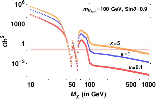
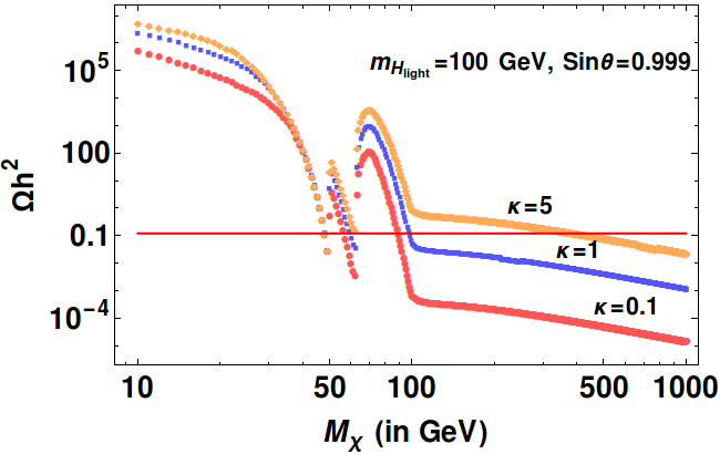
Figure 16: Relic density vs DM mass for various $\kappa(=\lambda_{1}/\lambda_{2})$ values in the low mass region. Here, orange, blue and red dotted lines stands for $\kappa=5$, $\kappa=1$ and $\kappa=0.1$ respectively.

Now, in Fig. 16 and 17, incorporating $\lambda_{1}\neq\lambda_{2}$ we have plotted the variation of relic density as a function of the DM mass ($M_{\chi}$) for low and high mass regions respectively. We observe that as we alter $\kappa$, the Higgs portal coupling also get modified. Here a smaller value of effective coupling (when $\kappa=\lambda_{1}/\lambda_{2}>1$) indicates larger relic density and a larger effective coupling (when $\kappa=\lambda_{1}/\lambda_{2}<1$) indicates smaller relic density compared to $\kappa=1$ case for obvious reasons. This is depicted by the orange ($\kappa=5$), blue ($\kappa=1$) and red ($\kappa=0.1$) dotted lines respectively for all panels in Fig. 16 and 17. While in the low mass DM region only resonance regions satisfy DM constraints, the effect of this change (in terms of $\kappa$) is much more pronounced when the annihilation opens to the other light (or heavy) Higgs for $M_{\chi}>m_{H_{\rm light}}$ (or $m_{H_{\rm heavy}}$). This basically lead to a much larger allowed (by both relic density and Direct search constraints) parameter space specifically in the high DM mass region.

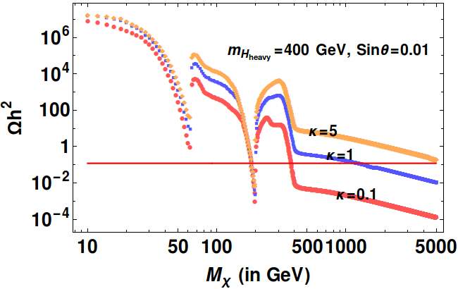
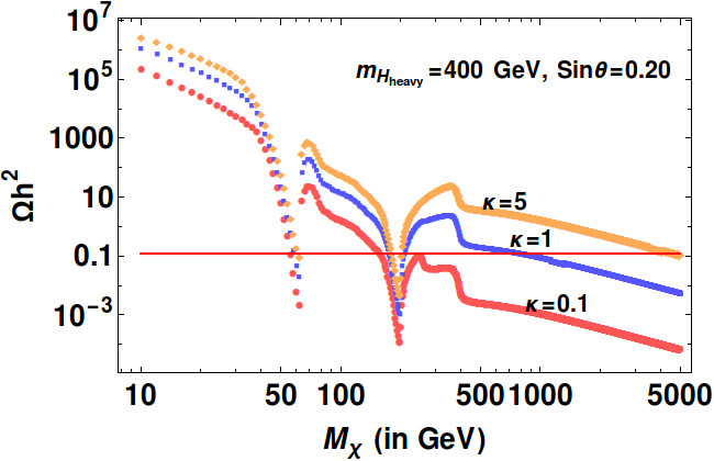
Figure 17: Relic density vs DM mass for various $\kappa(=\lambda_{1}/\lambda_{2})$ values in the high mass region. Here, orange, blue and red dotted lines stands for $\kappa=5$, $\kappa=1$ and $\kappa=0.1$ respectively.

Appendix C Higgs invisible decay constraints

When the DM mass ($M_{\chi}$) is smaller than the SM Higgs mass with $M_{\chi}<m_{h_{\rm SM}}/2$, then SM Higgs can decay to DM and this will contribute to the invisible Higgs decay width. Observations at LHC for the SM Higgs constrains such invisible branching fraction as $Br(h\rightarrow inv)<0.24$  Tanabashi:2018oca . This can be interpreted in terms of invisible decay width as follows:

$$Br(h\to inv.) <0.24$$

$$\frac{\Gamma(h\rightarrow inv.)}{\Gamma(h\rightarrow SM)+\Gamma(h\rightarrow inv.)} <0.24,$$ (28)

where the Higgs decay width to SM is constrained as $\Gamma(h\to SM)=4.2$ MeV (with mass $m_{h_{\rm SM}}=125.7~{}{\rm GeV}$) at the LHC. This limits the invisible decay width as,

$$\Gamma(h\rightarrow inv.)<1.32~{}\rm~{}MeV~{}.$$ (29)

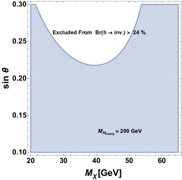
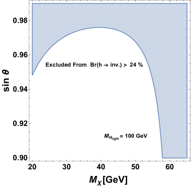
Figure 18: Invisible Higgs decay constraint for $M_{\chi}<m_{h_{\rm SM}}/2$ as a function of scalar mixing angle $\sin\theta$ and DM mass. Left panel shows the case for heavy Higgs mass region with $M_{H_{\rm heavy}}=200$ GeV. Right panel shows the case of light Higgs mass with $M_{H_{\rm light}}=100$ GeV. The shaded region is allowed while the white region is discarded.

The invisible Higgs decay width to DM can be easily calculated:

$$\Gamma_{h\to\chi\chi}=\frac{1}{8\pi}(y\sin\theta)^{2}m_{h_{\rm SM}}~{}~{}\Big{(}1-\frac{4M_{\chi}^{2}}{m_{h_{\rm SM}}^{2}}\Big{)}^{\frac{3}{2}}~{}~{}\Theta(m_{h_{\rm SM}}-2M_{\chi})$$

$$\implies\Gamma_{h\to\chi\chi}=\frac{1}{8\pi}(\frac{M_{\chi}}{u}\sin\theta)^{2}m_{h_{\rm SM}}~{}~{}\Big{(}1-\frac{4M_{\chi}^{2}}{m_{h_{\rm SM}}^{2}}\Big{)}^{\frac{3}{2}}~{}~{}\Theta(m_{h_{SM}}-2M_{\chi}),$$ (30)

where in the above expression, we use the coupling of SM Higgs to DM as $y\sin\theta$ which is valid for the heavy Higgs mass region. A similar expression for the light mass region can be obtained. Invisible Higgs decay constraint will then put a limit on the mixing angle $\sin\theta$. In Fig. 18, we show the limit on $\sin\theta$ in both Heavy Higgs mass region with $M_{H_{\rm heavy}}=200$ GeV in left and light Higgs mass region with $M_{H_{\rm light}}=100$ GeV. The shaded region is allowed while the white region is discarded. The left plot shows that in the high mass region, excepting for the large values of $\sin\theta\sim 0.3$, the small mixing limit is okay with invisible Higgs branching fraction. Light Higgs region is more constrained with larger $\sin\theta\sim 0.99$ being allowed.

References

- (1) D. O. Caldwell and R. N. Mohapatra, Phys. Rev. D 48, 3259 (1993); R. N. Mohapatra and A. Perez-Lorenzana, Phys. Rev. D 67, 075015 (2003) [hep-ph/0212254]; L. M. Krauss, S. Nasri and M. Trodden, Phys. Rev. D 67, 085002 (2003) [hep-ph/0210389]; E. Ma, Phys. Rev. D 73, 077301 (2006) [hep-ph/0601225]; T. Asaka, S. Blanchet and M. Shaposhnikov, Phys. Lett. B 631, 151 (2005) [hep-ph/0503065]; C. Boehm, Y. Farzan, T. Hambye, S. Palomares-Ruiz and S. Pascoli, Phys. Rev. D 77, 043516 (2008) [hep-ph/0612228]; J. Kubo, E. Ma and D. Suematsu, Phys. Lett. B 642, 18 (2006) [hep-ph/0604114]; E. Ma, Mod. Phys. Lett. A 21, 1777 (2006) [hep-ph/0605180]; T. Hambye, K. Kannike, E. Ma and M. Raidal, Phys. Rev. D 75, 095003 (2007) [hep-ph/0609228]; M. Lattanzi and J. W. F. Valle, Phys. Rev. Lett. 99, 121301 (2007) [arXiv:0705.2406 [astro-ph]]; E. Ma, Phys. Lett. B 662, 49 (2008) [arXiv:0708.3371 [hep-ph]]; R. Allahverdi, B. Dutta and A. Mazumdar, Phys. Rev. Lett. 99, 261301 (2007) [arXiv:0708.3983 [hep-ph]]; P. H. Gu and U. Sarkar, Phys. Rev. D 77, 105031 (2008) [arXiv:0712.2933 [hep-ph]]; N. Sahu and U. Sarkar, Phys. Rev. D 78, 115013 (2008) [arXiv:0804.2072 [hep-ph]]; C. Arina, F. Bazzocchi, N. Fornengo, J. C. Romao and J. W. F. Valle, Phys. Rev. Lett. 101, 161802 (2008) [arXiv:0806.3225 [hep-ph]]; M. Aoki, S. Kanemura and O. Seto, Phys. Rev. Lett. 102, 051805 (2009) [arXiv:0807.0361 [hep-ph]]; E. Ma and D. Suematsu, Mod. Phys. Lett. A 24, 583 (2009) [arXiv:0809.0942 [hep-ph]]; P. H. Gu, M. Hirsch, U. Sarkar and J. W. F. Valle, Phys. Rev. D 79, 033010 (2009) [arXiv:0811.0953 [hep-ph]]; M. Aoki, S. Kanemura and O. Seto, Phys. Rev. D 80, 033007 (2009) [arXiv:0904.3829 [hep-ph]]; P. H. Gu, Phys. Rev. D 81, 095002 (2010) [arXiv:1001.1341 [hep-ph]]; M. Hirsch, S. Morisi, E. Peinado and J. W. F. Valle, Phys. Rev. D 82, 116003 (2010) [arXiv:1007.0871 [hep-ph]]; J. N. Esteves, F. R. Joaquim, A. S. Joshipura, J. C. Romao, M. A. Tortola and J. W. F. Valle, Phys. Rev. D 82, 073008 (2010) [arXiv:1007.0898 [hep-ph]]; S. Kanemura, O. Seto and T. Shimomura, Phys. Rev. D 84, 016004 (2011) [arXiv:1101.5713 [hep-ph]]; M. Lindner, D. Schmidt and T. Schwetz, Phys. Lett. B 705, 324 (2011) [arXiv:1105.4626 [hep-ph]]; F. X. Josse-Michaux and E. Molinaro, Phys. Rev. D 84, 125021 (2011) [arXiv:1108.0482 [hep-ph]]. D. Schmidt, T. Schwetz and T. Toma, Phys. Rev. D 85, 073009 (2012) [arXiv:1201.0906 [hep-ph]]; D. Borah and R. Adhikari, Phys. Rev. D 85, 095002 (2012) [arXiv:1202.2718 [hep-ph]]; Y. Farzan and E. Ma, Phys. Rev. D 86, 033007 (2012) [arXiv:1204.4890 [hep-ph]]; W. Chao, M. Gonderinger and M. J. Ramsey-Musolf, Phys. Rev. D 86, 113017 (2012) [arXiv:1210.0491 [hep-ph]]; M. Gustafsson, J. M. No and M. A. Rivera, Phys. Rev. Lett. 110, no. 21, 211802 (2013) Erratum: [Phys. Rev. Lett. 112, no. 25, 259902 (2014)] [arXiv:1212.4806 [hep-ph]]; M. Blennow, M. Carrigan and E. Fernandez Martinez, JCAP 1306, 038 (2013) [arXiv:1303.4530 [hep-ph]]; S. S. C. Law and K. L. McDonald, JHEP 1309, 092 (2013) [arXiv:1305.6467 [hep-ph]]; A. E. Carcamo Hernandez, I. de Medeiros Varzielas, S. G. Kovalenko, H. Päs and I. Schmidt, Phys. Rev. D 88 (2013) no.7, 076014 [arXiv:1307.6499 [hep-ph]]; D. Restrepo, O. Zapata and C. E. Yaguna, JHEP 1311, 011 (2013) [arXiv:1308.3655 [hep-ph]]; S. Chakraborty and S. Roy, JHEP 1401, 101 (2014) [arXiv:1309.6538 [hep-ph]]; A. Ahriche, C. S. Chen, K. L. McDonald and S. Nasri, Phys. Rev. D 90, 015024 (2014) [arXiv:1404.2696 [hep-ph]]; S. Kanemura, T. Matsui and H. Sugiyama, Phys. Rev. D 90, 013001 (2014) [arXiv:1405.1935 [hep-ph]]; W. C. Huang and F. F. Deppisch, Phys. Rev. D 91, 093011 (2015) [arXiv:1412.2027 [hep-ph]]; I. de Medeiros Varzielas, O. Fischer and V. Maurer, JHEP 1508 (2015) 080 [arXiv:1504.03955 [hep-ph]]; B. L. Sánchez-Vega and E. R. Schmitz, Phys. Rev. D 92, 053007 (2015) [arXiv:1505.03595 [hep-ph]]; S. Fraser, C. Kownacki, E. Ma and O. Popov, Phys. Rev. D 93, no. 1, 013021 (2016) [arXiv:1511.06375 [hep-ph]]; R. Adhikari, D. Borah and E. Ma, Phys. Lett. B 755 (2016) 414 [arXiv:1512.05491 [hep-ph]]; A. Ahriche, K. L. McDonald, S. Nasri and I. Picek, Phys. Lett. B 757, 399 (2016) [arXiv:1603.01247 [hep-ph]]; D. Aristizabal Sierra, C. Simoes and D. Wegman, JHEP 1606 (2016) 108 [arXiv:1603.04723 [hep-ph]]. W. B. Lu and P. H. Gu, JCAP 1605, no. 05, 040 (2016) [arXiv:1603.05074 [hep-ph]]; S. Y. Ho, T. Toma and K. Tsumura, Phys. Rev. D 94, no. 3, 033007 (2016) [arXiv:1604.07894 [hep-ph]]; M. Escudero, N. Rius and V. Sanz, Eur. Phys. J. C 77, no. 6, 397 (2017) [arXiv:1607.02373 [hep-ph]]; C. Bonilla, E. Ma, E. Peinado and J. W. F. Valle, Phys. Lett. B 762, 214 (2016) [arXiv:1607.03931 [hep-ph]]; D. Borah and A. Dasgupta, JCAP 1612, no. 12, 034 (2016) [arXiv:1608.03872 [hep-ph]]. A. Biswas, S. Choubey and S. Khan, JHEP 1609, 147 (2016) [arXiv:1608.04194 [hep-ph]]; I. M. Hierro, S. F. King and S. Rigolin, Phys. Lett. B 769, 121 (2017) [arXiv:1609.02872 [hep-ph]]; S. Bhattacharya, S. Jana and S. Nandi, Phys. Rev. D 95 (2017) no.5, 055003 [arXiv:1609.03274 [hep-ph]]; S. Chakraborty and J. Chakrabortty, JHEP 1710, 012 (2017) [arXiv:1701.04566 [hep-ph]]; S. Bhattacharya, N. Sahoo and N. Sahu, Phys. Rev. D 96, no. 3, 035010 (2017) [arXiv:1704.03417 [hep-ph]]; S. Y. Ho, T. Toma and K. Tsumura, JHEP 1707, 101 (2017) [arXiv:1705.00592 [hep-ph]]; P. Ghosh, A. K. Saha and A. Sil, Phys. Rev. D 97, no. 7, 075034 (2018) [arXiv:1706.04931 [hep-ph]]; D. Nanda and D. Borah, arXiv:1709.08417 [hep-ph]; N. Narendra, N. Sahoo and N. Sahu, arXiv:1712.02960 [hep-ph]; N. Bernal, A. E. Cárcamo Hernández, I. de Medeiros Varzielas and S. Kovalenko, JHEP 1805 (2018) 053 [arXiv:1712.02792 [hep-ph]]; D. Borah, B. Karmakar and D. Nanda, arXiv:1805.11115 [hep-ph].
- (2) P. Minkowski, Phys. Lett. B 67, 421 (1977).
- (3) M. Gell-Mann, P. Ramond and R. Slansky, Conf. Proc. C 790927, 315 (1979) [arXiv:1306.4669 [hep-th]].
- (4) R. N. Mohapatra and G. Senjanovic, Phys. Rev. Lett. 44, 912 (1980).
- (5) J. Schechter and J. W. F. Valle, Phys. Rev. D 22, 2227 (1980).
- (6) L. Calibbi, A. Crivellin and B. Zaldívar, Phys. Rev. D 92, no. 1, 016004 (2015) [arXiv:1501.07268 [hep-ph]].
- (7) I. de Medeiros Varzielas and O. Fischer, JHEP 1601, 160 (2016) [arXiv:1512.00869 [hep-ph]].
- (8) S. Bhattacharya, B. Karmakar, N. Sahu and A. Sil, Phys. Rev. D 93, no. 11, 115041 (2016) [arXiv:1603.04776 [hep-ph]].
- (9) S. Bhattacharya, B. Karmakar, N. Sahu and A. Sil, JHEP 1705, 068 (2017) [arXiv:1611.07419 [hep-ph]].
- (10) J. Preskill, S. P. Trivedi, F. Wilczek and M. B. Wise, Nucl. Phys. B 363, 207 (1991).
- (11) G. R. Dvali, Z. Tavartkiladze and J. Nanobashvili, Phys. Lett. B 352, 214 (1995) [hep-ph/9411387].
- (12) T. Robens and T. Stefaniak, Eur. Phys. J. C 75, 104 (2015) [arXiv:1501.02234 [hep-ph]].
- (13) T. Robens and T. Stefaniak, Eur. Phys. J. C 76, no. 5, 268 (2016) [arXiv:1601.07880 [hep-ph]].
- (14) K. Kannike, Eur. Phys. J. C 72, 2093 (2012) [arXiv:1205.3781 [hep-ph]].
- (15) J. Elias-Miro, J. R. Espinosa, G. F. Giudice, H. M. Lee and A. Strumia, JHEP 1206, 031 (2012) [arXiv:1203.0237 [hep-ph]].
- (16) O. Lebedev, Eur. Phys. J. C 72, 2058 (2012) [arXiv:1203.0156 [hep-ph]].
- (17) S. Chatrchyan et al. [CMS Collaboration], Phys. Lett. B 716, 30 (2012) [arXiv:1207.7235 [hep-ex]].
- (18) G. Aad et al. [ATLAS Collaboration], Phys. Lett. B 716, 1 (2012) [arXiv:1207.7214 [hep-ex]].
- (19) K. A. Olive et al. [Particle Data Group Collaboration], Chin. Phys. C 38, 090001 (2014).
- (20) N. Arkani-Hamed, S. Dimopoulos and S. Kachru, hep-th/0501082.
- (21) R. Mahbubani and L. Senatore, Phys. Rev. D 73, 043510 (2006) [hep-ph/0510064].
- (22) F. D’Eramo, Phys. Rev. D 76, 083522 (2007) [arXiv:0705.4493 [hep-ph]].
- (23) R. Enberg, P. J. Fox, L. J. Hall, A. Y. Papaioannou and M. Papucci, JHEP 0711, 014 (2007) [arXiv:0706.0918 [hep-ph]].
- (24) G. Cynolter and E. Lendvai, Eur. Phys. J. C 58 (2008) 463 [arXiv:0804.4080 [hep-ph]].
- (25) T. Cohen, J. Kearney, A. Pierce and D. Tucker-Smith, Phys. Rev. D 85, 075003 (2012) [arXiv:1109.2604 [hep-ph]].
- (26) C. Cheung and D. Sanford, JCAP 1402, 011 (2014) [arXiv:1311.5896 [hep-ph]].
- (27) D. Restrepo, A. Rivera, M. Sánchez-Peláez, O. Zapata and W. Tangarife, Phys. Rev. D 92, no. 1, 013005 (2015) [arXiv:1504.07892 [hep-ph]].
- (28) L. Calibbi, A. Mariotti and P. Tziveloglou, JHEP 1510, 116 (2015) [arXiv:1505.03867 [hep-ph]].
- (29) A. Freitas, S. Westhoff and J. Zupan, JHEP 1509, 015 (2015) doi:10.1007/JHEP09(2015)015 [arXiv:1506.04149 [hep-ph]].
- (30) N. Bizot and M. Frigerio, JHEP 1601, 036 (2016) [arXiv:1508.01645 [hep-ph]].
- (31) G. Cynolter, J. Kovács and E. Lendvai, Mod. Phys. Lett. A 31, no. 01, 1650013 (2016) [arXiv:1509.05323 [hep-ph]].
- (32) G. Belanger, F. Boudjema, A. Pukhov and A. Semenov, Comput. Phys. Commun. 180, 747 (2009) [arXiv:0803.2360 [hep-ph]].
- (33) Y. G. Kim, K. Y. Lee and S. Shin, JHEP 0805, 100 (2008) [arXiv:0803.2932 [hep-ph]].
- (34) S. Baek, P. Ko and W. I. Park, JHEP 1202, 047 (2012) [arXiv:1112.1847 [hep-ph]].
- (35) L. Lopez-Honorez, T. Schwetz and J. Zupan, Phys. Lett. B 716, 179 (2012) [arXiv:1203.2064 [hep-ph]].
- (36) L. Carpenter, A. DiFranzo, M. Mulhearn, C. Shimmin, S. Tulin and D. Whiteson, Phys. Rev. D 89, no. 7, 075017 (2014) [arXiv:1312.2592 [hep-ph]].
- (37) J. Abdallah et al., Phys. Dark Univ. 9-10, 8 (2015) [arXiv:1506.03116 [hep-ph]].
- (38) M. R. Buckley, D. Feld and D. Goncalves, Phys. Rev. D 91, 015017 (2015) [arXiv:1410.6497 [hep-ph]].
- (39) M. Dutra, C. A. de S. Pires and P. S. Rodrigues da Silva, JHEP 1509, 147 (2015) [arXiv:1504.07222 [hep-ph]].
- (40) A. De Simone and T. Jacques, Eur. Phys. J. C 76, no. 7, 367 (2016) [arXiv:1603.08002 [hep-ph]].
- (41) G. Arcadi, M. Dutra, P. Ghosh, M. Lindner, Y. Mambrini, M. Pierre, S. Profumo and F. S. Queiroz, Eur. Phys. J. C 78, no. 3, 203 (2018) [arXiv:1703.07364 [hep-ph]].
- (42) P. A. R. Ade et al. [Planck Collaboration], Astron. Astrophys. 594, A13 (2016) [arXiv:1502.01589 [astro-ph.CO]].
- (43) J. Hisano, K. Ishiwata and N. Nagata, Phys. Rev. D 82, 115007 (2010) doi:10.1103/PhysRevD.82.115007 [arXiv:1007.2601 [hep-ph]].
- (44) C. Bonilla, R. M. Fonseca and J. W. F. Valle, Phys. Lett. B 756, 345 (2016) doi:10.1016/j.physletb.2016.03.037 [arXiv:1506.04031 [hep-ph]].
- (45) M. Tanabashi et al. [Particle Data Group], Phys. Rev. D 98 (2018) no.3, 030001. doi:10.1103/PhysRevD.98.030001