Small-scale magnetic flux emergence in the quiet Sun

Abstract

Small bipolar magnetic features are observed to appear in the interior of individual granules in the quiet Sun, signaling the emergence of tiny magnetic loops from the solar interior. We study the origin of those features as part of the magnetoconvection process in the top layers of the convection zone. Two quiet-Sun magnetoconvection models, calculated with the radiation-magnetohydrodynamic (MHD) Bifrost code and with domain stretching from the top layers of the convection zone to the corona, are analyzed. Using 3D visualization as well as a posteriori spectral synthesis of Stokes parameters, we detect the repeated emergence of small magnetic elements in the interior of granules, as in the observations. Additionally, we identify the formation of organized horizontal magnetic sheets covering whole granules. Our approach is twofold, calculating statistical properties of the system, like joint probability density functions (JPDFs), and pursuing individual events via visualization tools. We conclude that the small magnetic loops surfacing within individual granules in the observations may originate from sites at or near the downflows in the granular and mesogranular levels, probably in the first $1$ or $1.5$ Mm below the surface. We also document the creation of granule-covering magnetic sheet-like structures through the sideways expansion of a small subphotospheric magnetic concentration picked up, and pulled out of the interior, by a nascent granule. The sheet-like structures we found in the models may match the recent observations of Centeno et al. (2017).

1 Introduction

The advent of subarcsecond resolution in the past decade led to the observation of concentrated magnetic flux bipoles appearing on subgranular scales in the solar photosphere. The pioneering detections of Centeno et al. (2007) and Martínez González & Bellot Rubio (2009) used quiet-Sun spectropolarimetric Hinode data. The former observed the appearance within a granule first of a patch of horizontal field of about $200$ G, followed a few minutes later by two opposite-polarity vertical-field patches on its edges with flux $\Phi\sim 10^{17}$ Mx. Later, the vertical-field regions migrated toward the intergranular lanes and the horizontal-field patch disappeared, as if a magnetic loop were surfacing within the granule. The latter paper observed about $70$ instances of such apparently loop-like magnetic structures emerging inside the granules, with typical lifetime $\lesssim 10$ minutes, $\Phi\sim 10^{16}-2\times~{}10^{17}$ Mx, and appearance rate of $1$ day^-1 Mm^-2. Later small-scale flux emergence observations are those by Gömöry et al. (2010), Palacios et al. (2012), Guglielmino et al. (2012), Ortiz et al. (2014), Ortiz et al. (2016), de la Cruz Rodríguez et al. (2015), and Gošić et al. (2014, 2016). Recently, Centeno et al. (2017), using magnetic vector measurements from the Sunrise-II flight, have detected the appearance of magnetic field patches almost covering individual granules with roughly aligned, predominantly horizontal magnetic field and footpoints near the granular edge.

Understanding the origin and time evolution of small-scale concentrated magnetic structures requires the combination of observations and numerical models. Within the extensive body of 3D radiation-magnetohydrodynamic (MHD) magnetoconvection models (see, e.g. Nordlund et al., 2009), only a minority of papers have focused on the phenomenon of flux emergence. Stein & Nordlund (2006) noticed magnetic fieldline bundles rising with the granule that go out of the numerical domain through the top boundary and leave behind a few isolated flux tubes that are coherent down to 1 Mm depth. Cheung et al. (2007a, 2008, 2010) started the flux emergence process with a magnetic tube initially located near the lower boundary or advected through it. Cheung et al. (2007a) found that the magnetic field emerges within the interior of granules with predominantly horizontal orientation and is expelled toward the intergranular lanes leading to vertical-field concentrations there. Cheung et al. (2008) provided a comparison of the numerical results with Hinode/SOT observations, including, e.g., the formation of transient regions with strong horizontal fields. Martínez-Sykora et al. (2008, 2009) and Tortosa-Andreu & Moreno-Insertis (2009) studied the rise of the emerged magnetized plasma to levels above the photosphere.

The actual nature, origin, and evolution of the observed subgranular features must still be investigated. Here we report on the formation of coherent magnetic flux structures on subgranular scales in realistic 3D magnetoconvection experiments that can provide an explanation for the exciting observations mentioned above. We combine direct analysis of the numerical data, 3D visualization, and spectropolarimetric synthesis. Two types of such structures are identified: concentrated magnetic arches and cell-covering flux sheets.

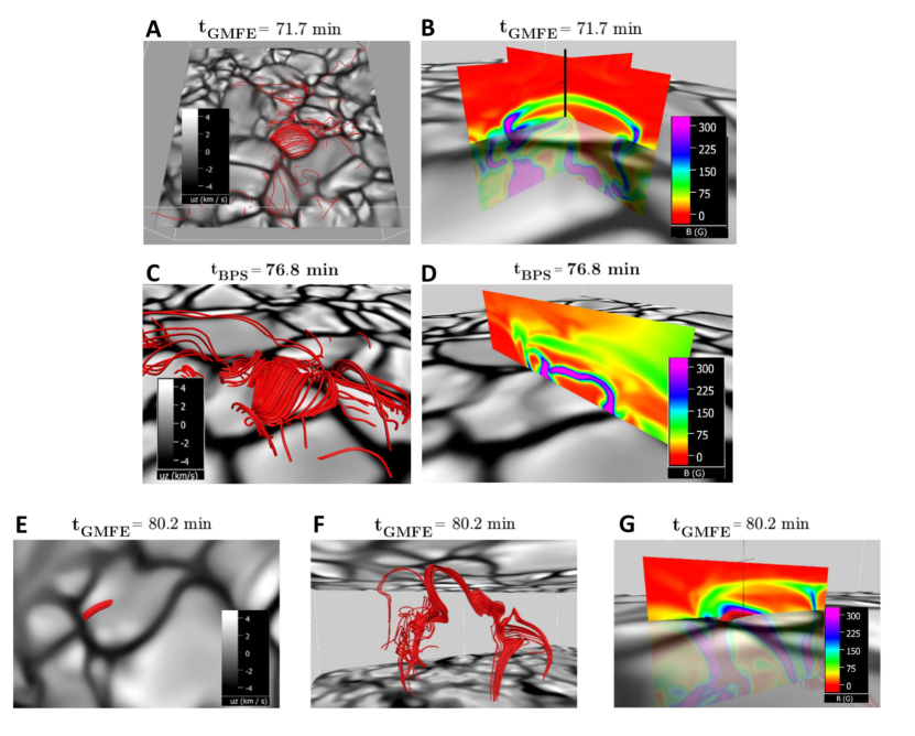
Figure 1: Panels A-D: magnetic sheet-like configurations revealed through fieldline tracing. A: sheet in the GMFE model, with (B) two orthogonal field-strength maps showing vertical cross sections. (See also the accompanying animation). C: sheet in the BPS, with (D) an accompanying field strength map. Panels E-G: emergence of an individual flux tube (perspective from above and below, respectively), with (G) corresponding $B$ map. Grayscale maps: ${u_{z}}$ at $z=0$; panel F also shows ${u_{z}}$ at $2.5$ Mm depth. The time tag indicates the simulation used. (An animation of this figure is available.)

2 Method

The two magnetoconvection simulations used in this Letter were calculated with the Bifrost radiation-MHD code (Gudiksen et al., 2011). In both, the zero of the vertical coordinate ($z$) is set at the average height of the ${\tau_{500}}=1$ corrugated surface and the bottom of the box is close to $z=-2.5$ Mm. The first one (hereafter the GMFE model) is a global magnetic flux emergence model with a domain of $10~{}\times~{}10~{}\times~{}15$ Mm³ in the $(x,y,z)$ directions. The grid resolution is $19.5$ km horizontally and better than $22$ km vertically for $z<2$ Mm. A simple, straight, twisted horizontal magnetic tube with $B_{\rm axis}=7.85$ kG and total flux $\Phi=10^{19}$ Mx is injected through the bottom boundary for $13$ solar minutes until $t=24$ minute following the prescription of Martínez-Sykora et al. (2008). The convective flows drag part of the injected field toward the surface; major arrival of flux at the surface occurs around $t=60-70$ minutes. The events described here occur in the subsequent $85$ minutes. The second model is the Bifrost public simulation of an enhanced network region (hereafter the BPS model) described in detail by Carlsson et al. (2016). Its domain is $24~{}\times 24~{}\times~{}16.9$ Mm³; the resolution is $48$ km horizontally and better than $19$ km vertically for $z<5$ Mm, with snapshots available for $26.5$ solar minutes. Instead of injecting magnetic flux, a global bipolar potential field was implanted throughout the box at $t=29$ minutes, allowed to be distorted by the convection in the near-surface and subphotospheric layers, and then relax. In the time interval studied here, both models had reached statistically stationary values of density, temperature, and internal energy throughout the convection zone.

Concerning the surface field, in the GMFE model at the time of maximum vertical unsigned flux, ${B_{\rm rms}}=72$ G and $<B>=29$ G on the ${\tau_{500}}=1$ surface. A degraded data set (rebinned and point-spread function (PSF)-convolved to approximate the Hinode resolution) yields similar values. This is within a factor $2$ of the observationally based quiet-Sun values of Khomenko et al. (2005) or Beck et al. (2017). On the other hand, in the BPS, $<B>=48$ G in the photosphere.

3 Photospheric flux emergence

In order to discern flux emergence patterns in photospheric levels, we calculate the magnetic linkage between photospheric elements (Section 3.1) and Stokes polarization maps for synthetic $\textrm{Fe}\,\textsc{i}\ 630.25$ nm spectra (Section 3.2).

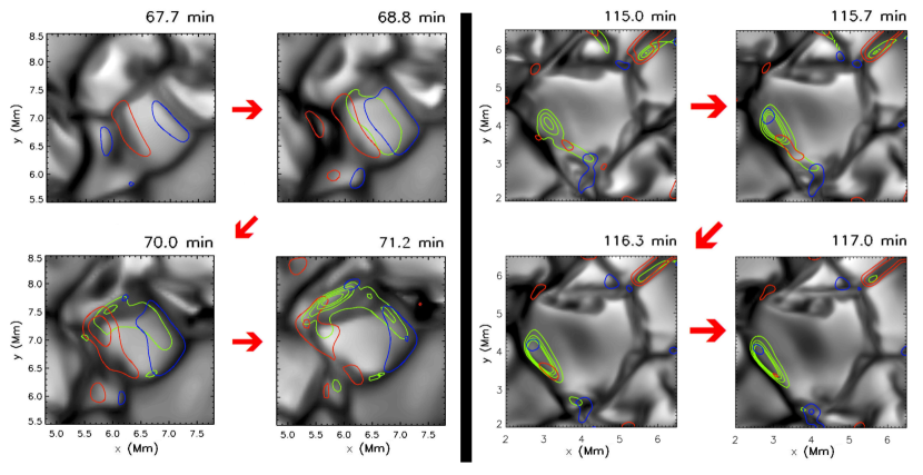
Figure 2: Time evolution of the polarization isocontours (red and blue: ${V_{int}}$; green: ${L_{int}}$) for a sheet (left) and a mini-tube (right) structure. Background grayscale map: the continuum intensity. Left half: the granule-filling sheet of Panels A-B of Figure 1. Right half: a tube emergence event. (An animation of this figure is available.)

3.1 3D magnetic linkage

Sheets: tracing magnetic field lines in the slab $0<z<270$ km in the GMFE model from random seeds biased toward strong B, we see episodes where a granule becomes covered by an ordered magnetic-field blanket: one of them is illustrated in Figure 1 (Panel A). The accompanying animation shows the global picture. Panel B shows field strength maps on orthogonal vertical planes that cut the blanket: the sheet is indeed a dome-like structure of predominantly horizontal field at $z\sim 300$ km with $B\sim 100$ G. A sheet formation instance in the BPS simulation is shown on panels C and D: field lines and (a single) field strength color map indicate the presence of a sheet appearing in a growing granule. Along the period studied in the GMFE model, we count at least six clear episodes of magnetic sheet formation, i.e., of orderly blanket-like magnetic field structures overarching a whole granule. The sheets reach basically only up to a few to several hundred km above the photosphere, hence like standard rising plasma elements in granules (see Cheung et al., 2007b; Tortosa-Andreu & Moreno-Insertis, 2009). In most cases the magnetic sheet, after rising a few hundred km above $z=0$, just disappears as a coherent structure and does not outlive the granule that it covers; in at least one case, however, the flux continues rising to the chromosphere. In the BPS run, we have identified three sheet formation episodes.

Tubes: to try to spot emerging-tube cases inside granules via fieldline linkage, we restrict the seeds for the tracing to emerging regions exclusively (${u_{z}}>0$). An instance of emerging micro flux tube in the GMFE model is shown in Figure 1 (bottom row): viewed from above the surface (panel E), a tube is seen emerging within a granule. Viewed from below (panel F), a tube-like concentration is seen down to depths of at least several $100$ km. Using a field-strength map on a vertical plane (panel G), we ascertain that the tube is not part of a sheet, and that it just grazes the photosphere, where it has $B\sim 300$ G: the tube does not rise beyond the first $100$ km above the photosphere.

The identification of rising tubes via fieldline linkage is often laborious. As an alternative, we next follow a semi-observational approach using synthetic Stokes profiles.

                      

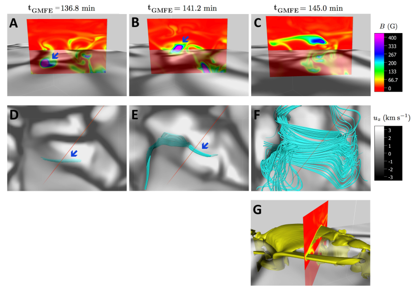
Figure 3: Formation of a magnetic sheet in a nascent granule. Upper row: vertical map for $B$. Middle row: top view with field lines that illustrate the formation of the sheet. Bottom panel: the $B=100$ G isosurface. The semi-transparent grayscale maps correspond to ${u_{z}}(z=0)$. The time for each column is given at the top.

3.2 Spectropolarimetric synthesis

For comparison with the observations, we have calculated synthetic spectra for the $\textrm{Fe}\,\textsc{i}\ 630.25$ nm line emitted by the plasma along vertical columns in the GMFE model. Using the Nicole code (Socas-Navarro et al., 2015), the four Stokes parameters, $I$, $Q$, $U$, $V$, were determined assuming LTE and with spectral resolution of $3.3$ mÅ. Following standard procedures (e.g., Lites et al., 2008; Sainz Dalda et al., 2012), for each vertical column we define the total degree of circular and linear polarization as

$$\displaystyle{V_{int}}=\frac{1}{\lambda_{r}-\lambda_{b}}\,\int_{\lambda_{b}}^{\lambda_{r}}\frac{|V(\lambda)|}{{I_{cont}}}\,d\lambda\hfill\hbox to48.36958pt{\hfill}$$ (1)

and (2)

$$\displaystyle{L_{int}}=\frac{1}{\lambda_{r}-\lambda_{b}}\,\int_{\lambda_{b}}^{\lambda_{r}}\frac{\sqrt{Q^{2}(\lambda)+U^{2}(\lambda)}}{{I_{cont}}}\,d\lambda\;,\hfill$$

respectively, with $\lambda_{b}=630.225$ nm, $\lambda_{r}=630.272$ nm, and ${I_{cont}}$ the continuum intensity near the spectral line averaged for each snapshot. A sign is given to ${V_{int}}$ according to that of the extremum of $V$ blueward of the line center. ${V_{int}}$ and ${L_{int}}$ provide a measure for vertical and transverse magnetic field strength, respectively, in the line-forming heights (${\tau_{500}}\sim 0.01$ for this line, see Balthasar 1988; Ruiz Cobo & del Toro Iniesta 1994). With ${V_{int}}$ and ${L_{int}}$ we construct polarization maps and try to detect the appearance of coherent magnetic structures in the photosphere.

Figure 2 (left half) shows a time sequence of isoline maps for ${V_{int}}$ (red=positive, blue=negative, two contours each for $|{V_{int}}|=6\times 10^{-3}$ and $3\times 10^{-3}$) and ${L_{int}}$ (green, four contours equally spaced up to ${L_{int}}=4\times 10^{-3}$) along $3.5$ minutes on the background of a grayscale map of the total intensity ${I_{cont}}$ for the magnetic sheet shown in the top left panel of Figure 1. The circular and linear polarization signals appear basically simultaneously; the latter seem to fill the granule shortly after first identification, as if a magnetic sheet had covered it. In the accompanying animation, other sheet cases can be identified; they seem to appear quasi-simultaneously with the granule with a surface-filling nature.

Additionally, there are many instances in which the Stokes contours seem to indicate that a coherent, tiny flux loop is emerging through the photosphere. A clear case from the GMFE model is illustrated in Figure 2 (right half): a linear polarization pattern appears in the granule interior, which $40$ s later is flanked by two circular polarization patches (top panels). Those patches split apart in time, the structure reaches the intergranular lane (bottom panels), and about a minute later it disappears.

We have found at least $19$ tube-like subgranular emergence events in the Stokes maps in the GMFE model (see animation for Figure 2). Although suggestive of an emerging loop or sheet, the indications gained through the Stokes polarization maps should be confirmed through 3D visualization including deeper levels, as done below.

4 Subphotospheric evolution

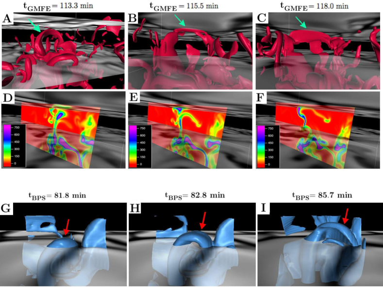
Figure 4: Panels A-F: time evolution of an arch-like field concentration that produces the Stokes contours of Figure 2 (right half). Top row: $B=500$-G isosurfaces. The two grayscale maps correspond to ${u_{z}}$ at, respectively, $z=0$ (solid) and $z=-1.5$ Mm (semi-transparent). Middle row: $B$-maps (in Gauss) on vertical planes cutting across the magnetic arches. Panels G-I: a subgranular flux-tube emergence event from the BPS.

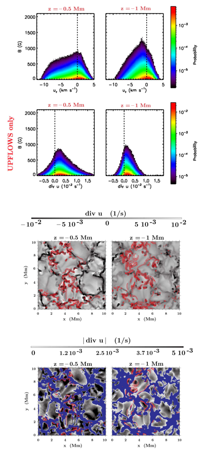
Figure 5: JPDFs of $B$ vs. ${u_{z}}$ (top row), and of $B$ vs. ${\bf div}\,{\bf u}$ (second row, for upflowing plasma alone), calculated from the GMFE model between $t=80$ - $140$ minutes with $10$ s cadence. Pixels with $B<20$ G are excluded. Lower half: grayscale maps of ${\bf div}\,{\bf u}$ (3rd row) and $|{\bf div}\,{\bf u}|$ (4th row) both at $t=101.3$ minutes and with $B=[140,280,560]$ G isocontours superimposed. A blue mask covers the downflows in the 4th row.

4.1 The formation of a magnetic sheet

The magnetic sheets may be naturally associated with the formation of a granule in a subphotospheric magnetized region: the magnetized plasma will be raised and expand sideways as the granule develops; a blanket of ordered, horizontal field may result near the photosphere.

Figure 3 corresponds to three instants in the development of such a sheet. A tube-like magnetic concentration had formed a few hundred km below the photosphere: at some point it is lifted by a nascent granule and leads to the formation of a sheet. The upper panel row contains a side view with a vertical color map of $B$. The middle row contains a top view of the same snapshots: the plane of the $B$ map is now seen edge-on. Field lines have been traced from seeds in small boxes containing the relevant field concentrations in the $B$-maps. Initially (left column), the subphotospheric magnetic tube was rising toward the photosphere, but it gets caught in a downdraft and is prevented from rising to $z=0$. The magnetic concentration (blue arrow) is located at $z\approx-0.43$ Mm and has a diameter of a few hundred km. Some four minutes later (central column) the tube has wandered off the downdraft and is part of an incipient granule, which pulls it up through the surface. In the later instants (rightmost panels), the magnetized plasma is lifted to heights a few hundred km above the photosphere. In doing so, it is stretched sideways such that a magnetic sheet is created: in panel C the tube is still recognizable on the right, but a roughly horizontal magnetic sheet with $B\sim 100$ G at $z\sim 200$–$400$ km is seen to cover a granular-sized region. The corresponding field lines (panel F) constitute a sort of blanket; that shape is also clear from the corresponding $B=100$ G isosurface (panel G).

4.2 The subsurface evolution of a tube-like feature

Is the bipolar feature appearing in a granule in Figure 2 (right) really caused by a magnetic tube rising below the surface? Figure 4 contains (top row) $B=500$ G isosurfaces below the photosphere in a region that includes the domain of Figure 2 (right half). In panel A, a prominent arch-like feature (marked with an arrow) is seen right below the area shown in Figure 2, and is about to cause a bipolar feature at the surface. Checking back in time, one can trace this arched concentration to at least $13$ minutes earlier, when it is seen around $1.5$ Mm depth, rising at the fringes of an upflowing convective plume. Panel B contains a blow-up of the central arch: its apex has already reached the photosphere and is producing the bipolar feature of Figure 2. Panel C shows the magnetic concentration at the photosphere being swallowed by the intergranular lane. The central panel row shows $B$-maps on vertical planes that cut across the rising magnetic structure, confirming that the $B$-isosurfaces really correspond to magnetic concentrations. The bottom row (panels G-I) contains $B=150$ G isosurfaces from a subgranular tube-emergence event in the BPS; an arched region is seen to emerge in a transverse direction to the granule boundary; it is then pushed sideways toward the intergranule and finally swallowed by the latter. Both in the GMFE model and in the BPS, we have also tested the flux-tube nature of the magnetic arches: field lines traced from within the isosurfaces stay within them in the region occupied by the arch.

There are two important differences between the formation of sheets and tubes. The tube-like features here had a concentrated, tube-like shape in deep levels and were rising as part of a developed granule, whereas the structure in Section 4.1 was picked up at shallow levels by an incipient granule. The tube cases in the present section, although stretched sideways when rising above the surface, did not lead to a granule-covering magnetic sheet.

4.3 The subphotospheric origin of the emerging flux concentrations

To locate the origin of the rising concentrated magnetic structures detected in the experiments, we here use the GMFE model to put together different pieces of evidence.

(a) There is an important fraction of non-weakly magnetized plasma elements located in upflows: the $B$-${u_{z}}$ JPDFs of Figure 5 (top row) show that the peak probability for the strong-field elements (say, $B\gtrsim 300$ G) at $1$ Mm depth are in the downflow regions, as expected from magnetoconvection theory (Pietarila Graham et al., 2010, e.g.), but, also, that a significant fraction of the cases with $B$ up to several hundred Gauss is located in upflows (which also applies to the $z=-0.5$ Mm JPDF).

(b) Many of those structures can survive for tens of minutes retaining high values of the field strength. From the $B$-${\bf div}\,{\bf u}$ JPDFs in the upflows (second row), we see that the majority of strongly magnetized elements (say, $B\gtrsim 300$ G) have very low (or negative) expansion rates, typically ${\bf div}\,{\bf u}\lesssim 3\times 10^{-3}$ s^-1. If expanding isotropically at that rate, $B$ would decrease by a factor $10$ in a few tens of minutes. That is, therefore, also the typical minimum survival time that we expect for the strong magnetic fields in those levels.

(c) The strongly magnetized volumes found in upflows are generally located in the neighborhood of downflows. The third and fourth panel rows contain grayscale maps of ${\bf div}\,{\bf u}$ at $z=0.5$ and $1$ Mm with isocontours for $B=140,280,$ and $560$ G superimposed. We see that the strong fields alineated with the downflowing regions (third row); however, blocking the downflows with a blue mask (fourth row), we see that part of the strong fields are moving upwards.

We conclude that most of the stronger field concentrations are created in or near the downflowing regions. With lifetimes and velocities as deduced from the JPDFs, we estimate that the magnetic arches can go across, say, $1$ Mm. Because additionally the upflow domains expel the plasma toward their boundaries well before reaching the surface (see Stein, 2012), we see that a concentrated magnetic structure is likely to remain in the neighborhood of the downflow where it was created for its entire life. The majority of flux tube examples studied in our simulations do not live longer than $30$ minutes in upflow regions continuously; those formed below $z=-1$ Mm are unlikely to emerge all the way to the photosphere.

5 Discussion

In this Letter, we have identified two types of small-scale emerging magnetic structures in the solar photosphere: sheets that at maximum development cover the granular surface (or almost do), and small magnetic tubes surfacing within the granular cell. To do this, we have combined statistical and visualization tools to (a) discern coherent, emerging magnetic structures on subgranular scales in 3D numerical models of quiet-Sun magnetoconvection and (b) investigate their origin, nature, and time evolution. A first tally yields $19$ rising-flux tube and six magnetic sheet events in the GMFE model; in the BPS we count at least three flux-sheet and ten flux-tube emergence episodes. A rough frequency of appearance of these events in the models is therefore between $1$ and $3$ day^-1 Mm^-2 for tube-like events, and between $0.3$ and $1$ day^-1 Mm^-2 for sheet-like ones. The detection of these events in both the GMFE model and the BPS is significant, as the latter is not a global flux emergence simulation.

We conclude that granule-covering flux sheets and tiny, subgranular emerging tubes are different categories of emerging magnetic structures. The magnetic sheets seem to be created when a granule is formed in a location traversed by a small subphotospheric magnetic tube: in the early stages, the granules have a small size and the tube may fill an important fraction of the nascent granule’s area at the surface. The subsequent sideways stretching and vertical compression of the magnetized plasma volume when reaching, say, a few hundred km above the surface leads to a flattened magnetic structure that covers most of the granule. Instead, the tubes appear also in later stages of development of the granules and do not cover their whole surface. They seem to retain a distinctive flux tube shape from deep levels of the convective cell (e.g., from $z=1.5$ Mm) while rising in the cell’s updraft. Based in part on a statistical study we have concluded that, in the deep levels, the rising concentrated tubes are preferentially located in the neighborhood of the downflows and have low expansion rates: some can rise across distances of order $1$ Mm without being weakened by expansion nor being brought back down toward deeper levels.

On the observational side, there have been clear hints for the emergence of small arch-like tubes within granules for about 10 years now (as detailed in the Introduction), whereas it is only recently that Centeno et al. (2017) may have detected granule-covering flux sheets. On our side, we have carried out a preliminary forward-modeling exercise through the a posteriori calculation of Stokes parameters for the $\textrm{Fe}\,\textsc{i}\ 630.25$ nm line for the GMFE model simulation (Section 3.2). We could draw maps of the vertical and horizontal polarization levels and locate abundant episodes that bear clear similarities to the observations.

A full report, more detailed forward-modeling, and inclusion of further numerical simulations are left for a future publication.

References

- Balthasar (1988) Balthasar, H. 1988, A&AS, 72, 473
- Beck et al. (2017) Beck, C., Fabbian, D., Rezaei, R., & Puschmann, K. G. 2017, ApJ, 842, 37
- Carlsson et al. (2016) Carlsson, M., Hansteen, V. H., Gudiksen, B. V., Leenaarts, J., & De Pontieu, B. 2016, A&A, 585, A4
- Centeno et al. (2007) Centeno, R., Socas-Navarro, H., Lites, B.,et al. 2007, ApJ, 666, L137
- Centeno et al. (2017) Centeno, R., Blanco Rodríguez, J., Del Toro Iniesta, J.C., et al. 2017, ApJS, 229, 3
- Cheung et al. (2010) Cheung, M. C. M., Rempel, M., Title, A. M., & Schüssler, M. 2010, ApJ, 720, 233
- Cheung et al. (2007a) Cheung, M. C. M., Schüssler, M., & Moreno-Insertis, F. 2007a, A&A, 467, 703
- Cheung et al. (2007b) —. 2007b, A&A, 461, 1163
- Cheung et al. (2008) Cheung, M. C. M., Schüssler, M., Tarbell, T. D., & Title, A. M. 2008, ApJ, 687, 1373
- Clyne et al. (2007) Clyne, J., Mininni, P., Norton, A., & Rast, M. 2007, New Journal of Physics, 9, 301
- de la Cruz Rodríguez et al. (2015) de la Cruz Rodríguez, J., Hansteen, V., Bellot-Rubio, L., & Ortiz, A. 2015, ApJ, 810, 145
- Gömöry et al. (2010) Gömöry, P., Beck, C., Balthasar, H., et al. 2010, A&A, 511, A14+
- Gošić et al. (2016) Gošić, M., Bellot Rubio, L. R., del Toro Iniesta, J. C., Orozco Suárez, D., & Katsukawa, Y. 2016, ApJ, 820, 35
- Gošić et al. (2014) Gošić, M., Bellot Rubio, L. R., Orozco Suárez, D., Katsukawa, Y., & del Toro Iniesta, J. C. 2014, ApJ, 797, 49
- Gudiksen et al. (2011) Gudiksen, B. V., Carlsson, M., Hansteen, V. H., Hayek, W., Leenaarts, J., & Martínez-Sykora, J. 2011, A&A, 531, A154
- Guglielmino et al. (2012) Guglielmino, S. L., Martínez Pillet, V., Bonet, J.A. et al. 2012, ApJ, 745, 160
- Khomenko et al. (2005) Khomenko, E. V., Martínez González, M. J., Collados, M., et al. 2005, A&A, 436, L27
- Lites et al. (2008) Lites, B. W., Kubo, M., Socas-Navarro, H. et al. 2008, ApJ, 672, 1237
- Martínez González & Bellot Rubio (2009) Martínez González, M. J., & Bellot Rubio, L. R. 2009, ApJ, 700, 1391
- Martínez-Sykora et al. (2008) Martínez-Sykora, J., Hansteen, V., & Carlsson, M. 2008, ApJ, 679, 871
- Martínez-Sykora et al. (2009) —. 2009, ApJ, 702, 129
- Nordlund et al. (2009) Nordlund, Å., Stein, R. F., & Asplund, M. 2009, Living Reviews in Solar Physics, 6, 2
- Ortiz et al. (2014) Ortiz, A., Bellot Rubio, L. R., Hansteen, V. H., de la Cruz Rodríguez, J., & Rouppe van der Voort, L. 2014, ApJ, 781, 126
- Ortiz et al. (2016) Ortiz, A., Hansteen, V. H., Bellot Rubio, L. R., de la Cruz Rodríguez, J., De Pontieu, B., Carlsson, M., & Rouppe van der Voort, L. 2016, ApJ, 825, 93
- Palacios et al. (2012) Palacios, J., Blanco Rodríguez, J., Vargas Domínguez, S., et al. 2012, A&A, 537, A21
- Pietarila Graham et al. (2010) Pietarila Graham, J., Cameron, R., & Schüssler, M. 2010, ApJ, 714, 1606
- Ruiz Cobo & del Toro Iniesta (1994) Ruiz Cobo, B., & del Toro Iniesta, J. C. 1994, A&A, 283, 129
- Sainz Dalda et al. (2012) Sainz Dalda, A., Martínez-Sykora, J., Bellot Rubio, L., & Title, A. 2012, ApJ, 748, 38
- Socas-Navarro et al. (2015) Socas-Navarro, H., de la Cruz Rodríguez, J., Asensio Ramos, A., Trujillo Bueno, J., & Ruiz Cobo, B. 2015, A&A, 577, A7
- Stein (2012) Stein, R. F. 2012, Living Reviews in Solar Physics, 9, 4
- Stein & Nordlund (2006) Stein, R. F., & Nordlund, Å. 2006, ApJ, 642, 1246
- Tortosa-Andreu & Moreno-Insertis (2009) Tortosa-Andreu, A., & Moreno-Insertis, F. 2009, A&A, 507, 949