Vertical drafts and mixing in stratified turbulence: sharp transition with Froude number

Abstract

We investigate the large-scale intermittency of vertical velocity and temperature, and the mixing properties of stably stratified turbulent flows using both Lagrangian and Eulerian fields from direct numerical simulations, in a parameter space relevant for the atmosphere and the oceans. Over a range of Froude numbers of geophysical interest ($\approx 0.05-0.3$) we observe very large fluctuations of the vertical components of the velocity and the potential temperature, localized in space and time, with a sharp transition leading to non-Gaussian wings of the probability distribution functions. This behavior is captured by a simple model representing the competition between gravity waves on a fast time-scale and nonlinear steepening on a slower time-scale. The existence of a resonant regime characterized by enhanced large-scale intermittency, as understood within the framework of the proposed model, is then linked to the emergence of structures in the velocity and potential temperature fields, localized overturning and mixing. Finally, in the same regime we observe a linear scaling of the mixing efficiency with the Froude number and an increase of its value of roughly one order of magnitude.

I Introduction

Intermittency is a hallmark of fully developed turbulence in fluids. Contrary to the predictions of the Kolmogorov’s original theory K41 , both experiments and numerical simulations show that dissipation exhibits intense (intermittent) fluctuations, localized in space and time, giving rise to a characteristic behavior of quiescence interrupted by local bursts of high amplitude kolmogorov_62 ; frisch_80 . This phenomenon, known as small-scale intermittency, is widely observed in the atmosphere fritts_13b , where it can explain the formation of rain droplets falkovich_07 ; Bodenschatz , and in the ocean in the form of highly concentrated and sporadic dissipation klymak_08 ; pearson_18 . Small-scale intermittency is often characterized by the strong deviations from Gaussian statistics of the probability distribution functions (PDF) of velocity and temperature gradients. Intermittency, however, is not only present at the smallest scales. In transitional pipe flows barkley_15 , in the problem of mixing of a passive scalar by a turbulent flow PSS91 , in the solar wind marino_12 , and for stratified flows as in the Earth’s atmosphere chau and in the oceans, non-stationary energetic bursts at scales comparable to that of the mean flow are also observed mahrt_89 ; dasaro_11 ; rorai_14 ; pearson_18 . The origin of this large-scale intermittency in stratified turbulence and the mechanisms by which it may affect overturning and mixing in geophysical flows are still unclear. In the present letter we characterize the vertical drafts occurring at a large scale, using direct numerical simulations (DNS) of stably stratified Boussinesq flows, varying the buoyancy frequency. The large scale intermittent behavior is studied here by direct integration of the Boussinesq equations, without any parametrization of the smaller scales and with periodic boundaries, contrary to what was done in previous work. In particular, we relate the wings of the PDFs of the vertical component of Lagrangian and Eulerian velocities and of the potential temperature, to large-scale bursts, which result from the interplay of gravity waves and turbulent motions in a range of Froude numbers relevant to geophysical flows. This is explained with the help of a simple one-dimensional (1D) model, which captures the extreme events rorai_14 and the sharp transition observed in our simulations between Gaussian and non-Gaussian PDFs. Finally we provide clear evidence of the connection between local overturning events and mixing in stratified flows $-$ characterized through the gradient Richardson number Rosenberg_15 , the mixing efficiency and the ratio of kinetic to potential energy $-$ with the emergence of large-scale intermittency and structures.

II Equations, parameters, and runs

The Boussinesq approximation assumes that the variations of density are small and depend linearly on temperature; they are neglected, except in the expression of the buoyancy force. The incompressible velocity field $\mathbf{u}$ ($\nabla\cdot\mathbf{u}=0$) and temperature, expressed in suitable units satisfy:

$$\partial_{t}\textbf{u}+(\textbf{u}\cdot\nabla)\textbf{u} = -\nabla p-N\theta\hat{z}+\textbf{F}+\nu\nabla^{2}\textbf{u}$$ (1)

$$\partial_{t}\theta+\textbf{u}\cdot\nabla\theta = Nw+\kappa\nabla^{2}\theta\,$$ (2)

where $\theta$ is a temperature fluctuation relative to the mean $\overline{\theta}$, $\nu$ is the kinematic viscosity, and $\kappa=\nu$ is the thermal diffusivity. The velocity field is written as $\textbf{u}=({\bf u}_{\perp},w)$ and the flows in this study are subject to a random isotropic mechanical forcing F (as also described in marino_14 ), applied in a wavenumber shell: $k_{F}=2\pi/L_{f}\in[2,3]$, the size of the periodic three-dimensional computational box being $L_{0}=2\pi$. Finally, $N=\left[-g\partial_{z}\overline{\theta}/\theta_{0}\right]^{1/2}$ is the Brunt-Väisälä frequency.

Id	1	2	3	4	5	6	7	8	9	10	11	12	13	14	15	16	17
$Re$ $(\times 10^{3})$	3.8	3.8	3.8	3.8	3.8	3.8	3.9	3.8	3.8	3.8	3.7	3.6	3.0	2.6	2.6	2.8	2.9
$Fr$	.015	.026	.030	.038	.044	.051	.068	.072	.076	.081	.098	.11	.16	.19	.28	.56	.93
$K_{\tilde{w}}$	3.11	3.17	3.07	3.06	3.17	3.41	7.40	9.50	10.44	9.39	8.86	5.63	3.87	3.53	3.30	2.95	3.00
$\ell_{Oz}$	.07	.014	.018	.024	.029	.037	.056	.061	.067	.076	.11	.14	.39	.65	1.25	3.66	8.00
$R_{B}$	.9	2.5	3.4	5.6	7.3	10.2	17.7	19.7	22.1	25.2	35.9	47.5	75.2	90.9	201	895	2560

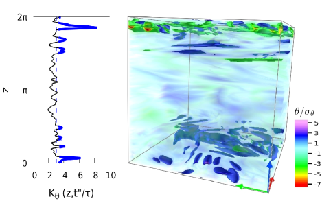
Figure 4: Variation with height of the kurtosis of the potential temperature ($\theta$), computed by plane for run 9 at fixed time $(t^{\prime\prime}/\tau$, relative maximum of $K_{w}(t/\tau)$, Fig.2$)$, together with the rendering of $\theta$ for the same run. A threshold is used to highlight with opaque colors the presence of hot and cold patches with temperature fluctuations larger than 3 standard deviations $(\sigma_{\theta})$, corresponding here to the planes with the largest values of the kurtosis.

Table 1: Table of the runs. Reynolds, Froude and buoyancy Reynolds numbers are respectively $Re$, $Fr$ and $R_{B}$; $\ell_{Oz}$ is the Ozmidov scale; $K_{\tilde{w}}$ is the kurtosis of the Lagrangian PDFs computed over the entire integration interval of the particles. Run 9 (boldface) has the highest $K_{\tilde{w}}$ and is used as a reference case for the visualizations in Figures 3 and 4.

We define the Reynolds and Froude numbers, the dimensionless parameters of the problem: $Re=UL/\nu,\ Fr=U/LN$, where $U,L$ are respectively the characteristic velocity and the integral scale of the fluid. The buoyancy Reynolds number, $R_{B}\equiv Re\,Fr^{2}=\Big{(}\ell_{Oz}/\eta\Big{)}^{4/3}$, where $\ell_{Oz}\equiv(\varepsilon_{V}/N^{3})^{1/2}$ and $\eta\equiv(\varepsilon_{V}/\nu^{3})^{-1/4}$ are the Ozmidov and Kolmogorov dissipation lengths, and $\varepsilon_{V}\equiv\nu\langle(\nabla\mathbf{u})^{2}\rangle$ is the kinetic energy dissipation rate. $R_{B}$ measures the relative strength of buoyancy and dissipation: for $R_{B}=1$, the Ozmidov scale at which dispersive and nonlinear effects balance is at the Kolmogorov scale. To solve these equations numerically we use the Geophysical High-Order Suite for Turbulence (GHOST) code, a versatile pseudo-spectral framework parallelized with a hybrid MPI/OpenMP method hybrid_11 . All computations are performed on isotropic grids of $512^{3}$ points, altogether for of the order of 40 $\tau$, where $\tau=L/U$ is the turn-over time. Together with the Eulerian velocity and temperature field, we determined also the trajectories of tracer particles in the flow, whose positions ${\bf X}({\bf X}_{0},t)$ satisfy $\partial_{t}{\bf X}({\bf X}_{0},t)={\bf u}({\bf X}({\bf X}_{0},t),t)$ (with $\mathbf{X}(\mathbf{X}_{0},0)=\mathbf{X}_{0}$). We followed $n\approx 1.5\cdot 10^{6}$ particle trajectories, initially uniformly distributed in space. They are injected randomly after turbulence becomes fully developed, i.e., after the dissipation in the flow has reached its maximum (see Fig. 2), and their trajectories are determined for a duration of 6 to 10 turnover times. Lagrangian temporal statistics are always collected throughout the entire time of integration. To characterize the statistical distribution of a fluctuating variable, we introduce the dimensionless fourth-order moment (kurtosis), defined as:

$$K_{\alpha}=\langle\alpha^{4}\rangle/\langle\alpha^{2}\rangle^{2}\\$$ (3)

where $\alpha$ is the generic field and averages can be taken over the entire box, horizontal planes, time, or over ensembles of particles as specified below. The Gaussian reference value of the kurtosis is equal to 3.

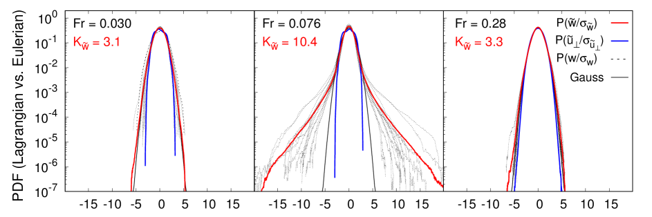
Figure 1: PDFs of the Lagrangian vertical velocity $\tilde{w}$ (solid line, red), Lagrangian horizontal velocity $\tilde{u}_{\perp}$ (solid line, blue) and instantaneous Eulerian vertical velocity $w$ at several times (all dashed lines, black), for runs 3 (left), 9 (middle) and 15 (right). All quantities are normalized by their dispersion. A Gaussian PDF is indicated as reference in each panel (solid line, black).

The Reynolds number varies roughly by $35\%$ throughout the parametric study, from $\approx 2600$ to $\approx 3900$. All the runs have been initialized with zero potential temperature and a random velocity field with energy distributed on spherical shells centered on the wavenumber $k_{0}=2\pi/L_{0}$ in the range $k_{0}=[2,3]$.

III Large scale intermittency in stratified flows

As a result of the stratification, the Lagrangian particles mostly wander around in horizontal planes, with sharp vertical excursions which leave a signature in the PDFs of $w$ and $\tilde{w}$, respectively the vertical component of the Eulerian velocity field and the vertical velocities of the Lagrangian particles. Figure 1 gives both the instantaneous PDFs of $w$, each corresponding to a dotted curve (computed every 1000 time-steps of the DNS, within the domain of integration of the particles), and PDFs of the Lagrangian particles velocity $\tilde{w}$ (solid red curves), for three different Froude numbers. In all plots, the Lagrangian PDFs appear, up to statistical errors, as the time average of the instantaneous Eulerian PDFs. In the case shown in the middle panel ($Fr=0.076$), the wings for high values of $w$ and $\tilde{w}$ are significantly broader than the Gaussian wings, with a kurtosis of the Lagrangian particles velocity $K_{\tilde{w}}\approx 10.44$. This is the signature of the occurrence of extreme events at some time in the evolution of the flow, in some regions of the spatial domain. The departures from the Gaussian behavior are very weak for the cases with smaller and larger Froude number displayed in the lateral panels ($Fr=0.03$ and $Fr=0.28$, respectively left and right), with the kurtosis becoming $K_{\tilde{w}}\approx 3$ for the smallest and highest $Fr$ considered in this parametric exploration (see Table 1).

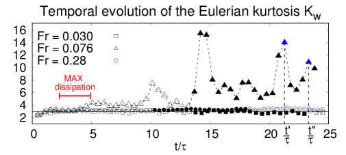
Figure 2: Kurtosis of the Eulerian vertical velocity $(w)$ as a function of time for runs 3,9 and 15. Each point is the statistical moment (eq. 3) of the corresponding instantaneous PDFs showed in Fig.1 (dashed lines). Solid symbols identify the periods of integration of the Lagrangian particles, injected systematically after the peak of the dissipation, here indicated with a red segment for the runs displayed. Points in blue identify the relative maxima at which the Eulerian fields of run 9 $(Fr=0.076)$ are rendered in Figures 3 and 4.

Fig. 1 also shows the PDFs of the horizontal Lagrangian components of the velocity field $\tilde{u}_{\perp}$ (solid blue line) that is markedly below the Gaussian distribution, in all 17 runs. For some of the stratified flows under study, the instantaneous PDFs of the Eulerian vertical velocity $w$ vary strongly over time, as it is for run 9 in Fig. 1 (dotted lines, middle panel). This time-dependence leads to strong fluctuations of the corresponding Eulerian PDFs’ kurtosis, $K_{w}$, shown in Fig. 2 ($Fr=0.076$). The kurtosis of the Lagrangian PDFs, $K_{\tilde{w}}$, resulting from global spatio-temporal statistics of $1.5\cdot 10^{6}$ particles’ vertical velocities (over the entire integration time) is plotted in Fig. 5 against the Froude number for the runs in Table 1. It is noteworthy that the curve $K_{\tilde{w}}(Fr)$ is characterized by a non-monotonic behavior, showing a rapid increase and then decrease of the Lagrangian kurtosis in a sharp range between $Fr\approx 0.05$ and $\approx 0.3$, with a peak centered around $Fr\approx 0.076$. The kurtosis of temperature fluctuations (not shown) also deviates from 3 in the same range of parameters. This result provides clear evidence that stably stratified turbulent flows are characterized by large scale intermittency and strong vertical drafts in a well defined regime of stratification. It is also worth to point out that for all the runs outside the range $0.05<Fr<0.3$ no large-scale intermittency is detected from Lagrangian and Eulerian statistics and the kurtosis of the instantaneous Eulerian PDFs does not fluctuate and is constantly close to the Gaussian reference value ($K_{w}\approx 3$); this is illustrated in Figures 1 and 2 for the runs with $Fr=0.03$ and $=0.28$. One last important remark is that all the runs in the intermittent regime identified here have buoyancy Reynolds number $10<R_{B}<10^{2}$, whereas values of the Lagrangian kurtosis $K_{\tilde{w}}$ compatible with the Gaussian case are found for runs with $R_{B}\sim 1$ as well as $R_{B}\sim 10^{3}$ (Table 1). To better understand the origin of the strong updrafts and downdrafts in the vertical velocity, and their variation with $Fr$, we now introduce a simple model.

IV A model for the vertical drafts

It was found in rorai_14 that the intermittent behavior observed in a stratified fluid can be explained by a 1D model for the vertical velocity and the temperature based on vieillefosse_84 ; Li . In this model, the strong and fast events occur because of an amplification in the formation of vertical negative velocity gradients resulting from the interplay between the time scales of the waves and the nonlinearity. We generalize here this model adding both forcing and dissipation, in order to achieve a steady state and to control the growth of $w$. To this end we reduce Eqs. (1,2) to the 1D case, dependent only on the $z$ coordinate, and with ${\bf u}_{\perp}=0$. We derive the equations with respect to $z$ using $\partial_{z}(\partial_{t}a+w\partial_{z}a)=d_{t}(\partial_{z}a)+(\partial_{z}w)\,(\partial_{z}a)$ (for any field $a$, and where $d_{t}$ is the Lagrangian derivative in the vertical direction), and finally we convert spatial derivatives to increments by assuming fields are smooth on an arbitrary scale $\ell_{z}$, and thus $\delta a\approx\partial_{z}a\,\ell_{z}$. The resulting model has the same overall structure as the Boussinesq model, Eqs.(1,2), with viscous damping and mechanical forcing finally re-introduced in an empirical way:

$$\frac{d\delta w}{dt} = -\frac{\delta w^{2}}{\ell_{z}}-N\delta\theta-\nu\frac{\delta w}{\ell_{z}^{2}}+f$$ (4)

$$\frac{d\delta\theta}{dt} = -\frac{\delta w\delta\theta}{\ell_{z}}+N\delta w-\kappa\frac{\delta\theta}{\ell_{z}^{2}}\$$ (5)

For a fixed value of $\ell_{z}$ and for high enough $N$, waves prevail over turbulence, whereas for small $N$, turbulence prevails over waves. At intermediate values, a different behavior occurs, with a rapid increase of negative velocity field increments rorai_14 . This model can be seen as a 1D approximation to Lagrangian trajectories in a stratified flow, and at fixed $N$ with only one free parameter, the length scale $\ell_{z}$ representing the dominant gradients. The model was integrated using $N$, $\nu$ and $\kappa$ from the simulations (see Table 1), and for each case we ran an ensemble of 20 realizations (or Lagrangian particles) up to $t=20$, using a white-noise random forcing $f$ with frequencies between $N/8$ and $N$ to mimic the flat Lagrangian spectrum of the vertical velocity observed in stably stratified turbulence, the so-called Garrett-Munk spectrum ivey_08 . The amplitude of $f$ is the only tunable parameter that is not taken directly from the DNS and it was fixed to lead to finite amplitude solutions even in the weakly stratified cases (i.e. for moderate $N$). We adjusted the free parameter $\ell_{z}$ by assuming that the extreme events are the result of local shear instabilities or overturning (see Fig. 3, right), and thus the vertical scale at which these events take place can be expected to be proportional to the Ozmidov scale in each run, $\ell_{z}=\alpha\ell_{Oz}$ (note this scale also separates the boundary between wave- and eddy-dominated scales). In the following we use $\alpha=4$ which gives the best quantitative agreement with the DNS, but any choice for $\alpha$ of order unity gives the same qualitative results. Other choices for $\ell_{z}$, such as $\ell_{z}=L_{B}=2\pi U/N$ do not give results compatible with the DNS, which can be expected since, at the buoyancy scale $L_{B}$, the vertical Froude number is unity, and thus the behavior of the model becomes independent of $Fr$. Figure 5 (top) shows the kurtosis $K_{\tilde{w}}$ of the Lagrangian vertical velocities for all the DNS runs of this parametric study, together with the kurtosis of the Lagrangian field $\delta w$ generated by the 1D model initialized with the corresponding DNS parameters (red line). Each run is characterized by a different Froude number in a range of values spanning over one order of magnitude, from $\approx 0.01$ to $\approx 1$ (see Table 1). Note the behavior of both kurtoses confirms the results in Fig. 1: for intermediate values of $Fr$ the vertical velocity becomes very intermittent with values of the Lagrangian kurtosis $K_{\tilde{w}}$ larger than $10$. Considering its simplicity, the model reproduces qualitatively remarkably well the behavior found in the DNS. All quantities display a sharp peak for $Fr\approx 0.076$, with a decrease for higher Froude numbers. What is striking here is the sharpness of the peak in $Fr$ for all variables, as well as the asymmetry between the rising and descending phases of this transition. Such a sharp variation in $Fr\approx 0.076$ may be surprising; it evokes a wave resonance as occurs in critical layers when the flow velocity is equal to the wave phase speed, leading to the creation of jets. Indeed, similarly high values of kurtosis are found in atmospheric data in the upper boundary layer, and are interpreted as the signature of a global (large-scale) intermittency for a turbulence that is patchy and inhomogeneous mahrt_89 . In the model, both the peak and the asymmetry arise as the result of two competing effects: for large $Fr$ the nonlinear term dominates, amplifying negative velocity increments on a time scale of the turnover time; for small $Fr$ the linear term dominates, resulting in wave dynamics. But for intermediate values of $Fr$ the time scales of the two terms are similar, with an acceleration in the nonlinear amplification resulting from the slightly faster wave time scale. To the right and to the left of the peak, the nature of the dominant terms is different. We stress that the transition discussed here strongly differs from that observed when the buoyancy Reynolds number, $R_{B}$, is varied; this transition affects the small-scale flow properties (see, e.g., shih_05 ; ivey_08 ; pouquet_18 ).

V Structures, overturning and mixing

Thanks to a combined implementation of global spatio-temporal Lagrangian statistics and instantaneous Eulerian statistics we are able to show how the broad distributions observed in previous sections can in fact be linked to physical structures. Fig. 3 (left) provides the three-dimensional rendering of the vertical velocity $w$ for run 9, $Fr=0.076$, at the time $t^{\prime}/\tau$ when a local maximum of the instantaneous Eulerian kurtosis is attained based on the curve $K_{w}(t/\tau)$ in Fig.2. The side plot in Fig. 3 (left) shows the variation of the kurtosis obtained from integrations of the statistics in a single horizontal plane, plotted as a function of altitude, $K_{w}(z,t^{\prime}/\tau)$, which allow for the identification of the planes containing the strongest structures. On average in the flow, the variable is quasi-Gaussian, with $K_{w}(z,t^{\prime}/\tau)\sim 3$, except at some rare vertical positions, where the fluctuations of $w$ are much larger than the background fluctuations, with strong non-Gaussian properties. Similar conclusions can be drawn by analyzing the potential temperature $\theta$ in physical space, shown in Fig. 4. This bursty behavior at the large scales, in space and in time, is stronger in runs 7 to 12, resulting in the observed non-stationarity of the instantaneous Eulerian PDFs (Fig. 1, middle, and Fig. 2) and in the emergence of structures, Fig.3 (left) and Fig. 4. The intermittent behavior also affects the smallest scales of the flow: the dissipation and the gradient fields also have rare, intense structures embedded in the quiet flow (not shown, see rorai_14 ).

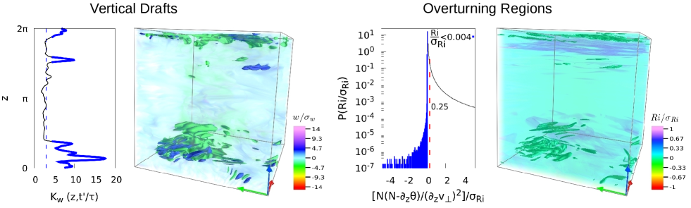
Figure 3: Left: Variation with height of the kurtosis of the Eulerian vertical velocity $(w)$, computed by plane for run 9 at fixed time $(t^{\prime}/\tau$, relative maximum of $K_{w}(t/\tau)$, Fig.2$)$, together with the rendering of $w$ for the same run. A threshold is used to highlight the presence of intense vertical drafts $(>3\sigma_{w})$ which appear as large-scale structures emerging in distinct planes that correspond to those with the largest values of the kurtosis. Right: PDF of the gradient Richardson number ($Ri=N(N-\partial_{z}\theta)/(\partial_{z}v_{\perp})^{2}$) normalized by its variance $(\sigma_{Ri})$, together with the rendering of its point-wise values where regions prone to develop overturning, with $Ri/\sigma_{Ri}<0.004$, are visualized using opaque colors.

Extreme updrafts and downdrafts affect the vertical transport. The product of the vertical temperature flux with the Brunt-Väisälä frequency $N$ is the so called buoyancy flux $B_{f}=N\left<w\theta\right>$, routinely used to characterize mixing in stratified flows. There are several ways to define the mixing efficiency (see venayagamoorthy_16 ; mashayek_17 ; pouquet_18 and references therein), one possibility being to take the ratio of the buoyancy flux to the rate of kinetic energy dissipation $\varepsilon_{V}$ in the momentum equation. Following maffioli_16l ; pouquet_18 , we define here the irreversible mixing efficiency $\hat{\Gamma}$ using the potential energy dissipation rate $\varepsilon_{P}=\kappa(|\nabla\theta|^{2})$ instead of $B_{f}$, so one can write $\hat{\Gamma}=\varepsilon_{P}/\varepsilon_{V}$. This definition is based on the assumption that the mixing efficiency should only account for the irreversible conversion of available potential energy into background potential energy, quantified by $\varepsilon_{P}$.

$\hat{\Gamma}$ is plotted in Fig. 5 (bottom) against the Froude number for all the runs in table 1. Very interestingly, we find that in a parameter space compatible with regions of the atmosphere and the oceans, namely $0.05<Fr<0.3$, with $R_{B}>10$, the irreversible mixing efficiency scales linearly with the Froude number ($\hat{\Gamma}\propto Fr$) and it increases by roughly one order of magnitude, before dropping for $Fr>0.3$ consistently with maffioli_16l ; pouquet_18 . This is also the range of parameters in which maximal kurtosis of the Lagrangian vertical velocity $\tilde{w}$ and large-scale intermittency attain as a result of our study (Fig. 5, top). Note that the scaling $\hat{\Gamma}\propto Fr$ observed here for values of the Froude number of geophysical interest is different from the scaling reported in maffioli_16l ($\hat{\Gamma}\propto Fr^{-2}$) obtained in the case of weak stratification ($Fr>1$). For $Fr\ll 0.05$ we find a saturation value $\hat{\Gamma}_{0}\sim 10^{-1}$, compatible with the proxy of the mixing efficiency commonly used in the ocean community ($\approx 0.2$) osborn . $\hat{\Gamma}$ exhibits as well a non-monotonic dependence on the buoyancy Reynolds number (see table 1), with a peak value obtained for $R_{B}\sim 200$, consistently with mashayek_17 . To complement our characterization of the mixing, we finally evaluated for all runs the ratio of the volume-averaged kinetic to potential energies $E_{V}/E_{P}$, which can be linked to wave-eddy partition marino_15 . This quantity is plotted in the insert of Fig. 5 (bottom), together with the ratio of the volume-averaged horizontal kinetic to potential energies $E_{V\perp}/E_{P}$, versus the Froude number. These ratios provide the simplest measure of the partition of energy between kinetic and potential modes at all scales, which is another way to estimate the efficiency of the mixing. Both $E_{V}/E_{P}$ and $E_{V\perp}/E_{P}$ peak in the vicinity of the maximal value of $K_{\tilde{w}}(Fr)$, obtained for $Fr\approx 0.076$ (Fig. 5, top). This suggests the possibility that in flows characterized by strong large-scale intermittency the mixing enhancement occurs due to large scale overturning, with a consequent increase of the kinetic over potential energy (both integrated over the volume and in Fourier space). It is also interesting to notice that $E_{V}/E_{P}\approx E_{V\perp}/E_{P}$, perhaps due to a more efficient generation of horizontal winds in this regime, that makes the horizontal kinetic energy dominate the ratio.

In order to investigate the tendency of stratified flows to develop local overturning and the link with the emergence of large scale intermittency and structures, we have analyzed the statistics of the point-wise gradient Richardson number $Ri=N(N-\partial_{z}\theta)/(\partial_{z}v_{\perp})^{2}$ computed on the instantaneous Eulerian fields. This analysis allowed to reveal a clear spatio-temporal correlation between the presence of structures in the velocity fields $-$ originating from strong vertical drafts $-$ and patches of the flow characterized by values of $Ri$ indicating the most unstable regions of the domain. As an example, in Fig. 3 we propose the comparison between the rendering of the Eulerian vertical velocity $w$ for run 9 $-$ where only vertical drafts stronger than three standard deviations $\sigma_{w}$ are visualized with opaque colors (left panel)$-$ and the visualization of the point-wise gradient Richardson number for the same run, at the same time (right panel). Only the values below the threshold $0.004$ in the PDF of $Ri/\sigma_{Ri}$ (side plot in Fig. 3, right) are rendered without transparency, which makes it very clear the spatial correlation between overturning regions and vertical velocity structures in the flow. These structures are in turn responsible for the fat wings in the PDFs of the vertical Lagrangian and Eulerian velocities we discussed previously. This correlation pattern has been observed for runs in the range $0.05<Fr<0.3$ and at different times in each run, being more evident in the proximity of the local maxima of $K_{w}(t/\tau)$ (see Fig. 2).

VI Discussion and Conclusions

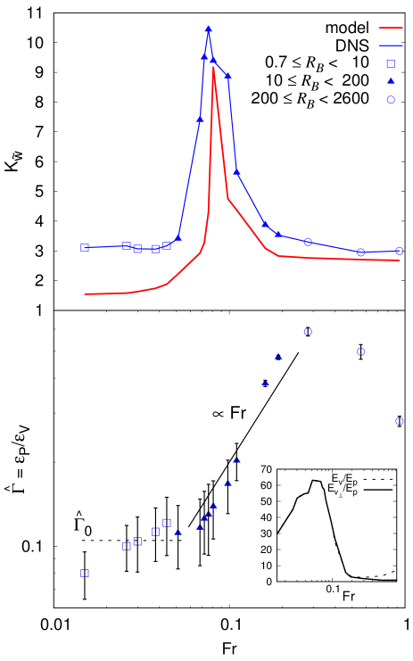
Figure 5: Top: Kurtosis of the Lagrangian vertical velocity $(\tilde{w})$ from the DNS and $(\delta w)$ from the 1D model (red line), as a function of $Fr$. Bottom: irreversible mixing efficiency $\hat{\Gamma}$, with $E_{v}/E_{p}$ and $E_{v_{\perp}}/E_{p}$ in the inset, as a function of $Fr$, all from the DNS; $\hat{\Gamma}_{0}$ is the estimated saturation value obtained in the limit of small Froude numbers. The different symbols are used to identify ranges in terms of the buoyancy Reynolds number $R_{B}$ and highlight the non-monotonic trend of $\hat{\Gamma}$ with $Fr$ and $R_{B}$.

We have shown that very strong and intermittent large-scale vertical drafts can develop in stratified turbulence in a distinct range of Froude number that also reflects an abrupt change in the behavior of the vertical velocity statistics and fluid mixing properties. Similar results of bursty events in the vertical velocity have been obtained in he_15 using DNS of the stable planetary boundary layers with comparable $Re$, no-slip boundary conditions in the vertical direction of a box with an aspect ratio $\sim 10$. These authors find a peak in the number of bursting events for Froude numbers compatible with the range we identified here $(0.05<Fr<0.3)$ in which we observe large-scale intermittency with a peak of the kurtosis of the Lagrangian vertical velocity ($K_{\tilde{w}}$) obtained for $Fr\approx 0.76$. Bursts in stably stratified turbulence were also reported in rorai_14 . In the former case, the observed intermittency is mostly associated with interactions with the boundary, a situation which we do not have in the present study, while in the latter, albeit for only two values of $Fr$, similar extreme events were found. Also, in analysis of climatological data in the free troposphere, it was found that the fields with the strongest departure from Gaussianity are the vertical velocity, together with the specific humidity, and it has been speculated that extreme events in climate behavior such as recent heat waves may be linked to specific resonances in Rossby wave dynamics petoukhov_16 . These results, however, lead to difficulties when mixing efficiency is parameterized. As reported in gregg_18 , results from experiments and numerical simulations attempting characterization of the mixing efficiency fail to converge in many cases. This may be related to the strong non-stationarity of the data for intermediate and small values of $Fr$, as we have shown in Fig.2 ($Fr=0.076$) for the initial phase of evolution of the flow, well beyond the peak of the dissipation.

The present work provides evidence that even without the added complexity of climate processes (including moisture, boundaries and topography) extreme events can be observed in both the vertical velocity and the temperature fluctuations. We also showed how these events are linked to the emergence of structures which in turn correlate, in time and space, with those regions where the flow is more unstable and prone to develop overturning. Our results show that this behavior takes place in a range of Froude numbers relevant for atmospheric and oceanic flows and for values of the buoyancy Reynolds number $>10$. Even though the values of $Re$ considered remain small compared to the troposphere and the ocean, they are not too far off for the mesosphere lower thermosphere (MLT) chau ; marino_15 . Recent numerical studies point also to the possibility that above certain thresholds in $R_{B}$, trends for the mixing efficiency and dissipation represent realistic scenarios even if obtained at $Re$ smaller than those observed in nature pouquet_18 ; marino_15a . Another important result of this Letter is that the observed behavior can be reproduced with a simple 1D model which is a truncation of the full system of governing equations in the Boussinesq framework; this indicates that the the large scale intermittency range in $Fr$ corresponds to a region in the parameter space in which the time scales of waves and nonlinearities near the Ozmidov length-scale are comparable, thus resulting in fast resonant amplification of velocity differences. Finally we found that the irreversible mixing efficiency parameter increases by roughly one order of magnitude (from $\hat{\Gamma}\sim 0.1$ to $\hat{\Gamma}\sim 1$) and scales linearly with the Froude number ($\hat{\Gamma}\propto Fr$) in the range $0.05<Fr<0.3$, relevant for geophysical flows gregg_18 .

References

- (1) Kolmogorov A.N. Dokl. Akad. Nauk SSSR 30 (1941) 9.
- (2) Kolmogorov A.N. J. Fluid Mech. 13 (1962) 82.
- (3) Frisch U. Annals New York Acad. Sci. 357 (1980) 359.
- (4) Fritts D.C. Wang L. J. Geophys. Res. 70 (2013) 3735.
- (5) Falkovich, G. Pumir, A. J. Atmos. Sci. 64 (2007) 4497.
- (6) Bodenschatz E., Malinowski S.P., Shaw R.A. Stratmann F. Science 326 (2010) 970-971.
- (7) Klymak J.M., Pinkel R. Rainville L. J. Phys, Oceanography 38 (2008) 380.
- (8) Pearson B. Fox-Kemper B. Phys. Rev. Lett. 120 (2018) 094501.
- (9) Barkley D., Song B., Mukund V., Lemoult G., Avila M. Hof B. Nature 526 (2015) 550.
- (10) Pumir A., Shraiman B. Siggia E.D. Phys. Rev. Lett. 66 (1991) 2984, Jayesh Warhaft, Z. Phys. Rev. Lett. 67 (1991) 3503.
- (11) Marino R., Sorriso-Valvo L., D’Amicis R., Carbone V., Bruno R. Veltri P. Astrophys. J. 750 (2012) 41.; Marino R., Sorriso-Valvo L., Carbone V., A. Noullez. Bruno R. B. Bavassano Astrophys. J. 677 (2008) L71.
- (12) Chau J.L., Stober G., Hall C.M., Tsutsumi M., Laskar F.I. Hoffmann P. Radio Sci. 52 (2017) 811.
- (13) Mahrt L. J. Atmosph. Sci. 46 (1989) 79.
- (14) D’Asaro E., Lee C., Rainville L., Harcourt R., Thomas L. Science 332 (2011) 318.
- (15) Rorai C., Mininni P.D. Pouquet A. Phys. Rev. E 89 (2014) 043002.
- (16) Rosenberg D., Pouquet A., Marino R. P.Mininni Phys. Fluids 90 (2015) 055105.
- (17) Marino R., Mininni P.D., Rosenberg D., Pouquet A. Phys. Rev. E 90 (2014) 023018., Marino R., Mininni P.D., Rosenberg D., Pouquet A. Eur. Phys. Lett. 102 (2013) 44006.
- (18) Mininni P.D., Rosenberg D., Reddy R. Pouquet A. Parallel Computing 37 (2011) 316.
- (19) Vieillefosse P. Physica A 125 (1984) 150.
- (20) Li Y. Meneveau C. Phys. Rev. Lett. 95 (2005) 164502.
- (21) Ivey G., Winters K. Koseff J. Ann. Rev. Fluid Mech. 40 (2008) 169.
- (22) Pouquet A., Rosenberg D., Marino R. Herbert C. J. Fluid Mech. 844 (2018) 519.
- (23) Shih L., Koseff J., Ivey G. Ferziger J. J. Fluid Mech. 525 (1005) 193.
- (24) Venayagamoorthy S.K. Koseff, J.R. J. Fluid Mech. 798 (2016) R1.
- (25) Mashayek, A., Salehipour, H., Bouffard, D., Caulfield, C.P., Ferrari, R., Nikurashin, M., Peltier, W.R. Smyth, W.D. Geophys. Res. Lett. 44 (2017) 6296.
- (26) Maffioli, A., Brethouwer, G. Lindborg, E. J. Fluid Mech. 794 (2016) R3.
- (27) Osborn T.R. 1980 J. Phys. Oceanogr. 10 (1980) 83-89
- (28) Marino R., Rosenberg D., Herbert C. Pouquet A. Eur. Phys. Lett. 112 (2015) 49001.
- (29) He P. Basu S. Nonlin. Proc. Geophys. 22 (2015) 447.
- (30) Petoukhov V., Petri S., Rahmstorf S., Coumou D., Kornhuber K. Schellnhuber H.J. Proc. Nat. Acad. Sci. 113 (2016) 6862.
- (31) Marino R., Pouquet A. Rosenberg D. Phys. Rev. Lett. 114 (2015) 114504.
- (32) Gregg M.C., D’Asaro E.A., Riley J.J. Kunze E. Ann. Rev. Marine Sci. 10 (2018) 9.