Signals on the power spectra of a cosmology modeled with Chebyshev polynomials

Abstract

We present an interacting model with a phenomenological interaction, $\bar{Q}$, between a cold dark matter (DM) fluid and a dark energy (DE) fluid, which takes a time-varying equation of state (EoS) parameter, $\mathrm{\omega_{DE}}$. Here, both $\bar{Q}$ and $\mathrm{\omega_{DE}}$ are modeled in terms of the Chebyschev polynomials. In a Newtonian gauge and on sub-horizon scales, a set of perturbed equations is obtained when the momentum transfer potential becomes null in the DM rest-frame. This leads to different cases of the interacting model. Then, via a Markov-Chain Monte Carlo (MCMC) method, we constrain such cases by using a combined analysis of geometric and dynamical data. Our results show that in such cases the evolution curves of the structure growth of the matter deviate strongly from the standard model. In addition, we also found that the matter power spectrum is sensitive to $\bar{Q}$. In this way, the coupling modifies the matter scale and generates a slight variation of the turnover point to smaller scales. Likewise, the amplitude of the CMB temperature power spectrum is sensitive the values of $\bar{Q}$ and $\mathrm{\omega_{DE}}$ at low and high multipoles $\it l$, respectively. Here, $\bar{Q}$ can cross twice the line $\bar{Q}=0$ during its background evolution.

1 Introduction

A number of observations Conley2011 ; Jonsson2010 ; Betoule2014 ; Jackson1972 ; Kaiser1987 ; Mehrabi2015 ; Alcock1979 ; Seo2008 ; Battye2015 ; Samushia2014 ; Hudson2013 ; Beutler2012 ; Feix2015 ; Percival2004 ; Song2009 ; Tegmark2006 ; Guzzo2008 ; Samushia2012 ; Blake2011 ; Tojeiro2012 ; Reid2012 ; delaTorre2013 ; Planck2015 ; Hinshaw2013 ; Beutler2011 ; Ross2015 ; Percival2010 ; Kazin2010 ; Padmanabhan2012 ; Chuang2013a ; Chuang2013b ; Anderson2014a ; Kazin2014 ; Debulac2015 ; FontRibera2014 ; Eisenstein1998 ; Eisenstein2005 ; Hemantha2014 ; Bond-Tegmark1997 ; Hu-Sugiyama1996 ; Neveu2016 ; Sharov2015 ; Zhang2014 ; Simon2005 ; Moresco2012 ; Gastanaga2009 ; Oka2014 ; Blake2012 ; Stern2010 ; Moresco2015 ; Busca2013 have indicated that the present universe is undergoing a phase of accelerated expansion, and driven probably by a new form of energy with negative EoS parameter, commonly so-called DE DES2006 . This energy has been interpreted in various forms and widely studied in OptionsDE . However, within General Relativity (GR) the DE models can suffer the coincidence problem, namely why the DM and DE energy densities are of the same order today. This latter problem could be solved or even alleviated, by assuming the existence of a non-gravitational $\bar{Q}$ within the dark sector, which gives rise to a continuous energy exchange from DE to DM or vice-versa. Currently, there are n’t neither physical arguments nor recent observations to exclude $\bar{Q}$ Interacting ; Pavons ; Wangs ; Cueva-Nucamendi2012 . Moreover, due to the absence of a fundamental theory to construct $\bar{Q}$, different ansatzes have been widely discussed in Interacting ; Pavons ; Wangs ; Cueva-Nucamendi2012 ; valiviita2008 ; Clemson2012 . So, It has been shown in some coupled DE scenarios that $\bar{Q}$ can affect the background evolution of the DM density perturbations and the expansion history of the universe Mehrabi2015 ; valiviita2008 ; Clemson2012 ; Alcaniz2013 ; Yang2014 . Thus, $\bar{Q}$ and $\mathrm{\omega_{DE}}$ could very possibly introduce new features on the evolution curves of the structure growth of the matter, on the linear matter power spectrum and on the amplitude of the CMB temperature power spectrum at low and high multipoles, respectively Mehrabi2015 ; Clemson2012 ; Alcaniz2013 ; Yang2014 ; Mota2017 .
On the other one, within dark sector we can propose new ansatzes for both $\bar{Q}$ and $\mathrm{\omega_{DE}}$, which can be expanded in terms of the Chebyshev polynomials $T_{n}$, defined in the interval $[-1,1]$ and with a divergence-free $\mathrm{\omega_{DE}}$ at z$\rightarrow-1$ Chevallier-Linder ; Li-Ma . However, that polynomial base was particularly chosen due to its rapid convergence and better stability than others, by giving minimal errors Simon2005 ; Martinez2008 . Besides, $\bar{Q}$ could also be proportional to the DM energy density $\mathrm{{\bar{\rho}}_{DM}}$ and to the Hubble parameter $\bar{H}$. This new model will guarantee an accelerated scaling attractor and connect to a standard evolution of the matter. Here, $\bar{Q}$ will be res-tricted from the criteria exhibit in Campo-Herrera2015 .
The focus of this paper is to investigate the effects of $\bar{Q}$ and $\mathrm{\omega_{DE}}$ on the curves of structure growth, on the ma-tter power spectrum and on the CMB temperature power spectrum including the search for a new way to alleviate the coincidence problem.
On the other hand, an interacting DE model is discussed, on which we have performed a global fitting, by using an analysis combined of Joint Light Curve Analysis (JLA) type Ia Supernovae (SNe Ia) data Conley2011 ; Jonsson2010 ; Betoule2014 , including the growth rate of structure formation obtained from redshift space distortion (RSD) data Jackson1972 ; Kaiser1987 ; Mehrabi2015 ; Alcock1979 ; Seo2008 ; Battye2015 ; Samushia2014 ; Hudson2013 ; Beutler2012 ; Feix2015 ; Percival2004 ; Song2009 ; Tegmark2006 ; Guzzo2008 ; Samushia2012 ; Blake2011 ; Tojeiro2012 ; Reid2012 ; delaTorre2013 ; Planck2015 , together with Baryon Acoustic Oscillation (BAO) data Hinshaw2013 ; Beutler2011 ; Ross2015 ; Percival2010 ; Kazin2010 ; Padmanabhan2012 ; Chuang2013a ; Chuang2013b ; Anderson2014a ; Kazin2014 ; Debulac2015 ; FontRibera2014 ; Eisenstein1998 ; Eisenstein2005 ; Hemantha2014 , as well as the observations of anisotropies in the power spectrum of the Cosmic Microwave Background (CMB) data Planck2015 ; Bond-Tegmark1997 ; Hu-Sugiyama1996 ; Neveu2016 and the Hubble parameter (H) data obtained from galaxy surveys Sharov2015 ; Zhang2014 ; Simon2005 ; Moresco2012 ; Gastanaga2009 ; Oka2014 ; Blake2012 ; Stern2010 ; Moresco2015 ; Busca2013 to constrain the parameter space of such model and break the degeneracy of their parameters, putting tighter constraints on them.
Finally, we organize this paper as follows: We describe the background equations of the interacting DE model in Sec. II, the perturbed equations, the modified growth factor, the linear matter and CMB temperature power spectra in Sec. III. The constraint method and observational data are presented in Sec. IV. We discuss our results in Sec. V and show our conclusions in Sec. VI.

2 Interacting dark energy (IDE) model

We assume a spatially flat Friedmann-Robertson-Walker (FRW) universe, composed with four perfect fluids-like, radiation (subscript r), baryonic matter (subscript b), DM and DE, respectively. Moreover, we postulate the existence of a non-gravitational coupling in the background between DM and DE (so-called dark sector) and two decoupled sectors related to the b and r components, respectively. We also consider that these fluids have EoS parameters ${\mathrm{P}}_{A}=\mathrm{\omega}_{A}\mathrm{\bar{\rho}}_{A}$, $A=b,r,DM,DE$, where $\mathrm{P}_{A}$ and $\mathrm{{\bar{\rho}}}_{A}$ are the corresponding pressures and the energy densities. Here, we choose $\mathrm{\omega_{DM}=\omega_{b}=0}$, $\mathrm{\omega_{r}=1/3}$ and $\mathrm{\omega_{DE}}$ is a time-varying function. Therefore, the balance equations of our fluids are respectively,

$$\frac{\mathrm{d}\bar{\rho}_{b}}{\mathrm{d}z}-3{\bar{H}}{\bar{\rho}}_{b} = 0,$$ (1)

$$\frac{\mathrm{d}\bar{\rho}_{r}}{\mathrm{d}z}-4{\bar{H}}{\bar{\rho}}_{r} = 0,$$ (2)

$$\frac{\mathrm{d}\bar{\rho}_{DM}}{\mathrm{d}z}-\frac{3{\bar{\rho}}_{DM}}{(1+z)} = -\frac{\bar{Q}}{\bar{H}(1+z)},$$ (3)

$$\frac{\mathrm{d}\bar{\rho}_{DE}}{\mathrm{d}z}-\frac{3(1+\omega_{DE}){\bar{\rho}}_{DE}}{(1+z)} = +\frac{\bar{Q}}{\bar{H}(1+z)},$$ (4)

where the differentiation has been done with respect to the redshift, $\mathrm{z}$, $\bar{H}$ denotes the Hubble expansion rate and the quantity $\bar{Q}$ expresses the interaction between the dark sectors. For simplicity, it is convenient to define the fractional energy densities $\mathrm{{\bar{\Omega}}_{i}}\equiv\frac{\mathrm{\bar{\rho}_{A}}}{\rho_{c}}$ and ${\mathrm{\Omega}}_{A,0}\equiv\frac{{\rho}_{i,0}}{\rho_{c,0}}$, where the critical density $\rho_{c}\equiv 3{\bar{H}}^{2}/8\pi G$ and the critical density today $\rho_{c,0}\equiv 3\mathrm{H_{0}}^{2}/8\pi G$ being $\mathrm{H_{0}}=100h\,Kms^{-1}Mpc^{-1}$ the current value of $\bar{H}$. Likewise, we have taken the relation $\mathrm{{\bar{\Omega}}_{b,0}+{\bar{\Omega}}_{r,0}+{\bar{\Omega}}_{DM,0}+{\bar{\Omega}}_{DE,0}=1}$. Here, the subscript “0” indicates the present day value of the quantity.
In this work, we consider the spatially flat FRW metric with line element

$${\rm ds}^{2}=-{\rm d}{t}^{2}+{\mathrm{\bf a}}^{2}(t)\delta_{ij}d{x}^{i}d{x}^{j},$$ (5)

where $t$ represents the cosmic time and “$\mathrm{\bf a}$” represents the scale factor of the metric and it is defined in terms of the redshift $\mathrm{z}$ as $\mathrm{\bf a}=(1+\mathrm{z})^{-1}$.
Here, we analyze the ratio between the energy densities of DM and DE, defined as $\mathrm{R}\equiv\mathrm{{\bar{\rho}}_{DM}}/\mathrm{{\bar{\rho}}_{DE}}$. From Eqs. (3) and (4), we obtain Campo-Herrera2015 ; Ratios

$$\frac{\mathrm{d}R}{\mathrm{d}z}=\frac{-R}{(1+z)}\left(3\omega_{DE}+\frac{(1+R)\bar{Q}}{\bar{H}\rho_{DM}}\right).$$ (6)

This Eq. leads to

$$\bar{Q}=-\left(3\omega_{DE}+\frac{\mathrm{d}R}{\mathrm{d}z}\frac{(1+z)}{R}\right)\frac{\bar{H}{\bar{\rho}}_{DM}}{1+R}.$$ (7)

Due to the fact that the origin and nature of the dark fluids are unknown, it is not possible to derive $\bar{Q}$ from fundamental principles. However, we have the freedom of choosing any possible form of $\bar{Q}$ that satisfies Eqs. (3) and (4) simultaneously. Hence, we propose a phenomenological description for $\bar{Q}$ as a linear combination of $\mathrm{{\bar{\rho}}_{DM}}$, ${\bar{H}}$ and a time-varying function ${\bar{\rm I}}_{\rm Q}$,

$${\bar{Q}}\equiv\mathrm{\bar{H}}\mathrm{\bar{\rho}_{DM}}\bar{{\rm I}}_{\rm Q},\qquad{\bar{\rm I}}_{\rm Q}\equiv\sum_{n=0}{{\lambda}}_{n}T_{n},$$ (8)

where ${\bar{\rm I}}_{\rm Q}$ is defined in terms of Chebyshev polynomials and $\mathrm{{\lambda}_{n}}$ are constant and small $|\mathrm{{\lambda}_{n}}|\ll 1$ dimensionless parameters. This polynomial base was chosen because it converges rapidly, is more stable than others and behaves well in any polynomial expansion, giving minimal errors Cueva-Nucamendi2012 . The first three Chebyshev polynomials are

$$T_{0}(z)=1\;,\hskip 8.5359ptT_{1}(z)=z\;,\hskip 8.5359ptT_{2}(z)=(2z^{2}-1).$$ (9)

From Eqs. (8) and (9) an asymptotic value for ${\bar{\rm I}}_{\rm Q}$ can be found: ${\bar{\rm I}}_{\rm Q}\rightarrow\infty$ for $\mathrm{z}\rightarrow\infty$, ${\bar{\rm I}}_{\rm Q}=\mathrm{{\lambda}_{0}-{\lambda}_{2}}$ for $\mathrm{z}=0$ and ${\bar{\rm I}}_{\rm Q}\approx\mathrm{{\lambda}_{0}-{\lambda}_{1}+{\lambda}_{2}}$ for $\mathrm{z}\rightarrow-1$.
Similarly, we will focus on an interacting model with a specific ansatz for the EoS parameter, given as

$$\mathrm{\omega_{DE}}\equiv\omega_{2}+2\sum^{2}_{m=0}\frac{\omega_{m}T_{m}}{2+{\mathrm{z}}^{2}}.$$ (10)

Within this ansatz a finite value for $\omega$ is obtained from the past to the future; namely, the following asymptotic values are found: $\mathrm{\omega_{DE}}=5\omega_{2}$ for $\mathrm{z}\rightarrow\infty$, $\mathrm{\omega_{DE}}\approx\omega_{0}$ for $\mathrm{z}=0$ and $\mathrm{\omega_{DE}}\approx(5/3)\omega_{2}+(2/3)[\omega_{0}-\omega_{1}]$ for $\mathrm{z}\rightarrow-1$. Therefore, a possible physical description should be studied to explore its properties.
In order to guarantee that $\bar{Q}$ may be physically acceptable in the dark sectors Campo-Herrera2015 , we equal the right-hand sides of Eqs. (7) and (8), which becomes

$$\frac{\mathrm{dR}}{\mathrm{d}z}=\frac{-\mathrm{R}}{(1+\mathrm{z})}\biggl{(}{\bar{\rm I}}_{\rm Q}(1+\mathrm{R})+3\mathrm{{\omega}_{DE}}\biggr{)}.$$ (11)

Now, to solve or alleviate of coincidence problem, we require that $\mathrm{R}$ tends to a fixed value at late times. This leads to the condition ${\mathrm{dR}}/{\mathrm{dz}}=0$, which therefore implies two stationary solutions $\mathrm{R_{+}}=\mathrm{R(z\rightarrow\infty)}=-(1+{3\mathrm{\omega_{DE}}}/{{\bar{\rm I}}_{\rm Q}})$ and $\mathrm{R_{-}}=\mathrm{R(z\rightarrow-1)}=0$, The first solution occurs in the past and the second one happens in the future.
By inserting Eqs. (8) and (10) into Eq. (11), we find that $\mathrm{R}$ has no analytical solution, in any case, it is to be solved numerically. Likewise, there are an analytical solution for just $\mathrm{{\bar{\rho}}_{b}}$, $\mathrm{{\bar{\rho}}_{r}}$ and $\mathrm{{\bar{\rho}}_{DM}}$, respectively, but $\mathrm{{\bar{\rho}}_{DE}}$ will be obtained from $\mathrm{R}$, as $\mathrm{{\bar{\rho}}_{DE}}=\mathrm{{\bar{\rho}}_{DM}}/\mathrm{R}$.
Therefore, the first Friedmann equation is given by

$$\vskip 3.0pt plus 1.0pt minus 1.0ptE^{2}=\frac{{\bar{H}}^{2}}{\mathrm{{H}^{2}_{0}}}=\mathrm{\Omega_{b,0}}{(1+\mathrm{z})}^{3}+\mathrm{\Omega_{r,0}}{(1+\mathrm{z})}^{4}\\ +\mathrm{\Omega^{\star}_{DM}}(\mathrm{z})(1+{\mathrm{R}}^{-1}),$$ (12)

where have considered that

$$\vskip 3.0pt plus 1.0pt minus 1.0pt\mathrm{\Omega^{\star}_{DM}}(\mathrm{z})=(1+\mathrm{z})^{3}{\mathrm{\Omega_{DM,0}}}{\rm exp}\biggl{[}{\frac{-z_{max}}{2}\sum_{n=0}^{2}\lambda_{n}I_{n}(\mathrm{z})}\biggr{]},\qquad\qquad\qquad$$

$$\int_{0}^{\mathrm{z}}\frac{T_{n}(\tilde{x})}{(1+\tilde{x})}d\tilde{x}\,\approx\,\frac{z_{max}}{2}\int_{-1}^{x}\frac{T_{n}(\tilde{x})}{(a_{1}+a_{2}\tilde{x})}d\tilde{x}\equiv\frac{z_{max}}{2}I_{n}(\mathrm{z}),\qquad\qquad$$

$$x\,\equiv\,\frac{2\mathrm{z}}{z_{max}}-1,\quad a_{1}\equiv 1+\frac{z_{max}}{2}\,,\quad a_{2}\equiv\frac{z_{max}}{2},\qquad\qquad\qquad$$

$$I_{0}(\mathrm{z})=\frac{2}{z_{max}}\ln(1+\mathrm{z}),\qquad\qquad\qquad\qquad\qquad\qquad\qquad\qquad\qquad$$

$$I_{1}(\mathrm{z})=\,\frac{2}{z_{max}}\biggl{(}\frac{2\mathrm{z}}{z_{max}}-\frac{(2+z_{max})}{z_{max}}\ln(1+\mathrm{z})\biggr{)},\qquad\qquad\qquad\qquad$$

$$I_{2}(\mathrm{z})\,=\,\frac{2}{z_{max}}\biggl{[}\frac{4\mathrm{z}}{z_{max}}\biggl{(}\frac{\mathrm{z}}{z_{max}}-\frac{2}{z_{max}}-2\biggr{)}+\qquad\qquad\qquad\qquad\quad$$

$$\biggl{(}1+\frac{6.8284}{z_{max}}\biggr{)}\biggl{(}1+\frac{1.1716}{z_{max}}\biggr{)}\ln(1+\mathrm{z})\biggr{]},\hskip 85.35826pt$$

where $z_{max}$ is the maximum value of $\mathrm{z}$ such that $\tilde{x}\in[-1,1]$ and $|{T_{n}}(\tilde{x})|\leq 1$ and $n\in[0,2]$ Cueva-Nucamendi2012 .
If $\bar{Q}(z)=0$ and $\mathrm{\omega_{DE}}=-1$ in Eq. (12) the standard $\Lambda$CDM model is recovered. Similarly, when $\bar{Q}(z)=0$ and $\mathrm{\omega_{DE}}$ are nonzero, the $\omega$DE model is obtained. These non-interacting models have an analytical solution for $\mathrm{R}$.

3 IDE in the perturbed universe

3.1 Perturbed equations

In the Newtonian gauge, the perturbed FRW metric becomes valiviita2008 ; Clemson2012

$${\rm ds}^{2}=\biggl{[}-\left(1+2\phi\right){\rm d}{t}^{2}+{\mathrm{\bf a}}^{2}(t)\left(1-2\psi\right)\delta_{ij}d{x}^{i}d{x}^{j}\biggr{]},$$ (13)

where $\phi$ and $\psi$ are gravitational potentials, and the four-velocity of fluid $A$ ($A=$ DM, DE, b, r) is

$$U^{\mu}_{A}={\mathrm{\bf a}}^{-1}(1-\phi,\partial^{i}v_{A})\,,\quad U_{\mu}^{A}={\mathrm{\bf a}}(-1-\phi,\partial_{i}v_{A}),$$ (14)

where $v_{A}$ is the peculiar velocity potential, and $\theta_{A}$ is the velocity perturbation defined as $\theta_{A}=-k^{2}v_{A}$.
The energy-momentum conservation equation of $A$ fluid in interaction is given by valiviita2008 ; Clemson2012

$$\nabla_{\nu}{T_{A}}^{\mu\nu}=Q_{A}^{\mu},\,\,\,Q_{DM}^{\mu}=-Q_{DE}^{\mu}\neq 0=Q_{b}^{\mu}=Q_{r}^{\mu},$$ (15)

where ${T_{A}}^{\mu\nu}$ is the $A$-fluid energy momentum tensor.
In general, $Q_{A}^{\mu}$ can be split relative to the total four-velocity $U^{\mu}$ as valiviita2008 ; Clemson2012

$$Q_{A}^{\mu} = {Q}_{A}U^{\mu}_{A}+F^{\mu}_{A},\quad Q_{A}=\bar{Q}_{A}+\delta Q_{A},\quad U_{\mu}^{A}F^{\mu}_{A}=0,$$

$$\bar{Q}_{DM} = -\bar{Q}_{DE}\neq 0=\bar{Q}_{b}=-\bar{Q}_{r},$$

$$\delta{Q}_{DM} = -\delta{Q}_{DE}\neq 0=\delta{Q}_{b}=-\delta{Q}_{r},$$ (16)

where ${Q}_{A}$ and $F^{\mu}_{A}$ represent the energy and momentum transfer rate, respectively, relative to $U^{\mu}_{A}$. Likewise, to the first order $F^{\mu}_{A}={\mathrm{\bf a}}^{-1}(0,\partial^{i}f_{A})$ where $f_{A}$ is a momentum transfer potential and $\bar{Q}_{A}$ represents the interaction term. From Eqs. (14) and (3.1), we find Clemson2012

$$Q^{A}_{0}=-{\mathrm{\bf a}}\left[\bar{Q}_{A}(1+\phi)+\delta{Q_{A}}\right],\quad Q^{A}_{i}={\mathrm{\bf a}}\partial_{k}\left[f_{A}+\bar{Q}_{A}v\right],$$ (17)

with $\bar{Q}_{DM}=-\bar{Q}_{DE}\neq 0$ and $\delta{Q}_{DM}=-\delta{Q}_{DE}$.
Here, we have considered that the $A$ fluid physical sound speed in the rest-frame defined by $c_{sA}^{2}\equiv\delta{{P}_{A}}/\delta{\rho}_{A}{\mid}_{rf}$ and the adiabatic sound speed is defined by $c_{{\bf\mathrm{a}}A}^{2}\equiv{\partial{P}_{A}}/{\partial{\rho}_{A}}=\mathrm{\omega_{A}}+(\frac{\mathrm{d}{\omega}_{A}}{\mathrm{d}z}/\frac{\mathrm{d}{\bar{\rho}_{A}}}{\mathrm{d}z})\mathrm{\bar{\rho}_{A}}$ Then, for the adiabatic DM fluid, we take $c^{2}_{sDM}=c^{2}_{{\bf\mathrm{a}}DM}=\mathrm{\omega_{DM}}=0$. Instead, for the non-adiabatic DE fluid, $c^{2}_{\mathrm{aDE}}=\mathrm{\omega_{DE}}<0$ and the physical sound speed for DE is usually considered as $c^{2}_{sDE}=1$ to eliminate possible unphysical instabilities.
Immediately, we have established the simpler physical choice for the momentum transfer potential between the dark sectors, which happens when $f_{A}=0$ in the rest-frame of either DM or DE valiviita2008 . Consequently, this choice allows two different possibilities for $Q_{A}^{\mu}$ and $f_{A}$, which can be parallel to either the DM or the DE four velocity, respectively. In this work, we focus only on the case valiviita2008 ; Clemson2012

$${Q}_{DE}^{\mu}={\bar{Q}}_{DE}U^{\mu}_{DM} = -{Q}_{DM}^{\mu},\quad Q^{\mu}_{A}\parallel U^{\mu}_{DM},\qquad$$

$$f_{DM}=\frac{{\bar{Q}}_{A}}{k^{2}}(\theta-\theta_{DM}) = -f_{DE}\,,\,\quad Q^{\mu}_{A}\parallel U^{\mu}_{DM},$$ (18)

On the other hand, assuming that $\bar{Q}$ depends on the cosmic time through the global expansion rate, then a possible choice for $\delta{\bar{H}}$ can be $\delta{\bar{H}}=0$. Likewise, for convenience, we impose that ${{\delta{\rm I}}_{\rm Q}}\ll{\delta_{DM}}$, it leads to

$${\delta Q}_{DM}=-{\bar{H}}{\bar{\rm I}}_{\rm Q}\mathrm{{\bar{\rho}}_{DM}}{\delta}_{DM}\;.$$ (19)

In a forthcoming article we will extend our study, by considering other relations between ${{\delta{\rm I}}_{\rm Q}}$, ${\delta_{DM}}$ and $\delta{H}$. It is beyond the scope of the present paper.
In this work, we are interested in studying the effects of $\mathrm{\omega_{DE}}$ and $\bar{Q}$ on the total matter power spectrum and on the CMB temperature power spectrum. For this reason, we consider only the adiabatic perturbations, assume that ${T_{A}}^{\mu\nu}$ is free of anisotropic stress, and the arguments above discussed, we find the evolution equations for the density contrast perturbation $\delta_{A}$ and the velocity perturbations $\theta_{A}$ in the IDE model from the general case presented in valiviita2008 ; Clemson2012 when $Q^{\mu}_{A}\parallel U^{\mu}_{DM}$,

$$\frac{\mathrm{d}{\delta}_{DE}}{\mathrm{d}z} = -(\mathrm{R}{\bar{\rm I}}_{\rm Q}-3+3\mathrm{\omega_{DE}})\frac{\delta_{DE}}{(1+\mathrm{z})}+(1+\mathrm{\omega_{DE}})\frac{\theta_{DE}}{\bar{H}}$$ (20)

$$+\frac{\bar{H}\theta_{DE}}{(1+\mathrm{z})^{2}\mathrm{k^{2}}}\biggl{[}9(1-\mathrm{{\omega}_{DE}^{2}})-3(1+\mathrm{z})\frac{\mathrm{d}{\omega}_{DE}}{\mathrm{d}z}$$

$$+3\mathrm{R}{\bar{\rm I}}_{\rm Q}(1-\mathrm{\omega_{DE}})\biggr{]}+3(1+\mathrm{\omega_{DE}})\frac{\mathrm{d}{\psi}}{\mathrm{d}z}+$$

$$+\frac{\mathrm{R}{\bar{\rm I}}_{\rm Q}\phi}{(1+\mathrm{z})}+\frac{\mathrm{R}{\bar{\rm I}}_{\rm Q}}{(1+\mathrm{z})}\delta_{DM},$$

$$\frac{\mathrm{d}{\delta}_{DM}}{\mathrm{d}z} = \frac{\theta_{DM}}{\bar{H}}-\frac{{\bar{\rm I}}_{\rm Q}\phi}{(1+\mathrm{z})}+3\frac{\mathrm{d}{\psi}}{\mathrm{d}z}\,,$$ (21)

$$\frac{\mathrm{d}{\delta}_{b}}{\mathrm{d}z} = \frac{\theta_{b}}{\bar{H}}+3\frac{\mathrm{d}{\psi}}{\mathrm{d}z},$$ (22)

$$\frac{\mathrm{d}{\theta}_{DE}}{\mathrm{d}z} = -\frac{2{{\theta}_{DE}}}{(1+\mathrm{z})}\left(1+\frac{\mathrm{R}{\bar{\rm I}}_{\rm Q}}{(1+\mathrm{\omega_{DE}})}\right)-\frac{\mathrm{k^{2}}{\delta}_{DE}}{\bar{H}(1+\mathrm{\omega_{DE}})}$$ (23)

$$-\frac{\mathrm{k^{2}}\phi}{\bar{H}}+\frac{\mathrm{R}{\bar{\rm I}}_{\rm Q}{\theta}_{DM}}{(1+\mathrm{z})(1+\mathrm{\omega_{DE}})},$$

$$\frac{\mathrm{d}{\theta}_{DM}}{\mathrm{d}z} = \frac{\theta_{DM}}{(1+\mathrm{z})}-\frac{k^{2}\phi}{\bar{H}},$$ (24)

$$\frac{\mathrm{d}{\theta}_{b}}{\mathrm{d}z} = \frac{\theta_{b}}{(1+\mathrm{z})}-\frac{k^{2}\phi}{\bar{H}}.$$ (25)

Furthermore, the relativistic Poisson equation is given by

$$\mathrm{k}^{2}\phi = \frac{3\bar{H}^{2}}{(1+\mathrm{z})}\frac{\mathrm{d}{\psi}}{\mathrm{d}z}-\frac{3{\bar{H}}^{2}\phi}{(1+\mathrm{z})^{2}}-\frac{4\pi G}{(1+\mathrm{z})^{2}}\times$$ (26)

$$\biggl{(}\bar{\rho}_{b}\delta_{b}+\bar{\rho}_{DM}\delta_{DM}+\bar{\rho}_{DE}\delta_{DE}+\bar{\rho}_{r}\delta_{r}\biggr{)}.$$

3.2 Structure formation

In the Newtonian limit ($\delta\ll 1$) and at sub-horizon scales ($\bar{H}^{2}\ll\mathrm{k}^{2}$), we assume that DE fluid does not contribute in clustering of matter and therefore we could take $\delta_{DM}\gg\delta_{DE}\approx 0$. Besides, for simplicity, we also consider that the gravitational potentials $\phi$ and $\psi$, satisfy $\delta_{DM}\gg\phi=\psi$ and $\phi^{\prime}=\psi^{\prime}\approx 0$.
Since we are only interested in showing the effects of $\bar{Q}$ and $\mathrm{{\omega}_{DE}}$ on the evolution of $\delta_{DM}$ during the matter dominated era, rather than making accurate calculations. Again, for simplicity, we can ignore the contribution of the radiation in our estimations. Due to the arguments above discussed and combining Eqs. (21), (24) and (26), we obtain

$$\frac{\mathrm{d}^{2}{\delta}_{DM}}{\mathrm{d}{\mathrm{z}}^{2}} = -\frac{(1+3\mathrm{\omega_{DE}}\mathrm{\bar{\Omega}_{DE}}+\mathrm{\bar{\Omega}_{r}})}{2(1+\mathrm{z})}\frac{\mathrm{d}{\delta}_{DM}}{\mathrm{dz}}$$ (27)

$$+\frac{3}{2(1+\mathrm{z})^{2}}\biggl{(}\mathrm{\bar{\Omega}_{DM}}\delta_{DM}+\mathrm{\bar{\Omega}_{b}}\delta_{b}\biggr{)}.$$

A similar equation can be obtained for $\delta_{b}$.
Next, we define the growth factor of linear matter perturbations as

$$\mathrm{f}\equiv\frac{{d}{\ln}\delta_{\mathrm{M}}}{d{\ln\mathrm{\bf a}}}\,,\quad{{\delta}_{\mathrm{M}}=\mathrm{\Omega_{DM}}\delta_{DM}+\mathrm{\Omega_{b}}\delta_{b}},$$ (28)

where ${\delta}_{\mathrm{M}}$ is the normalized matter density perturbations.
Via the above definition and by considering that $\delta_{b}\ll\delta_{DM}$, Eq. (27) can be re-expressed in terms of the redshift for the case $Q^{\mu}_{A}\parallel U^{\mu}_{DM}$, as

$$\frac{d\mathrm{f}}{d\mathrm{z}}=\frac{1}{\mathrm{(1+z)}}\biggl{[}\mathrm{f}^{2}+\frac{\mathrm{f}}{2}\left(1-3\mathrm{\omega_{DE}}\mathrm{\bar{\Omega}_{DE}}-\mathrm{\bar{\Omega}_{r}}\right)-\frac{3}{2}\mathrm{\bar{\Omega}_{DM}}\biggr{]}.$$ (29)

An analytical solution to Eq. (29) is very complicated to obtain, and we need to use numerical methods. For this reason, it is most suitable to approach $\mathrm{f}$ in the form

$$\mathrm{f}={\bar{\Omega}_{M}}^{\gamma}\,,$$ (30)

where $\gamma$ is the growth index of the linear matter fluctuations, and in general is a function of the redshift or scale factor. Hence, Eq. (27) can be solved numerically taking into account the conditions at $\mathrm{z}=0$: $\mathrm{\delta_{M,0}|=1}$ and ${\mathrm{d{\delta}_{M}}}/{\mathrm{dz}}|_{\mathrm{z}=0}=-\mathrm{\Omega_{M,0}}^{\mathrm{\gamma_{0}}}$, where $\Omega_{M,0}$ and $\gamma_{0}$ are the values today, and $\mathrm{\Omega_{M,0}}=\mathrm{\Omega_{DM,0}+\Omega_{b,0}}$.
Similarly, by considering the condition $\mathrm{f_{0}}=\mathrm{{\Omega_{M,0}}^{\gamma_{0}}}$, Eq. (29) can also be solved numerically.
On the other hand, the root-mean-square amplitude of matter density perturbations within a sphere of radius $\mathrm{8\,Mpc}h^{-1}$ is denoted as $\mathrm{\sigma_{8}(z)}$ and its evolution is represented by

$$\mathrm{\sigma_{8}(z)}=\delta_{M}(\mathrm{z})\mathrm{\sigma_{8,0}},$$ (31)

where $\mathrm{\sigma_{8,0}}$ is the normalizations to unity of $\mathrm{\sigma_{8}(z)}$ today. Thus, the functions $\mathrm{f}$ y $\mathrm{\sigma_{8}}$ can be combined to obtain $\mathrm{f\sigma_{8}}$ at different redshifts. From here, we obtain

$$\mathrm{f(z)\sigma_{8}(z)}=\mathrm{f(z)}\delta(\mathrm{z})\mathrm{\sigma_{8,0}}.$$ (32)

3.3 Linear matter power spectrum.

The linear matter power spectrum $\mathrm{P(k,z)}$ is Hu1998 ; Dodelson2003

$$\mathrm{P(k,z)}=2\pi^{2}\mathrm{H_{0}}^{-(3+n_{s})}\delta_{H}^{2}k^{n_{s}}T^{2}(\mathrm{k})\delta_{M}^{2}(\mathrm{z}),$$ (33)

where ${T(\mathrm{k})}$ is the transfer function, $n_{s}$ is the scalar spectral index of the primordial fluctuation spectrum, $\mathrm{k}$ is the wavenumber and $\delta_{H}$ is defined Hu1998 ; Dodelson2003 by

$$\delta_{H}\approx 1.94\times 10^{-5}\mathrm{\Omega_{M,0}}^{-0.785-0.05\mathrm{\ln\Omega_{M,0}}}e^{-0.95(n_{s}-1)}.\,\,$$ (34)

In this work, we adopt the fitting formula proposed in Hu1998 ; Dodelson2003 that approximates the full transfer function as the sum of the baryon and cold DM contribution on all scales

$$T(\mathrm{k})=\mathrm{\frac{\Omega_{b,0}}{\Omega_{M,0}}}T_{b}(\mathrm{k})+\mathrm{\frac{\Omega_{DM,0}}{\Omega_{M,0}}}T_{DM}(\mathrm{k}).$$ (35)

Here, $T_{b}(k)$ is the baryon transfer function defined as

$$T_{b}(\mathrm{k}) = \biggl{[}\frac{1}{1+(\frac{\mathrm{k}r_{d}}{5.2})^{2}}\frac{\ln(e+1.8q)}{\ln(e+1.8q)+C_{0}q^{2}}+$$

$$\frac{\alpha_{b}e^{-(\mathrm{k/k_{silk}})^{1.4}}}{1+(\beta_{b}/\mathrm{k}r_{d})^{3}}\biggr{]}\frac{sin(\mathrm{k}\tilde{r})}{\mathrm{k}\tilde{r}},$$

$$q = \frac{\mathrm{k}}{13.41\mathrm{k_{eq}}},\quad\alpha_{b}=\frac{2.07\mathrm{k_{eq}}r_{d}G}{(1+R_{d})^{0.75}}\frac{\mathrm{a_{*}}}{\mathrm{a_{eq}}},$$

$$r_{d} = \frac{2}{3\mathrm{k_{eq}}}\sqrt{\frac{6}{R_{eq}}}\ln\biggl{[}\frac{\sqrt{R_{d}+R_{eq}}+\sqrt{1+R_{d}}}{1+\sqrt{R_{eq}}}\biggr{]},$$

$$\tilde{r} = \frac{r_{d}}{[1+(\frac{\beta_{node}}{\mathrm{k}r_{d}})^{3}]^{1/3}}\quad\beta_{node}=8.41(\mathrm{\Omega_{m0}}h^{2})^{0.435},$$

$$\mathrm{k_{silk}} = 1.6(\mathrm{\Omega_{b0}}h^{2})^{0.52}(\mathrm{\Omega_{m0}}h^{2})^{0.73}\biggl{[}1+\frac{1}{(10.4\mathrm{\Omega_{m0}}h^{2})^{0.95}}\biggr{]},$$

$$\mathrm{\beta_{b}} = 0.5+\mathrm{\frac{\Omega_{b,0}}{\Omega_{m0}}+(3-\frac{2\Omega_{b0}}{\Omega_{m0}})}\sqrt{(17.2\mathrm{\Omega_{m0}}h^{2})^{2}+1},\,$$ (36)

where $R_{d}$ is the ratio of the baryon to photon energy density at the drag epoch, $\mathrm{k_{eq}}$ is the wave-number at the equality epoch radiation-matter, $r_{d}(z_{d})$ is the sound horizon at the drag epoch, $G$ is a factor of suppression, $\mathrm{a_{*}}$ represents the scale factor at the recombination epoch, $\mathrm{a_{eq}}$ represents the scale factor at the equality epoch radiation-matter and $\mathrm{k_{silk}}$ represents the Silk damping scale Hu1998 ; Dodelson2003 .
Similarly, the cold DM transfer function, $T_{DM}(\mathrm{k})$, is defined as Hu1998 ; Dodelson2003 .

$$T_{DM}(\mathrm{k}) = \frac{{L_{0}}}{{L_{0}+C_{0}q^{2}}}\,,\quad{L_{0}}={\ln(5.436+1.8q)},$$

$${C_{0}} = 14.2+\frac{731}{1+62.5{q}},\quad{q}=\frac{\mathrm{k}}{h\Gamma},$$ (37)

and the shape parameter $\Gamma$, is given by Hu1998 ; Dodelson2003

$$\Gamma\equiv\mathrm{\Omega_{M,0}}h\left(\zeta+\frac{1-\zeta}{[1+0.43\mathrm{k}r_{s}(z_{d})]^{4}}\right),\,\,\upsilon=\mathrm{\frac{\Omega_{b,0}}{\Omega_{M,0}}},\quad$$ (38)

$$\zeta=1-0.328\ln(431\mathrm{\Omega_{M,0}}h^{2})\upsilon+0.38\ln(22.3\mathrm{\Omega_{M,0}}h^{2})\upsilon^{2}.$$

3.4 CMB temperature power spectrum.

From Eqs. (33)-(3.3), using the results found in Dodelson2003 and the Limber approximation Limber1953 , we have built numerically the CMB temperature power spectrum today as

$$C_{l}\,\alpha\,\frac{B_{1}}{l}cos^{2}\left(\frac{lr_{s}(z_{*})}{D_{A}}\right)+\frac{B_{2}}{l}cos\left(\frac{lr_{s}(z_{*})}{D_{A}}\right)T(l,D_{A})$$

$$+\frac{B_{3}}{l}T^{2}(l,D_{A})+B_{4}sin^{2}\left(\frac{lr_{s}(z_{*})}{D_{A}}\right)+...,\qquad$$ (39)

where the respective coefficients $B_{1}$, $B_{2}$, $B_{3}$ and $B_{4}$ are functions of $\mathrm{H_{0}}$, $D_{A}(z_{*})$, $\mathrm{\Omega_{M,0}}$, $\delta_{H}$, $\delta_{M}$, $R_{*}$, $\mathrm{k}$, $\mathrm{k_{eq}}$, $\mathrm{k_{silk}}$ and $\tau$. Here, $D_{A}(z_{*})$ represents the angular diameter distance at the recombination epoch, see Eq. (49), ${R_{*}}$ is the ratio of the baryon to photon energy density at the recombination epoch and ${r_{s}(z_{*})}$ is the sound horizon at the recombination epoch, see Eq. (67), and $\tau$ represents the optical depth.

4 Constraint method and observational data

4.1 Constraint method

In general, to constrain the parameter space we build all the necessary codes in the c++ language and use the MCMC method to calculate the best-fit parameters of the $\Lambda$CDM, $\omega$DE and IDE models, respectively, and their respective parameter space P (main parameters), are given by

$$\mathrm{P_{1}} \equiv \mathrm{\biggl{(}\Omega_{DM,0},\mathrm{H_{0}},\alpha,\beta,M,dM,\gamma_{0},\sigma_{80}\biggr{)}},$$

$$\mathrm{P_{2}} \equiv \mathrm{\biggl{(}\omega_{0},\omega_{1},\omega_{2},\Omega_{DM,0},\mathrm{H_{0}},\alpha,\beta,M,dM,\gamma_{0},\sigma_{80}\biggr{)}},$$

$$\mathrm{P_{3}} \equiv \mathrm{\biggl{(}{\lambda}_{0},{\lambda}_{1},{\lambda}_{2},\omega_{0},\omega_{1},\omega_{2},\Omega_{DM,0},\mathrm{H_{0}},\alpha,\beta,M,dM,\gamma_{0},\sigma_{80}\biggr{)}},$$

where $\mathrm{\Omega_{DM,0}}$ and $\mathrm{H_{0}}$ are the DM energy density and the Hubble parameter today, $\mathrm{{\omega}_{0}}$, $\mathrm{{\omega}_{1}}$ and $\mathrm{{\omega}_{2}}$ are dimensionless parameters related to $\mathrm{\omega_{DE}}$. Similarly, $\mathrm{{\lambda}_{0}}$, $\mathrm{{\lambda}_{1}}$ and $\mathrm{{\lambda}_{2}}$ are dimensionless constants linked to $\bar{Q}$. The nuisance parameters $\mathrm{\alpha}$, $\mathrm{\beta}$, $\mathrm{M}$ and $\mathrm{dM}$ are connected with the global properties of the Supernovas (type Ia), $\mathrm{\gamma_{0}}$ and $\mathrm{\sigma_{80}}$ are the values of $\mathrm{\gamma}$ and $\mathrm{\sigma_{8}}$ today, respectively. The pivot scale of the initial scalar power spectrum $\mathrm{k_{s,0}=0.045Mpc^{-1}}$ is assumed. Besides, the constant priors for the model parameters are shown in Table 4. We have also fixed $\mathrm{\Omega_{r,0}}=\mathrm{\Omega_{\gamma,0}}(1+0.2271N_{eff})$, where $N_{eff}$ represents the effective number of neutrino species $N_{eff}=3.04\pm 0.18$ and $\mathrm{\Omega_{\gamma,0}}=2.469\times 10^{-5}h^{-2}$ were chosen from Table $4$ in Planck2015 . Similarly, the values of $\mathrm{\Omega_{b,0}}=0.02230h^{-2}$ and the Gaussian prior on $n_{s}=0.9667\pm 0.0040$ were also taken from Table $4$ in Planck2015 .
Furthermore, the dimensionless parameters such as the ratio of the sound horizon and angular diameter distance, $\Theta_{s}$ (multiplied by 100), together with the optical depth $\tau$ and the amplitude of the initial power spectrum $A_{s}$, are derived from the parameter space P.
In order to have access to the distribution of $\mathrm{P}$, we calculate the overall likelihood $\mathcal{L}\,\alpha\,{{\mathrm{e}}}^{-{{\chi}}^{2}/2}$, where ${\rm{\bf{\chi}}^{2}}$ is

$${{{\rm{\bf{\chi}}^{2}}}}={{{\rm{\bf{\chi}}^{2}}}}_{\bf JLA}+{{{\rm{\bf{\chi}}^{2}}}}_{\bf{RSD}}+{{{\rm{\bf{\chi}}^{2}}}}_{\bf BAO}+{{{\rm{\bf{\chi}}^{2}}}}_{\bf CMB}+{{{\rm{\bf{\chi}}^{2}}}}_{\bf H}\,.$$ (40)

4.2 Observational data

To test the viability of our model and set constraints on $\mathrm{P}$, we use the following data sets:

4.2.1 Join Analysis Luminous data set (JLA).

The Supernovae (SNe Ia) data sample used in this work is the Join Analysis Luminous data set (JLA) Conley2011 ; Jonsson2010 ; Betoule2014 composed by $740$ SNe with high-quality light curves. Here, JLA data include samples from $\mathrm{z}<0.1$ to $0.2<\mathrm{z}<1.0$.
The observed distance modulus is modeled by Conley2011 ; Jonsson2010 ; Betoule2014

$${\mu}^{JLA}_{i}={m}^{*}_{B,i}+\mathrm{\alpha}{x_{1,i}}-\mathrm{\beta}C_{i}-M_{B},\quad 1\leq i\leq 740,$$ (41)

where and the parameters ${m}^{*}_{B}$, $x_{1}$ and $C$ describe the intrinsic variability in the luminosity of the SNe. Furthermore, the nuisance parameters $\mathrm{\alpha}$, $\mathrm{\beta}$, $\mathrm{M}$ and $\mathrm{dM}$ characterize the global properties of the light-curves of the SNe and are estimated simultaneously with the cosmological parameters of interest. Then, we defined $M_{B}$

$$M_{B}=\left\{\begin{array}[]{cl}\mathrm{M},&\mbox{if}\,\,\,\rm{M_{stellar}}\,\,\,<10^{10}\rm{M_{\bigodot}},\\ \mathrm{M}+\mathrm{dM},&\mbox{if}\,\,\,\rm{otherwise}\,,\end{array}\right.$$ (42)

where $\rm{M_{stellar}}$ is the host galaxy stellar mass, and $\rm{M_{\bigodot}}$ is the solar mass.
On the other hand, the theoretical distance modulus is

$${\mu}^{\rm{th}}(\mathrm{z},\mathbf{X})\equiv 5{\log}_{10}\left[\frac{{D_{L}}(\mathrm{z},\mathbf{X})}{\rm{Mpc}}\right]+25,$$ (43)

where “$\rm{th}$” denotes the theoretical prediction for a SNe at $\mathrm{z}$. The luminosity distance ${D_{L}}(\mathrm{z},\mathbf{X})$, is defined as

$${D}_{L}(z_{hel},z_{CMB},\mathbf{X})=(1+z_{hel})c\int_{0}^{z_{CMB}}\frac{dz^{\prime}}{\mathrm{H}(z^{\prime},\mathbf{X})},$$ (44)

where $z_{hel}$ is the heliocentric redshift, $z_{CMB}$ is the CMB rest-frame redshift, “$c=2.9999\times 10^{5}km/s$” is the speed of the light and $\mathbf{X}$ represents the model parameters. Thus, we rewrite ${\mu}^{{\rm th}}(\mathrm{z},\mathbf{X})$ as

$${\mu}^{{\rm th}}(z_{hel},z_{CMB},\mathbf{X}) = 5\log_{10}\biggl{[}(1+z_{hel}\int_{0}^{z_{CMB}}\frac{dz^{\prime}}{E(z^{\prime},\mathbf{X})})\biggr{]}$$ (45)

$$+52.385606-5\log_{10}(\mathrm{H_{0}}).$$

Then, the ${\chi}^{2}$ distribution function for the JLA data is

$${\chi}_{\bf JLA}^{2}(\mathbf{X})=\left({\Delta{\mu}}_{i}\right)^{t}\left(C^{-1}_{\bf Betoule}\right)_{ij}\left({\Delta{\mu}}_{j}\right),$$ (46)

where ${\Delta\mu}_{i}={\mu}^{th}_{i}(\mathbf{X})-{\mu}^{JLA}_{i}$ is a column vector and $C^{-1}_{\bf Betoule}$ is the $740\times 740$ covariance matrix Betoule2014 .

4.2.2 Redshift Space Distortion (RSD) data

Represent a compilation of measurements of the quantity $\mathrm{f\sigma_{8}}$ at different redshifts, and obtained in a model independent way. These data are apparent anisotropies of the galaxy distribution in redshift space due to the differences of the estimates between the redshift observed distances and true distances. Here, $\mathrm{f}$ is combined with the root-mean-square amplitude of matter within a sphere of radius $\mathrm{8\,Mpch^{-1}}$, $\mathrm{\sigma_{8}(z)}$, in a single quantity. These data were derived from the following galaxy surveys: Pscz, 2dFVVDS, 6dF, 2MASS, BOSS and WiggleZgalaxy, respectively and collected by Mehrabi (see Table in Mehrabi2015 ). Then, the standard $\chi^{2}$ for this data set is given as Mehrabi2015

$${\chi}^{2}_{RSD}(\mathbf{X})\equiv\sum_{i=1}^{18}\frac{\left[\mathrm{f\sigma_{8}}^{\mathrm{th}}(\mathbf{X},\mathrm{z_{i}})-\mathrm{f\sigma_{8}}^{\mathrm{obs}}(\mathrm{z_{i}})\right]^{2}}{{\sigma}^{2}(\mathrm{z_{i}})},$$ (47)

where $\sigma(\mathrm{z_{i}})$ is the observed $1\sigma$ error, $\mathrm{f\sigma_{8}}^{\rm{th}}$ and $\mathrm{f\sigma_{8}}^{\mathrm{obs}}$ denote the theoretical and observational data, respectively.

4.2.3 BAO data sets

$\bullet$ ${\mathbf{\it{BAO\,I\,data}}}$: Here, we use a compilation of measurements of the distance ratios $\mathrm{d_{z}}$ at different redshifts and obtained from different surveys Hinshaw2013 ; Beutler2011 ; Ross2015 ; Percival2010 ; Kazin2010 ; Padmanabhan2012 ; Chuang2013a ; Chuang2013b ; Anderson2014a ; Kazin2014 ; Debulac2015 ; FontRibera2014 , listed in Table 2. To encode the visual distortion of a spherical object due to the non-Euclidianity of a FRW spacetime, the authors Percival2010 ; Eisenstein1998 constructed a distance ratio $D_{v}(\mathrm{z})$

$$D_{v}(\mathrm{z},\mathbf{X})\equiv\frac{1}{\mathrm{H_{0}}}\left[(1+\mathrm{z})^{2}{D_{A}}^{2}(\mathrm{z})\frac{c\mathrm{z}}{E(\mathrm{z})}\right]^{1/3},$$ (48)

where $D_{A}(\mathrm{z})$ is the angular diameter distance given by

$$D_{A}(\mathrm{z},\mathbf{X}) \equiv c{\int}^{\mathrm{z}}_{0}\frac{dz^{\prime}}{\mathrm{H}(z^{\prime},\mathbf{X})}.$$ (49)

The comoving sound horizon size is defined by

$$r_{s}(\mathrm{a})\equiv c\int^{\mathrm{\bf a}}_{0}\frac{c_{s}(a^{\prime})da^{\prime}}{{a^{\prime}}^{2}H(a^{\prime})},$$ (50)

being $c_{s}(a)$ the sound speed of the photon-baryon fluid

$$c_{s}^{2}(\mathrm{\bf a})\equiv\frac{\delta P}{\delta\rho}=\frac{1}{3}\left[\frac{1}{1+(3\mathrm{\Omega_{b}}/4\mathrm{\Omega_{r}})\mathrm{\bf a}}\right].$$ (51)

Considering Eqs. (50) and (51) in terms of $\mathrm{z}$, we have

$$r_{s}(\mathrm{z})=\frac{c}{\sqrt{3}}{\int}^{1/(1+\mathrm{z})}_{0}\frac{\mathrm{da}}{\mathrm{{a}^{2}}\mathrm{H(a)}\sqrt{1+(3\mathrm{\Omega_{b,0}}/4\mathrm{\Omega_{\gamma,0}})\mathrm{\bf a}}}.$$ (52)

The epoch in which the baryons were released from photons is denoted as, $z_{d}$, and can be determined by Eisenstein1998 :

$$\mathrm{z_{d}}=\frac{1291(\mathrm{\Omega_{M,0}}h^{2})^{0.251}}{1+0.659(\mathrm{\Omega_{M,0}}h^{2})^{0.828}}\left(1+b_{1}(\mathrm{\Omega_{b,0}}h^{2})^{b_{2}}\right),$$ (53)

where $\mathrm{\Omega_{M,0}}=\mathrm{\Omega_{DM,0}+\Omega_{b,0}}$, and

$$b_{1} = 0.313(\mathrm{\Omega_{M,0}}h^{2})^{-0.419}\left[1+0.607(\mathrm{\Omega_{M,0}}h^{2})^{0.674}\right],$$

$$b_{2} = 0.238(\mathrm{\Omega_{M,0}}h^{2})^{0.223}.$$

The peak position of the BAO depends on the distance radios $\mathrm{d_{z}}$ at different $\mathrm{z}$, which are listed in Table 2.

$$\mathrm{d_{z}(\mathbf{X})}=\frac{r_{s}(\mathrm{z_{d}})}{D_{V}(\mathrm{z},\mathbf{X})},$$ (54)

where $r_{s}(\mathrm{z_{d}},\mathbf{X})$ is the comoving sound horizon size at the baryon drag epoch. From Table 2, the $\chi^{2}$ becomes

$$\chi_{\bf{{BAO}}\,\rm{I}}^{2}(\mathbf{X})=\sum_{i=1}^{17}\left(\frac{d_{z}^{\mathrm{th}}(\mathbf{X},\mathrm{z_{i}})-d_{z}^{\mathrm{obs}}(\mathbf{X},\mathrm{z_{i}})}{\sigma(\mathbf{X},\mathrm{z_{i}})}\right)^{2}.$$ (55)

$\bullet$ ${\mathbf{\it{BAO\,II\,data}}}$: From BOSS DR $9$ CMASS sample, Chuang Chuang2013b analyzed the shape of the monopole and quadrupole from the two-dimensional two-points correlation function $2$d$2$pCF of galaxies and measured simultaneously $\mathrm{H}$, $D_{A}$, $\Omega_{m}h^{2}$ and $\mathrm{f\sigma_{8}}$ at the effective redshift $\mathrm{z}=0.57$, and then, defined ${\Delta A}_{i}=A^{\mathrm{th}}_{i}(\mathbf{X})-A^{\mathrm{obs}}_{i}$ as a column vector

$${\Delta A}_{i}=\left(\begin{array}[]{rl}\mathrm{H(0.57)}-87.6\\ D_{A}(0.57)-1396\\ \Omega_{m}h^{2}(0.57)-0.126\\ \mathrm{f(0.57)\sigma_{8}(0.57)}-0.428\\ \end{array}\right),$$ (56)

Then, the $\chi^{2}$ function for the BAO $\rm{II}$ data is given by

$$\chi_{\bf BAO\,\rm{II}}^{2}(\mathbf{X})=\left({\Delta A}_{i}\right)^{t}\left(C^{-1}_{\bf BAO\,\rm{II}}\right)_{ij}\left({\Delta A}_{j}\right),$$ (57)

where “t” denotes its transpose and the covariance matrix is listed in Eq. ($26$) of Chuang2013b

$$C^{-1}_{\bf{\rm{BAO}}\,\bf{\rm{II}}}=\left(\begin{array}[]{lccr}+0.03850\,\,-0.0011410\,-13.53\,-1.2710\\ -0.001141+0.0008662\,+3.354\,-0.3059\\ -13.530\,\,\,\,\,+3.3540\quad\,\,\,\,\,+19370\,-770.0\\ -1.2710\,\,\,\,\,-0.30590\quad\,-770.0\,\,+411.3\end{array}\right).$$ (58)

$\bullet$ ${\mathbf{\it{BAO\,III\,data}}}$: Using SDSS DR $7$ sample Hemantha Hemantha2014 , proposed a new method to constrain $\mathrm{\bar{H}}$ and $D_{A}$ simultaneously from the two-dimensional matter power spectrum $2$dMPS without assuming a DE model or a flat universe. They defined a column vector ${\Delta B}_{i}=B^{\mathrm{th}}_{i}(\mathbf{X})-B^{\mathrm{obs}}_{i}$ as

$$B^{\mathrm{th}}_{i}(\mathbf{X})-B^{\mathrm{obs}}_{i}=\left(\begin{array}[]{rl}\mathrm{H(0.35,\mathbf{X})}-81.3\\ D_{A}(0.35,\mathbf{X})-1037.0\\ \Omega_{M}h^{2}(0.35,\mathbf{X})-0.1268\\ \end{array}\right).$$ (59)

The covariance matrix for the set of parameters was

$$C^{-1}_{\bf BAO\,\rm{III}}=\left(\begin{array}[]{lcr}+0.00007225\,-0.169606\,+0.01594328\\ -0.1696090\,\,\,+1936.0\,\,\quad+67.030480\\ +0.01594328\,+67.03048\,+14.440\\ \end{array}\right).$$ (60)

The $\chi^{2}$ function for these data can be written as

$$\chi_{\bf{\rm{BAO}}\,\bf{\rm{III}}}^{2}(\mathbf{X})=\left({\Delta B}_{i}\right)^{t}\left(C^{-1}_{\bf BAO\rm{III}}\right)_{ij}\left({\Delta B}_{j}\right),$$ (61)

where “t” denotes its transpose.
$\bullet$ ${\mathbf{\it{BAO\,IV\,data}}}$: This sample considers the Alcock-Paczynski test Alcock1979 to constrain the cosmological models and break the degeneracy between $D_{A}$ and $\mathrm{\bar{H}}$ Seo2008 . This signal can be defined through the $\mathrm{AP}$ distortion parameter $F_{AP}(\mathrm{z})=(1+\mathrm{z})D_{A}(\mathrm{z})\left(\mathrm{H(z)}/c\right)$. In this sample has been convenient to define the joint measurements of $\mathrm{d_{z}(z_{eff}})$, $F_{AP}(\mathrm{z_{eff}})$ and $\mathrm{f(z_{eff})\sigma_{8}(z_{eff})}$ in a only vector evaluated at the effective redshift $\mathrm{z_{eff}}=0.57$ Battye2015 ; Samushia2014 ; Anderson2014a . Here, it is convenient to define the joint measurements of $\mathrm{d_{z}(z_{eff}})$, $F_{AP}(\mathrm{z_{eff}})$ and $\mathrm{f(z_{eff})\sigma_{8}(z_{eff})}$ in a vector $V$ evaluated at the effective redshift $\mathrm{z_{eff}}=0.57$ Battye2015 ; Samushia2014 ; Anderson2014a

$${\Delta V}_{i}=V^{\mathrm{th}}_{i}(\mathbf{X})-V^{\mathrm{obs}}_{i}=\left(\begin{array}[]{rl}\mathrm{d_{z}(z_{eff})}-13.880\\ F_{AP}(\mathrm{z_{eff}})-0.683\\ \mathrm{f(z_{eff})\sigma_{8}(z_{eff})}-0.422\\ \end{array}\right),$$ (62)

The $\chi^{2}$ function for this data set is fixed as

$$\chi_{\bf BAO\,\rm{IV}}^{2}(\mathbf{X})=\left({\Delta V}_{i}\right)^{t}\left(C^{-1}_{\bf BAO\,\rm{IV}}\right)_{ij}\left({\Delta V}_{j}\right)\,,$$ (63)

where the covariance matrix is listed in Eq. ($1.3$) of Battye2015

$$C^{-1}_{\bf{\rm{BAO}}\,\bf{\rm{IV}}}=\left(\begin{array}[]{lcr}+31.032\,+77.773\,-16.796\\ +77.773\,+2687.7\,-1475.9\\ -16.796\,-1475.9\,+1323.0\\ \end{array}\right).$$ (64)

Considering Eqs. (55), (57), (61) and (63), we can construct the total $\chi_{\bf BAO}^{2}$ for all the BAO data, as

$${{{\rm{\bf{\chi}}^{2}}}}_{\bf BAO}=\chi_{\bf{BAO\,\rm{I}}}^{2}+\chi_{\bf{BAO\,\rm{II}}}^{2}+\chi_{\bf{BAO\,\rm{III}}}^{2}+\chi_{\bf{BAO\,\rm{IV}}}^{2}\,.$$ (65)

4.2.4 CMB data

We use the Planck distance priors data extracted from Planck $2015$ results XIII Cosmological parameters Planck2015 . From here, we have obtained the Shift parameter ${\tilde{R}\mathrm{(z_{*})}}$, the angular scale for the sound horizon at recombination epoch, $l_{A}(\mathrm{z_{*}})$, where $\mathrm{z_{*}}$ represents the redshift at recombination epoch Planck2015 ; Neveu2016 .
Hence, the shift parameter $\tilde{R}$ is defined by Bond-Tegmark1997

$$\tilde{R}(z_{*},\mathbf{X})\equiv\sqrt{\Omega_{M,0}}{\int}^{z_{*}}_{0}\frac{d\tilde{y}}{E(\tilde{y})},$$ (66)

where $E(\tilde{y})$ is given by Eq. (12). The redshift $z_{*}$ is obtained using Hu-Sugiyama1996

$${z}_{*}=1048\biggl{[}1+0.00124(\mathrm{{\Omega}_{b,0}}h^{2})^{-0.738}\biggr{]}\biggl{[}1+{g}_{1}(\mathrm{{\Omega}_{M,0}}h^{2})^{{g}_{2}}\biggr{]}\;,\;\;$$ (67)

where

$$g_{1}=\frac{0.0783(\mathrm{\Omega_{b,0}}h^{2})^{-0.238}}{1+39.5(\mathrm{\Omega_{b,0}}h^{2})^{0.763}},\hskip 8.5359ptg_{2}=\frac{0.560}{1+21.1(\mathrm{\Omega_{b,0}}h^{2})^{1.81}}.$$ (68)

The angular scale $l_{A}$ for the sound horizon at recombination epoch is

$$l_{A}(\mathbf{X})\equiv\frac{\pi D_{A}(z_{*},\mathbf{X})}{r_{s}(z_{*},\mathbf{X})},\hskip 28.45274pt$$ (69)

where $r_{s}(z_{*},\mathbf{X})$ is the comoving sound horizon at $z_{*}$, and is given by Eq. (52). From Planck2015 ; Neveu2016 , the $\chi^{2}$ is

$$\chi_{\bf CMB}^{2}(\mathbf{X})=\left({\Delta x}_{i}\right)^{t}\left(C^{-1}_{\bf CMB}\right)_{ij}\left({\Delta x}_{j}\right),$$ (70)

where ${\Delta x}_{i}=x^{\mathrm{th}}_{i}(\mathbf{X})-x^{\mathrm{obs}}_{i}$ is a column vector

$$x^{\mathrm{th}}_{i}(\mathbf{X})-x^{\mathrm{obs}}_{i}=\left(\begin{array}[]{cc}l_{A}(z_{*})-301.7870\\ R(z_{*})-1.7492\\ \;\;z_{*}-1089.990\\ \end{array}\right),$$ (71)

“t” denotes its transpose and $(C^{-1}_{\bf CMB})_{ij}$ is the inverse covariance matrix Neveu2016 given by

$$C^{-1}_{\bf CMB}\equiv\left(\begin{array}[]{ccc}+162.48&-1529.4&+2.0688\\ -1529.4&+207232&-2866.8\\ +2.0688&-2866.8&+53.572\\ \end{array}\right).$$ (72)

The errors for the CMB data are contained in $C^{-1}_{\bf CMB}$.

4.2.5 Hubble data $\bar{H}(z)$

This sample is composed by 38 independent measurements of the Hubble parameter at different redshifts Sharov2015 and were derived from differential age $dt$ for passively evolving galaxies with redshift $dz$ and from the two-points correlation function of Sloan Digital Sky Survey. This sample was taken from Table $\rm{III}$ in Sharov2015 . Then, the $\chi^{2}_{\mathrm{H}}$ function for this data set is Sharov2015

$$\chi^{2}_{\bf{{H}}}(\mathbf{X})\equiv\sum_{i=1}^{38}\frac{\left[{H}^{\rm{th}}(\mathbf{X},\mathrm{z_{i}})-{H}^{\mathrm{obs}}(\mathrm{z_{i}})\right]^{2}}{\sigma^{2}(\mathrm{z_{i}})},$$ (73)

where ${H}^{{\rm th}}$ denotes the theoretical value of $\bar{H}$, ${H}^{\mathrm{obs}}$ re-presents its observed value and $\sigma(\mathrm{z_{i}})$ is the error.

$\mathrm{z}$	$\mathrm{{f\sigma 8}^{obs}}$	$\sigma$	Refs.	$\mathrm{z}$	$\mathrm{{f\sigma 8}^{obs}}$	$\sigma$	Refs.
$0.020$	$0.360$	$\pm 0.041$	Hudson2013	$0.400$	$0.419$	$\pm 0.041$	Tojeiro2012
$0.067$	$0.423$	$\pm 0.055$	Beutler2012	$0.410$	$0.450$	$\pm 0.040$	Blake2011
$0.100$	$0.370$	$\pm 0.130$	Feix2015	$0.500$	$0.427$	$\pm 0.043$	Tojeiro2012
$0.170$	$0.510$	$\pm 0.060$	Percival2004	$0.570$	$0.427$	$\pm 0.066$	Reid2012
$0.220$	$0.420$	$\pm 0.070$	Blake2011	$0.600$	$0.430$	$\pm 0.040$	Blake2011
$0.250$	$0.351$	$\pm 0.058$	Samushia2012	$0.600$	$0.433$	$\pm 0.067$	Tojeiro2012
$0.300$	$0.407$	$\pm 0.055$	Tojeiro2012	$0.770$	$0.490$	$\pm 0.180$	Song2009 ; Guzzo2008
$0.350$	$0.440$	$\pm 0.050$	Song2009 ; Tegmark2006	$0.780$	$0.380$	$\pm 0.040$	Blake2011
$0.370$	$0.460$	$\pm 0.038$	Samushia2012	$0.800$	$0.470$	$\pm 0.080$	delaTorre2013

Table 1: Summary of RSD data set Hudson2013 ; Beutler2012 ; Feix2015 ; Percival2004 ; Song2009 ; Tegmark2006 ; Guzzo2008 ; Samushia2012 ; Blake2011 ; Tojeiro2012 ; Reid2012 ; delaTorre2013 .

$\mathrm{z}$	$\mathrm{d_{z}^{obs}}$	$\sigma_{z}$	Refs.	$\mathrm{z}$	$\mathrm{d_{z}^{obs}}$	$\sigma$	Refs.
$0.106$	$0.3360$	$\pm 0.0150$	Hinshaw2013 ; Beutler2011	$0.350$	$0.1161$	$\pm 0.0146$	Chuang2013a
$0.150$	$0.2232$	$\pm 0.0084$	Ross2015	$0.440$	$0.0916$	$\pm 0.0071$	Blake2011
$0.200$	$0.1905$	$\pm 0.0061$	Percival2010 ; Blake2011	$0.570$	$0.0739$	$\pm 0.0043$	Chuang2013b
$0.275$	$0.1390$	$\pm 0.0037$	Percival2010	$0.570$	$0.0726$	$\pm 0.0014$	Anderson2014a
$0.278$	$0.1394$	$\pm 0.0049$	Kazin2010	$0.600$	$0.0726$	$\pm 0.0034$	Blake2011
$0.314$	$0.1239$	$\pm 0.0033$	Blake2011	$0.730$	$0.0592$	$\pm 0.0032$	Blake2011
$0.320$	$0.1181$	$\pm 0.0026$	Anderson2014a	$2.340$	$0.0320$	$\pm 0.0021$	Debulac2015
$0.350$	$0.1097$	$\pm 0.0036$	Percival2010 ; Blake2011	$2.360$	$0.0329$	$\pm 0.0017$	FontRibera2014
$0.350$	$0.1126$	$\pm 0.0022$	Padmanabhan2012

Table 2: Summary of BAO I data Blake2011 ; Hinshaw2013 ; Beutler2011 ; Ross2015 ; Percival2010 ; Kazin2010 ; Padmanabhan2012 ; Chuang2013a ; Chuang2013b ; Anderson2014a ; Debulac2015 ; FontRibera2014 .

$\mathrm{z}$	${\bar{H}(z)}$	$1\sigma$	Refs.	$\mathrm{z}$	${\bar{H}(z)}$	$1\sigma$	Refs.
$0.070$	$69.0$	$\pm 19.6$	Zhang2014	$0.570$	$96.8$	$\pm 3.40$	Anderson2014a
$0.090$	$69.0$	$\pm 12.0$	Simon2005	$0.593$	$104.0$	$\pm 13.0$	Moresco2012
$0.120$	$68.6$	$\pm 26.2$	Zhang2014	$0.600$	$87.9$	$\pm 6.1$	Blake2012
$0.170$	$83.0$	$\pm 8.0$	Simon2005	$0.680$	$92.0$	$\pm 8.0$	Moresco2012
$0.179$	$75.0$	$\pm 4.0$	Moresco2012	$0.730$	$97.3$	$\pm 7.0$	Blake2012
$0.199$	$75.0$	$\pm 5.0$	Moresco2012	$0.781$	$105.0$	$\pm 12.0$	Moresco2012
$0.200$	$72.9$	$\pm 29.6$	Zhang2014	$0.875$	$125.0$	$\pm 17.0$	Moresco2012
$0.240$	$79.69$	$\pm 2.99$	Gastanaga2009	$0.880$	$90.0$	$\pm 40.0$	Stern2010
$0.270$	$77.0$	$\pm 14.0$	Simon2005	$0.900$	$117.0$	$\pm 23.0$	Simon2005
$0.280$	$88.8$	$\pm 36.6$	Zhang2014	$1.037$	$154.0$	$\pm 20.0$	Gastanaga2009
$0.300$	$81.7$	$\pm 6.22$	Oka2014	$1.300$	$168.0$	$\pm 17.0$	Simon2005
$0.340$	$83.8$	$\pm 3.66$	Gastanaga2009	$1.363$	$160.0$	$\pm 33.6$	Moresco2015
$0.350$	$82.7$	$\pm 9.1$	Chuang2013a	$1.430$	$177.0$	$\pm 18.0$	Simon2005
$0.352$	$83.0$	$\pm 14.0$	Moresco2012	$1.530$	$140.0$	$\pm 14.0$	Simon2005
$0.400$	$95.0$	$\pm 17.0$	Simon2005	$1.750$	$202.0$	$\pm 40.0$	Simon2005
$0.430$	$86.45$	$\pm 3.97$	Gastanaga2009	$1.965$	$186.5$	$\pm 50.4$	Moresco2015
$0.440$	$82.6$	$\pm 7.8$	Blake2012	$2.300$	$224.0$	$\pm 8.6$	Busca2013
$0.480$	$97.0$	$\pm 62.0$	Stern2010	$2.340$	$222.0$	$\pm 8.5$	Debulac2015
$0.570$	$87.6$	$\pm 7.80$	Chuang2013b	$2.360$	$226.0$	$\pm 9.3$	FontRibera2014

Table 3: Shows the ${\bar{H}(z)}$ data Chuang2013a ; Chuang2013b ; Anderson2014a ; Debulac2015 ; FontRibera2014 ; Zhang2014 ; Simon2005 ; Moresco2012 ; Gastanaga2009 ; Oka2014 ; Blake2012 ; Stern2010 ; Moresco2015 ; Busca2013

5 Results

Parameters	Constant Priors
$\mathrm{{\lambda}_{0}}$	$[-1.5\times 10^{+2},+1.5\times 10^{+2}]$
$\mathrm{{\lambda}_{1}}$	$[-1.5\times 10^{+2},+1.5\times 10^{+2}]$
$\mathrm{{\lambda}_{2}}$	$[-1.5\times 10^{+1},+1.5\times 10^{+1}]$
$\mathrm{\omega_{0}}$	$[-2.0,-0.3]$
$\mathrm{\omega_{1}}$	$[-1.0,+1.0]$
$\mathrm{\omega_{2}}$	$[-2.0,+0.1]$
$\mathrm{\Omega_{DM,0}}$	$[0,0.7]$
$\mathrm{H_{0}}(\mathrm{kms^{-1}Mpc^{-1}})$	$[20,120]$
$\mathrm{\alpha}$	$[-0.2,+0.5]$
$\mathrm{\beta}$	$[+2.1,+3.8]$
$\mathrm{M}$	$[-20,-17]$
$\mathrm{dM}$	$[-1.0,+1.0]$
$\mathrm{\gamma_{0}}$	$[+0.2,+1.2]$
$\mathrm{\sigma_{80}}$	$[0,+1.65]$

Table 4: Shows the priors on the parameter space.                       

Parameters	$\Lambda$CDM	$\omega$DE	IDE1	IDE2
$\mathrm{{\lambda}_{0}}\times 10^{+4}$	$N/A$	$N/A$	${+1.120}^{+0.6525+2.0844}_{-0.6004-4.2761}$	${+1.120}^{+0.6525+2.0844}_{-0.6004-4.2761}$
$\mathrm{{\lambda}_{1}}\times 10^{+4}$	$N/A$	$N/A$	${+2.733}^{+0.4106+0.7486}_{-0.5670-1.8947}$	${+2.733}^{+0.4106+0.7486}_{-0.5670-1.8947}$
$\mathrm{{\lambda}_{2}}\times 10^{+5}$	$N/A$	$N/A$	${+2.539}^{+1.0254+1.7806}_{-10.2680-3.8349}$	${-2.649}^{+0.5207+1.0435}_{-1.1834-2.8293}$
$\mathrm{\omega_{0}}$	$-1.0$	${-1.0364}^{+0.0644+0.1140}_{-0.0853-0.1908}$	${-1.0364}^{+0.0644+0.1140}_{-0.0853-0.1908}$	${-1.0364}^{+0.0644+0.1140}_{-0.0853-0.1908}$
$\mathrm{\omega_{1}}$	$N/A$	${+2.0964}^{+0.2444+0.5970}_{-0.1228-0.1958}$	${+2.1064}^{+0.2363+0.5842}_{-0.1213-0.1964}$	${+2.1064}^{+0.2363+0.5842}_{-0.1213-0.1964}$
$\mathrm{\omega_{2}}$	$N/A$	${-1.0510}^{+0.1326+0.4751}_{-0.0388-0.0712}$	${-0.7698}^{+0.1276+0.4797}_{-0.0364-0.0717}$	${-0.7698}^{+0.1276+0.4797}_{-0.0364-0.0717}$
$\mathrm{\Omega_{DM,0}}$	${+0.2810}^{+0.0185+0.0476}_{-0.0138-0.0279}$	${+0.2844}^{+0.0121+0.0385}_{-0.0061-0.0124}$	${+0.2844}^{+0.0121+0.0385}_{-0.0061-0.0124}$	${+0.2844}^{+0.0121+0.0385}_{-0.0061-0.0124}$
$\mathrm{\Omega_{b,0}}$	${+0.0493}^{+0.0018+0.0037}_{-0.0020-0.0040}$	${+0.0494}^{+0.0012+0.0025}_{-0.0014-0.0030}$	${+0.0494}^{+0.0012+0.0025}_{-0.0014-0.0030}$	${+0.0494}^{+0.0012+0.0025}_{-0.0014-0.0030}$
$\mathrm{H_{0}}(\mathrm{kms^{-1}Mpc^{-1}})$	${+67.190}^{+1.3508+4.0403}_{-1.2203-3.3504}$	${+67.1490}^{+0.8216+1.8006}_{-0.9642-1.9324}$	${+67.1490}^{+0.8216+1.8006}_{-0.9642-1.9324}$	${+67.1490}^{+0.8216+1.8006}_{-0.9642-1.9324}$
$\mathrm{\alpha}$	${+0.1360}^{+0.0419+0.0855}_{-0.0410-0.0814}$	${+0.1360}^{+0.1108+0.2341}_{-0.1198-0.2482}$	${+0.1360}^{+0.1108+0.2341}_{-0.1198-0.2482}$	${+0.1360}^{+0.1108+0.2341}_{-0.1198-0.2482}$
$\mathrm{\beta}$	${+3.068}^{+0.1033+0.2129}_{-0.1026-0.2035}$	${+3.0780}^{+0.1968+0.3939}_{-0.1839-0.370}$	${+3.0780}^{+0.1968+0.3939}_{-0.1839-0.370}$	${+3.0780}^{+0.1968+0.3939}_{-0.1839-0.3700}$
$\mathrm{M}$	${-19.0340}^{+0.3849+0.7605}_{-0.3907-0.7690}$	${-19.0810}^{+0.5674+1.1106}_{-0.5551-1.1043}$	${-19.1650}^{+0.5561+1.1116}_{-0.5522-1.0996}$	${-19.1650}^{+0.5561+1.1116}_{-0.5522-1.0996}$
$\mathrm{dM}$	${-0.120}^{+0.0299+0.2983}_{-0.2718-0.5360}$	${-0.1250}^{+0.3326+0.6632}_{-0.3365-0.6633}$	${-0.1250}^{+0.3715+0.7488}_{-0.3832-0.7539}$	${-0.1250}^{+0.3715+0.7488}_{-0.3832-0.7539}$
$\mathrm{\gamma_{0}}$	${+0.5511}^{+0.0506+0.1010}_{-0.0375-0.0753}$	${+0.5511}^{+0.0302+0.0615}_{-0.0291-0.0571}$	${+0.5511}^{+0.0302+0.0615}_{-0.0291-0.0571}$	${+0.5511}^{+0.0302+0.0615}_{-0.0291-0.0571}$
$\mathrm{\sigma_{80}}$	${+0.8180}^{+0.1400+0.2794}_{-0.1340-0.2718}$	${+0.8190}^{+0.1706+0.3425}_{-0.1690-0.3417}$	${+0.8190}^{+0.1706+0.3425}_{-0.1690-0.3417}$	${+0.8190}^{+0.1706+0.3425}_{-0.1690-0.3417}$
$\mathrm{\tau}$	${+0.0660}^{+0.0012+0.0033}_{-0.0013-0.0026}$	${+0.0661}^{+0.0008+0.0017}_{-0.0010-0.0020}$	${+0.0661}^{+0.0008+0.0017}_{-0.0010-0.0020}$	${+0.0661}^{+0.0008+0.0017}_{-0.0010-0.0020}$
$\mathrm{\Theta_{s}}$	${+1.0479}^{+0.0164+0.0367}_{-0.01525-0.0310}$	${+1.0493}^{+0.0106+0.0274}_{-0.0092-0.0188}$	${+1.0493}^{+0.0106+0.0274}_{-0.0092-0.0188}$	${+1.0493}^{+0.0106+0.0274}_{-0.0092-0.0188}$
$\mathrm{\ln[10^{10}A_{s}]}$	${+4.5307}^{+0.0324+0.0809}_{-0.0245-0.0508}$	${+4.4314}^{+0.0286+0.0858}_{-0.0152-0.0316}$	${+4.4314}^{+0.0286+0.0858}_{-0.0152-0.0316}$	${+4.4314}^{+0.0286+0.0858}_{-0.0152-0.0316}$
${\chi}^{2}_{min}$	$737.8581$	$726.0120$	$712.3048$	$723.7758$

Table 5: Shows the best-fit values of the cosmological parameters for the studied models with $1\sigma$ and $2\sigma$ errors.

In this work, we have ran eight chains for each of our models on the computer, and the obtained outcomes of the main and derived parameters are presented in Table 5, in where the best estimated parameters with their $1\sigma$ and $2\sigma$ errors are shown. Moreover, the minimum ${\chi}^{2}_{min}$ is $712.3048$ for the IDE model, which is smaller in comparison with those obtained in the non-interacting models and the one-dimension probability contours at $1\sigma$ and $2\sigma$ on single parameters are plotted in Fig. 1.
Likewise, from Table 5 and Fig. 1, we notice that the inclusion of CMB and RSD data allow to break the degeneracy among the different parameters of our models, obtaining constraints more stringent on them. When ${\bar{\rm I}}_{\rm Q}=0$, one finds that the $\omega$DE model is very close to the IDE model.
Due to the two minimums obtained in the IDE model (see Table 5), we consider now two different cases to recons-truct ${\rm I}_{\rm Q}$: the case 1 is so-called IDE1 with ${\lambda}_{2}>0$; by contrast, the case 2 is so-called IDE2 with ${\lambda}_{2}<0$.
From the left above panel of Fig. 2, one can see that the universe evolves from the phantom regime $\mathrm{\omega_{DE}}<-1$ to the quintessence regime $\mathrm{\omega_{DE}}>-1$, and then it becomes phantom again; and in particular, crosses the phantom divide line $\mathrm{\omega_{DE}}=-1$ Nesseris2007 . The IDE model has two crossing points in $\mathrm{\bf a}=0.4043$ and $\mathrm{\bf a}=0.9894$, respectively. Such a crossing feature $\mathrm{\omega_{DE}}=-1$ is favored by the data about at $1\sigma$ error. Then, our fitting results show that the evolution of $\mathrm{\omega_{DE}}$ in the $\omega$DE and IDE models are very close to each other, in particular, they are close to $-1$ today.
Now, in the right above panel of Fig. 2, we have considered that at early times when DM dominates the universe ${\rm I}_{+}$ denotes an energy transfer from DE to DM and ${\rm I}_{-}$ denotes an energy transfer from DM to DE. Here, we have found a change from ${\rm I}_{+}$ to ${\rm I}_{-}$ and vice versa. This change of sign is linked to ${\bar{\rm I}}_{\rm Q}=0$ and is also favored by the data at $1\sigma$ error. The IDE model shows three crossing points in $\mathrm{\bf a}=1.5238$ (IDE1), $\mathrm{\bf a}=0.1512$ (IDE2) and $\mathrm{\bf a}=1.8462$ (IDE2), respectively. The fitting results indicate that ${\rm I}_{\rm Q}$ is stronger at early times and weaker at later times, namely, ${\rm I}_{\rm Q}$ remains small today, being ${\rm I}_{\rm Q,0}={0.8661\times 10^{-4}}^{+0.55\times 10^{-4}}_{-0.4977\times 10^{-4}}$ for the case IDE1 and ${\rm I}_{\rm Q,0}={1.3849\times 10^{-4}}^{+0.6044\times 10^{-4}}_{-0.4820\times 10^{-4}}$ for the case IDE2, respectively. These results are consistent at $1\sigma$ error with those reported in Cueva-Nucamendi2012 ; Cai2010 ; Li2011 . However, our outcomes are smaller. This small discrepancy is due to the ansatzes chosen for ${\rm I}_{\rm Q}$ and the data used.
Also, in the left below panel of Fig. 2, we note that $\mathrm{R}$ is always positive when both $\bar{{\rm I}}_{\rm Q}$ and $\mathrm{\omega_{DE}}$ are time-varying, and remains finite when $\mathrm{\bf a}\rightarrow\infty$. As is apparent, $\bar{Q}$ seems to alleviate the coincidence problem for ln $\mathrm{\bf a}\leq 0$. Likewise, from the right below panel of this figure, we note that the vertical line indicates the moment when $|3\bar{\mathcal{H}}(1+\mathrm{\omega_{DE}})\mathrm{{\bar{\rho}}_{DE}}|$ and $|\mathrm{{\bar{\rho}}_{DM}}{\bar{\rm I}}_{\rm Q}|$ are equal, see Eq. (4). Here, to the left of this line, $\bar{Q}$ affects the background evolution of $\mathrm{\bar{\rho}_{DE}}$. By contrast, the situation is opposite to the right of this line. This panel also shows that the background evolution of $\mathrm{\ln R}$, exhibits a scaling behavior at early times (keeping constant) but not at the present day. These results signifi-cantly alleviate the coincidence problem, but they do not solve it in full. From the right below panel of the Fig. 2, we see that at $\mathrm{\ln{\bf a}}<0$ the coupling affects violently the background evolution of $\mathrm{{\bar{\rho}}_{DE}}$ in the IDE model. By contrast, the situation is opposite at $\mathrm{\ln\bf{a}}>0$. Furthermore, the graphs for $\mathrm{{\bar{\rho}}_{DM}}$ are essentially overlapped during their evolution.

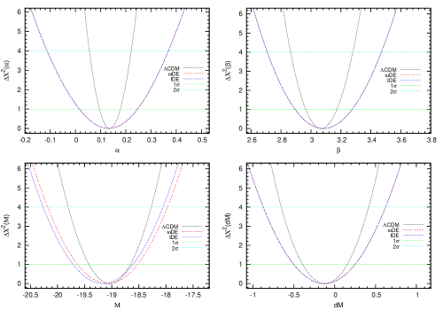
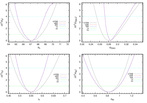
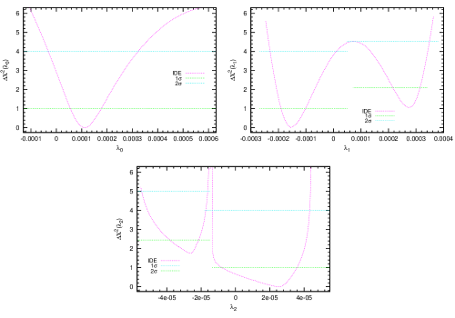
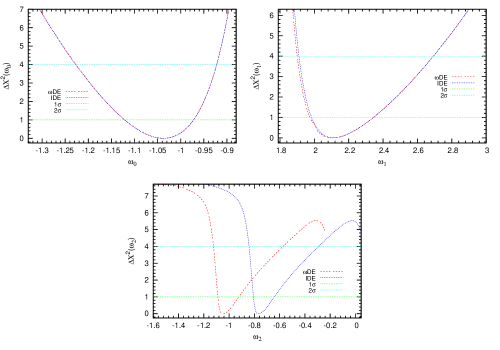
Figure 1: Displays the one-dimension probability contours of the parameter space at $1\sigma$ and $2\sigma$ errors. Besides $\mathrm{\Delta{\chi^{2}}=\chi^{2}-{\chi^{2}_{min}}}$.

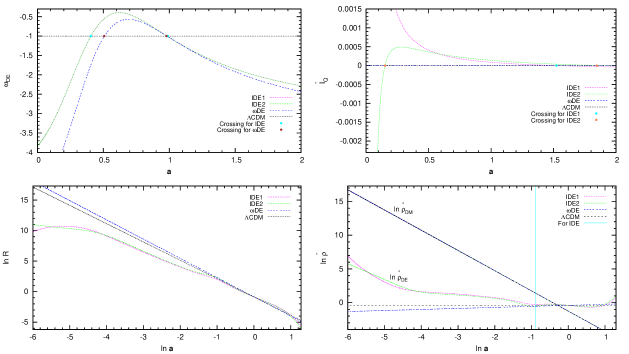
Figure 2: Shows the background evolution of $\mathrm{\omega_{DE}}$ and ${\bar{\rm I}}_{\rm Q}$, $\mathrm{R}$ and $\mathrm{\bar{\rho}}$ along $\mathrm{a}$ for the coupled and uncoupled models. Here, we have fixed the best-fit values of Table 5 and have omitted the constraints at $1\sigma$ and $2\sigma$ to have a better visualization of the results.

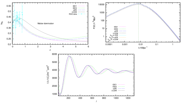
Figure 3: Shows the combined impact of $\bar{Q}$ and $\mathrm{\omega_{DE}}$ on the evolution of the structure growth of the matter $\mathrm{f\sigma_{8}}$, on the linear matter power spectrum $\mathrm{P(k)}$, and on the CMB temperature power spectrum $\it{l(l+1)C_{l}}\mathrm{(2\pi)^{-1}}\mathrm{(\mu k)^{2}}$, respectively.

The left above panel of Fig. 3, shows the evolution of the structure growth of the matter, $\mathrm{f\sigma_{8}}$, along $\mathrm{z}$ for the different cosmologies. These curves are comparable with each other at $\mathrm{z<0.4}$ but they deviate one after another at $\mathrm{z>0.4}$. It implies that they are sensitive to the background cosmology. Within the matter era the amplitude of $\mathrm{f\sigma_{8}}$ in the IDE model is enhanced relative to the $\omega$DE model at $\mathrm{z}<3$, but both are smaller than that found in the $\Lambda$CDM. At $\mathrm{z}>5$, $\bar{Q}$ and $\mathrm{\omega_{DE}}$ would brough about a large structure formation in the IDE and $\omega$DE scenarios, respectively. Due to the fact that the amount of DM is bigger than the amount of DE at earlier times; therefore, it produces an enhancement on the amplitudes of $\mathrm{f\sigma_{8}}$ in the IDE model respect to that found in the $\Lambda$CDM, respectively. Our fitting results are consistent at $1\sigma$ error with those reported by Mehrabi2015 ; Clemson2012 ; Alcaniz2013 ; Yang2014 ; Mota2017 . The right above panel of this Figure depicts the evolution of the total matter power for different scenarios at $\mathrm{z=1.6}$. Notice that $\mathrm{P(k)}$ in the IDE model is enhanced with respect to that in the $\Lambda$CDM but it is suppressed in relation to that found in the $\omega$DE scenario. That could be a consequence of the amount of concentrated matter at early times and also the presence of $\bar{Q}$. Moreover, the vertical line indicates the turnover position, $\mathrm{k_{eq}}$, is very close in our models. Also, we notice a series of wiggles on the $\mathrm{P(k)}$ due to the coupling between the photons and baryons before recombination; namely, the presence of baryons have left their effect there. these arguments, the IDE and $\omega$DE can be distinguished from the curves of $\mathrm{f\sigma_{8}}$, and the structure growth data could break the possible degeneracy between these two models and provides a signature to discriminate them. These outcomes are in correspondence with those found by Clemson2012 ; Yang2014 ; Mota2017 at $1\sigma$ error. Likewise, the below panel of this Figure displays the effects of $\bar{Q}$ and $\mathrm{\omega_{DE}}$ on the amplitude of the CMB temperature power spectrum at low multipoles $\textit{l}<100$, in where the amplitude of the integrated Sachs-Wolfe effect is deviated in the IDE model respect to that found in the other scenarios. Instead, at high multipoles ${\textit{l}>100}$, $\bar{Q}$ and $\mathrm{\omega_{DE}}$ increase the concentration of DM early times, affecting the sound horizon at the end, which shiftes to right the values of the acoustic peaks located at $\textit{l}=n_{p}\pi D_{A}(z_{*})/r_{s}(z_{*}),\,n_{p}=1,2,3..$, and reduced the amplitudes of the first peaks when the studied models are compared. These features can be understood by considering the extra-terms proportionals to $\mathrm{{\lambda}_{0}}$, $\mathrm{{\lambda}_{1}}$ and $\mathrm{{\lambda}_{2}}$ in the $\mathrm{\Omega_{DM}}$, which increases and, in consequence, amplifies the amount of DM at early times. That is in accordance with the result found in the previous panel of this Figure and with those found in Clemson2012 ; Yang2014 ; Mota2017 at $1\sigma$ error.

6 Conclusions

In this work, we examined an interacting DE model with an interaction $\bar{Q}$ proportional to the DM energy density, to the Hubble parameter $\bar{H}$, and to a time-varying function, ${\bar{\rm I}}_{\rm Q}$ expanded in terms of the Chebyshev polynomials $T_{n}$, defined in the interval $[-1,1]$. Besides, we also consider a time-varying EoS parameter, $\mathrm{\omega_{DE}}$, expressed in function of those polynomials. These ansatzes have been proposed so that their background evolution are free of divergences at the present time and also at the future time, respectively. In a Newtonian gauge and on sub-horizon scales, a set of perturbed equations is obtained when the momentum transfer potential becomes null in the DM rest-frame. This leads to different cases in the IDE model. Based on a combined analysis of geometric and dynamical probes which include JLA + RSD + BAO + CMB + H data and using the MCMC, we found the best-fit parameters that constrain the background evolution of our models.
We have also considered the perturbed equations for the DM and baryons in the rest-frame of DM. Besides, we have built the theoretical and numerical structures, and in particular, we used the c++ language to show the combined impact of both $\bar{Q}$ and $\mathrm{\omega_{DE}}$ on the evolution of $\mathrm{R}$, $\mathrm{{\bar{\rho}}_{DM}}$, $\mathrm{{\bar{\rho}}_{DE}}$, $\mathrm{f\sigma_{8}}$, $\mathrm{P(k)}$ and $\sl{l(l+1)C_{l}}$, respectively.
Likewise from Table 5 and Fig. 2, our fitting results show that ${\bar{\rm I}}_{\rm Q}$ can cross twice the line $\bar{Q}=0$ during its background evolution. Similarly, $\mathrm{\omega_{DE}}$ crosses the line $\mathrm{\omega_{DE}}=-1$ twice as well. These crossing features are favored by the data at $1\sigma$ error. Furthermore, we also notice that $\mathrm{R}$ is always positive and remains finite in all our models when $\mathrm{\bf a}\rightarrow\infty$. Moreover, in the IDE model, $\mathrm{R}$ exhibits a sca-ling behaviour at early times (keeping constant). Then, $\bar{Q}$ seems to alleviate the coincidence problem for ln $\mathrm{\bf a}\leq 0$ but it does not solve that problem in full.
On the other hand, from Fig. 3, we found that the evolution curve of $\mathrm{f\sigma_{8}}$ in the IDE model deviates significantly from that obtained in the $\Lambda$CDM and $\omega$DE models. It meant that, the structure formation data could break the possible degenaracy between the IDE and $\omega$DE models. In these last two models, several best-fit parameters are very close with each other, therefore, one could then conclude that this detected deviation is brough about mainly by $\mathrm{\omega_{DE}}$, namely, $\mathrm{f\sigma_{8}}$ is sensitive mainly to the evolution of $\mathrm{\omega_{DE}}$ and depends on its parametrisation. Moreover, the geometric probes favor the existence of an interaction between the dark sectors but the dynamical test constrains its intensity. These effects can be understood by conside-ring the extra-terms proportional to ${\bar{\rm I}}_{\rm Q}$ in the DM ener-gy density, (see Eq. (12)), which increases and, in consequence, amplifies the amount of DM at earlier times. As a result, the growth of structure is significantly affec-ted by $\bar{Q}$ and $\mathrm{\omega_{DE}}$, which induce that the amplitude of $\mathrm{P(k)}$ becomes higher in the IDE model than that found in the $\Lambda$CDM model but it is lesser than that found in the $\omega$DE. Moreover, the position of the turnover point in all our models is very close at smaller scales. Likewise, we also notice a series of wiggles on the curve of $\mathrm{P(k)}$ due to the coupling between the photons and baryons before of the recombination; namely, the presence of baryons have left their effect in this plot (see Fig. 3). Finally, we also find that the amplitude of the CMB temperature power spectrum is also sensitive to $\bar{Q}$ at low and high multipoles. In the IDE model, $\bar{Q}$ produces a shift of the acoustic peaks to the right and their amplitudes are reduced at high multipoles with respect to the uncoupled models. Besides, at low multipoles the amplitude of the integrated Sachs-Wolfe effect is also affected by $\bar{Q}$.
The results for the other case when the momentum-transfer potential vanishing in the DE rest-frame will be presented in a future work.

Acknowledgments
The author is indebted to the Instituto de Física y Matemáticas (UMSNH) for its hospitality and support.

References

• (1) Conley A et al., Astrophys. J. Suppl. 192 (2011) 1.
• (2) Jönsson, J., et al. 2010, Mon. Not. Roy. Astron. Soc. 405 (2010) 535.
• (3) Betoule M et al., Astron. and Astrophys. 568 (2014) A22.
• (4) J. C. Jackson, Mon. Not. Roy. Astron. Soc. 156 (1972) 1P.
• (5) Kaiser N., Mon. Not. Roy. Astron. Soc. 227 (1987) 1.
• (6) A. Mehrabi, S. Basilakos, F. Pace, Mon. Not. Roy. Astron. Soc. 452 (2015) 2930-2939.
• (7) Alcock C. and Paczynski B., Nature. 281 (1979) 358.
• (8) H-J. Seo, E. R. Siegel, D. J. Eisenstein, and M. White, Astrophys. J. 686 (2008) 13Y24.
• (9) R. A. Battye, T. Charnock and A. Moss Phys. Rev. D 91 (2015) 103508.
• (10) L. Samushia, et al., Mon. Not. Roy. Astron. Soc. 439 (2014) 3504.
• (11) Hudson M. J., Turnbull S. J., Astrophys. J. 751 (2013) L30.
• (12) Beutler F., Blake C., Colless M., Jones D. H., Staveley-Smith L., et al., Mon. Not. Roy. Astron. Soc. 423 (2012) 3430.
• (13) Feix M., Nusser A., Branchini E., Phys. Rev. Lett. 115 (2015) 011301.
• (14) Percival W. J., et al., Mon. Not. Roy. Astron. Soc. 353 (2004) 1201.
• (15) Y-S. Song and W. J. Percival, J. Cosmol. Astropart. Phys. 10 (2009) 004.
• (16) Tegmark M. et al., Phys. Rev. D 74 (2006) 123507.
• (17) Guzzo L. et al., Nature. 451 (2008) 541.
• (18) Samushia L., Percival W. J., Raccanelli A., Mon. Not. Roy. Astron. Soc. 420 (2012) 2102.
• (19) Blake C. et al., Mon. Not. Roy. Astron. Soc. 415 (2011) 2876; Mon. Not. Roy. Astron. Soc. 418 (2011) 1725.
• (20) Tojeiro R., Percival W., Brinkmann J., Brownstein J., Eisenstein D., et al., Mon. Not. Roy. Astron. Soc. 424 (2012) 2339.
• (21) Reid B. A., Samushia L., White M., Percival W. J., Manera M., et al., Mon. Not. Roy. Astron. Soc. 426 (2012) 2719.
• (22) de la Torre S., Guzzo L., Peacock J., Branchini E., Iovino A., et al., Astron. Astrophys. 557 (2013) A54.
• (23) Planck 2015 results, XIII. Cosmological parameters, Astron. Astrophys. 594 (2016) A13.
• (24) WMAP collaboration, G. Hinshaw et al., Astrophys. J. Suppl. 208 (2013) 19.
• (25) F. Beutler et al., Mon. Not. Roy. Astron. Soc. 416 (2011) 3017.
• (26) A. J. Ross et al., Mon. Not. Roy. Astron. Soc. 449 (2015) 835.
• (27) W. J. Percival et al., Mon. Not. Roy. Astron. Soc. 401 (2010) 2148.
• (28) E. A. Kazin et al., Astrophys. J. 710 (2010) 1444.
• (29) N. Padmanabhan et al., Mon. Not. Roy. Astron. Soc. 427 (2012) 2132.
• (30) C. H. Chuang and Y. Wang, Mon. Not. Roy. Astron. Soc. 435 (2013) 255.
• (31) C-H. Chuang and Y. Wang, Mon. Not. Roy. Astron. Soc. 433 (2013) 3559.
• (32) L. Anderson et al., Mon. Not. Roy. Astron. Soc. 441 (2014) 24.
• (33) E. A. Kazin et al., Mon. Not. Roy. Astron. Soc. 441 (2014) 3524.
• (34) T. Delubac et al., Astron. Astrophys. 574 (2015) A59.
• (35) A. Font-Ribera et al., J. Cosmol. Astropart. Phys. 05 (2014) 027.
• (36) D. J. Eisenstein, W. Hu, Astrophys. J. 496 (1998) 605.
• (37) D. J. Eisenstein et al., Astrophys. J. 633 (2005) 560.
• (38) M. D. P. Hemantha, Y. Wang and C-H. Chuang., Mon. Not. Roy. Astron. Soc. 445 (2014) 3737.
• (39) J. R. Bond, G. Efstathiou and M. Tegmark, Mon. Not. Roy. Astron. Soc. 291 (1997) L33.
• (40) W. Hu and N. Sugiyama, Astrophys. J. 471 (1996) 542.
• (41) J. Neveu, V. Ruhlmann-Kleider, P. Astier, M. Besançon, J. Guy, A. Möller, E. Babichev, Astron. and Astrophys. 600 (2017) A40.
• (42) G. S. Sharov, J. Cosmol. Astropart. Phys. 06 (2016) 023.
• (43) C. Zhang et al., Res. Astron. Astrophys. 14 (2014) 1221.
• (44) J. Simon, L. Verde and R. Jimenez, Phys. Rev. D 71 (2005) 123001.
• (45) M. Moresco et al., J. Cosmol. Astropart. Phys. 8 (2012) 006.
• (46) E. Gastañaga, A. Cabre, L. Hui, Mon. Not. Roy. Astron. Soc. 399 (2009) 1663.
• (47) A. Oka et al., Mon. Not. Roy. Astron. Soc. 439 (2014) 2515.
• (48) C. Blake et al., Mon. Not. Roy. Astron. Soc. 425 (2012) 405.
• (49) D. Stern, R. Jimenez, L. Verde, M. Kamionkowski and S. A. Stanford, J. Cosmol. Astropart. Phys. 02 (2010) 008.
• (50) M. Moresco, Mon. Not. Roy. Astron. Soc. 450 (2015) L16-L20.
• (51) N. G. Busca et al., Astron. Astrophys. 552 (2013) A96.
• (52) V. Sahni, Lect. Notes Phys. 653 (2004) 141; E. J. Copeland, M. Sami and S. Tsujikawa, Int. J. Mod. Phys. D 15 (2006) 1753.
• (53) U. Seljak, et al., Phys. Rev. D 71 (2005) 103515; M. R. Garousi, M. Sami, and S. Tsujikawa, Phys. Rev. D 71 (2005) 083005. M. K. Mak and T. Harko, Phys. Rev. D 71 (2005) 104022; X. Cheng, Y. Gong and E. N. Saridakis, J. Cosmol. Astropart. Phys. 04 (2009) 001; E. Rozo et al., Astrophys. J. 708 (2010) 645;
• (54) Z. K. Guo, N. Ohta, and S. Tsujikawa, Phys. Rev. D 76 (2007) 023508; J. H. He and B. Wang, J. Cosmol. Astropart. Phys. 06 (2008) 010; S. Campo, R. Herrera and D. Pavón, J. Cosmol. Astropart. Phys. 01 (2009) 020; S. Cao, N. Liang and Z. H. Zhu, Int. J. Mod. Phys. D 22 (2013) 1350082.
• (55) G. Olivares, F. Atrio-Barandela, and D. Pavón, Phys. Rev. D 71 (2005) 063523.
• (56) D. Pavón, B. Wang, Gen.Rel.Grav. 41 (2009) 1-5; S. del Campo, R. Herrera, G. Olivares, and D. Pavón, Phys. Rev. D 74 (2006) 023501.
• (57) B. Wang, C. Y. Lin and E. Abdalla, Phys. Lett. B 637 (2006) 357.
• (58) F. Cueva Solano and U. Nucamendi, J. Cosmol. Astropart. Phys. 04 (2012) 011; F. Cueva Solano and U. Nucamendi, arXiv: 1207.0250 07 (2012) 02.
• (59) J. Valiviita, E. Majerotto and R. Maartens, J. Cosmol. Astropart. Phys. 07 (2008) 020.
• (60) T. Clemson, K. Koyama, G. B. Zhao, R. Maartens and J. Valiviita Phys. Rev. D 85 (2012) 043007.
• (61) S. Tsujikawa, A. De Felice and J. Alcaniz, J. Cosmol. Astropart. Phys. 01 (2013) 030.
• (62) W. Yang and L. Xu, Phys. Rev. D 89 (2014) 083517.
• (63) W. Yang, S. Pan, and D. F. Mota, Phys. Rev. D 96 (2017) 123508.
• (64) M. Chevallier, D. Polarski, Int. J. Mod. Phys. D 10 (2001) 213; E. V. Linder, Phys. Rev. Lett. 90 (2003) 091301.
• (65) H. Li and X. Zhang, Phys. Lett. B 703 (2011) 119; J. Z. Ma and X. Zhang, Phys. Lett. B 699 (2011) 233.
• (66) E. F. Martinez and L. Verde, J. Cosmol. Astropart. Phys. 08 (2008) 023.
• (67) S. del Campo, R. Herrera, and D. Pavón Phys. Rev. D 91 (2015) 123539;
• (68) L. P. Chimento, A. S. Jakubi, D. Pavón, and W. Zimdahl, Phys. Rev. D 67 (2003) 083513; J. Q. Xia and M. Viel, J. Cosmol. Astropart. Phys. 04 (2009) 002.
• (69) D. J. Eisenstein and W. Hu, Astrophys. J. 496 (1998) 605.
• (70) S. Dodelson, Modern Cosmology. Academic Press, Elsevier Science, (2003).
• (71) Limber D., 1953, The Astrophysical Journal, 117, 134
• (72) S. Nesseris and L. Perivolaropoulos, J. Cosmol. Astropart. Phys. 01 (2007) 018.
• (73) R. G. Cai and Q. Su, Phys. Rev. D 81 (2010) 103514.
• (74) Y. H. Li and X. Zhang, Eur. Phys. J. C. 71 (2011) 1700.