Damping Effect on PageRank Distribution

Abstract

This work extends the personalized PageRank model invented by Brin and Page to a family of PageRank models with various damping schemes. The goal with increased model variety is to capture or recognize a larger number of types of network activities, phenomenons and propagation patterns. The response in PageRank distribution to variation in damping mechanism is then characterized analytically, and further estimated quantitatively on $6$ large real-world link graphs. The study leads to new observation and empirical findings. It is found that the difference in the pattern of PageRank vector responding to parameter variation by each model among the $6$ graphs is relatively smaller than the difference among $3$ particular models used in the study on each of the graphs. This suggests the utility of model variety for differentiating network activities and propagation patterns. The quantitative analysis of the damping mechanisms over multiple damping models and parameters is facilitated by a highly efficient algorithm, which calculates all PageRank vectors at once via a commonly shared, spectrally invariant subspace. The spectral space is found to be of low dimension for each of the real-world graphs.

I Introduction

Personalized PageRank, invented by Brin and Page [1, 2], revolutionized the way we model any particular type of activities on a large information network. It is also intended to be used as a mechanism to counteract malicious manipulation of the network [1, 2, 3]. PageRank has underlain Google’s search architecture, algorithms, adaptation strategies and ranked page listing upon query. It has influenced the development of other search engines and recommendation systems, such as topic-sensitive PageRank[4]. Its impact reaches far beyond digital and social networks. For example, GeneRank is used for generating prioritized gene lists[5, 6]. The seminal paper [1] itself is directly cited more than ten thousands times as of today. As surveyed in [7, 8], a lot of efforts were made to accelerate the calculation of personalized PageRank vectors, in part or in whole [9, 10]. Certain investigation were carried out to assess the variation in PageRank vector in response to varying damping parameter [11, 12]. Most efforts on PageRank study, however, are ad hoc to the Brin-Page model. Chung made a departure by introducing a diffusion-based PageRank model and applied it to graph cuts [13, 14].

In this paper we follow Brin and Page in the modeling aspect that warrants more attention as the variety of networks and activities on the networks increases incessantly. We extend the model scope to capture more network activities in a probabilistic sense. We study the damping effect on PageRank distribution. We consider the holistic distribution because it serves as the statistical reference for inferring conditional page ranking upon query. Our study has three intellectual merits with practical impact. (1) A family of damping models, which includes and connects the Brin-Page model and Chung’s model. The family admits more probabilistic descriptions of network activities. (2) A unified analysis of damping effect on personalized PageRank distribution, with parameter variation in each model and comparison across models. The analysis provides a new insight into the solution space and solution methods. (3) A highly efficient method for calculating the solutions to all models under consideration at once, particular to a network and a personalized vector. Our quantitative analysis of $6$ real-world network graphs leads to new findings about the models and networks under study, which we present and discuss in Sections III and V. Our modeling and analysis methods can be potentially used for recognizing and estimating activity or propagation patterns on a network, provided with monitored data.

II PageRank models

We first review briefly two precursor models and then introduce a family of PageRank models.

II-A Brin-Page model

Brin and Page describe a network of webpages as a link graph, which is represented by a stochastic matrix $P$ [1]. We adopt the convention that $P$ is stochastic columnwise. Every webpage is a node with (outgoing) links, i.e., edges, to some other webpages and with incoming edges or backlinks as citations to the page. If page $j$ has $n_{j}>0$ outgoing links, then in column $j$ of $P$, $P_{i,j}=1/n_{j}$ if page $j$ has a link to page $i$; $P_{i,j}=0$, otherwise. In row $i$ of $P$, every nonzero element $P_{i,j}$ corresponds to a backlink from $j$ to $i$. In the Brin-Page model, the web user behavior is described as a random walk on a personalized Markov chain (i.e., a discrete-time Markov chain) associated with the following probability transition matrix

$$M_{\alpha}(v)=\alpha P+(1-\alpha)ve^{\rm T},\quad\alpha\in(0,1),\quad e^{\rm T}v=1,$$ (1)

where $v\geq 0$ is a personalized or customized distribution/vector, $e$ denotes the vector with all elements equal to $1$, and the damping factor $\alpha$ describes a Bernoulli decision process. At each step, with probability $\alpha$, the web user follows an outlink; or with probability $(1-\alpha)$, the user jumps to any page by the personalized distribution $v$. The personalized transportation term is innovative. It customizes the Markov chain with respect to a particular type of relevance. In this paper we assume that the personalized vector $v$ is given and fixed, and focus on investigating the damping effect. In particular, with Brin-Page model, we focus on the role of $\alpha$. The notation for the Markov chain may thus be simplified to $M_{\alpha}$, or $M$ when $\alpha$ is clear from the context.

Page ranking upon a search query depends on the stationary PageRank distribution, denoted by $x=x(\alpha)$, of the Markov chain:

$$M_{\alpha}\,x=x,\quad e^{\rm T}x=1.$$ (2)

Arasu et al[15] recast the eigenvector equation (2) to a linear system to solve for $x$,

$$(I-\alpha P)x=(1-\alpha)v,$$ (3)

where $I$ is the identity matrix. Because $\alpha\|P\|_{1}<1$, the solution can be expressed via the Neumann series for the inverse of $(I-\alpha P)$,

$$x(\alpha)=(1-\alpha)\sum_{k=0}^{\infty}\alpha^{k}P^{k}v.$$ (4)

The weights $(1-\alpha)\alpha^{k}$ decrease by the factor $\alpha$ from one step to the next. In [1], Brin and Page set $\alpha$ to $0.85$.

In (4), the solution to Brin-Page model with $\alpha\in(0,1)$ is not the stationary distribution of network $P$. It is analyzed in terms of steps on $P$. Term $k$ represents the probabilistic accumulation of the Bernoulli decision process at each step by (1) to step $k$, $k\geq 0$. Every step has its print in distribution $x(\alpha)$.

II-B Chung’s model

Chung introduced a PageRank model [13] in the form of a heat or diffusion equation, with $v$ as the initial distribution,

$$\frac{\partial x}{\partial\beta}=-(I-P)x,\quad x(0)=v,$$ (5)

where $(I-P)$ is the Laplacian of the link graph, and we use $\beta$ to denote the time variable. From the viewpoint of probabilistic theory, model (5) is underlined by the Kolmogorov’s backward equation system for a continuous-time Markov chain with $-(I-P)$ as the transition rate matrix and with the identity matrix $I$ as the initial transition matrix. The solution to (5) is

$$x(\beta)=e^{-\beta(I-P)}v=e^{-\beta}\sum_{k=0}^{\infty}\frac{\beta^{k}}{k!}P^{k}v.$$ (6)

II-C A model family

We introduce a family of PageRank models. Each member model is characterized by a scalar damping variable $\rho$ and a discrete probability mass function (pmf) $w(\rho)=\{w_{k}=w_{k}(\rho),\ k\in\mathbb{N}_{w}\}$. The support $\mathbb{N}_{w}\subset\mathbb{N}$ may be finite or infinite. There are a few equivalent expressions to describe our models. We start by defining the model with a kernel function $f(\lambda,\rho)$,

$$f(\lambda,\rho)=\sum_{k\in N_{w}}w_{k}(\rho)\,\lambda^{k},\quad|\lambda|\leq 1.$$ (7)

The solution specific to network graph $P$ and personalized vector $v$ is,

$$x_{f}(\rho)=f(P)v=\mathopen{}\mathclose{{}\left(\sum_{k\in N_{w}}w_{k}(\rho)\,P^{k}}\right)v.$$ (8)

The matrix function $f(P)$ is stochastic. The rank distribution vector $x_{f}$ is the superposition of step terms with probabilistic weights $w_{k}$. The step term $k$ describes the probabilistic propagation of $v$ at step $k$. For a specific case, the damping variable may have a designated label, with a specific range, and the pmf may have a specific support and additional parameters. For convenience, we assume $\mathbb{N}$ as the support. Over the infinite support, the damping weights must decay after certain number of steps and vanish as $k$ goes to infinity. In theory, every discrete pmf can be used as a model kernel in (8). In practice, each describes a particular type of activity or propagation.

The family includes Brin-Page model and Chung’s model. For the former, the damping variable is denoted by $\alpha$, the damping weights $(1-\alpha)\alpha^{k}$, $k\geq 0$, follow the geometric distribution with the expected value $\alpha(1-\alpha)^{-1}$. The kernel function is $(1-\alpha)(1-\alpha\lambda)^{-1}$. For Chung’s model, we denote the damping variable by $\beta$, $\beta>0$. The damping weights $e^{-\beta}\beta^{k}/k!$, $k\geq 0$, follow the Poisson distribution with the expected value $\beta$. The model’s kernel function is $e^{-\beta(1-\lambda)}$.

We describe a few other models, among many, in the family. In fact, the precursor models are two special cases of the model associated with the Conway-Maxwell-Poisson (CMP) distribution, which has an additional parameter $\nu$ to the pmf,

$$w_{k}(\rho,\nu)=\frac{\rho^{k}}{(k!)^{\nu}\,Z},\quad\nu>0,$$

where $Z$ is the normalization scalar, and $\nu$ is the decay rate parameter. The case with $\nu=0$ is the geometric distribution; the case with $\nu=1$ is the Poisson distribution. If the value of $\rho$ is fixed, the weights decay faster with a larger value of $\nu$. The negative binomial distribution, or the Pascal distribution, also includes the geometric distribution as a special case. It includes other cases that render damping weights with slower decay rates.

In the rest of the paper, for the purpose of including and illustrating new models, we use the model associated with the logarithmic distribution, for $\gamma\in(0,1)$,

$$f(\lambda,\gamma)=\frac{-1}{\ln(1-\gamma)}\sum_{k=1}^{\infty}\frac{(\gamma\lambda)^{k}}{k}=\frac{\ln(1-\gamma\lambda)}{\ln(1-\gamma)}.$$ (9)

The weights decrease slightly faster than the geometrically distributed ones, but not in the CMP distribution class.

We now present the system of linear equations with $x(\rho)$ in (8) as the solution,

$$A(P)x=v,\quad A(P)=f^{-1}(P).$$ (10)

The matrix $A$ is an $M$ matrix. In particular, $A=(1-\alpha)^{-1}(I-\alpha P)$ for Brin-Page model, $A=e^{\beta(I-P)}$ for Chung’s model and $A=\ln(1-\gamma)\,\ln^{-1}(I-\gamma P)$ for the log-$\gamma$ model (9). The algebraic model expression (10) will be used next for the model expression in a differential equation.

III Response to variation in damping

We provide a unified analysis of the response in PageRank distribution to the variation in the damping parameter value as well as to the change, or connection, from one model to another.

III-A Intra-model damping variation

By (8), we obtain the trajectory of the PageRank vector $x(\rho)$ with the change in the damping variable $\rho$,

$$\dot{x}(\rho)=\frac{dx(\rho)}{d\rho}=\frac{\partial}{\partial\rho}f(P)v=Q(P)\,x(\rho),$$ (11)

where $Q(P)=\frac{\partial}{\partial\rho}f(P)f^{-1}(P)$ by (10), which we may refer to as the $\rho$-transition matrix. Equation (11) generalizes Chung’s diffusion model (5), in which the $\beta$-transition matrix $Q=-(I-P)$ is independent of $\beta$. For the Brin-Page model with damping variable $\alpha$,

$$Q(\alpha)=\mathopen{}\mathclose{{}\left[P(I-\alpha P)^{-1}-(1-\alpha)^{-1}I}\right].$$ (12)

For the log-$\gamma$ model (9),

$$Q(\gamma)=\frac{(1-\gamma)^{-1}}{\ln(1-\gamma)}I-P(I-\gamma P)^{-1}(\ln(I-\gamma P))^{-1}.$$ (13)

For each model, $e^{\rm T}Q=0$.

In addition to the element-wise response in the rank vector, we would also like to have an aggregated measure of the response to variation in $\rho$. Let $x(\rho_{o})$ be a reference PageRank vector. We may use Kullback-Leibler divergence [16] to measure the discrepancy of $x(\rho)$ from $x(\rho_{o})$,

$$KL(x(\rho),x(\rho_{o}))=\sum_{i}x_{i}(\rho)\log{\frac{x_{i}(\rho)}{x_{i}(\rho_{o})}}.$$ (14)

When $\rho=\rho_{o}$, $KL(x(\rho),x(\rho_{o}))=0$. We have the rate of change in KL divergence with the variation in $\rho$,

$$\frac{d}{d\rho}KL(x(\rho),x(\rho_{o}))=\dot{x}(\rho)^{\rm T}\mathopen{}\mathclose{{}\left(\log{x(\rho)}-\log{x(\rho_{o})}+e}\right)$$ (15)

We will describe in Section IV efficient algorithms for calculating the vectors and measures above.

III-B Inter-model correspondence

Each model has its own damping form and parameter. The expected value of the step weight distribution is,

$$\mu(w(\rho))=\sum_{k\in\mathbb{N}_{w}}k\cdot w_{k}(\rho).$$ (16)

We may explain this as the expected value of walking steps. We establish the point of correspondence between models by their expected values. That is, for any two models, we set their expected values equal to each other. Without loss of generality, we let the expected values for the Brin-Page model serve as the reference. In particular, we have the correspondence equalities

$$\frac{\alpha}{1-\alpha}=\beta,\quad\frac{\alpha}{1-\alpha}=\mathopen{}\mathclose{{}\left(\frac{\gamma}{1-\gamma}}\right)\frac{-1}{\ln(1-\gamma)}$$ (17)

for Chung’s model and for the log-$\gamma$ model, respectively. We will show the comparisons in PageRank vectors at such correspondence points in Section V.

IV Efficient algorithms for batch ranking

We introduce novel algorithms for efficient quantitative analysis of damping effect on PageRank distribution. Provided with a network graph $P$ and a personalized distribution vector $v$, the algorithms can be used in one batch of computation across multiple models as well as over a range of damping parameter value per model.

IV-A Reduction to irreducible subnetworks

Information networks in real world applications are not necessarily irreducible and aperiodic as assumed by many existing iterative solutions for guaranteed convergence. To meet such convergence conditions, some heuristics were used to perturb or twist the network structure with artificially introduced links [17, 18]. Instead, we decompose the network into strongly connected sub-networks by applying the Dulmage-Mendelsohn (DM) decomposition algorithm [19] to the Laplacian matrix $I-P$. The DM algorithm is highly efficient when diagonal elements are non-zero. It renders the matrix in block upper triangular form. See Figure 1 for the Google link graph released by Google in 2002 [20]. Each diagonal block $B_{ii}$ corresponds to a subnetwork. A square diagonal block corresponds to an irreducible subnetwork. A non-zero off-diagonal block $B_{ij}$ in the upper part, $i<j$, represents the links from cluster $j$ to cluster $i$. The top block is associated with a sink cluster without outgoing links to other cluster; the bottom block is associated with a source cluster without incoming edges from other clusters. The solution for the entire network can be obtained by the solutions to the subnetworks and successive back substitution.

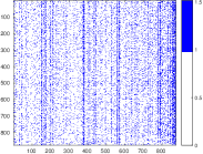
((a)) original link graph

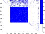
((b)) link graph after DM permutation

Figure 1: The 1:1000 sparsity map of adjacency matrix of Google link graph [20] with 875,713 page nodes in (a) the provided ordering and (b) the ordering rendered by the DM decomposition, depicted by imagesc in matlab. Each point shows the number of non-zeros, in log scale, in the corresponding $1000\times 1000$ block. The subnetwork in the middle of (b) is strongly connected with 434,818 nodes.

IV-B Cascade of iterations

Several iterative methods exist for computing the PageRank vector by the Brin-Page model. They include the power method by the eigenvector equation (2), and the Jacobi, Gauss-Seidel, and SOR methods by equation (3). There are various acceleration techniques used for calculating the PageRank vector, or a small part of the vector, or even a single pair of nodes between the personalized vector and the PageRank vector [21, 10, 22, 23]. For the Brin-Page model, the iterative methods converge slower as $\alpha$ increases and gets closer to $1$. We developed a cascading initialization scheme. The solution to the model with $\alpha$ is used as the initial guess to the iteration for the solution to the model with $\alpha+\delta\alpha$, $\delta\alpha>0$. Although it has accelerated the computation with successively increased $\alpha$ values, this technique is limited to sequential computation and ad hoc to the Brin-Page model. We introduce next a novel algorithm without these limitations.

IV-C Shared invariant Krylov space

Our new algorithm for batch calculation of PageRank vectors with multiple models and parameter values is based on the very fact that the solutions to the models in Section II all reside in the same Krylov space,

$${\cal K}(P,v)=\{v,Pv,P^{2}v,\cdots,P^{k}v,\cdots\},\quad\begin{array}[]{l}v\geq 0\\ e^{\rm T}v=1\end{array}.$$ (18)

The space has the property $P{\cal K}(P,v)={\cal K}(P,v)$, i.e., it is a spectrally invariant subspace. In PageRank terminology, ${\cal K}(P,v)$ is a personalized invariant subspace. We have the remarkable fact about the model family in Section II.

Theorem 1.

Any model solution (8), at any particular damping parameter value, and its trajectory (11) are functions in the Krylov space ${\cal K}(P,v)$.

Theorem 2.

Let $m=\mbox{dimension}({\cal K})$. Denote by $K$ the matrix composed of the Krylov vectors. Let $K=QR$ be the QR factorization of $K$. Then, $Qe_{1}=v$ and $PQ=QH$, where $H$ is an $m\times m$ upper Hessenberg matrix, and $e_{1}$ is the first column of the identity matrix $I$.

A few remarks. Matrix $H$ in Theorem 2 is the representation of matrix $P$ under basis $Q$ in the Krylov space. In numerical computation, we use a rank-revealing version of the QR factorization with $Qe_{1}=v$. In theory, the dimension $m$ is equal to the number of spectrally invariant components of $P$ that present in $v$. In the extreme case, $m=1$ when $v$ is the Perron vector of $P$. In general, by the condition $e^{\rm T}v=1$, $v$ is not deficient in Perror component. In our study on real-world graphs, which we will detail shortly in Section V, the numerical dimension is low, matrix $H$ is therefore small. We may view this as a manifest of the smallness of the real-world graphs under study. We exploit these theoretical and practical facts.

Corollary 3.

For any function $g$ in the Krylov space (18), we have $g(P)v=Qg(H)e_{1}$.

When dimension $m$ is modest, we translate by Corollary 3 the calculation of $x_{g}=g(P)v$ with $N\times N$ matrix $P$ on vectors to the calculation of $\hat{x}_{g}=g(H)e_{1}$ with $m\times m$ matrix $H$ on vectors, followed by a matrix-vector product $Q\hat{x}_{g}$. The vector $\hat{x}_{g}$ is the spectral representation of $x_{g}$ in the Krylov space. In the model family, solutions $x_{f}$ (8) differ from one to another in their spectral representations $\hat{x}_{f}$, they share the same basis matrix $Q$ in the ambient network space.

Our algorithm consists of the following major steps. Let ${\cal G}=\{g\}$ be a set of functions under study. (1) Calculuate Krylov vectors to form matrix $K$ in Theorem 2, apply rank-revealing $QR$ factorization to $K$, and find numerical dimension $m$; (2) Construct the matrix $H$, by Theorem 2, from $R$ and the permutation matrix $\Pi$ rendered by the rank-revealing $QR$; (3) Calculate $\hat{x}_{f}=g(H)e_{1}$ for all functions in ${\cal G}$; (4) Transform $\hat{x}_{f}$ from the Krylov-spectral space to the ambient network space by the same basis matrix $Q$, based on Corollary 3.

V Experiments on real-world link graphs

We show in numerical values how PageRank vector responses to variation in damping variable with each model and across models, on $6$ real-world link graphs.

V-A Experiment setup: data and models

The $6$ link graphs we used for our experiments are publicly available at the Koblenz Network Collection[24]. The basic information of the graphs is summarized in Table 1, where $\max(d_{out})$ is the maximum out-degree (the number of citations) of graph nodes, $\max(d_{in})$ is the maximum in-degree (the number of backlinks), $\mu(d_{out})=\mu(d_{in})$ is the average out-degree, which equals to the average in-degree, and LSCC stands for the largest strongly connected component(s) of the graph. The Google graph of today is reportedly containing hundreds of trillions of nodes, substantially larger than the snapshot size used here.

TABLE 1: Dataset Description

Total #nodes #nodes in LSCC $\mathopen{}\mathclose{{}\left[\max(d_{out}),\mu(d_{out}),\max(d_{in})}\right]$ Google [20] 875,713 434,818 $[4209,8.86,382]$ Wikilink [24] 12,150,976 7,283,915 $[7527,50.48,920207]$ DBpedia [25] 18,268,992 3,796,073 $[8104,26.76,414924]$ Twitter(www)[26] 41,652,230 33,479,734 $[2936232,42.65,768552]$ Twitter(mpi)[27] 52,579,682 40,012,384 $[778191,47.57,3438929]$ friendster[28] 68,349,466 48,928,140 $[3124,32.76,3124]$

For variation analysis of each graph in Table 1, the associated link matrix $P$ is well specified. We use the same personalized or customized distribution vector $v$, which we get by drawing elements from standard Gaussian distribution ${\cal N}(0,1)$, followed by normalization $v^{\rm T}e=1$. We report variation analysis results with three particular models : Brin-Page model (3) with damping variable $\alpha$, Chung’s model (5) with variable $\beta$, and the log-$\gamma$ model (9). The last is used as an illustration of new models in the family (8).

V-B Variation in PageRank vector

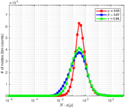
((a)) $x(\rho)$ of Google link graph

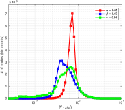
((b)) $x(\rho)$ of Twitter(www) link graph

Figure 2: Inter-model comparison of histograms of $N\cdot x_{f}(\rho)$ among the three models with corresponding parameter values $\alpha_{o}$, $\beta_{o}$ and $\gamma_{o}$ so that the expected value of walking steps for each model is $\alpha_{o}/(1-\alpha_{o})=5.\dot{6}$ with $\alpha_{o}=0.85$, see the model correspondence equalities (17). (a) comparison on Google link graph; (b) comparison on Twitter(www) link graph.

In order to show the quantitative response in PageRank vector $x_{f}$ over $N$ nodes with the variation in damping variable $\rho$, we display the histogram of $N\cdot x_{f}(\rho)$ for model $f$ at parameter value $\rho$. In Figure 2 we show the histograms associated with three models on Google network. The parameter for Brin-Page model is set to the value $\alpha_{o}=0.85$. The parameter for the other two models are set by (17). We observe that the histogram with Brin-Page model has higher and narrower peaks than Chung’s model. The histogram of log-$\gamma$ model is in between. This is expected by the relationships in the damping weights among the three models, as discussed in Section III-B.

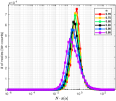
((a)) Brin-Page model

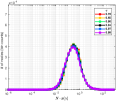
((b)) log-$\gamma$ model

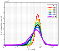
((c)) Chung’s model

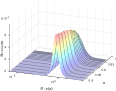
((d)) Brin-Page model

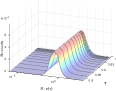
((e)) log-$\gamma$ model

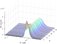
((f)) Chung’s model

Figure 3: Comparison in histograms of $N\cdot x_{f}(\rho)$ on the Google link graph over a range of damping variable value. Left column: Brin-Page model, Middle column: log-$\gamma$ model, Right column: Chung’s model. Top row: 2D display of 6 histograms associated with 6 parameter values shown in the respective legends. The histogram in black with Brin-Page model is associated with the value $\alpha=0.85$. The corresponding parameter values with Chung’s model and log-$\gamma$ model are set by (17), the associated histograms are color coded by the corresponding parameter values. Bottom row: a stack of multiple histograms shown in 3D space over the range $\alpha\in[0.7,0.97]$ with Brin-Page model, $\beta\in[2.\dot{6},32.\dot{3}]$ with Chung’s model, and $\gamma\in[0.7787,0.994]$ with log-$\gamma$ model. The histograms with Chung’s model have flattened peaks at larger values (toward the back end). The log-$\gamma$ model is nearly insensitive to $\gamma$ change in the range above.

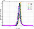
((a)) Brin-Page model

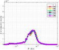
((b)) log-$\gamma$ model

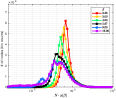
((c)) Chung’s model

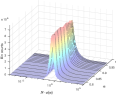
((d)) Brin-Page model

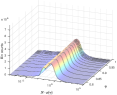
((e)) log-$\gamma$ model

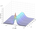
((f)) Chung’s model

Figure 4: Comparison in histogram of $N\cdot x_{f}(\rho)$ on the Twitter graph over a range of dampling value, in the same settings as in Figure 3.

Figure 3 and Figure 4 show the variation in the histograms over a range of the damping variable per model as well as the comparison side by side between the three models on two datasets. The models have similar behaviors on the other $4$ graphs in Table 1. Supplementary material can be found in [29]. With larger damping factors in the models, the distribution become less centralized. Log-$\gamma$ model, specifically, is less sensitive to $\gamma(\alpha)$ range with $\alpha\in[0.7,0.97]$.

V-C Relative variation measured by KL divergence

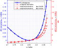
((a)) $\alpha_{o}=0.85$

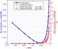
((b)) $\gamma_{o}=0.94146$

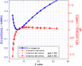
((c)) $\beta_{o}=5.\dot{6}$

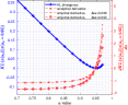
((d)) $\alpha_{o}=0.95$

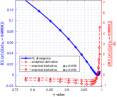
((e)) $\gamma_{o}=0.98831$

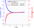
((f)) $\beta_{o}=19$

Figure 5: Intra-model relative variation as defined in (14) in PgeRank distribution, on the Google graph, with respect to two reference distribution at $\alpha_{o}\in\{0.85,0.95\}$ with Brin-Page model (left column), $\gamma_{o}\in\{0.94146,0.98831\}$ with log-$\gamma$ model (middle column), and $\beta_{o}\in\{5.\dot{6},19\}$ with Chung’s model (right column). Blue curves: the KL score $KL(x_{f}(\rho)||x_{f}(\rho_{o}))$ with numerically computed distribution vectors; Red curves: the derivative of the KL score $(d/d\rho)KL(x_{f}(\rho)||x_{f}(\rho_{o}))$. The red curves with $\cdot$ marker and $\diamond$ marker are obtained empirically from numerical distribution vectors, with step size $\Delta\rho=(0.002,0.008)$ respectively. The red curves with $\times$ marker are obtained analytically by (15). Remarks. With Brin-Page model and log-$\gamma$ model, the distribution changes gently from the reference distribution in the neighborhood of the reference value $\alpha_{o}=0.85$, by the KL curve and the KL derivative curve. In sharp contrast, the distribution with Chung’s model deviates rapidly from the reference distribution.

We show the relative variation in PageRank vector with respect to a reference vector by (14). For Brin-Page model, we consider two particular reference vectors: one is associated with $\alpha=0.85$ as chosen originally by Brin and Page, the other is at $\alpha=0.95$, much closer to the extreme case $\alpha=1$, in which the walks follow the links only. For Chung’s model and log-$\gamma$ model, we use the corresponding parameter values by (17). We show the differences between the three models on the Google graph in Figure 5 at the corresponding reference values, respectively, and on the twitter graph in Figure 6.

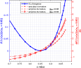
((a)) $\alpha_{o}=0.85$

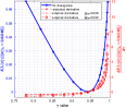
((b)) $\gamma_{o}=0.94146$

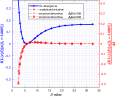
((c)) $\beta_{o}=5.\dot{6}$

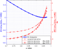
((d)) $\alpha_{o}=0.95$

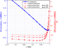
((e)) $\gamma_{o}=0.98831$

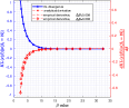
((f)) $\beta_{o}=19$

Figure 6: Intra-model relative variation in PageRank distribution by (14), on the Twitter graph. The rest is in the same setting as in Figure 5.

V-D Batch calculation: efficiency and accuracy

We show first that the Krylov space dimension is numerically low for each of the 6 real world link graphs. Figure 7 gives the diagonal elements of each upper-triangular matrix $R$ obtained by a rank-revealing QR factorization. The elements below $10^{-17}$ are not shown. The numerical dimension ranges from $19$ with DBpedia link graph to $62$ with Google link graph. The low numerical dimension makes our algorithm in Section IV highly efficient. In addition, we exploited the sparsity of matrix $P$ in the Krylov vector calculation, see details in [30].

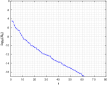
((a)) Google

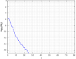
((b)) Twitter(www)

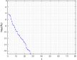
((c)) Wikipedia

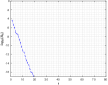
((d)) DBpedia

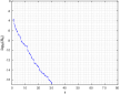
((e)) Twitter(mpi)

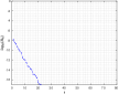
((f)) Friendster

Figure 7: The diagonal elements of each upper-triangular matrix $R$ obtained by a rank-revealing QR factorization for the 6 datasets in Table 1. Google link graph has the highest numerical dimension 62 among the 6 datasets, and the DBpedia link graph has the lowest numerical dimension 19.

The accuracy of our batch algorithm is evaluated in two ways. One is by $err=\|(x_{\text{Krylov}}-x_{\text{G-S}})./x_{\text{G-S}}\|_{\infty}$, the maximum element-wise relative difference in the PageRank vectors of Brin-Page model between the Gauss-Seidel method and our Krylov subspace method. In our experiments, the relative errors for all 6 datasets are below $10^{-10}$. In the other way, we show in Figure 5 and Figure 6 that the empirical rate of change agrees well with analytical prediction (15).

VI Concluding remarks

Our model extension, connection, unified analysis and numerical algorithm for quantitative estimation in batch are original, to our knowledge. Our study leads to new observation and several findings. (a) In network propagation pattern in response to variation in the damping mechanism, the inter-model difference among the 3 models is much more significant than the inter-dataset difference among the 6 datasets. This suggests the utility of model variety for differentiating network activities or propagation patterns. (b) The model solutions reside in the same customized, spectrally invariant subspace. On each of the $6$ real-world graphs, the space dimension is low, which is a small-world phenomenon. (c) The shared computation is not limited to one personalized distribution. The Krylov space associated with a particular vector $v$ contains certainly many other distribution vectors. In fact, every Krylov vector is a distribution vector. This finding may lead to a much more efficient way to represent and compute PageRank distributions across multiple personalized vectors. (d) The low spectral dimension, estimated once for a particular graph $P$ and a personalized/customized vector $v$, may serve as a reasonable upper bound on the number of iterations by any competitive algorithm, with one matrix-vector product per iteration, for Brin-Page model, at any $\alpha$ value in $(0,1)$, or any other model in the family (8). The power method and the Gauss-Seidel iteration take more iterations to reach the same error level on the larger real-world graphs among the studied, and take many more iterations when $\alpha$ gets closer to $1$. In brief conclusion, estimating PageRank distribution under various damping conditions is valuable and easily affordable.

References

- [1] L. Page, S. Brin, R. Motwani, and T. Winograd, “The PageRank citation ranking: Bringing order to the web.” Stanford InfoLab, Tech. Rep., 1999.
- [2] S. Brin and L. Page, “The anatomy of a large-scale hypertextual web search engine,” Computer networks and ISDN systems, vol. 30, no. 1-7, pp. 107–117, 1998.
- [3] D. Sheldon, “Manipulation of PageRank and Collective Hidden Markov Models,” Ph.D. dissertation, Cornell University, Ithaca, NY, USA, 2010.
- [4] T. H. Haveliwala, “Topic-sensitive PageRank: A context-sensitive ranking algorithm for web search,” IEEE Transactions on Knowledge and Data Engineering, vol. 15, no. 4, pp. 784–796, 2003.
- [5] J. L. Morrison, R. Breitling, D. J. Higham, and D. R. Gilbert, “Generank: using search engine technology for the analysis of microarray experiments,” BMC bioinformatics, vol. 6, no. 1, p. 233, 2005.
- [6] G. Wu, Y. Zhang, and Y. Wei, “Krylov subspace algorithms for computing generank for the analysis of microarray data mining,” Journal of Computational Biology, vol. 17, no. 4, pp. 631–646, 2010.
- [7] A. N. Langville and C. D. Meyer, “Deeper inside PageRank,” Internet Mathematics, vol. 1, no. 3, pp. 335–380, 2004.
- [8] P. Berkhin, “A survey on PageRank computing,” Internet Mathematics, vol. 2, no. 1, pp. 73–120, 2005.
- [9] T. Haveliwala, S. Kamvar, and G. Jeh, “An analytical comparison of approaches to personalizing PageRank,” Stanford InfoLab, Technical Report 2003-35, June 2003.
- [10] S. Kamvar, T. Haveliwala, C. Manning, and G. Golub, “Exploiting the block structure of the web for computing PageRank,” Stanford InfoLab, Technical Report 2003-17, 2003.
- [11] P. Boldi, M. Santini, and S. Vigna, “PageRank as a function of the damping factor,” in Proceedings of the 14th International Conference on World Wide Web. ACM, 2005, pp. 557–566.
- [12] M. Bressan and E. Peserico, “Choose the damping, choose the ranking?” Journal of Discrete Algorithms, vol. 8, no. 2, pp. 199–213, 2010.
- [13] F. Chung, “The heat kernel as the PageRank of a graph,” Proceedings of the National Academy of Sciences, vol. 104, no. 50, pp. 19 735–19 740, 2007.
- [14] ——, “A local graph partitioning algorithm using heat kernel PageRank,” Internet Mathematics, vol. 6, no. 3, pp. 315–330, 2009.
- [15] A. Arasu, J. Novak, A. Tomkins, and J. Tomlin, “PageRank computation and the structure of the web: Experiments and algorithms,” in Proceedings of the 11th International Conference on World Wide Web, 2002, pp. 107–117.
- [16] S. Kullback and R. A. Leibler, “On information and sufficiency,” The Annals of Mathematical Statistics, vol. 22, no. 1, pp. 79–86, 1951.
- [17] C. P.-C. Lee, G. H. Golub, and S. A. Zenios, “A fast two-stage algorithm for computing PageRank and its extensions,” Scientific Computation and Computational Mathematics, vol. 1, no. 1, pp. 1–9, 2003.
- [18] A. N. Langville and C. D. Meyer, “A reordering for the PageRank problem,” SIAM Journal on Scientific Computing, vol. 27, no. 6, pp. 2112–2120, 2006.
- [19] A. L. Dulmage and N. S. Mendelsohn, “Coverings of bipartite graphs,” Canadian Journal of Mathematics, vol. 10, no. 4, pp. 516–534, 1958.
- [20] Google, “Google programming contest,” http://www.google.com/programming-contest/, 2002.
- [21] S. D. Kamvar, T. H. Haveliwala, C. D. Manning, and G. H. Golub, “Extrapolation methods for accelerating PageRank computations,” in Proceedings of the 12th International Conference on World Wide Web. ACM, 2003, pp. 261–270.
- [22] S. Kamvar, T. Haveliwala, and G. Golub, “Adaptive methods for the computation of PageRank,” Linear Algebra and its Applications, vol. 386, pp. 51–65, 2004.
- [23] P. A. Lofgren, S. Banerjee, A. Goel, and C. Seshadhri, “FAST-PPR: scaling personalized pagerank estimation for large graphs,” in Proceedings of the 20th ACM SIGKDD International Conference on Knowledge Discovery and Data Mining. ACM, 2014, pp. 1436–1445.
- [24] J. Kunegis, “KONECT–the koblenz network collection,” in Proceedings of the 22nd International Conference on World Wide Web. ACM, 2013, pp. 1343–1350.
- [25] S. Auer, C. Bizer, G. Kobilarov, J. Lehmann, R. Cyganiak, and Z. Ives, “DBpedia: A nucleus for a web of open data,” in The Semantic Web. Springer, 2007, pp. 722–735.
- [26] H. Kwak, C. Lee, H. Park, and S. Moon, “What is Twitter, a social network or a news media?” in Proceedings of the 19th International Conference on World Wide Web. New York, NY, USA: ACM, 2010, pp. 591–600.
- [27] M. Cha, H. Haddadi, F. Benevenuto, and K. P. Gummadi, “Measuring User Influence in Twitter: The Million Follower Fallacy,” in Proceedings of the 4th International AAAI Conference on Weblogs and Social Media (ICWSM), Washington DC, USA, May 2010.
- [28] J. Yang and J. Leskovec, “Defining and evaluating network communities based on ground-truth,” Knowledge and Information Systems, vol. 42, no. 1, pp. 181–213, 2015.
- [29] Y. Qian, “Variable damping effect on network propagation,” Master’s thesis, Duke University, Durham, NC, USA, May 2018.
- [30] X. Chen, “Exploiting common structures across multiple network propagation schemes,” Master’s thesis, Duke University, Durham, NC, USA, May 2018.
- [31] T. Haveliwala and S. Kamvar, “The second eigenvalue of the google matrix,” Stanford InfoLab, Technical Report 2003-20, 2003.
- [32] M. Richardson and P. Domingos, “The intelligent surfer: Probabilistic combination of link and content information in PageRank,” in Advances in Neural Information Processing Systems, 2002, pp. 1441–1448.
- [33] T. Haveliwala, “Efficient computation of PageRank,” Stanford, Tech. Rep., 1999.
- [34] A. N. Langville and C. D. Meyer, Google’s PageRank and beyond: The science of search engine rankings. Princeton University Press, 2011.
- [35] G. Jeh and J. Widom, “Scaling personalized web search,” in Proceedings of the 12th International Conference on World Wide Web. ACM, 2003, pp. 271–279.
- [36] F. Chung and W. Zhao, “PageRank and random walks on graphs,” in Fete of Combinatorics and Computer Science. Springer, 2010, pp. 43–62.