Cutting the Double Loop:
Theory and Algorithms for Reliability-Based Design Optimization with Statistical Uncertainty

Abstract

Statistical uncertainties complicate engineering design – confounding regulated design approaches, and degrading the performance of reliability efforts. The simplest means to tackle this uncertainty is double loop simulation; a nested Monte Carlo method that, for practical problems, is intractable. In this work, we introduce a flexible, general approximation technique that obviates the double loop. This approximation is constructed in the context of a novel theory of reliability design under statistical uncertainty: We introduce metrics for measuring the efficacy of RBDO strategies (effective margin and effective reliability), minimal conditions for controlling uncertain reliability (precision margin), and stricter conditions that guarantee the desired reliability at a designed confidence level. We provide a number of examples with open-source code to demonstrate our approaches in a reproducible fashion.

1 Introduction

Uncertainty complicates design. Unknown loads motivate safety factors; manufacturing fluctuations motivate material property knockdowns. When uncertainty is modeled by a random variable, additional uncertainty arises when fitted distribution parameters are estimated from data, leading to statistical uncertainty.

Statistical uncertainty represents a lack of knowledge in a system or design, with the potential for improvement in performance or safety. Such uncertainty can lead to degraded performance; for example, Park et al.[1] demonstrated significant weight penalties due to sampling uncertainties in coupon and element testing. Gains in engineering design can be made through the acquisition of more information, though the question remains of how to confidently and efficiently guarantee the reliability of a system’s performance and safety under statistical uncertainty.

Optimizing system performance while constrained by failure probability goes by the name reliability based design optimization (RBDO). When statistical uncertainties are modeled as parameters to input distributions, they induce second-order uncertainties similar to a hierarchical model.[2] These uncertainties are most simply handled through a double loop Monte Carlo simulation[3] over a sampling distribution or hyperprior. Of course, this approach is multiplicative in its expense, rendering all but the simplest problems intractable.

Further, in reviewing the literature it was unclear to us how to measure the effects of statistical uncertainties in RBDO, let alone how to control realized design reliability.[3, 4, 5] The aforementioned works introduce approaches that are distinct in how they introduce engineering conservatism, but are similar in that they recover the the ‘true’ reliability in the case of perfect information. This is in contrast with other design practices outside the framework of RBDO, such as those utilizing basis values. Further, in statistical inference, there exists the notion of confidence intervals, which guarantee frequentist properties of coverage;[6] we have not found a similar notion in the context of RBDO. Our work was in part motivated by a desire for useful theory by which to compare and contrast different approaches to managing statistical uncertainties.

In this work, we introduce the metrics of effective margin and effective reliability to assess the performance of RBDO strategies incorporating statistical uncertainties. To control effective reliability, we introduce minimum conditions that define precision margin (PM). To show the concept’s generality, we formally prove that the conservative reliability index (CRI) of Ito et al.[3] is a PM. We also present two implementations of PM, both carrying unique advantages and challenges. The second of these implementations – margin in probability (MIP) – adds just enough margin to guarantee the desired reliability at a known confidence level. We call this property confidently conservative (C2), and regard it as a translation of statistical coverage to engineering design practice.

While our examples in this work consider materials characterization, the PM concept is flexible enough to apply to any case of sampling uncertainty. The particular approximations of PM presented in this work are restricted to cases of modeled randomness, where a specific (analytic) joint PDF is selected to model variable quantities – this choice is in line with existing Department of Defense probabilistic design methodologies.[7]

Of course, we are not the first to tackle the double loop issue. Der Kiureghian[4] carried out reliability design over a Bayesian posterior distribution, effectively incorporating statistical uncertainties into a single loop; however, his predictive reliability index does not add any form of margin. Noh et al.[5] tackle the same issue by perturbing the estimated moments of an normal distribution, assuming that there exists a transform to standard normal space. Our approach is more general, in the sense that we work directly in the original probability space of the posed random variable model. The work of Ito et al.[3] is closely related to what we suggest, though similarly assumes a transform to standard normal space, and does not guarantee the C2 property. We draw a close comparison between their CRI and our proposed MIP approach. Note that some other authors refer to the form of uncertainty we consider as epistemic, e.g. Ito et al.[3]. We use a more specific terminology – statistical uncertainty – as we do not claim our approach is appropriate for all epistemic uncertainties (such as unknown unknowns), but instead note that our work addresses many of the same issues commonly referred to as epistemic uncertainties.

Our approximation technique is a form of Monte Carlo reweighting,[8] but using the likelihood ratio (LR) gradient estimation technique to approximate parameter gradients at negligible additional cost.[9, 10] Note that “double loop” is sometimes used to refer to a reliability analysis nested within an optimization loop;[11] we use this term in its other commonly accepted meaning to refer to nested Monte Carlo.

An outline of this article is as follows: Section 2 presents the motivating issue through a simple structural sizing problem, illustrating the effects of sampling uncertainty on both standard industry practice and a ‘plug-in’ RBDO approach. Here we introduce the metrics of effective margin and effective reliability. Section 3 introduces the precision margin concept, presents two implementations, and provides comparisons against the previously-introduced methods. The two implementations apply margin in either physical or probability space, and present different advantages and challenges. Section 4 provides practical estimation procedures to enable the computation of PM – the techniques introduced here add negligible computational cost, and are simple to incorporate within an RBDO framework. Section 5 demonstrates the PM methodology on a common RBDO test case, while Section 6 retrospects, providing context and sketching future directions.

Our aim is to constructively comment on the practice of engineering design, and to illustrate a potential avenue for the continued development of our profession. In the spirit of facilitating this development, a companion GitHub repository contains all the code necessary to generate the results in the present work, and to serve as a reference implementation for the suggested algorithms.

2 Motivating Issue

We first introduce the design problem of sizing for uniaxial tension, and formulate the problem in a reliability-based design framework, in order to illustrate the effects of statistical uncertainty on reliability. We introduce two families of approaches of dealing with uncertain material properties, first studying approaches using a basis value, and second directly modeling the variable material with ‘plug-in’ parameter estimates. We employ all approaches at different cases of desired reliability, and demonstrate that none produce desirable results, motivating the introduction of precision margin in the section to follow.

2.1 Uniaxial Tension Sizing

For illustrative purposes we introduce a structural sizing problem, whose simplicity highlights the issue of statistical material property uncertainties. We consider sizing the wall thickness $t$ of a hollow cylinder of given radius $r$; this has cross sectional area given by $A(t)=\pi\left((r+t)^{2}-r^{2}\right)$. We take the applied tensile force to have a known distribution $F\sim\mathcal{N}(\mu_{f},\tau^{2}_{f})$, while the material ultimate tensile strength has a ground truth distribution $U\sim\mathcal{N}(\mu_{u},\tau^{2}_{u})$. For simplicity, we model these variables as independent Gaussians; one could easily use lognormal variables to enforce positivity, which would not materially change our conclusions. Table 1 summarizes the ground truth parameter values used in this study.

Table 1: Ground truth parameters for uniaxial tension example. We assume a material coefficient of variation of $10\%$, a high but realistic value for advanced composite materials.[12]

Parameter	Value	Units
$\mu_{u}$	$600$	MPa
$\mu_{f}$	$100$	N
$\tau_{u}$	$60$	MPa
$\tau_{f}$	$10$	N

In general, failure of a structure is modeled by the limit state function $g(\boldsymbol{d},\boldsymbol{X})$, where $\boldsymbol{d}\in\mathbb{R}^{d_{d}}$ are the design variables, and $\boldsymbol{X}\in\mathbb{R}^{d_{r}}$ are random variables.[13] For uniaxial tension, we have the limit state function

$$g(t,\boldsymbol{X})=U-F/A(t),$$ (1)

where $g\leq 0$ corresponds to failure, and $\boldsymbol{X}=(U,F)^{\top}$ are the random variables, chosen to model different sources of uncertainty. The critical ultimate stress $U$ replaces a fixed, deterministic stress $\sigma_{ult}$ to model the variability inherent in manufacturing processes. The applied load $F$ replaces a fixed load $f$ to model the uncertain conditions the design will encounter. Reliable sizing is accomplished by solving the optimization problem

min $$C(t),$$ (2)

s.t. $$\mathbb{P}_{\boldsymbol{X}}[g(t,\boldsymbol{X})>0]\geq\mathcal{R},$$

where $C$ is the cost of the design, taken to be $C(t)=t$ for this example, and $\mathcal{R}\in[0,1]$ is the desired reliability. Here and below, we denote by subscript the random variables considered in evaluating an expectation, e.g. a probability statement. Equation 2 has an exact solution, defined by

$$A^{*} =\frac{\mu_{u}\mu_{f}+\sqrt{\Phi^{-1}(\mathcal{R})^{2}\mu_{u}^{2}\tau_{f}^{2}+\Phi^{-1}(\mathcal{R})^{2}\mu_{f}^{2}\tau_{u}^{2}-\Phi^{-1}(\mathcal{R})^{4}\tau_{u}^{2}\tau_{f}^{2}}}{\mu_{u}^{2}-\Phi^{-1}(\mathcal{R})^{2}\tau_{u}^{2}},$$ (3)

$$t^{*} =\sqrt{A^{*}/\pi+r^{2}}-r,$$

where $\Phi^{-1}(\cdot)$ is the standard inverse normal CDF. In the case where $r=1m$ and $\mathcal{R}=0.95$, we find the solution $t^{*}\approx 3.3cm$.

2.2 Uncertain Parameters

In practice, the parameters $\boldsymbol{\theta}$ for the distribution of the random variables may not be known. In the uniaxial tension example, we assume we know the parameters for $F$ exactly, and have access to some number $m$ of samples $\boldsymbol{U}_{i}\sim\mathcal{N}(\mu_{u},\tau^{2}_{u})$, which lead to the sample estimates and their (sampling) distributions

$$\overline{U} =\frac{1}{m}\sum_{i=1}^{m}\boldsymbol{U}_{i}\sim\mathcal{N}(\mu_{u},\tau^{2}_{u}/m),$$ (4)

$$S^{2}_{u} =\frac{1}{m-1}\sum_{i=1}^{m}(\boldsymbol{U}_{i}-\overline{U})^{2}\sim\chi^{2}_{m-1}\tau^{2}_{u}/(m-1).$$

Note that we assume no additional measurement noise on the material measurements $\boldsymbol{U}_{i}$. Variation here is assumed to arise from manufacturing variability alone. The parameter estimates $\hat{\boldsymbol{\theta}}=(\overline{U},S^{2}_{u})^{\top}$ are random and have the moments

$$\mathbb{E}[\boldsymbol{\theta}] =(\mu_{u},\tau^{2}_{u})^{\top},$$ (5)

$$\mathrm{Cov}[\boldsymbol{\theta}] =\text{Diag}[\tau^{2}_{u}/m,\tau^{4}_{u}/(m-1)]\equiv\boldsymbol{T}.$$

We will denote by $\hat{\boldsymbol{T}}$ the sample estimate of $\mathrm{Cov}[\boldsymbol{\theta}]$, and will occasionally use a subscripted version $\hat{\boldsymbol{T}}_{m}$ to emphasize the sample size. The lack of perfect knowledge implies that exactly solving the RBDO problem (2) is not possible. Instead, one must turn to some form of statistical approximation – two possible approaches are detailed below.

2.3 Regulated and Mixed Design

Under Title 14 CFR 25.613, commercial aircraft designers are required to establish material properties using a basis value, a random variable constructed from a random material population. Formally, a basis value is a tolerance interval, a random interval constructed with respect to another random variable, such that the interval contains a fraction $\mathcal{P}$ of the population at a desired confidence level $\mathcal{C}$.[14] A basis value is a one-sided interval, thus it is reported as a single number.

Practically, one may draw a number $m$ of samples of the desired material property $U_{i}\sim\rho$ for $i=1,\dots,m$ and compute the sample mean $\overline{U}$ and variance $S^{2}$. Effectively, the basis value is the mean estimate, knocked down by the sample standard deviation, scaled by an appropriate factor $k_{\mathcal{P},\mathcal{C}}(m)$. Formally, we have

$$B=\overline{U}-k_{\mathcal{P},\mathcal{C}}(m)S,$$ (6)

where $k_{\mathcal{P},\mathcal{C}}(m)$ is determined by the desired Population fraction $\mathcal{P}$, Confidence level $\mathcal{C}$, and chosen sample count $m$. Under a normal $X$ assumption, the factor $k_{\mathcal{P},\mathcal{C}}(N)$ can be determined from a non-central t-distribution – this assumption is exact in the uniaxial tension problem defined above. One may also employ empirical methods for computing basis values in the case of large sample sizes.[14]

Note that $B$ is a random variable, for which we compute a realization based on sample estimates. The basis value is applied by introducing a modified limit state function

$$g(t,B,F)=B-F/A(t).$$ (7)

Note that (7) is not the true limit state, but is instead an approximation induced by the basis value. We shall see (Fig. 1) that this approximation will not necessarily lead to a conservative design.

An additional level of conservatism is required by Title 14 CFR 25.303, which imposes a factor of safety (FOS) of $1.5$ on external load limits. In this regulated approach to design, one sizes the cross-section via

$$A^{*}_{\text{regulated}}=B/(1.5\mu_{f}),$$ (8)

here using $\mu_{f}$ as the nominal loading conditions. We also pursue a ‘mixed’ approach using a basis value, which is (to our knowledge) not used in industry, but better isolates the effect of the basis value approximation, purely for illustrative purposes. Since the basis value is the only number reported, we do not have enough information to evaluate the probability related to the material population variability in (2). We instead solve a modified optimization problem, given by

min $$C(t),$$ (9)

s.t. $$R(B)\equiv\mathbb{P}_{F}[g(t,B,F)>0]\geq\mathcal{R}.$$

Note that the evaluated reliability $R(B)$ is now a random variable, induced by the random basis value. Thus the $t$ which solves (9) is a random variable. Furthermore, the uncertainty arising from the material property is not accounted in the probability statement, as implied by the subscript.

It is important to note that it is patently unreasonable to expect these approaches to compare favorably with true RBDO approaches – the regulated and mixed approaches are simply not tailored for controlling failure probabilities. However, we include these results to show how the regulated approach fares in terms of realized system reliability. To our knowledge, such a comparison has not been made in the literature – the studies here give a sense of what potential improvements could be made, should RBDO be more widely adopted in real aircraft design. Intuitively, this potential for improvement exists because, in both the regulated (8) and mixed (9) approaches, the material uncertainty is effectively decoupled from system reliability by the basis value.

2.4 Plug-In Estimate

As an alternative to the approaches above, one may model random material properties,[7] estimate the distribution parameters $\boldsymbol{\theta}$, and evaluate all probabilities using the ‘plug-in’ estimate $\hat{\boldsymbol{\theta}}$. This approach leads to the modified optimization problem

min $$C(t),$$ (10)

s.t. $$R(\hat{\boldsymbol{\theta}})\equiv\mathbb{P}_{\boldsymbol{X}(\hat{\boldsymbol{\theta}})}[g(t,\boldsymbol{X}(\hat{\boldsymbol{\theta}}))>0]\geq\mathcal{R},$$

where we introduce the notation $\boldsymbol{X}(\hat{\boldsymbol{\theta}})\sim\rho(\hat{\boldsymbol{\theta}})$ to denote a random variable drawn conditional on the assumed parameter values $\hat{\boldsymbol{\theta}}$, and note that the notation $\boldsymbol{X}$ implies the random variable is drawn according to the ground truth parameters $\boldsymbol{\theta}$. Note that (10) also involves a random estimated reliability $R(\hat{\boldsymbol{\theta}})$, with the randomness induced by the estimated parameter values. Thus the $t$ which solves (10) is also a random variable. This design is computed using (3), substituting the estimated parameter values.

2.5 Metrics and Results

Here we compare the approaches above in terms of their performance, relative to the exact solution of (2). For comparison, we introduce two performance metrics; the effective margin $M_{\text{eff},\mathcal{C}}(\boldsymbol{d})$ and effective reliability $R_{\text{eff},g}(\boldsymbol{d})$, defined in (11) below.

$$M_{\text{eff},C}(\boldsymbol{d}) \equiv\frac{C(\boldsymbol{d})-C^{*}}{C^{*}},$$ (11)

$$R_{\text{eff},g}(\boldsymbol{d}) \equiv\mathbb{P}_{\boldsymbol{X}}[g(\boldsymbol{d},\boldsymbol{X})>0].$$

Note that since $M_{\text{eff},C}(\boldsymbol{d})$ is defined with respect to a minimal objective value $C^{*}$, it is only defined for RBDO problems where such a value exists. The effective margin $M_{\text{eff},C}(\boldsymbol{d})$ measures system performance in terms of the chosen cost metric $C(\boldsymbol{d})$. If $M_{\text{eff},C}(\boldsymbol{d})$ is positive, it implies there must be slackness in the reliability constraints (under the true parameter values $\boldsymbol{\theta}$), and the cost of the design could be reduced. Conversely, negative effective margin implies the cost observed could not have been achieved without violating a constraint – in this case effective margin is an indication of how under-built a design is.

The effective reliability $R_{\text{eff},g}(\boldsymbol{d})$ directly measures the achieved reliability of a design, in terms of a single constraint. An $R_{\text{eff},g}(\boldsymbol{d})$ less than (greater than) the desired reliability implies under- (over-) design in the system. In contrast with effective margin, which gives a single measure for a design problem, one would have a set of effective reliabilities for a design problem – one for each reliability constraint. We will illustrate a case with multiple constraints below.

Note that we will use these quantities to measure the performance of design strategies by considering an ensemble of random designs arising from different approaches. Furthermore, these quantities are frequentist constructions, as they are predicated on the existence of a true parameter value $\boldsymbol{\theta}$.

Since the $t$ arising from the strategies above are random, the resulting performance metrics are also random. We simulate the sizing problem by drawing a variable number of material samples $m$, solving the optimization problems analytically, and replicate this entire procedure to build confidence intervals that measure design strategy performance. The results shown in Figure 1 demonstrate deficient behavior with all approaches discussed above.

Both the regulated and mixed approaches result in either over- or under-designed solutions, depending on the desired reliability. Intuitively, this deficiency is due to ‘decoupling’ of attendant uncertainties from the system reliability. In computing a basis value, one gathers enough data to estimate the mean and variance of a material population, but then collapses all data to a single number for structural sizing. Any following design for reliability cannot account for distributional information in this framework, which results in a lack of control over the ultimate failure chance. Stated differently, the basis value approach attempts to add a form of margin (in the $-k_{\mathcal{P},\mathcal{C}}(m)S$ term) to the material property, and additional forms of margin are added in the downstream design process; since these margins are not designed in terms of the system reliability, it is unsurprising they fail to control the system failure chance.

Note that given two standards of basis value – A- and B-basis – and the modeling assumptions used to generate them (random variable model and sample size), one can easly recover the estimated moments of the data, and use these for reliability design. However, one cannot reasonably claim to be performing design using basis values in this case, as the results will be identical to the plug-in approach.

The plug-in approach asymptotically recovers zero effective margin, but returns an unacceptable fraction of negative effective margin designs. This is because the plug-in approach adds no form of margin. The estimated parameter values are assumed to be true for the purposes of sizing; when the material capacity mean is overestimated (or the variance underestimated), the resulting design will be less reliable than desired. In practice, a designer would want a principled way to add margin to quantities directly related to failure criteria. These results motivate the introduction of precision margin.

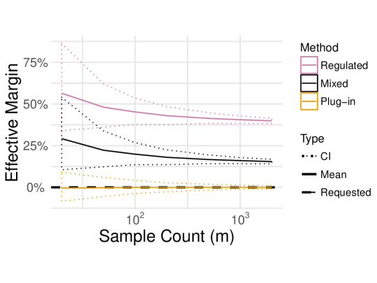
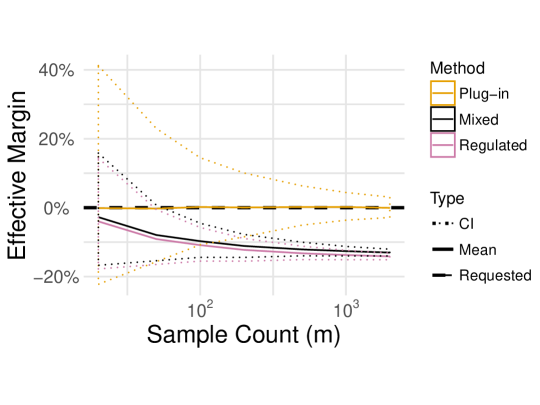
Figure 1: Effective margin against sample size for designed reliability $\mathcal{R}=0.99$ (Top) and $\mathcal{R}=1-10^{-7}$ (Bottom) in the uniaxial tension example. Since the reliable design problems are solved analytically, all pathologies arise from the materials characterization process. We use an A-basis value in both reliability problems. All approaches necessarily return random designs due to material uncertainties: Mean profiles and two-sided $95\%$ confidence intervals are approximated using $10^{3}$ replications. The results shown here illustrate that the regulated and mixed approaches do not control the failure probability. At low reliability (Top), the use of a basis value leads to unintentional effective margin, while at high reliability (Bottom) its use prevents the desired reliability from being achieved. Since no margin is added to the design, any effective margin (whether positive or negative) is unintentional, and opaque to the designer. The plug-in approach has zero effective margin in the asymptotic limit, but returns an unacceptable fraction of under-performing designs at reasonable sample sizes. Ideally, one would desire a design procedure which has positive effective margin at some designed confidence level. In Sec. 3 we introduce a procedure which approaches the ideal.

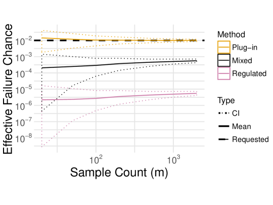
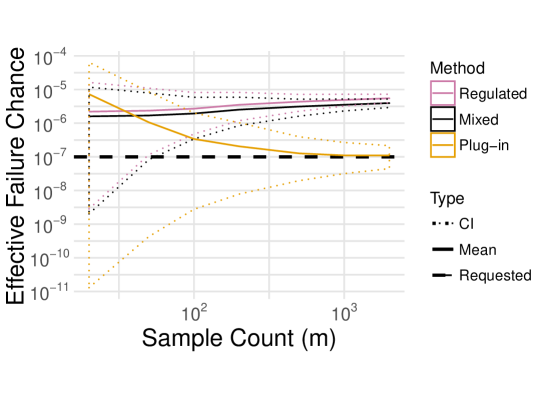
Figure 2: Effective reliability against sample size for designed reliability $\mathcal{R}=0.99$ (Top) and $\mathcal{R}=1-10^{-7}$ (Bottom) in the uniaxial tension example. For ease of plotting, we report the effective failure chance $F_{\text{eff}}=1-R_{\text{eff}}$, which carries the same information. The conclusions of Figure 1 are echoed here. At low reliability targets the use of a basis value results in an overly-conservative design; that is, the failure chance is lower than requested, implying that material could be removed and the design would still achieve the desired reliability. Despite the fact that the A-basis value population fraction matches the desired reliability target, both approaches using a basis value lead to significant over-design. At high reliability targets, the opposite issue arises; the failure chance is higher by orders-of-magnitude.

3 Precision Margin

In this section, we present a design methodology which overcomes the issues inherent in both the basis value and plug-in approaches. Here we introduce the general concept of precision margin, provide examples of its implementation, and present results for the uniaxial tension sizing problem.

3.1 Precision Margin Concept

Margin is a simple but ubiquitous concept from engineering. Margin is a displaced threshold for some constraint, added to encourage a conservative design. Within the RBDO framework, one can add margin in at least two ways:

$$\mathbb{P}_{\boldsymbol{X}}[g(\boldsymbol{d},\boldsymbol{X})>g_{m}] \geq\mathcal{R},$$ (12)

$$\mathbb{P}_{\boldsymbol{X}}[g(\boldsymbol{d},\boldsymbol{X})>0] \geq\mathcal{R}+p,$$

which we refer to (respectively) as margin in limit (MIL) state, and margin in probability (MIP): We will see below that the MIP formulation provides additional, desirable properties. In (12), adding positive margin ($g_{m},p>0$) will result in an overly-conservative design, with regard to the desired reliability. However, adding margin is useful in the realistic case where the parameters $\boldsymbol{\theta}$ are not exactly known.

We introduce the concept of precision margin as a form of margin added to handle the statistical uncertainties in $\hat{\boldsymbol{\theta}}$ arising from an estimation procedure. Thus, we introduce the following definition:

Definition: Precision margin (PM) is any form of margin which:

1. Improves the reliability of a system limit state, based on discrepancy with the realized reliability

2. Decays to zero with increased precision

These requirements are inspired both by the deficiencies found among the methods in Section 2 and by existing approaches in literature.[3] The plug-in approach uses estimates for ‘best guess’ parameter values, but does not account for how those estimates may affect the realized reliability. Conversely, both basis value approaches add some form of margin, but with a value decoupled from the system reliability. Point 1 addresses these deficiencies. Note that the regulated and mixed approaches also failed to converge to the true system reliability, even as the number of samples $m$ approached infinity. Point 2 addresses this, by imposing a convergence criteria.

Note that precision margin is intended to deal with statistical uncertainties only; this excludes unidentified uncertainties. This flexible definition can be implemented in multiple ways, as illustrated below.

3.2 Margin in Limit

Here we define the margin in limit (MIL) as a margin term $g_{MIL,\mathcal{C}}$ based on the mean difference between the estimated limit state $\hat{g}$ and the true limit state $g$. This margin is defined at a desired confidence level $\mathcal{C}$ by

$$\mathbb{P}_{\hat{\boldsymbol{\theta}}}\left[g_{MIL,\mathcal{C}}>E_{\boldsymbol{X}(\hat{\boldsymbol{\theta}})}[g(\boldsymbol{d},\boldsymbol{X}(\hat{\boldsymbol{\theta}}))]-\mathbb{E}_{\boldsymbol{X}}[g(\boldsymbol{d},\boldsymbol{X}(\boldsymbol{\theta}))]\right]=\mathcal{C}.$$ (13)

Note that $E_{\boldsymbol{X}(\hat{\boldsymbol{\theta}})}[g(\boldsymbol{d},\boldsymbol{X}(\hat{\boldsymbol{\theta}}))]$ is a random variable, due to the randomness induced by $\hat{\boldsymbol{\theta}}$. In order for $g_{MIL,\mathcal{C}}$ to be a PM, it must converge to zero as $\hat{\boldsymbol{\theta}}\to\boldsymbol{\theta}$. We present a proof of this fact in Appendix 7.1. For the uniaxial tension example, the margin in limit PM has an analytic expression, given by $g_{MIL,\mathcal{C}}=\Phi^{-1}(\mathcal{C})\tau_{u}/\sqrt{m}$, independent of the thickness $t$. In a more general setting $g_{MIL,\mathcal{C}}$ may be a function of the design variables $\boldsymbol{d}$, a fact which has implications for RBDO, and which will be revisited in in Section 4.

Example results shown in Figure 3 demonstrate that the mean difference PM is indeed more conservative than the plug-in approach, but does not guarantee non-zero effective margin at the desired confidence level, a property we will achieve with a different implementation below. Crucially, the margin in limit PM results approach the desired reliability, in contrast with the approaches employing basis values. Note also that the margin in limit PM formally relies on exact knowledge of $\boldsymbol{\theta}$; we will introduce an approximation to this margin term below.

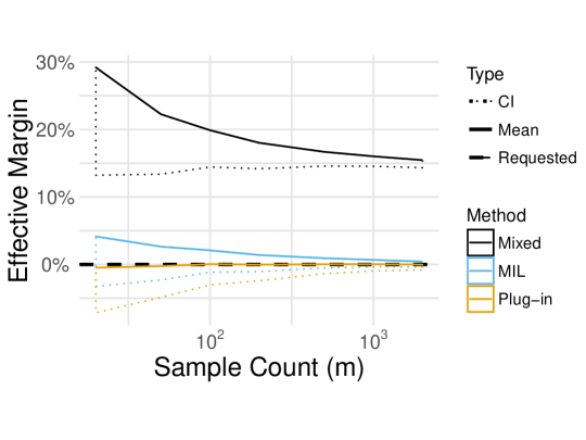
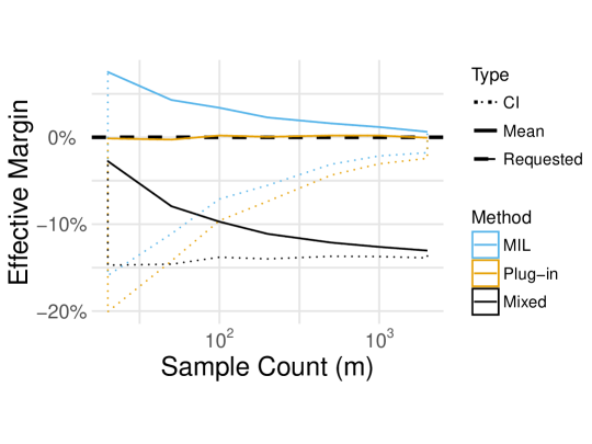
Figure 3: Comparison of margin in limit PM (MIL PM) against an A-Basis Value (BV) and Plug-In (PI) approaches at $\mathcal{R}=0.99$ (Top) and $\mathcal{R}=1-10^{-7}$ (Bottom). Probabilities are evaluated analytically at estimated parameter values, and $10^{3}$ replications are carried out to construct mean curves and one-sided $95\%$ confidence intervals. As predicted, the MIL approach is more conservative than the plug-in approach. Crucially, the margin in limit approach approaches the desired reliability as the sample count is increased, in contrast with the regulated and mixed approaches. Note that the MIL approach demonstrated here relies on exact knowledge of $\boldsymbol{\theta}$; we present an approximation of this approach in Sec. 4. Despite the use of exact knowledge, even the MIL approach leads to an unacceptable fraction of under-performing designs, particularly in the strict-reliability case; in Sec. 4 we introduce an alternative strategy which addresses this issue.

3.3 Margin in Probability

An equally valid means to add margin is to apply margin in the estimated reliability, as in the second line of (12). This is an attractive option, as it more directly controls the quantity of interest for design for reliability – the failure chance – rather than exerting an indirect influence through the limit state. Margin in probability $p$ is applied by designing for the modified constraint

$$R(\hat{\boldsymbol{\theta}})=\mathbb{P}_{\boldsymbol{X}(\hat{\boldsymbol{\theta}})}[g(\boldsymbol{d},\boldsymbol{X}(\hat{\boldsymbol{\theta}}))>0]\geq\mathcal{R}+p,$$ (14)

where $p$ is determined via the coupled auxiliary equation

$$\mathbb{P}_{\hat{\boldsymbol{\theta}}}[p>R(\hat{\boldsymbol{\theta}})-R(\boldsymbol{\theta})]=\mathcal{C}.$$ (15)

Applying margin in this fashion has a very desirable property; in this form, the confidence level $\mathcal{C}$ can be interpreted as a probability of satisfying the desired reliability $R(\boldsymbol{\theta},\boldsymbol{d}(\hat{\boldsymbol{\theta}}))\geq\mathcal{R}$ over the distribution of random designs. We can see this by first assuming a slack form of the reliability constraint (14) is satisfied,

$$R(\hat{\boldsymbol{d}},\hat{\boldsymbol{\theta}})=\mathcal{R}+p+\epsilon,$$ (16)

for any given random design $\hat{\boldsymbol{d}}\equiv\boldsymbol{d}(\hat{\boldsymbol{\theta}})$, and computing

$$\mathcal{C} =\mathbb{P}_{\hat{\boldsymbol{\theta}}}[p>R(\hat{\boldsymbol{\theta}},\hat{\boldsymbol{d}})-R(\boldsymbol{\theta},\hat{\boldsymbol{d}})],$$ (17)

$$=\mathbb{P}_{\hat{\boldsymbol{\theta}}}[R(\boldsymbol{\theta},\hat{\boldsymbol{d}})>\mathcal{R}+\epsilon].$$

Interpreting the probabilities of (17) requires that we consider random designs arising from the employed design strategy. Since the design $\hat{\boldsymbol{d}}$ is random (induced by the random parameters $\hat{\boldsymbol{\theta}}$), this allows us to interpret the probability over $\hat{\boldsymbol{\theta}}$.

We use the term confidently conservative (C2) to denote a design strategy with the property $\mathcal{C}=\mathbb{P}_{\hat{\boldsymbol{\theta}}}[R(\boldsymbol{\theta},\hat{\boldsymbol{d}})>\mathcal{R}]$. A strategy which is C2 is conservative in reliability at a known confidence level $\mathcal{C}$. In the case where the reliability constraint is not slack (i.e. $\epsilon=0$) over the distribution of $\hat{\boldsymbol{d}}$, the MIP strategy is C2. For the MIP strategy, and by the non-decreasing property of CDF’s, a slack reliability constraint implies a higher confidence level, while an infeasible constraint implies a lower confidence level.

Note that while C2 is a desirable property, we do not demand that a PM be C2; this is because the property will be practically unattainable in any real engineering context, due to challenges such as unknown unknowns. We introduce C2 as a theoretical ideal that practical design strategies can approach. The example below will illustrate the C2 property of this design strategy.

Here we draw a comparison with the conservative reliability index (CRI) of Ito et al.,[3] which is closely related to our proposed MIP approach. In nomenclature consistent with our presentation, they recommend solving

min. $$C(\boldsymbol{d}),$$ (18)

s.t. $$R^{\alpha}\geq\mathcal{R},$$

$$\mathbb{P}_{\hat{\theta}}[R(\hat{\boldsymbol{\theta}})>R^{\alpha}]=\alpha.$$

We note that the CRI approach is a form of precision margin, as it encourages conservatism based on the variability in the estimated reliability, and indeed recovers the true reliability with perfect information (Appendix 7.3). However, with this formulation, we arrive not at a C2 condition, but rather find that

$$\mathbb{P}_{\hat{\boldsymbol{\theta}}}[R(\hat{\boldsymbol{\theta}})>\mathcal{R}]=\alpha,$$ (19)

which is the reliability conditional on the estimated parameter values which, for $\boldsymbol{\theta}$ which take continuous values, will be correct with zero probability. One implication of the CRI approach is that bias in the estimated parameters can cause significant depatures in the realized reliability $R(\boldsymbol{\theta})$ from the desired threshold $\mathcal{R}$; we illustrate this fact with a simple example in Appendix 7.5.

Despite directly controlling the reliability, applying margin in probability has a weakness – this approach is more numerically unstable than applying margin directly to the limit state. If $p$ is estimated via some noisy procedure, then it is possible for $\mathcal{R}+p\geq 1$ to occur. In this case, the resulting reliability problem is ill posed. The example below will also illustrate this pathology.

In the tension sizing example, the estimated reliability has an analytical form

$$R(\hat{\boldsymbol{\theta}})=\Phi\left(\frac{\overline{X}-\mu_{f}/A(d)}{\sqrt{S^{2}+\tau_{f}^{2}/A(d)}}\right),$$ (20)

which we use in a semi-analytic study of the probability margin approach, solving the design problem via fixed-point iteration. Results of this numerical demonstration are reported in Figure 4, demonstrating the C2 property described above.

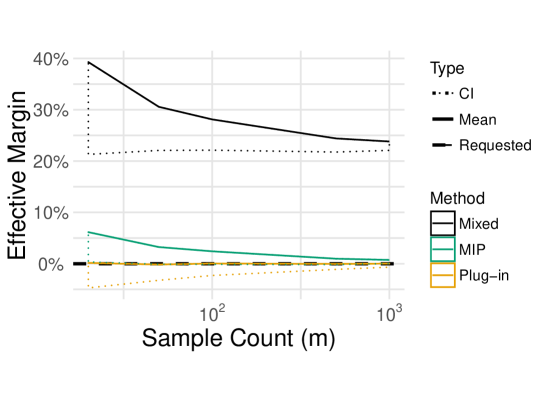
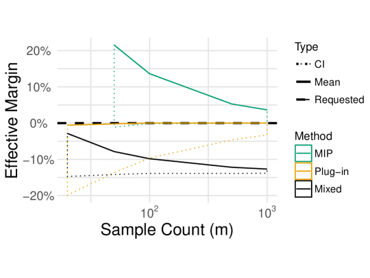
Figure 4: Comparison of margin in probability (MIP) against an A-Basis Value and Plug-In approaches at $\mathcal{R}=0.99$ (Top) and $\mathcal{R}=1-10^{-7}$ (Bottom). The MIP approach is carried out semi-analytically. The MIP results are similar to those of the MIL PM (Fig. 3), but demonstrate the confidently conservative property defined above. Note that at lower sample counts ($m<50$) in the strict reliability case (Bottom), results are not given for low sample counts. This is due to realizations where the estimated margin is incompatible with the desired reliability (i.e. $\mathcal{R}+p>1$) – this strategy is C2 contingent on the constraint $R(\hat{\boldsymbol{\theta}})\geq\mathcal{R}+p$. This pathology illustrates a point: Margin in probability is a more numerically unstable procedure, as compared with other forms of margin suggested in this work. An alternative (positive) view on the phenomenon is that margin in probability can signal that the available information is incompatible with the desired reliability targets. In practice, a designer may use MIP to determine when additional precision in estimates is required.

4 Enabling Estimation

The implementations of PM above are intractable for realistic problems, as they rely on knowledge of the unknown parameters $\boldsymbol{\theta}$, and utilize exact reliability evaluations or expensive second-order Monte Carlo approximations. This section builds up the tools necessary to enable estimation of the two PM implementations introduced above, using only information available through the estimated parameters $\hat{\boldsymbol{\theta}}$ and limit state function evaluations $g(\boldsymbol{d},\boldsymbol{X}_{i}(\hat{\boldsymbol{\theta}}))$. The key insight is to build a random variable model of our margin terms, justified by the delta method and enabled by an efficient gradient approximation technique.

4.1 Delta Method

The delta method is a classical result from the statistics community, and is frequently used to estimate moments and construct confidence intervals.[15] A theorem sufficient for our purposes is stated here.

Theorem: Let $\phi:\mathbb{R}^{d_{p}}\to\mathbb{R}$ be differentiable at $\boldsymbol{\theta}\in\mathbb{R}^{d_{p}}$, and let $\hat{\boldsymbol{\theta}}\sim\mathcal{N}(\boldsymbol{\theta},\boldsymbol{T}_{m})$ be a random vector with $\boldsymbol{T}_{m}\to 0$ as $m\to\infty$. Then $\phi(\hat{\boldsymbol{\theta}})\stackrel{{\scriptstyle d}}{{\to}}\mathcal{N}(\boldsymbol{\theta},\left.\nabla_{\boldsymbol{\theta}}\phi\right|_{\boldsymbol{\theta}}^{\top}\boldsymbol{T}_{m}\left.\nabla_{\boldsymbol{\theta}}\phi\right|_{\boldsymbol{\theta}})$ as $m\to\infty$, where $\stackrel{{\scriptstyle d}}{{\to}}$ denotes convergence in distribution.

The theorem above can be understood in terms of a first-order Taylor approximation to the function $\phi(\hat{\boldsymbol{\theta}})\approx\phi(\boldsymbol{\theta})+\nabla_{\boldsymbol{\theta}}\phi^{\top}(\hat{\boldsymbol{\theta}}-\boldsymbol{\theta})$, which has a mean and variance matrix matching the normal distribution above. As the estimator $\hat{\boldsymbol{\theta}}$ concentrates towards $\boldsymbol{\theta}$ with increasing $m$ (implied by its shrinking covariance matrix), the first-order approximation becomes more accurate, providing an intuitive explanation of the delta method. Note that more general results may be employed for non-normal cases, so long as a similar convergence criterion is met.[15]

Crucially, the result above implies that, under the stated conditions, a function of our estimated parameters $\hat{\boldsymbol{\theta}}$ is asymptotically normal – an implication which we may use to build a model of our margin terms. We will employ plug-in estimates for the parameters ($\boldsymbol{\theta},\boldsymbol{T}$), which leaves the gradient remaining to estimate.

4.2 Parameter Gradients

A simple means to approximate the gradient would be a finite difference approximation. However, this approach would be problematic if the mean difference were approximated via Monte Carlo sampling. For example, if $n$ samples were employed to estimate $g_{MIL,\mathcal{C}}$, an additional $n\times d_{r}$ samples would be required to approximate $\left.\nabla_{\hat{\boldsymbol{\theta}}}g_{MIL,\mathcal{C}}\right|_{\hat{\boldsymbol{\theta}}}$. Furthermore, the computational noise arising from Monte Carlo estimation would necessitate a careful choice of finite difference step size.[16]

Rather than employ finite differences, we leverage the analytic form of the modeled random variable $\rho(\hat{\boldsymbol{\theta}})$ in the likelihood ratio (LR) approach.[9] Note that both the mean difference and probability margins are defined in terms of an expectation; we will first consider the general case, and then specialize the results below.

Let

$$\phi(\hat{\boldsymbol{\theta}}) =\mathbb{E}_{\boldsymbol{X}(\hat{\boldsymbol{\theta}})}[f(\boldsymbol{X}(\hat{\boldsymbol{\theta}}))],$$ (21)

$$=\int f(\boldsymbol{X})\rho(\boldsymbol{X};\hat{\boldsymbol{\theta}})d\boldsymbol{X},$$

and note that $\phi(\hat{\boldsymbol{\theta}})$ depends on its argument only through the distribution PDF; that is, not through $f(\cdot)$ directly. Thus, we may manipulate the gradient

$$\left.\nabla_{\hat{\boldsymbol{\theta}}}\phi\right|_{\hat{\boldsymbol{\theta}}} =\nabla_{\hat{\boldsymbol{\theta}}}\int f(\boldsymbol{X})\rho(\boldsymbol{X};\hat{\boldsymbol{\theta}})d\boldsymbol{X},$$ (22)

$$=\int f(\boldsymbol{X})\nabla_{\hat{\boldsymbol{\theta}}}\rho(\boldsymbol{X};\hat{\boldsymbol{\theta}})d\boldsymbol{X},$$

$$=\int f(\boldsymbol{X})\frac{\nabla_{\hat{\boldsymbol{\theta}}}\rho(\boldsymbol{X};\hat{\boldsymbol{\theta}})}{\rho(\boldsymbol{X};\hat{\boldsymbol{\theta}})}\rho(\boldsymbol{X};\hat{\boldsymbol{\theta}})d\boldsymbol{X},$$

$$=\mathbb{E}_{\boldsymbol{X}(\hat{\boldsymbol{\theta}})}\left[f(\boldsymbol{X})\frac{\nabla_{\hat{\boldsymbol{\theta}}}\rho(\boldsymbol{X};\hat{\boldsymbol{\theta}})}{\rho(\boldsymbol{X};\hat{\boldsymbol{\theta}})}\right],$$

which is an expectation with respect to the same density $\rho(\hat{\boldsymbol{\theta}})$, but with a modified integrand. The quantity $\nabla_{\hat{\boldsymbol{\theta}}}\rho(\boldsymbol{X};\hat{\boldsymbol{\theta}})/\rho(\boldsymbol{X};\hat{\boldsymbol{\theta}})$ is known as the score function.[15] At first, expectation (22) may appear to be a new quantity requiring a separate Monte Carlo estimate, which would double the expense of approximating $\phi(\hat{\boldsymbol{\theta}})$ alone. However, note that $f(\boldsymbol{X})$ is unchanged within the expectation of (22); the parameter sensitivity is represented by the score. If $\phi$ were approximated via Monte Carlo

$$\phi(\hat{\boldsymbol{\theta}})\approx\frac{1}{m}\sum_{i=1}^{m}f(\boldsymbol{X}_{i}(\hat{\boldsymbol{\theta}})),$$ (23)

with $\boldsymbol{X}_{i}(\hat{\boldsymbol{\theta}})\sim\rho(\hat{\boldsymbol{\theta}})$, then we may approximate the gradient using the same samples via

$$\left.\nabla_{\hat{\boldsymbol{\theta}}}\phi\right|_{\hat{\boldsymbol{\theta}}}\approx\frac{1}{m}\sum_{i=1}^{m}f(\boldsymbol{X}_{i}(\hat{\boldsymbol{\theta}}))\frac{\nabla_{\hat{\boldsymbol{\theta}}}\rho(\boldsymbol{X}_{i}(\hat{\boldsymbol{\theta}});\hat{\boldsymbol{\theta}})}{\rho(\boldsymbol{X}_{i}(\hat{\boldsymbol{\theta}});\hat{\boldsymbol{\theta}})}.$$ (24)

Since the evaluation of $f$ is usually the limiting computation, this procedure adds virtually no additional computational expense.

4.3 Modeling the Margin in Limit

The parameter gradient may be employed to model and estimate the margin in limit in an economical fashion. Let

$$D(\boldsymbol{d},\hat{\boldsymbol{\theta}}) =\mathbb{E}_{\boldsymbol{X}(\hat{\boldsymbol{\theta}})}[g(\boldsymbol{d},\boldsymbol{X}(\hat{\boldsymbol{\theta}}))]-\mathbb{E}_{\boldsymbol{X}}[g(\boldsymbol{d},\boldsymbol{X})],$$ (25)

$$=\mathbb{E}_{\boldsymbol{X}(\hat{\boldsymbol{\theta}})}\left[g(\boldsymbol{d},\boldsymbol{X}(\hat{\boldsymbol{\theta}}))-\mathbb{E}_{\boldsymbol{X}}[g(\boldsymbol{d},\boldsymbol{X})]\right],$$

which has the parameter gradient

$$\left.\nabla_{\hat{\boldsymbol{\theta}}}D\right|_{\boldsymbol{d},\hat{\boldsymbol{\theta}}}=\mathbb{E}_{\boldsymbol{X}(\hat{\boldsymbol{\theta}})}\left[\left(g(\boldsymbol{d},\boldsymbol{X}(\hat{\boldsymbol{\theta}}))-\mathbb{E}_{\boldsymbol{X}}[g(\boldsymbol{d},\boldsymbol{X})]\right)\frac{\nabla_{\hat{\boldsymbol{\theta}}}\rho(\hat{\boldsymbol{\theta}})}{\rho(\hat{\boldsymbol{\theta}})}\right],$$ (26)

which enables first-order approximation of the moments

$$\mu_{D}(\boldsymbol{d},\hat{\boldsymbol{\theta}}) \approx\tilde{\mu}_{D}(\boldsymbol{d},\hat{\boldsymbol{\theta}})=0,$$ (27)

$$\tau_{D}(\boldsymbol{d},\hat{\boldsymbol{\theta}})^{2} \approx\tilde{\tau}_{D}(\boldsymbol{d},\hat{\boldsymbol{\theta}})^{2}\equiv\left.\nabla_{\hat{\boldsymbol{\theta}}}D\right|_{\boldsymbol{d},\hat{\boldsymbol{\theta}}}^{\top}\boldsymbol{T}_{m}\left.\nabla_{\hat{\boldsymbol{\theta}}}D\right|_{\boldsymbol{d},\hat{\boldsymbol{\theta}}}.$$

As noted above, in the case where $\hat{\boldsymbol{\theta}}\stackrel{{\scriptstyle d}}{{\to}}\mathcal{N}(\boldsymbol{\theta},\boldsymbol{T}_{m})$, we find that $D(\boldsymbol{d},\hat{\boldsymbol{\theta}})$ is asymptotically normal. This justifies a model for the margin in limit PM

$$\mathbb{P}_{Z}[\tilde{g}_{MIL,\mathcal{C}}>\tilde{\mu}_{D}(\boldsymbol{d},\hat{\boldsymbol{\theta}})+Z\tilde{\tau}_{D}(\boldsymbol{d},\hat{\boldsymbol{\theta}})]=\mathcal{C},$$ (28)

with $Z\sim\mathcal{N}(0,1)$. This model problem has the exact solution

$$\tilde{g}_{MIL,\mathcal{C}}=\Phi^{-1}(\mathcal{C})\tilde{\tau}_{D}(\boldsymbol{d},\hat{\boldsymbol{\theta}}).$$ (29)

Note that in order to evaluate the required moments, we formally require the true value of $\boldsymbol{T}$; in practice, we use a plug-in estimate. Figure 5 compares the MIL PM approximation (using plug-in estimates) against the analytic approach (using true values).

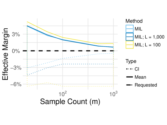
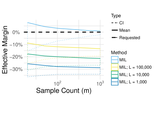
Figure 5: Comparison of approximate and exact margin in limit PM (MIL PM) approaches at $\mathcal{R}=0.99$ (Top) and $\mathcal{R}=1-10^{-7}$ (Bottom). The analytic approach is compared against Monte Carlo approximation using the delta method, varying the number $L$ of Monte Carlo samples. Note that the confidence bounds of the approximation converge on those of the analytic approach, and the approximate mean behavior is quite near the analytic results. Note also that in the high reliability case, the low sample count $L$ leads to highly under-performing designs, in terms of both mean and quantiles. This is due to inaccuracies in both the estimated reliability and margin terms.

4.4 Modeling the Margin in Probability

Much like the margin in limit, we may model and approximate the margin in probability via the delta method. The approach is nearly identical; first define $r=R(\hat{\boldsymbol{\theta}})-R(\boldsymbol{\theta})$, and compute the partials

$$\left.\nabla_{\hat{\boldsymbol{\theta}}}r\right|_{\boldsymbol{d},\hat{\boldsymbol{\theta}}}=\mathbb{E}_{\boldsymbol{X}(\hat{\boldsymbol{\theta}})}\left[\textbf{1}[g(\boldsymbol{d},\boldsymbol{X}(\hat{\boldsymbol{\theta}}))>0]\frac{\nabla_{\hat{\boldsymbol{\theta}}}\rho(\hat{\boldsymbol{\theta}})}{\rho(\hat{\boldsymbol{\theta}})}\right],$$ (30)

where $\textbf{1}[\cdot]$ is the indicator function. Note that $R(\boldsymbol{\theta})$ depends only indirectly upon $\hat{\boldsymbol{\theta}}$, thus it is eliminated in the computation of partials. The gradient above enables first-order approximation of the moments

$$\mu_{r}(\boldsymbol{d},\hat{\boldsymbol{\theta}}) \approx\tilde{\mu}_{r}(\boldsymbol{d},\hat{\boldsymbol{\theta}})=0,$$ (31)

$$\tau_{r}(\boldsymbol{d},\hat{\boldsymbol{\theta}})^{2} \approx\tilde{\tau}_{r}(\boldsymbol{d},\hat{\boldsymbol{\theta}})^{2}\equiv\left.\nabla_{\hat{\boldsymbol{\theta}}}R\right|_{\boldsymbol{d},\hat{\boldsymbol{\theta}}}^{\top}\boldsymbol{T}_{m}\left.\nabla_{\hat{\boldsymbol{\theta}}}R\right|_{\boldsymbol{d},\hat{\boldsymbol{\theta}}},$$

which in turn enable approximation of the probability margin via

$$p\approx\Phi^{-1}(\mathcal{C})\tilde{\tau}_{r}(\boldsymbol{d},\hat{\boldsymbol{\theta}}).$$ (32)

Figure 6 presents results for uniaxial tension using this approximation technique within a Monte Carlo approach, compared against a construction similar to the predictive reliability index (PRI).[4] Der Kiureghian provides an approximation to the PRI $\tilde{\beta}$ based on the delta method to the standard reliability index $\beta(\boldsymbol{\theta})=\Phi^{-1}(R(\boldsymbol{\theta}))$, given by

$$\mu_{\beta} \approx\Phi^{-1}(R(\hat{\boldsymbol{\theta}})),$$ (33)

$$\sigma_{\beta}^{2} =\left.\nabla_{\hat{\boldsymbol{\theta}}}\beta\right|_{\hat{\boldsymbol{\theta}}}^{\top}\hat{\boldsymbol{T}}\left.\nabla_{\hat{\boldsymbol{\theta}}}\beta\right|_{\hat{\boldsymbol{\theta}}},$$

$$\tilde{\beta} =\frac{\mu_{\beta}}{\sqrt{1+\sigma_{\beta}^{2}}}.$$

Note that the PRI formally implies a Bayesian approach, while we have so far employed frequentist constructions. Regardless, we will use the manipulations arising from (33) in the same fashion as the approximations presented above, in order to provide some comparison against existing approaches. Note that we cannot use the approximation technique of Ito et al.,[3] as our design problem does not take the form of design variables perturbed by noise. One designs with the PRI via the constraint $\tilde{\beta}\geq\Phi^{-1}(\mathcal{R})$; we present results from this approach in Figure 6. Note that (33) effectively inflates the variance, but provides no margin to the computed reliability index – Figure 6 demonstrates that the delta-approximated PRI behaves much like the plug-in approach; it is not as conservative as the MIP approach.

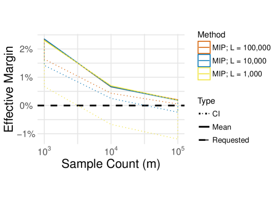
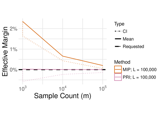
Figure 6: Effective margin for uniaxial tension at $\mathcal{R}=0.90$ using approximate probability margin (Top), and compared against the predictive reliability index (PRI) approach (Bottom). Here we investigate a more lax reliability target, in order to illustrate an important effect: Note that as the sample count increases, the Monte Carlo samples ($L$) must increase to maintain the confidently conservative property. This implies that a higher-accuracy reliability calculation must be used to properly leverage more accurate parameter estimates. Also note that while PRI does account for parameter uncertainties, it is not C2, as it does not add any form of margin. Conspicuously, we do not present a high-reliability case comparison – this is because the MIP formulation is extremely expensive to run using simple Monte Carlo in the high reliability case! We will return to this point in Section 6.

Figure 6 demonstrates that careful balancing of the sample count $m$ and number of Monte Carlo samples $n$ is necessary to approach the C2 property promised by the analytic MIP approach. We perform a scalar analysis (Appendix 7.4) to study this phenomenon, and find that the Monte Carlo estimated variance $\hat{\tau}^{2}$ has variance in excess of $\tilde{\tau}^{2}$ approximated by

$$\mathrm{V}[\hat{\tau}^{2}]\approx\mathrm{V}[\tilde{\tau}^{2}]\left(1+k\frac{m}{n}\right),$$ (34)

where $m$ is the sample count, $n$ is the number of Monte Carlo samples, and $k\in\mathbb{R}_{>0}$ is an unknown constant. Equation 34 illustrates that the estimated margin $\hat{p_{\mathcal{C}}}=\Phi^{-1}(\mathcal{C})\hat{\tau}$ has dispersion in excess of that considered in the delta method. An increase in $m$ must be met with a comparable increase in $n$, in order to combat this deleterious effect.

4.5 Integration and Implementation

Before moving on to our final example, we first discuss the practical integration of PM into a reliability-based design optimization (RBDO) procedure. In order to fully realize the efficiency promised by the approximation techniques above, particular integration choices must be made when implementing the design and analysis loops.

First, since PM may (in general) depend on the design variables $\boldsymbol{d}$, it must be estimated alongside the system reliability. In both the margin in limit and margin in probability approaches we provide $\hat{\boldsymbol{\theta}},\hat{\boldsymbol{T}}$, select $\mathcal{R},\mathcal{C}$, and enforce a modified constraint. In the margin in limit approach, we enforce

$$\mathbb{P}_{\boldsymbol{X}(\hat{\boldsymbol{\theta}})}[g(\boldsymbol{d},\boldsymbol{X}(\hat{\boldsymbol{\theta}}))>g_{MIL,\mathcal{C}}] \geq\mathcal{R},$$ (35)

$$\mathbb{P}_{\boldsymbol{X}(\hat{\boldsymbol{\theta}})}\left[g_{MIL,\mathcal{C}}>\mathbb{E}_{\boldsymbol{X}(\hat{\boldsymbol{\theta}})}[g(\boldsymbol{d},\boldsymbol{X}(\hat{\boldsymbol{\theta}}))]-\mathbb{E}_{\boldsymbol{X}}[g(\boldsymbol{d},\boldsymbol{X})]\right] =\mathcal{C},$$

while in the margin in probability approach, we enforce

$$\mathbb{P}_{\boldsymbol{X}(\hat{\boldsymbol{\theta}})}[g(\boldsymbol{d},\boldsymbol{X}(\hat{\boldsymbol{\theta}}))>0] \geq\mathcal{R}+p,$$ (36)

$$\mathbb{P}_{\hat{\boldsymbol{\theta}}}\left[R(\hat{\boldsymbol{\theta}})>\mathcal{R}+p\right] =\mathcal{C}.$$

In the case where the reliability analysis is nested within an optimization loop, the approach is called bi-level;[17] – confusingly, some authors refer to this nesting as a ‘double loop’. For clarity, we note that in this work we seek to address the statistical double loop; other authors have addressed the bi-level issue.[18] Within a particular reliability analysis at value $\boldsymbol{d}$, we first obtain realizations of the limit state $g(\boldsymbol{d},\boldsymbol{X}_{i}(\hat{\boldsymbol{\theta}}))$, either directly (non-intrusively) or by sampling a constructed surrogate (e.g. via an intrusive procedure). We then use these realizations to compute the margin of choice, which we then apply to the reliability problem. Algorithm 1 illustrates both the margin in limit and margin in probability procedures in pseudocode, using simple Monte Carlo.

Data: $\hat{\boldsymbol{\theta}},\hat{\boldsymbol{T}}_{m}$;$\mathcal{R},\mathcal{C},\epsilon,n$

Result: $\boldsymbol{d}^{*}$

Select $\boldsymbol{d}_{0}$
while $C(\boldsymbol{d}_{j})$ not converged within $\epsilon$ do

       Reliability Analysis
for $i=1:n$ do

             $\boldsymbol{X}_{i}\sim\rho(\hat{\boldsymbol{\theta}})$
$g_{i}\leftarrow g(\boldsymbol{d}_{j},\boldsymbol{X}_{i})$
$\nabla_{\hat{\boldsymbol{\theta}}}D_{i}\leftarrow\frac{g_{i}-\overline{g}}{\rho(\boldsymbol{X}_{i};\hat{\boldsymbol{\theta}})}\nabla_{\hat{\boldsymbol{\theta}}}\rho(\boldsymbol{X}_{i};\hat{\boldsymbol{\theta}})$

       end for

      

      
Margin Computation
$\nabla_{\hat{\boldsymbol{\theta}}}D\leftarrow\frac{1}{n}\sum_{i=1}^{n}\nabla_{\hat{\boldsymbol{\theta}}}D_{i}$
$\tau_{D}^{2}\leftarrow\nabla_{\hat{\boldsymbol{\theta}}}D^{\top}\hat{\boldsymbol{T}}_{m}\nabla_{\hat{\boldsymbol{\theta}}}D$
$g_{MIL,\mathcal{C}}=\Phi^{-1}(\mathcal{C})\sqrt{\tau_{D}^{2}}$
$R(\hat{\boldsymbol{\theta}})\leftarrow\frac{1}{n}\sum_{i=1}^{n}\textbf{1}[g_{i}-g_{MIL,\mathcal{C}}>0]$

      
Design Optimization
Select $\boldsymbol{d}_{j+1}$ such that
Minimize $C(\boldsymbol{d}_{j+1})$
Subject to $R(\hat{\boldsymbol{\theta}})\geq\mathcal{R}$

      
Iterate
$j\leftarrow j+1$

end while

return $\boldsymbol{d}^{*}\leftarrow\boldsymbol{d}_{j}$ Data: $\hat{\boldsymbol{\theta}},\hat{\boldsymbol{T}}_{m}$;$\mathcal{R},\mathcal{C},\epsilon,n$

Result: $\boldsymbol{d}^{*}$

Select $\boldsymbol{d}_{0}$
while $C(\boldsymbol{d}_{j})$ not converged within $\epsilon$ do

       Reliability Analysis
for $i=1:n$ do

             $\boldsymbol{X}_{i}\sim\rho(\hat{\boldsymbol{\theta}})$
$g_{i}\leftarrow g(\boldsymbol{d}_{j},\boldsymbol{X}_{i})$
$\nabla_{\hat{\boldsymbol{\theta}}}R_{i}\leftarrow\frac{\textbf{1}[g_{i}>0]}{\rho(\boldsymbol{X}_{i};\hat{\boldsymbol{\theta}})}\nabla_{\hat{\boldsymbol{\theta}}}\rho(\boldsymbol{X}_{i};\hat{\boldsymbol{\theta}})$

       end for

      

      
Margin Computation
$\nabla_{\hat{\boldsymbol{\theta}}}R\leftarrow\frac{1}{n}\sum_{i=1}^{n}\nabla_{\hat{\boldsymbol{\theta}}}R_{i}$
$\tau_{R}^{2}\leftarrow\nabla_{\hat{\boldsymbol{\theta}}}R^{\top}\hat{\boldsymbol{T}}_{m}\nabla_{\hat{\boldsymbol{\theta}}}R$
$p_{\mathcal{C}}=\Phi^{-1}(\mathcal{C})\sqrt{\tau_{R}^{2}}$
$R(\hat{\boldsymbol{\theta}})\leftarrow\frac{1}{n}\sum_{i=1}^{n}\textbf{1}[g_{i}>0]$

      
Design Optimization
Select $\boldsymbol{d}_{j+1}$ such that
Minimize $C(\boldsymbol{d}_{j+1})$
Subject to $R(\hat{\boldsymbol{\theta}})\geq\mathcal{R}+p_{\mathcal{C}}$

      
Iterate
$j\leftarrow j+1$

end while

return $\boldsymbol{d}^{*}\leftarrow\boldsymbol{d}_{j}$

Algorithm 1 Performing reliability-based design optimization with margin in limit (Left) and probability (Right), using simple Monte Carlo. Here $\textbf{1}[\cdot]$ denotes the indicator function. For brevity, the sample mean $\overline{g}$ is used before it is formally available. The optimization algorithm employed is purposefully not specified to emphasize the generality of the margin algorithms. Note that in both implementations, the margin computation uses information already available from the reliability analysis. Since the evaluation of the limit state $g_{i}$ is commonly the most expensive portion of the analysis, the computation of margin in these approaches adds negligible computational expense.

5 Demonstration: Cantilevered Beam

As a demonstration of the application of precision margin in a reliability-based design optimization, we consider the design of a cantilevered beam [19]. Figure 7 illustrates the problem of a rectangular constant cross-section cantilevered beam subject to a lateral load $H$ and vertical load $V$ at its end. Both loads and the beam’s elastic modulus $E$ and yield strength $Y$ are assumed to be normally distributed as shown in table 2; thus the problem has 4 random variables $\mathbf{X}=[H,V,E,Y]^{\top}$. For this problem, we consider exact knowledge of the load distributions, but estimate distribution parameters for material properties $E$ and $Y$ via sampling. The designer has control over two deterministic variables $\boldsymbol{d}=[w,t]^{\top}$, the width $w$ and the thickness $t$ of the beam. The quantities of interest for this problem include the cross-sectional area of the beam $wt$, as well as the stress and displacement of the beam, which are desired to not exceed the yield strength $Y$ and maximum allowable displacement $D_{0}=2.2535$ inches of the beam.

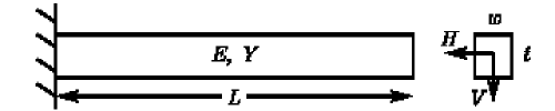
Figure 7: Schematic for the proposed cantilever beam problem subject to a lateral and vertical load [19]. Material properties ($E,Y$) and loading ($H,V$) are uncertain. $L=100$ inches and $w$ and $t$ are deterministic design variables.

Table 2: Truth distributions for the random variables in the cantilevered beam problem.

Name	Variable	Distribution
Lateral load	$H$	$\mathcal{N}(500,100^{2})$
Vertical load	$V$	$\mathcal{N}(1000,100^{2})$
Elastic modulus	$E$	$\mathcal{N}(2.9\times 10^{7},(1.45\times 10^{6})^{2})$
Yield strength	$Y$	$\mathcal{N}(40000,2000^{2})$

The stress $S$, and the displacement $D$ in the beam are given by:

$$S(\boldsymbol{d},\boldsymbol{X})=\frac{600V}{wt^{2}}+\frac{600H}{w^{2}t},$$ (37)

$$D(\boldsymbol{d},\boldsymbol{X})=\frac{4L^{3}}{Ewt}\sqrt{\left(\frac{V}{t^{2}}\right)^{2}+\left(\frac{H}{w^{2}}\right)^{2}},$$ (38)

whereupon the normalized limit state functions $g_{S}$ and $g_{D}$ are written as:

$$g_{S}(\boldsymbol{d},\boldsymbol{X})=1-\frac{S(\boldsymbol{d},\boldsymbol{X})}{Y},$$ (39)

$$g_{D}(\boldsymbol{d},\boldsymbol{X})=1-\frac{D(\boldsymbol{d},\boldsymbol{X})}{D_{0}},$$ (40)

In the MIL implementation, we then formulate and solve the following minimum cross-sectional area (i.e. minimum mass) design problem with chance constraints for the probability of failure to not exceed 0.135%:

min $$C(\boldsymbol{d})=wt,$$ (41)

s.t. $$R_{S}(\hat{\boldsymbol{\theta}})\equiv\mathbb{P}_{\boldsymbol{X}(\hat{\boldsymbol{\theta}})}[g_{S}(\boldsymbol{d},\boldsymbol{X}(\hat{\boldsymbol{\theta}}))>g_{S,MIL,\mathcal{C}}]\geq\mathcal{R}=0.99865,$$

$$R_{D}(\hat{\boldsymbol{\theta}})\equiv\mathbb{P}_{\boldsymbol{X}(\hat{\boldsymbol{\theta}})}[g_{D}(\boldsymbol{d},\boldsymbol{X}(\hat{\boldsymbol{\theta}}))>g_{D,MIL,\mathcal{C}}]\geq\mathcal{R}=0.99865,$$

$$1\leq w,t\leq 4$$

where the limit state margins $g_{S,MIL,\mathcal{C}}$ and $g_{D,MIL,\mathcal{C}}$ defined by the equality constraints in equation 35 calculated for confidence interval $\mathcal{C}=0.95$ are implicit. Similar manipulations yield the MIP approach. In practice, we reformulate the constraints using the performance measure approach by rewriting them using the inverse CDF of the limit state functions [20]. Such a formulation avoids issues during gradient-based optimization when the calculated reliability is 100%.

We compare the results of the reliability-based optimization problem in Figures 8 and 9, and Tables 3 and 4 for several methods: the plug-in approach, mixed approach, and proposed precision margin implementations. We first observe that optimization using the plugin approach leads to designs with an unbiased effective margin which, on average, satisfies the reliability constraints. On the other hand, optimization with basis values leads to excessively conservative designs for this problem, with a large effective margin and extremely high reliability far from the desired value.

In contrast, optimization with the proposed precision margin approaches leads to conservative designs which have positive effective margin and trend towards the desired design reliability with increasing sample count. In particular the delta-approximated margin in probability (MIP) implementation of the precision margin is desirable from an engineering perspective: Although it is not C2 (it is over-conservative), it leads to conservative designs when little information is available about material properties. The approximate MIP approach is able to capitalize on improved information (greater $m$), and approaches true C2 behavior. A comparison of the results in tables 3 and 4 also illustrates the increased effectiveness of the MIP implementation at higher sample counts leading to less conservative but reliable designs.

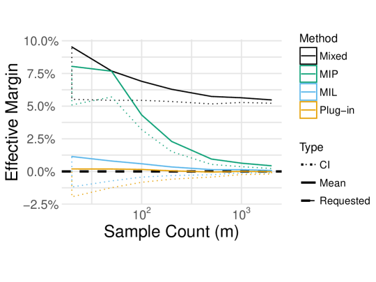
Figure 8: Effective margin for optimal cantilever beam designs using the plug-in approach (PI), basis value approach, and proposed margin in limit (MIL) and margin in probability (MIP) precision margin approaches. Confidence intervals are constructed via a normal approximation from 40 independent optimization results, and chance constraints are estimated via Monte Carlo sampling with $N=1\times 10^{5}$ samples. Note the excessive margin when an A-basis value is used, and improved margin over the plug-in approach when the PM approaches are employed, especially for the margin in probability approach. Note also that the approximate MIP approach is not C2 in this case, as it is somewhat over-conservative, but does approach the theoretical ideal.

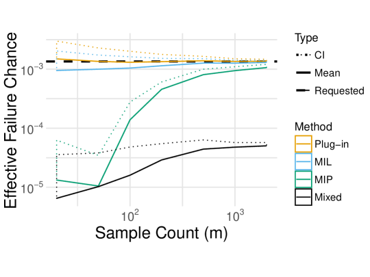
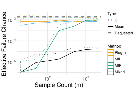
Figure 9: Effective reliabilities with respect to stress (Top) and displacement (Bottom) constraints corresponding to the optimization results shown in figure 8. Optimization with basis values leads to an overly conservative design, whereas design with the precision margin leads to designs with performance closer to the requested performance. In particular, the margin in probability (MIP) PM approach leads to satisfactorily conservative reliabilities which approach the design goal as information about material properties increases.

Table 3: Comparison of cantilever beam optimization results for a sample count of 100 (i.e. using information from 100 material property characterization tests). The average objective (cross-sectional area) value and constraint reliabilities are shown with coefficients of variation in parentheses. For a constant density beam, average weight savings of 2.4% are realized for design using the margin in probability (MIP) PM approach compared to design using basis values (BV). Design using the margin in limit (MIL) PM approach yields average weight savings of 5.9%.

Method	Objective	$\mathbb{E}[t]$	$\mathbb{E}[w]$	$R_{S}$	$R_{D}$
MC+PI	9.53 $(6.02\times 10^{-3})$	3.82	2.49	0.99869 $(4.34\times 10^{-4})$	0.99913 $(3.47\times 10^{-4})$
MC+BV	10.17 $(8.38\times 10^{-3})$	3.90	2.61	0.99998 $(1.98\times 10^{-5})$	0.99999 $(7.23\times 10^{-6})$
MC+MIL PM	9.57 $(6.20\times 10^{-3})$	3.84	2.49	0.99896 $(3.40\times 10^{-4})$	0.99924 $(3.28\times 10^{-4})$
MC+MIP PM	9.93 $(6.63\times 10^{-3})$	3.88	2.56	0.99986 $(8.54\times 10^{-5})$	0.99996 $(1.31\times 10^{-5})$

Table 4: Comparison of cantilever beam optimization results for a sample count of 1000 (i.e. using information from 1000 material property characterization tests). The average objective (cross-sectional area) value and constraint reliabilities are shown with coefficients of variation in parentheses. For a constant density beam, average weight savings of 4.7% are realized for design using the margin in probability (MIP) PM approach compared to design using basis values (BV). Note the increased savings compared to when a sample count of 100 is used. Design using the margin in limit (MIL) PM approach yields average weight savings of 5.2%.

Method	Objective	$\mathbb{E}[t]$	$\mathbb{E}[w]$	$R_{S}$	$R_{D}$
MC+PI	9.51 $(1.47\times 10^{-3})$	3.79	2.51	0.99865 $(9.11\times 10^{-5})$	0.99926 $(1.85\times 10^{-4})$
MC+BV	10.05 $(2.09\times 10^{-3})$	4.00	2.51	0.99995 $(5.77\times 10^{-6})$	0.99996 $(6.75\times 10^{-6})$
MC+MIL PM	9.53 $(1.51\times 10^{-3})$	3.81	2.50	0.99874 $(9.11\times 10^{-5})$	0.99920 $(2.75\times 10^{-4})$
MC+MIP PM	9.58 $(1.69\times 10^{-3})$	3.87	2.48	0.99906 $(9.56\times 10^{-5})$	0.99913 $(2.63\times 10^{-4})$

6 Discussion

In this work, we introduced the concept of precision margin to aid in addressing statistical uncertainties in RBDO. PM is, by construction, capable of controlling a system limit state and avoiding excessive design conservatism. To show the flexibility of this concept, we introduced two operationalizations of the PM concept, introducing margin in limit, and margin in probability. The latter provided an additional benefit: the ability to guarantee a desired reliability at a designed confidence level, what we called confidently conservative (C2). We derived an approximation for and demonstrated the efficacy of both approaches on a classic reliability test case – the cantilever beam problem – which reduced excess weight by $2-5\%$ when compared with design using an A-basis value, while maintaining the desired reliability at (or above) the desired confidence level. This demonstrates the potential of MIP and other PM strategies to produce tangible gains in engineering design for reliability.

Practically, what must be done to perform design for reliability using PM instead of basis values? For the MIP approach suggested above, one must first model the material properties with random variables, in line with existing military design guidelines.[7] One must then estimate the parameters $\hat{\boldsymbol{\theta}}$ for these random variables – this is already done in some approaches to computing basis values.[21] In addition, one must estimate a covariance matrix $\hat{T}_{m}$ for the estimated parameters, for use in the delta method. Finally, one must perform RBDO with MIP as illustrated above; the computational expense of this effort will scale with the desired reliability tolerance, and with the cost involved with system simulation.

Of course, further efforts are necessary to develop and deploy the PM concept. Numerous algorithms and software packages for design for reliability exist, which could benefit from integration with a PM implementation. Acceleration is also key; in this work we considered simple Monte Carlo, which is known to be slow to converge – concretely, this stymied our efforts to apply MIP in the high-reliability case. Integrating PM with fast integrators and quadrature rules is a clear next step. The current implementations of PM suggested here lean heavily on an assumed distribution; this weakness could be lessened by using a more general random variable model, such as the Johnson distribution.[22] Furthermore, it would be desirable to have a non-parametric (empirical) way to implement PM – an approach which would ideally be robust to departures from modeled randomness. An application of the ambiguity set may aid in non-parameteric efforts.[23] Operationally, it may be beneficial to formulate both the design and sampling plan within the same optimization, using margin as a link – recent developments in multi-objective optimization leveraging stochastic dominance appear to be an attractive path forward.[24] Finally, we reiterate that PM is intended to cover statistical uncertainties only – uncertainties addressed by Factors of Safety include unknown unknowns, so a PM could never replace a FOS. However, we believe that precision margin is an early but key component of quantifying, propagating, and above all managing uncertainty in engineering design.

7 Appendix

7.1 Margin in Limit PM

In this entry, we prove that the margin in limit (MIL) approach satisfies convergence property 2. This Appendix entry adopts the more standard statistics notation of Van der Vaart[15], in contrast with the bulk of the manuscript.

Claim: Suppose $\sqrt{m}(\hat{\boldsymbol{\theta}}-\boldsymbol{\theta})\stackrel{{\scriptstyle d}}{{\to}}\mathcal{N}(0,\boldsymbol{T})$. Then the margin $g_{MIL,\mathcal{C}}$ defined in (13) is asymptotically zero, satisfying Point 2.

Pf: Define

$$D(\boldsymbol{d},\hat{\boldsymbol{\theta}})=E_{\boldsymbol{X}(\hat{\boldsymbol{\theta}})}[g(\boldsymbol{d},\boldsymbol{X}(\hat{\boldsymbol{\theta}}))]-\mathbb{E}_{\boldsymbol{X}}[g(\boldsymbol{d},\boldsymbol{X}(\boldsymbol{\theta})),$$ (42)

an application of the delta method [15] yields

$$\sqrt{m}(D(\boldsymbol{d},\hat{\boldsymbol{\theta}})-D(\boldsymbol{d},\boldsymbol{\theta}))\stackrel{{\scriptstyle d}}{{\to}}\mathcal{N}(0,\tau^{\prime 2}),$$ (43)

where $\tau^{\prime 2}=\left.\nabla_{\boldsymbol{\theta}}D\right|_{\boldsymbol{d},\boldsymbol{\theta}}^{\top}\boldsymbol{T}\left.\nabla_{\boldsymbol{\theta}}D\right|_{\boldsymbol{d},\boldsymbol{\theta}}$. Note that $D(\boldsymbol{d},\boldsymbol{\theta})=0$. By the definition of $g_{MIL,\mathcal{C}}$, we have the limit

$$g_{MIL,\mathcal{C}}\to\frac{\tau^{\prime}}{\sqrt{m}}\Phi^{-1}(C),$$ (44)

which completes the proof.$\square$

7.2 Margin in Probability PM

In this entry, we prove that the margin in probability (MIP) approach satisfies convergence property 2.

Claim: Suppose $\sqrt{m}(\hat{\boldsymbol{\theta}}-\boldsymbol{\theta})\stackrel{{\scriptstyle d}}{{\to}}\mathcal{N}(0,\boldsymbol{T})$. Then the margin $p_{\mathcal{C}}$ defined in (13) is asymptotically zero, satisfying Point 2.

Pf: Define

$$r(\boldsymbol{d},\hat{\boldsymbol{\theta}})=R(\boldsymbol{d},\hat{\boldsymbol{\theta}})-R(\boldsymbol{d},\hat{\boldsymbol{\theta}}),$$ (45)

an application of the delta method [15] yields

$$\sqrt{m}(r(\boldsymbol{d},\hat{\boldsymbol{\theta}})-r(\boldsymbol{d},\boldsymbol{\theta}))\stackrel{{\scriptstyle d}}{{\to}}\mathcal{N}(0,\tau^{\prime 2}),$$ (46)

where $\tau^{\prime 2}=\left.\nabla_{\boldsymbol{\theta}}r\right|_{\boldsymbol{d},\boldsymbol{\theta}}^{\top}\boldsymbol{T}\left.\nabla_{\boldsymbol{\theta}}r\right|_{\boldsymbol{d},\boldsymbol{\theta}}$. Note that $r(\boldsymbol{d},\boldsymbol{\theta})=0$. By the definition of $p_{\mathcal{C}}$, we have the limit

$$p_{\mathcal{C}}\to\frac{\tau^{\prime}}{\sqrt{m}}\Phi^{-1}(C),$$ (47)

which completes the proof.$\square$

7.3 Conservative Reliability Index PM

In this entry, we prove that the conservative reliability index (CRI) satisfies convergence property 2.

Claim: Suppose $\sqrt{m}(\hat{\boldsymbol{\theta}}-\boldsymbol{\theta})\stackrel{{\scriptstyle d}}{{\to}}\mathcal{N}(0,\boldsymbol{T})$, and that $R(\hat{\boldsymbol{\theta}})$ is differentiable with respect to $\boldsymbol{\theta}$ at the true parameter value. Then the quantile $R^{\alpha}\to R(\boldsymbol{\theta})$, satisfying Point 2.

Pf: Recall

$$\mathbb{P}_{\hat{\theta}}[R(\hat{\boldsymbol{\theta}})-R^{\alpha}>0]=\alpha,$$ (48)

an application of the delta method [15] to the approximate reliability yields

$$\sqrt{m}(R(\hat{\boldsymbol{\theta}})-R(\boldsymbol{\theta}))\stackrel{{\scriptstyle d}}{{\to}}\mathcal{N}(0,\tau^{\prime 2}),$$ (49)

where $\tau^{\prime 2}=\left.\nabla_{\boldsymbol{\theta}}R\right|_{\boldsymbol{d},\boldsymbol{\theta}}^{\top}\boldsymbol{T}\left.\nabla_{\boldsymbol{\theta}}R\right|_{\boldsymbol{d},\boldsymbol{\theta}}$. The asymptotic solution to auxillary equation (48) is then given by

$$R^{\alpha}\to R(\boldsymbol{\theta})-\frac{\tau^{\prime}}{\sqrt{m}}\Phi^{-1}(\alpha),$$ (50)

thus the constraint $R^{\alpha}\geq\mathcal{R}$ recovers the true reliability constraint $R(\boldsymbol{\theta})\geq\mathcal{R}$ in the asymptotic limit. $\square$

7.4 Balancing Error

In this entry, we study the error contributions to margin in probability using a delta approximation. Suppose we have a single parameter $\theta$, estimated by $t_{m}$, and wish to apply margin $p_{\mathcal{C}}$ of the form

$$\hat{p}_{\mathcal{C}} =\Phi^{-1}(\mathcal{C})\hat{\tau},$$ (51)

$$\hat{\tau}^{2} =\hat{r^{\prime}}t_{m}\hat{r^{\prime}},$$

where $r^{\prime}=\left.\frac{dr}{d\theta}\right|_{t_{m}}$, and $\hat{r^{\prime}}$ is a Monte Carlo approximation of the type described in Section 4.2. Note that $\hat{\tau}^{2}$ is an estimate; thus it is itself randomly distributed. While the delta method guarantees convergence for the estimate $\tilde{\tau}$, it does not account for additional variability arising from the Monte Carlo estimate of the derivative. The following investigation considers the effects of Monte Carlo on $\hat{\tau}^{2}$, compared with $\tilde{\tau}^{2}=t_{m}r^{\prime 2}$.

The central limit theorem endorses the following random variable models

$$t_{m} \sim\mathcal{N}(\theta,\gamma^{2}/m),$$ (52)

$$\hat{r^{\prime}} \sim\mathcal{N}(r^{\prime},\sigma^{2}/n).$$

One may show that $\hat{\tau}^{2}$ has moments given by

$$\mathbb{E}[\hat{\tau}^{2}] =\theta(r^{\prime 2}+\sigma^{2}/n),$$ (53)

$$\mathrm{V}[\hat{\tau}^{2}] =\frac{\gamma^{2}}{m}r^{\prime 4}\left[1+\left(\frac{3}{r^{\prime 4}}+2\frac{\theta^{2}m}{r^{\prime 4}\gamma^{2}}\right)\left(2\frac{\sigma^{2}}{n}r^{\prime 2}+\frac{\sigma^{4}}{n^{2}}\right)\right].$$

The expectation $\mathbb{E}[\hat{\tau}^{2}]$ illustrates bias in our estimate, but it is always positive, and thus only increases conservatism. In the limit $n,m>>1$, we can approximate

$$\mathrm{V}[\hat{\tau}^{2}] \approx\frac{\gamma^{2}}{m}r^{\prime 4}\left[1+4\frac{\theta^{2}\sigma^{2}}{\gamma^{2}r^{\prime 4}}\frac{m}{n}\right],$$ (54)

$$=\mathrm{V}[\tilde{\tau}^{2}]\left(1+k\frac{m}{n}\right).$$

Equation 54 enables us to understand the error properties demonstrated in Figure 6: Compared with the quantity $\tilde{\tau}^{2}$ considered in the delta method, the estimate $\hat{\tau}^{2}$ has excess variance, scaled by the factor $k\frac{m}{n}$. If the sample count $m$ is increased without a comparable increase in Monte Carlo samples $n$, then the excess variance can result in both over- and under-estimated margin terms. It is these under-estimated cases that foil the C2 property of the estimated MIP procedure.

While (54) suggests that ‘balancing’ the sample count $m$ and Monte Carlo samples $n$ is desirable, one cannot make a more precise statement without knowing the value of the constant $k$, which in general will be unknown. A practical heuristic is to seek $m<<n$; fortunately, physical samples $m$ will often be considerably more expensive to gather than computational samples $n$.

7.5 Example: Bias in Reliability Calculation

As mentioned above, the CRI framework of Ito et al.[3] is attractive, but susceptible to bias. Here we provide an example RBDO problem which illustrates this issue. We consider the following problem

min. $$d,$$ (55)

s.t. $$\mathbb{P}_{X(\lambda)}[d-X\geq 0]\geq\mathcal{R},$$

$$d\geq 0,$$

where $\lambda$ parameterizes an exponential random variable $X\sim\text{exp}(1)/\lambda$. In this case $R(\lambda)=1-exp(-\lambda d)$, so $d^{*}=-\log(1-\mathcal{R})/\lambda$. Our objective in this example is to approximate a solution to RBDO problem (55), in the absence of the true value of $\lambda$, but given samples from the true distribution $X_{i}\sim\text{exp}(1)/\lambda$. The maximum likelihood estimator for $\lambda$ is given by

$$\hat{\lambda}=1/\overline{X},$$ (56)

which is known to be biased estimator. While we can easily re-parameterize the exponential distribution to avoid this issue, more generally one may want to work with biased estimators, for instance to take advantage of Stein’s phenomenon.[25]

The original Ito et al. work is framed in terms of failure probabilities, so we carry out the trivial transform to this form, seeking a desired failure probability $\mathcal{F}=1-\mathcal{R}$, and consider the CRI approach

min. $$d,$$ (57)

s.t. $$F^{\alpha}\leq\mathcal{F},$$

$$d\geq 0,$$

$$\mathbb{P}_{\hat{\lambda}}[F(\hat{\lambda})<F^{\alpha}]=\alpha,$$

in comparison with the MIP approach

min. $$d,$$ (58)

s.t. $$F(\hat{\lambda})+p\leq\mathcal{F},$$

$$d\geq 0,$$

$$\mathbb{P}_{\hat{\lambda}}[F(\lambda)-F(\hat{\lambda})<p]=\alpha.$$

Practically, we cannot use the approximation technique suggested in Ito et al.[3], as the shape of the sampling distribution for $\hat{\lambda}$ is dependent on the design variables. We solve both optimization problems semi-analytically, using a monte-carlo approximation for the sampling distribution of $\hat{\lambda}$. We report the single result arising from (57), along with the $\alpha$ -percentile case from (58) in Table 5.

Table 5: Effective margin results from example RBDO problems posed in (57) and (58), with $\mathcal{F}=0.01,\alpha=0.9$, reported against sample count $m$. Note that the CRI approach has an effective margin of nearly $-50\%$ at low sample counts; this is due to the unhandled bias entering through the exponential parameter estimator. The MIP approach achieves an effective margin near machine precision $\epsilon$.

$m$	5	10	25	50	100	500	1000
$M_{eff,CRI}$	$-0.496$	$-0.376$	$-0.239$	$-0.176$	$-0.129$	$-0.058$	$-0.043$
$M_{eff,MIP}$	$O(\epsilon)$	$O(\epsilon)$	$O(\epsilon)$	$O(\epsilon)$	$O(\epsilon)$	$O(\epsilon)$	$O(\epsilon)$

References

- [1] Park Chan Y, Kim Nam H, Haftka Raphael T. How coupon and element tests reduce conservativeness in element failure prediction Reliability Engineering & System Safety. 2014;123:123–136.
- [2] Gelman Andrew, Stern Hal S, Carlin John B, Dunson David B, Vehtari Aki, Rubin Donald B. Bayesian Data Analysis 2013.
- [3] Ito Makoto, Kim Nam Ho, Kogiso Nozomu. Conservative reliability index for epistemic uncertainty in reliability-based design optimization Structural and Multidisciplinary Optimization. 2018;57:1919–1935.
- [4] Der Kiureghian Armen. Analysis of structural reliability under parameter uncertainties Probabilistic engineering mechanics. 2008;23:351–358.
- [5] Noh Yoojeong, Choi KK, Lee Ikjin, Gorsich David, Lamb David. Reliability-based design optimization with confidence level under input model uncertainty in ASME 2009 International Design Engineering Technical Conferences and Computers and Information in Engineering Conference:1121–1136American Society of Mechanical Engineers 2009.
- [6] Kenett Ron, Zacks Shelemyahu. Modern Industrial Statistics Design and Control of Quality and Reliability. Cole Publishing Co., Pacific Grove 1998.
- [7] U.S. Department of Defense . Department of Defense Handbook Polymer Matrix Composites 1997;3. Materials Usage, Design, and Analysis.
- [8] Fonseca José R, Friswell Michael I, Lees Arthur W. Efficient robust design via Monte Carlo sample reweighting International Journal for Numerical Methods in Engineering. 2007;69:2279–2301.
- [9] L’Ecuyer Pierre. A unified view of the IPA, SF, and LR gradient estimation techniques Management Science. 1990;36:1364–1383.
- [10] Li Jinghui, Mosleh Ali, Kang Rui. Likelihood ratio gradient estimation for dynamic reliability applications Reliability Engineering & System Safety. 2011;96:1667–1679.
- [11] Nguyen TH, Song J, Paulino GH. Single-Loop System Reliability Based Design Optimization (SRBDO) Using Matrix-based System Reliability (MSR) Method 2010.
- [12] Bowman K., Cheng L., Chris M., et al. Material qualification and equivalency for polymer matrix composite material systems: Updated procedure 2003.
- [13] Ditlevsen Ove, Madsen Henrik O. Structural reliability methods;178. Wiley New York 1996.
- [14] Meeker William Q, Hahn Gerald J, Escobar Luis A. Statistical intervals: a guide for practitioners and researchers;541. John Wiley & Sons 2017.
- [15] Vaart Aad W.. Asymptotic statistics;3. Cambridge University Press 1998.
- [16] Moré Jorge J, Wild Stefan M. Estimating derivatives of noisy simulations ACM Transactions on Mathematical Software (TOMS). 2012;38:19.
- [17] Eldred Michael, Bichon Barron. Second-order reliability formulations in DAKOTA/UQ in 47th AIAA/ASME/ASCE/AHS/ASC Structures, Structural Dynamics, and Materials Conference 14th AIAA/ASME/AHS Adaptive Structures Conference 7th:1828 2006.
- [18] Agarwal Harish, Renaud John, Lee Jason, Watson Layne. A unilevel method for reliability based design optimization in 45th AIAA/ASME/ASCE/AHS/ASC Structures, Structural Dynamics & Materials Conference:2029 2004.
- [19] Eldred M. S., Agarwal H., Perez V. M., Wojtkiewicz Jr S. F., Renaud J. E.. Investigation of reliability method formulations in DAKOTA/UQ Structure and Infrastructure Engineering. 2007;3:199–213.
- [20] Tu Jian, Choi Kyung K., Park Young H.. A New Study on Reliability-Based Design Optimization ASME Journal of Mechanical Design. 1999;121:557–564.
- [21] Barbero Ever J., Gutierrez Joaquin M.. Determination of basis values from experimental data for fabrics and composites in SAMPE 2012 Conference and Exhibition 2012.
- [22] McDonald Mark, Zaman Kais, Mahadevan Sankaran. Probabilistic Analysis with Sparse Data AIAA Journal. 2013;51:281–290.
- [23] Kapteyn Michael G, Willcox Karen E, Philpott Andy. A Distributionally Robust Approach to Black-Box Optimization in 2018 AIAA Non-Deterministic Approaches Conference:0666 2018.
- [24] Cook Laurence W., Jarrett Jerome P.. Using Stochastic Dominance in Multi-Objective Optimizers for Aerospace Design Under Uncertainty in 2018 AIAA Non-Deterministic Approaches Conference:0665 2018.
- [25] Efron Bradley, Morris Carl. Stein’s paradox in statistics Scientific American. 1977;236:119–127.