Following High-level Navigation Instructions on a Simulated Quadcopter with Imitation Learning

Abstract

We introduce a method for following high-level navigation instructions by mapping directly from images, instructions and pose estimates to continuous low-level velocity commands for real-time control. The Grounded Semantic Mapping Network (GSMN) is a fully-differentiable neural network architecture that builds an explicit semantic map in the world reference frame by incorporating a pinhole camera projection model within the network. The information stored in the map is learned from experience, while the local-to-world transformation is computed explicitly. We train the model using DAggerFM, a modified variant of DAgger that trades tabular convergence guarantees for improved training speed and memory use. We test GSMN in virtual environments on a realistic quadcopter simulator and show that incorporating an explicit mapping and grounding modules allows GSMN to outperform strong neural baselines and almost reach an expert policy performance. Finally, we analyze the learned map representations and show that using an explicit map leads to an interpretable instruction-following model.

I Introduction

Autonomous navigation from high-level instructions requires solving perception, planning and control challenges. Consider the navigation task in Figure 1. To complete the task, a quadcopter must reason about the instruction, observations of the environment, and the sequence of actions to execute. Engineered systems commonly address this challenge using modular architectures connected by curated intermediate representations, including, for example, a perceptual module for object localization, a grounding module to map localization results to the instruction, and a planner to select the trajectory. The required engineering effort is challenging to scale to complex environments. In this paper, we study a learning-based approach to directly predict continuous control commands given an instruction and visual observations. This approach offers multiple benefits, including not requiring explicit design of intermediate representations, implementing planning procedures, or separately training multiple sub-models. We demonstrate the effectiveness of our approach on continuous control of a quadcopter for navigation tasks specified with symbolic instructions.

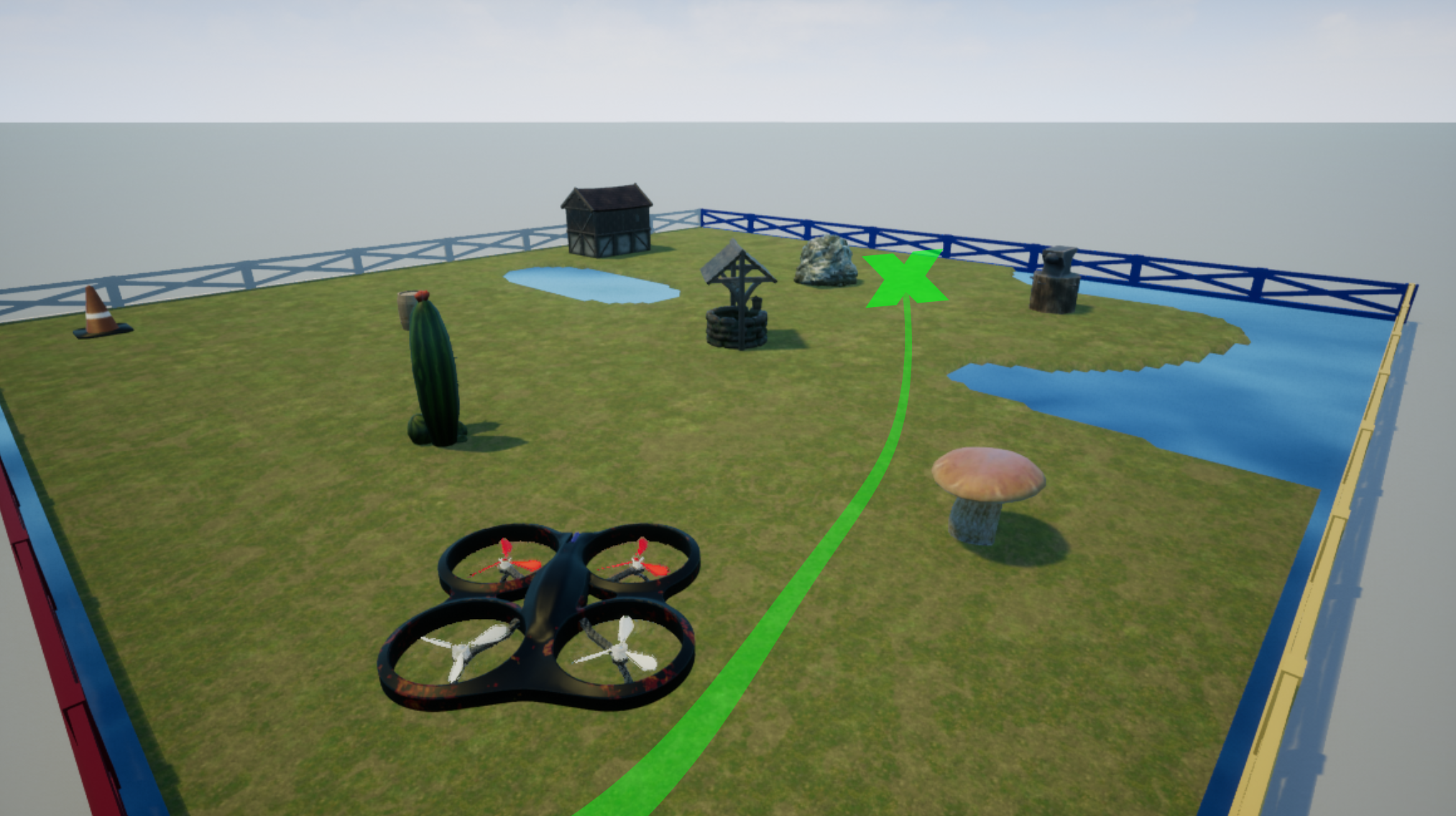
Go to the right side of the rock

Figure 1: High-level instruction in our navigation environment, and an illustration of the goal position and trajectory that the agent must infer and follow given its observations.

Mapping instructions to actions on a quadcopter requires addressing multiple challenges, including building an environment representation by reasoning about observations, recovering the goal from the instruction, and continuous control in a realistic environment. We address these challenges with the Grounded Semantic Mapping Network (GSMN) model (Figure 2). The model consists of a single neural network that explicitly maintains a semantic map by projecting learned features from the agent camera frame into the global reference frame. The map representation is learned from data and can include not only occupancy probabilities, but also high-level semantic information, such as object classes and descriptions. The alignment between the map and the environment enables the agent to accumulate memory of features that disappear from the view and avoid the difficulty of reasoning directly about partially-observed first-person observations.

We train the agent to mimic an expert policy using a variant of DAgger [44]. The flexibility of the model makes learning generalizable representations from instructions, observations, and expert actions challenging. We use a set of auxiliary objectives to help the different parts of the model specialize as expected. For example, we classify the objects mentioned in the instruction from the intermediate map. The auxiliary objectives also solve the credit assignment problem. Any failure can be easily attributed to one of the components, but the entire model is still trained end-to-end, which allows later modules to correct previous mistakes.

We evaluate our approach in a simulated quadcopter environment with language instructions generated from a pre-defined set of templates. Our model is continuously queried and updated at a rate of 5Hz. Our experiments demonstrate that GSMN significantly outperforms standard recurrent architectures that combine convolutional and recurrent layers. Our simulator, code, data, and models are available at https://github.com/clic-lab/gsmn.

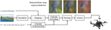
Figure 2: A high-level illustration of the GSMN model. Each block represents a neural network or a deterministic differentiable computation. We overlay the different map representations created on an overhead view of the environment to illustrate how the different maps interpret the various environment elements.

II Technical Overview

II-A Task

We model instruction following as a sequential decision-making process [7]. Let $\mathcal{X}$ be the set of instructions, $\mathcal{S}$ the set of world states, and $\mathcal{A}$ the set of all actions. An instruction $u$ is a sequence of $n$ tokens $\langle u_{1},\dots,u_{n}\rangle$. Given a start state $s_{1}\in\mathcal{S}$ and an instruction $u\in\mathcal{X}$, the agent executes $u$ by generating a sequence of actions, where the last action is the special action ${\tt STOP}$. The agent behavior in the environment is determined by its configuration $c$, which specifies the controller setpoints. Actions deterministically modify the agent configuration or indicate task completion. An execution is an $m$-length sequence $\langle(s_{1},a_{1}),\dots,(s_{m},a_{m})\rangle$, where $s_{j}\in\mathcal{S}$ is the state observed, $a_{j}\in\mathcal{A}$ is the action updating the agent configuration and $a_{m}={\tt STOP}$.

In our navigation task, the agent is a quadcopter flying between landmarks in a simulated 3D environment. The state $s$ specifies the full configuration of the simulator, including the positions of all objects and the quadcopter configuration. The quadcopter location in the environment is given by its pose $P=(p,\theta)$, where $p$ is a position and $\theta$ is an orientation. The quadcopter has a proportional-integral-derivative (PID) flight controller that maintains a fixed altitude, and takes as input the configuration $c$, which consits of two target velocities: linear velocity $v\in\mathds{R}$ and angular yaw-rate $\omega\in\mathds{R}$. An action $a$ is either a tuple $(v,\omega)$ of velocities or the completion action ${\tt STOP}$. Given an action $a_{j}=(v_{j},\omega_{j})$, we set $c_{j}=(v_{j},\omega_{j})$. We observe the environment and generate actions at a fixed rate of 5Hz. The environment simulation runs continuously without interruption. Between actions, the quadcopter configuration is maintained. To correctly complete a task, the agent must take the ${\tt STOP}$ action at the goal position.

II-B Model

The agent observes the environment via a monocular camera sensor, and has access to its location. We distinguish between the world state, which includes the locations of all landmarks and the agent, and the agent context $\tilde{s}$. The agent has access to the agent context only, including for choosing actions. The agent context $\tilde{s}_{j}$ at step $j$ is a tuple $(u,I_{j},P_{j})$, where $u\in\mathcal{X}$ is an instruction, $I_{j}$ is an RGB image, and $P_{j}$ is the agent pose. $I_{j}$ and $P_{j}$ are generated from the current world state $s_{j}$ using the functions $\textsc{Img}(s_{j})$ and $\textsc{Loc}(s_{j})$ respectively. We model the agent using a neural network that explicitly constructs and maintains a semantic map of the environment during execution, and uses the instruction to identify goals in the map. At each step $j$, the network takes as input the agent context $\tilde{s}_{j}$, and predicts the next action $a_{j}$. We formally define the agent and model in Section IV.

II-C Learning

We assume access to a training set of $N$ examples $\{(u^{(i)},s_{1}^{(i)},\Xi^{(i)})\}_{i=1}^{N}$, where $s_{1}^{(i)}$ is a start state, $u^{(i)}$ is an instruction, and $\Xi^{(i)}=\langle P_{1}^{(i)},\dots,P_{m}^{(i)}\rangle$ is a sequence of $m$ poses that defines a trajectory generated by a demonstration execution of $u$. The first pose $P_{1}^{(i)}$ is the quadcopter pose at state $s_{1}^{(i)}$. Given $\Xi^{(i)}$, we design an expert oracle policy using a simple path-following carrot planner tuned to the quadcopter dynamics. During training, for all states, the oracle policy generates actions that move the quadcopter towards and along the demonstration path. We train the agent to mimic the expert policy using a variant of the DAgger [44] algorithm (Section V).

II-D Evaluation

We evaluate task completion error on a test set of $M$ examples $\{(u^{(i)},s^{(i)}_{1},p_{g}^{(i)},r_{g}^{(i)})\}^{M}_{i=1}$, where $u^{(i)}$ is an instruction, $s^{(i)}_{1}$ is a start state, $p_{g}^{(i)}$ is the goal position, and $r_{g}^{(i)}$ is the successful completion region defined by an area surrounding $p_{g}^{(i)}$. We consider a task as completed correctly if the quadcopter takes the ${\tt STOP}$ action inside $r_{g}^{(i)}$ (Section VII).

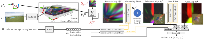
Figure 3: An illustration of our model architecture. The instruction $u$ is encoded with an LSTM network into an instruction embedding at the start of an episode. At each timestep, image features are produced with a custom residual network [ResNet; 14] network and projected on the ground in the global reference frame using a 3D projection based on a pinhole camera model. The projected environment representations are accumulated through time using a masked leaky integration into a persistent map of the world. This map is then filtered to reason about the relevant objects and the most likely goal location using convolutional filters produced from the instruction embedding. From the resulting goal and relevance maps, a dense perceptron (Dense MLP) controller produces a velocity command that drives the robot towards its goal.

III Related Work

Mapping natural language instructions to actions has been studied extensively, both using physical robots [31, 7, 50, 49, 34, 16, 25] and virtual agents [29, 30, 32, 2, 4]. These approaches are based on a modular system architecture, with separate components for language parsing, grounding, mapping, planning, and control. While decomposing the problem, the modular approach requires to explicitly design symbolic intermediate representations, a challenging task for large and complex environments. In contrast, we study a single model-approach using a differentiable model architecture that maps visual observations directly to actions, while learning intermediate representations. This type of approach was studied recently for virtual agents with discrete control [33, 5, 17, 1]. In contrast, we study a continuous control problem using a realistic quadcopter simulator. We follow existing work [5, 17] and abstract the natural language problem by using synthetically generated language. This provides a simple way to specify high-level goals, while focusing our attention on the problem of mapping, planning and task execution.

Recently, using a single differentiable model to map from inputs to outputs across multiple sub-problems has been applied to learning robotic manipulation and control skills [27, 26] and visual navigation in simulated environments [43]. Similar to recent single model instruction following methods [33, 5, 17], these policies are able to learn to effectively complete complex tasks, but suffer from a lack of interpretability. In contrast, we design our model to provide an interpretable view of the agent’s understanding via the semantic map. Our goal is orthogonal to providing safety guarantees [43, 15, 22].

Key to our approach is building a semantic map of the environment within a neural network model. Building environment maps that incorporate information about the semantics of the environment has been studied extensively, commonly with probabilistic graphical models [38, 41, 42, 50, 9]. In contrast, our semantic map is a differentiable 3-axis tensor that is part of a larger neural network architecture and stores a feature vector for every observed location in the world. This approach does not require maintaining a distribution over likely maps. Using a differentiable mapper and planner has been studied for navigation in discrete environments [11, 12, 37, 23]. We work with continuous action and state spaces, and emphasize efficient learning from limited data by incorporating explicit projection and simple aggregation instead of learned memory operations. Including affine transformations and projections inside a neural network has been previously studied in vision and graphics [21, 51]. We use these techniques for learning map-based environment representations.

We evaluate our approach on a realistic simulated quadcopter performing a high-level navigation task. Quadcopters have been recently studied with the goal of learning low-level continuous control [36, 45] or navigation policies [46, 10], where navigation was cast as traversable space prediction using supervised learning. In contrast, we focus on mapping high-level symbolic instructions directly to control signals.

For learning, we use imitation learning [3, 47, 6], where an agent policy is trained to mimick an expert policy while learning how to recover from errors not present in the expert demonstrations. We use a variant of DAgger [44], where states and actions are aggregated from an expert policy for supervised learning. Hussein et al. [20] provides a general overview of imitation learning.

IV Model Architecture

We model the agent policy $\pi$ with a neural network. At time $j$, the input to the policy is the agent context $\tilde{s}_{j}$, and the output is an action $a_{j}$. The action $a_{j}$ modifies the agent configuration $c_{j}$. This process continues until the ${\tt STOP}$ action is predicted and the agent stops. The agent context $\tilde{s}_{j}$ is a tuple $(u,I_{j},P_{j})$, where $u$ is the instruction, $I_{j}=\textsc{Img}(s_{j})$ is the current observation, and $P_{j}=\textsc{Loc}(s_{j})$ is the pose of the agent. Figure 3 illustrates our network architecture.

Our model design incorporates explicit spatial reasoning and memory operations into a differentiable neural network. This relieves the neural network from learning to accomplish complex coordinate transformations that map between the camera and the world reference frame and from learning to integrate current and past observations into a coherent world model. We incorporate a 3D projection and a coordinate frame transformation into our image processing pipeline. Feature representations seamlessly propagate through these operations in a differentiable manner, while the transformations themselves are not learned. The projected image representation is added into a persistent semantic map defined in the global reference frame and aligned with the environment, which allows the agent to easily retain information accumulated through time. This map is similar in principle to the way simultaneous localization and mapping (SLAM) systems store low-level features, such as LIDAR bounces, depth readings or feature descriptors. However, unlike SLAM maps, the features stored are representations learned by our differentiable mapper to directly optimize the task performance.

IV-A Instruction and Image Embedding

We generate representations for both the input text $u$ and the image $I$. We use a recurrent neural network [RNN; 8] with a long short-term memory recurrence [LSTM; 18] to generate a sentence embedding of the input instruction text $\phi_{u}$ by taking the last LSTM output.

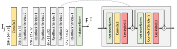
Figure 4: Illustration of our ResNet architecture. The ResNet architecture (left) contains six residual blocks (right). The ResNet has 13 convolutional layers: each block has two convolutional layers and there is one layer at the ResNet input.

Given the observed image $I_{j}$, we compute a feature representation $F^{C}_{j}=\textsc{ResNet}(I_{j})$ using a 13-layer residual convolutional neural network [14] (Figure 4). For a given image $I_{j}$ of size $H\text{x}W\text{x}3$, $F^{C}_{j}$ is a feature map of size $(H/f_{\text{scale}})\text{x}(W/f_{\text{scale}})\text{x}C_{f}$, where the factor $f_{\text{scale}}$ is a hyperparameter of the ResNet. Each pixel in $F^{C}_{j}$ is a feature-vector of $C_{f}$ elements (i.e., channels) that encodes properties of the corresponding image region receptive field. Each pixel in $F^{C}_{j}$ embeds a different image region, which allows recovering locations of objects visible in $I_{j}$ given $F^{C}_{j}$. In our implementation, $C_{f}=32$, $f_{\text{scale}}$ = 8 and the receptive field of each feature vector in $F^{C}_{j}$ is a 61x61 neighborhood in the image $I_{j}$. The resolution of $I_{j}$ is 256x144.

IV-B Feature Projection

The image representation $F^{C}_{j}$ is oriented in the first-person view corresponding to the camera image plane. We project $F^{C}_{j}$ on the ground in the world reference frame to align with the environment and integrate it with previous observations. The current location of each element feature vector $i$ in $F^{C}_{j}$ is represented in homogeneous 2D pixel coordinates as $p^{C}_{i}=[x^{C}_{i},y^{C}_{i},1]^{T}$, where $x^{C}_{i}$ and $y^{C}_{i}$ are the 2D coordinates of $i$ in $F^{C}_{j}$. We use a pinhole camera model to project each element $i$ to the ground in the world reference frame:

$$p^{W}_{i}=T_{C}^{W}\textsc{Raycast}(K^{-1}p^{C}_{i})\mbox{,}$$

where $K$ is the camera matrix, $T_{C}^{W}$ is a camera-to-world affine transformation deterministically computed from the agent pose $P_{j}$, and Raycast is a function that maps a ray to the point where the ray intersects the ground plane at elevation $0$. Poling [40] provides a brief tutorial of camera models. We construct the observation representation $F^{W}_{j}$ in the world reference frame by copying each element $i$ in $F^{C}_{j}$ to the location $p^{W}_{i}$ in $F^{W}_{j}$. To generate the final $F^{W}_{j}$, for each pixel, we interpolate the neighboring points by applying bi-linear interpolation [21]. This creates a discretized tensor representation of $F^{W}_{j}$ and resolve cases where multiple elements are placed in the same pixel location.

IV-C Semantic Map Accumulation

We use the transformed feature map $F^{W}_{j}$ to update a persistent semantic map $S^{W}_{j}$, where we accumulate visual information through time. The map $S^{W}_{j}$ is a 3D tensor with two spatial dimensions and one feature vector dimension to store the different channels generated by the ResNet. Given the feature map $F^{W}_{j}$ computed at step $j$ and the semantic map $S^{W}_{j-1}$ from step $j-1$, we compute the semantic map $S^{W}_{j}$ at step $j$ with a leaky integrator filter:

$$S^{W}_{j}=(1-\lambda)S^{W}_{j-1}+\lambda(F^{W}_{j}\odot M^{W}_{j})+$$

$$\hskip 109.54327pt\lambda(S^{W}_{j-1}\odot(1-M^{W}_{j}))\mbox{,}$$

where $M^{W}_{j}$ is a binary-valued mask indicating which pixels in $S^{W}_{j}$ are within the agent’s field of view and $\odot$ is an element-wise multiplication. This update ensures that (a) unobserved locations (e.g., behind the robot, outside the view of the camera) are not updated, and (b) information is combined with what is already in the map so that an erroneous reading does not fully overwrite valid prior information. The model is able to tolerate moderate amounts of noise in the pose estimate, a likely source of noise in physical robots with GPS or SLAM based localization. We test noise-tolerance in Section VIII.

IV-D Language Grounding and Goal Prediction

We use the instruction embedding $\phi_{u}$ to create two maps from the semantic map: a relevance map that accounts for landmarks mentioned in the instruction and a goal map to identify the goal location. To compute the relevance map, we use the instruction embedding to create a language-dependent 1x1 convolutional filter:

$$\textsc{Conv}_{{\rm label}}=W_{{\rm label}}\phi_{u}+b_{{\rm label}}\mbox{,}$$

where $\phi_{u}$ is the instruction embedding and $W_{{\rm label}}$ and $b_{{\rm label}}$ are learned parameters. The relevance map $R^{W}$ aims to identify the objects in the semantic map mentioned in $u$:

$$R^{W}_{j}=\textsc{Conv}_{{{\rm label}}}(S^{W}_{j})\mbox{.}$$

The goal map $G^{R}$ is computed from the relevance map with wider convolutions to capture spatial relationships. While the relevance map is computed in the global world reference frame, instructions are usually given in the ego-centric agent reference frame. Before computing the goal map, we compute $R^{R}_{j}$ by transforming $R^{W}_{j}$ to the agent reference frame. We use a separate convolution filter computed from the instruction $u$:

$$\textsc{Conv}_{{\rm spatial}}=W_{{\rm spatial}}\phi_{u}+b_{{\rm spatial}}\;\;,$$

where $W_{{\rm spatial}}$ and $b_{{\rm spatial}}$ are learned parameters. $\textsc{Conv}_{{\rm spatial}}$ consists of two cascaded 3x3 convolutions. The goal map is computed as

$$G^{R}_{j}=\textsc{Conv}_{{\rm spatial}}(R^{R}_{j})\;\;.$$

IV-E Control

To compute the output action $a_{j}$, we use a densely-connected two-layer perceptron. Densely connected neural networks have been shown as more stable and faster to train than standard feed-forward models [19]. The input to the perceptron is a concatenation of pre-processed relevance and goal maps and the instruction embedding:

$$\phi_{p_{in}}=[\textsc{ResBlock}_{R}(R^{R}_{j}),\textsc{ResBlock}_{G}(G^{R}_{j}),\phi_{u}]\;\;,$$

where $\textsc{ResBlock}_{(\cdot)}$ is a residual block (Figure 4) with a stride of two to reduce the spatial dimensionality of the maps. Formally, the densely-connected perceptron is:

$$\phi_{p_{1}} = l(W_{p_{1}}\phi_{p_{in}}+b_{p_{1}})\quad$$

$$a_{j} = W_{p_{2}}[\phi_{p_{in}},\phi_{p_{1}}]+b_{p_{2}}\mbox{,}$$

where $l(\cdot)$ is a LeakyReLU activation function [28] and $a_{j}$ is the output action of the policy $\pi$.

IV-F Initial Values and Parameters

At the beginning of execution every element of $S^{W}_{0}$ is set to $\vec{0}$. The model parameters $\Theta$ include the word embeddings used as input for the LSTM, the LSTM, the ResNet, $\textsc{ResBlock}_{R}$, $\textsc{ResBlock}_{G}$ and the matrices and bias vectors: $W_{{\rm label}}$, $W_{{\rm spatial}}$, $W_{p_{1}}$, $W_{p_{2}}$, $b_{{\rm label}}$, $b_{{\rm spatial}}$, $b_{p_{1}}$, $b_{p_{2}}$. The map transformations and observation projections are computed deterministically given the agent pose.

V Learning

We estimate the parameters of the model $\Theta$ using imitation learning with DAggerFM, a variant of DAgger [44] for memory-limited training scenarios. While DAgger provides realistic sample complexity and has been shown to work on robotic agents [45], it requires maintaining an ever-growing dataset to provide stable training. In complex continuous visuo-motor control settings, such as ours, the number of samples generated is large and each sample requires significant amount of memory. This quickly results in exhaustion of memory resources. DAggerFM trades the guarantees of DAgger for a fixed memory budget.

We assume access to a training data of $N$ examples $\{(s_{1}^{(i)},u^{(i)},\Xi^{(i)})\}_{i=1}^{N}$, where $s_{1}^{(i)}$ is a start state, $u^{(i)}$ is an instruction, and $\Xi^{(i)}=\langle P_{1},\dots,P_{m}\rangle$ is a demonstration sequence of $m$ poses starting at $P_{1}^{(i)}=\textsc{Loc}(s_{1}^{(i)})$. Given an expert policy $\pi^{*}$ and a training example $(s_{1}^{(i)},u^{(i)},\Xi^{(i)})$, we minimize the expected distance between the policy actions $a=\pi(\tilde{s})$ and the expert action $a^{*}=\pi^{*}(P,\Xi^{(i)})$. The expectation is computed over the state distribution $d_{\pi}$ induced when executing the learned policy $\pi$ starting from $s_{1}^{(i)}$ and using $u^{(i)}$:

$$J(\Theta)=\mathbb{E}_{s_{j}\sim d_{\pi}}[D_{a}(a,a^{*})]\mbox{.}$$ (1)

During learning, we sample states $s_{j}$ from the state distribution $d_{\hat{\pi}}$ induced by the mixture policy $\hat{\pi}$, which converges to $d_{\pi}$ The distance metric $D_{a}$ is defined as:

$$D_{a}(a,a^{*})= \|v-v^{*}\|^{2}_{2}+\|\omega-\omega^{*}\|^{2}_{2}+$$

$$[p_{{\rm stop}}^{*}log(p_{{\rm stop}})+(1-p_{{\rm stop}}^{*})log(1-p_{{\rm stop}})]\;\;,$$

where $a=(v,\omega,p_{{\rm stop}})$ and $a^{*}=(v^{*},\omega^{*},p_{{\rm stop}}^{*})$. The policy outputs the ${\tt STOP}$ action when $p_{{\rm stop}}>0.5$.

Algorithm 1 shows the training algorithm. Learning begins by collecting a dataset $\mathcal{D}^{*}$ of $N_{s}$ trajectories using the expert policy $\pi^{*}$ for supervised learning. Following supervised training on $\mathcal{D}^{*}$, we sample the initial dataset $\mathcal{D}$ from $\mathcal{D}^{*}$. We then iterate for $K$ iterations. At each iteration, we discard $N_{d}$ trajectories from $\mathcal{D}$, collect new $N_{d}$ trajectories using a mixture policy that interpolates the oracle $\pi^{*}$ and the current policy $\pi_{i}$, update the dataset with the new trajectories, and do one epoch of gradient updates with the aggregated dataset.

DAggerFM does not provide a convergence guarantee for a tabular policy. However, we empirically observe that the dataset performs a stabilizing function similar to that of replay memory in deep Q-learning [35].

$\mathcal{D^{*}}\leftarrow\texttt{collect\_dataset}(\pi^{*},N_{s})$

$\pi_{\theta_{1}}\leftarrow\texttt{train\_supervised}(\mathcal{D^{*}})$

Sample initial dataset $\mathcal{D}\sim\mathcal{D^{*}}$ of size $N$

for $i=1$ to $K$ do

   Discard $N_{d}$ trajectories from $\mathcal{D}$ uniformly at random

   Decay $\beta$: $\beta\leftarrow(\beta_{0})^{i}$

   Let $\hat{\pi}_{i}=\beta\pi^{*}+(1-\beta)\pi_{i}$

   $\mathcal{D}_{i}\leftarrow\texttt{collect\_dataset}(\hat{\pi}_{i},N_{d})$ of size $N_{d}$

   $\mathcal{D}\leftarrow\mathcal{D}\cup\mathcal{D}_{i}$

   $\pi_{i+1}\leftarrow\texttt{train\_epoch}(\mathcal{D},\pi_{i})$ return $\pi_{K}$

Algorithm 1 DAggerFM Training Algorithm for imitation learning with capped dataset size.

VI Auxiliary Objectives

The decomposition of the model architecture according to the different types of expected reasoning (i.e., perception, grounding, and planning) allows us to easily define appropriate auxiliary objectives. These objectives encourage the different parts of the model to assume their intended functions and solve the credit assignment problem. We add four additive auxiliary objectives to the training objective:

$$J(\Theta) = J_{{\rm act}}(\Theta)+\lambda_{v}J_{{\rm percept}}(\Theta)+$$

$$\lambda_{l}J_{{\rm lang}}(\Theta)+\lambda_{g}J_{{\rm ground}}(\Theta)+\lambda_{p}J_{{\rm plan}}(\Theta)\;\;,$$

where $J_{{\rm act}}(\cdot)$ is the main objective (Equation 1) and the four auxiliary objectives are $J_{{\rm percept}}(\cdot)$, $J_{{\rm lang}}(\cdot)$, $J_{{\rm ground}}(\cdot)$, and $J_{{\rm plan}}(\cdot)$. Each auxiliary objective is weighted by a coefficient hyper-parameter.

The perception objective $J_{{\rm percept}}(\cdot)$ aims to require the perception components of the model to correctly classify visible objects. At time $j$, for every object $o$ visible in $I_{j}$, we classify the element in the semantic map $S^{W}_{j}$ corresponding to its location in the world. We apply a linear softmax classifier to every semantic map element that spatially corresponds to the center of an object. The classifier loss is:

$$J_{{\rm percept}}(\Theta)=\frac{-1}{|O_{{\rm FPV}}|}\sum_{o\in O_{{\rm FPV}}}[\hat{y}_{o}log(y_{o})]\;\;,$$

where $\hat{y}_{o}$ is the true class label of the object $o$ and $y_{o}$ is the predicted probability. The instruction objective $J_{{\rm lang}}(\cdot)$ defines a similar objective for the instruction representation. Given an instruction, it requires to classify the object mentioned and the side of the goal (e.g., right, left). The objective is otherwise identical to $J_{{\rm percept}}(\cdot)$.

The grounding and planning objectives $J_{{\rm ground}}(\cdot)$ and $J_{{\rm plan}}(\cdot)$ use binary classification on positions in the relevance and goal maps. Both objectives use a binary cross-entropy loss. The relevance map objective $J_{{\rm ground}}(\cdot)$ classifies each object on the relevance map as to whether it was mentioned in the instruction $u$ or not. For each timestep $j$, we average the objective over all objects in the agent’s field of view. The object mentioned in the instruction is a positive example, and all others are negative examples. The objective is:

$$J_{{\rm ground}}(\Theta)=\frac{-1}{|O_{{\rm FPV}}|}\sum_{o\in O_{{\rm FPV}}}[\hat{y}^{r}_{o}log(y^{r}_{o})+(1-\hat{y}^{r}_{o})log(1-y^{r}_{o})]\mbox{,}$$

where $O_{{\rm FPV}}$ is the set of objects visible from the agent perspective, $\hat{y}^{r}_{o}$ indicates if the object was mentioned in the instruction $u$, and $y^{r}_{o}$ is the prediction of a linear classifier. The goal map objective $J_{{\rm plan}}(\cdot)$ is a similar binary objective, and classifies a point on the goal map as being the goal or not. Positive examples are taken form the annotated goals. For each goal, a negative example is randomly sampled.

VII Experimental Setup

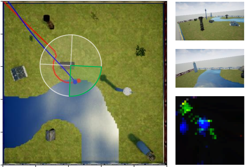
Go to the back side of wooden house

Figure 5: Example environment (left) with 9 objects and an instruction. Ground truth trajectory is shown in red. The trajectory taken by our learned agent policy is in blue. The shaded circle is the target landmark region with $p_{C}-p_{m}<D_{stop}$, and the quadrant highlighted in green is the successful completion region. On the right, from the top: the first observation $I_{0}$, the last observation $I_{37}$, and the final relevance map $R^{W}_{37}$ produced by GSMN model. The relevance map $R^{W}_{37}$ shows the instruction grounding result with both houses highlighted in blue and the wooden house receiving the stronger highlight. The agent correctly stops in the completion region even though the house is outside its field of view in $I_{37}$.

VII-A Environment

We evaluate our approach in randomly generated virtual environments in Unreal Engine. Figure 5 shows an example environment. Each environment consists of a square-shaped green field with edge length of 30 meters and $|O|$ landmarks. We choose $|O|$ uniformly at random between 6 and 13 inclusive and draw landmarks from a pool of 63 3D models without replacement. Landmarks are placed in random locations but no closer than 2.7 meters to the environment edges and at least 1.8 meters apart. We fill the remaining area with random decorative lakes. The quadcopter starts in one of the four corners of the field, facing inwards with a full view of the field. This allows us to validate the model capabilities independently of an exploration strategy.

VII-B Data

For each environment, we randomly sample a pair $\gamma=(\gamma^{C},\gamma^{S})$, where $\gamma^{C}$ is one of the 63 landmarks and $\gamma^{S}$ is one of $\{\textit{left},\textit{right},\textit{front},\textit{back}\}$. Given $\gamma$, we generate the instruction $u$, of the form "go to the $S$ side of $C$", and a goal location $p_{g}$. There are 45 unique noun phrases for the 63 landmarks, and some instructions are ambiguous and unsolvable by even a perfect model. The goal location $p_{g}$ is placed between 2.25 and 3.75 meters from the landmark depending on its size, on the side corresponding to $\gamma_{S}$ when viewed from the start position $p_{0}$. We generate the ground-truth demonstration trajectory $\Xi$ by simulating a point-mass attracted to $p_{g}$ with landmark avoidance constraints. We generate a total of 3500 training, 750 development and 750 testing environments. The same 63 landmarks are found in all dataset splits, but in different combinations and locations. We additionally report results on a pruned test set, where environments with ambiguous instructions have been excluded.

	Success Rate (%)		Distance to Goal (m)
	Overall	Landmark	Mean	Median
GSMN(Ours)	83.47 (87.21)	89.33 (93.38)	2.67 (2.24)	1.21 (1.12)
GSMN w/o $J_{{\rm plan}}$	69.89 (71.03)	84.76 (89.56)	3.19 (2.91)	1.63 (1.65)
GS-FPV	24.93 (27.35)	56.80 (56.03)	7.23 (7.15)	5.14 (4.97)
GS-FPV-MEM	28.67 (33.82)	60.13 (65.74)	6.72 (6.11)	4.34 (3.95)
Oracle (Expert)	87.87 (86.47)	98.40 (98.10)	0.74 (0.78)	0.67 (0.73)
Avg # Steps Fwd	3.32 (3.98)	49.00 (14.12)	11.96 (13.43)	12.23 (13.71)
Random Point	2.13	9.59	15.14	15.05
Random Landmark	17.31	17.31	13.26	13.37

TABLE I: Test results. The numbers in brackets show performance on a pruned version of the test set containing only the 690 environments that do not include ambiguous instructions.

VII-C Evaluation Metric

Given the instruction template $\gamma$, let $p_{C}$ be the location of the target landmark $\gamma^{C}$ in the environment. We define the target landmark region as the circular area where the Euclidean distance of the agent’s last position $p_{m}$ is less than a threshold $D_{stop}$ from $p_{C}$. We subdivide the target landmark region into 4 quadrants, corresponding to left, right, front and back, with respect to the agent’s starting position. We define the task as successfully completed if the agent outputs the action ${\tt STOP}$ within the correct quadrant $r_{g}$ of the target landmark region (see Figure 5). We use $D_{stop}=6\text{ meters}$.

	Success Rate (%)		Dst. to Goal (m)
	Overall	Landmark	Mean	Median
GSMN(Ours)	79.20	86.00	2.98	1.21
GSMN- $J_{{\rm plan}}$	64.40	82.00	3.61	1.75
GSMN- $J_{{\rm ground}}$	5.73	17.73	10.69	10.64
GSMN- $J_{{\rm lang}}$	41.20	57.20	6.62	3.37
GSMN- $J_{{\rm percept}}$	50.00	63.73	5.89	2.55
GSMN+ $\eta_{pos}$	74.40	85.33	3.01	1.41

TABLE II: Development results. We compare our approach against ablations of the different auxiliary objectives and a model that observes noisy poses GSMN+ $\eta_{pos}$.

We additionally report the mean and median of the distance between $p_{m}$ and the ground truth goal position $p_{g}$, as well as the fraction of executions in which the agent stopped in the target landmark region, but on any side of the landmark.

VII-D Systems

We demonstrate the performance of our model GSMN against two neural network baselines that use first-person view: GS-FPV-MEM and GS-FPV. GS-FPV-MEM processes the feature map $F^{C}$ in the first-person view using the same language-derived filters $\textsc{Conv}_{{\rm label}}$ and $\textsc{Conv}_{{\rm spatial}}$ and applies the same auxiliary objectives to all intermediate representations, resulting in per-timestep relevance and goal maps $R^{C}$ and $G^{C}$ in the first-person view. The only difference is that no 3D projection takes place and consequently no environment map is built. Since GSMN uses the semantic map as spatial memory, GS-FPV-MEM uses an LSTM memory cell for this purpose [17, 5]. We store the current $R^{C}$ and $G^{C}$ in the LSTM cell and take the current output of the LSTM as an additional input to the DenseMLP. GS-FPV is a baseline with the same architecture as GS-FPV-MEM, but without the LSTM memory. We do not use $J_{{\rm plan}}$ with the baselines because the goal location may not be visible in view. The direct comparison should be made against the GSMN w/o $J_{{\rm plan}}$ ablation, which uses the the same set of auxiliary objectives.

We use GS-FPV and GS-FPV-MEM as baselines to clearly quantify the contribution of the semantic mapping mechanism. We also compare against three trivial baseline models: (a) take the average action for average number of steps (30); (b) go to a random point in the field; and (c) go to the correct side of a random landmark in the field. As an upper bound, we compare against the expert policy.

Finally, we study the sensitivity of our model to simple noise in the position estimate by adding Guassian noise. We consider the pose at time $j$ as a 3D position and 3D Euler angles $P_{j}=[p_{x},p_{y},p_{z},\theta_{x},\theta_{y},\theta_{z}]$. At each timestep $j$, we replace the pose $P_{j}$ with $\hat{P_{j}}=P_{j}+\eta_{j}$, where $\eta_{j}=[\eta_{p_{x}},\eta_{p_{y}},\eta_{p_{z}},0,0,0]$ is additive noise. Each noise component $\eta_{p_{(\cdot)}}$ is drawn at every timestep $j$ independently at random from a Gaussian distribution with zero mean and variance of 0.5 meters.

VII-E Hyper-parameters and Implementation Details

We train all neural network models using the same procedure. We collect a supervised dataset $\mathcal{D}^{*}$ consisting of sequences of observations and actions on all 3500 training environments by executing the expert policy. We then train on $\mathcal{D}^{*}$ for 30 epochs, and execute DAggerFM for $100$ epochs with $N_{D}=520$ and $M=20$ (Section V). We optimize the parameters $\Theta$ of the policy $\pi$ using ADAM [24] with $\alpha=0.001$, learning rate of $0.001$, L2 regularization with $\gamma=10^{-6}$, and the gradient $\frac{\partial J(\pi)}{\Theta}$. We set $\lambda_{v}$, $\lambda_{g}$, $\lambda_{l}$, and $\lambda_{p}$ to 0.1. We execute the trained policies and baselines on a simulated quadcopter using the Microsoft AirSim [48] plugin for Unreal Engine 4.18, which captures realistic flight dynamics. We control the quadcopter by sending velocity commands to the flight controller in its local reference frame, and limit the linear velocity to 1.6 m/s and the angular velocity to 2.44 rad/s.

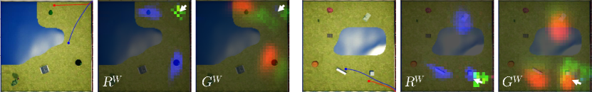
Go to the right side of fir tree Go to the left side of box

Figure 6: Two task failures using our approach. The ground truth and policy trajectories are shown in red and blue respectively. On the left, the failure is due to an ambiguous instruction. The Relevance Map $R^{W}$ overlaid on the environment reveals that the agent has correctly grounded the instruction to the two fir trees present, while ignoring the other objects. The goal map $G^{W}$ shows that the goal location is inferred for both fir trees. The agent correctly reasons about the task, but the ambiguity confuses it. On the right, box is incorrectly grounded to multiple objects as seen in $R^{W}$. Given this wrong grounding, the goal location is inferred to the correct side (left) of all grounded objects, as shown in $G^{W}$. The agent then executes given the confused goal map, which causes it to fly through the correct goal and towards one of the wrongly detected goals.

Figure 7: Accuracy curves for main objective ($J_{{\rm act}}(\cdot)$) and the different auxiliary objectives: perception ($J_{{\rm percept}}(\cdot)$), instruction understanding ($J_{{\rm lang}}(\cdot)$), grounding ($J_{{\rm ground}}(\cdot)$), and planning ($J_{{\rm ground}}(\cdot)$). The curves show the progress of learning in terms of individual accuracies during supervised pre-training measured on the development set. We show the curves for GSMN (left) and GS-FPV-MEM (right).

VIII Results

Table I shows our test results. Our approach significantly outperforms the baselines. While our full approach includes the goal auxiliary objectives, which the baselines do not have access to, we observe that GSMN w/o $J_{{\rm plan}}$, which ablates this auxiliary objective, also outperforms the RNN baseline GS-FPV-MEM. Our full model GSMN performs very closely to the expert policy, especially when removing ambiguous instructions. In general, the oracle performs imperfectly due to the simple model we use. For example, at times, the agent reaches the goal position in high speed and ends up stopping just outside the correct completion boundary.

Table II shows development results. We ablate each auxiliary objective. Each objective contributes to the model performance. We observe that the grounding objective $J_{{\rm ground}}$ is essential and without it the model fails to learn. The planning auxiliary objective $J_{{\rm plan}}$ is the least important. This suggests that after having successful grounding results, the set of simple spatial relations we use is relatively easy to learn. We also observe that our model is robust to moderate amount of localization noise without a significant decline in performance. This indicates the model potential for physical robotic systems, where position estimates are likely to be noisy.

Figure 7 shows development accuracy of auxiliary objectives during training as function of the number of epochs. We observe that most auxiliary objectives converge for both the GSMN model and the GS-FPV-MEM baseline. The instruction landmark accuracy converges to a relatively low value due to instruction ambiguity.

Our model enables us to easily visualize the agent perception and interpret the cause of errors. Figure 6 shows the visual process we can use to identify if the perception, grounding, planning, or control components failed.

IX Discussion

Neural network architectures have achieved remarkable performance in various high-level tasks, but their applications to the robotics domain have largely been limited to single, repeated tasks [26, 10, 36] or required substantial amount of training data due to high sample-complexity [39].

We show that a modular neural network architecture that (a) assigns explicit roles to its subcomponents in the form of auxiliary objectives; and (b) relieves the neural network from having to learn spatial transformations or memory operations that can be computed explicitly, can obtain strong performance on a complex visual navigation task that requires effective perception, symbol grounding, planning, and control. The model is able to learn from limited amount of data, and generalize to unseen environments. Key to enabling this efficient learning is the combination of auxiliary objectives and a modular architecture that results in explicitly solving the symbol grounding problem [13] by spatial reasoning on a high-level map representation.

There are several directions for future work that follow up on limitations of our model and setup. A key problem that is not addressed by our experiments is exploration. The wide field-of-view provided to the agent abstracts away issues of observability, and allows us to to focus on spatial reasoning and task-completion abilities. While the architecture is not specifically designed for fully observable environments, it is likely that the learning procedure will not be robust to such challenges. A second potential direction for future work is removing the auxiliary objectives. These objectives require ground truth labels of landmarks in the environment and meaning of the instruction. This type of information is challenging to obtain in physical environments or when using natural language instructions.

References

- Anderson et al. [2018] Peter Anderson, Qi Wu, Damien Teney, Jake Bruce, Mark Johnson, Niko Sünderhauf, Ian Reid, Stephen Gould, and Anton van den Hengel. Vision-and-language navigation: Interpreting visually-grounded navigation instructions in real environments. In Proceedings of the IEEE Conference on Computer Vision and Pattern Recognition (CVPR), 2018.
- Artzi and Zettlemoyer [2013] Yoav Artzi and Luke Zettlemoyer. Weakly supervised learning of semantic parsers for mapping instructions to actions. Transactions of the Association for Computational Linguistics, 1(1):49–62, 2013.
- Bakker and Kuniyoshi [1996] Paul Bakker and Yasuo Kuniyoshi. Robot see, robot do: An overview of robot imitation. In AISB96 Workshop on Learning in Robots and Animals, pages 3–11, 1996.
- Branavan et al. [2010] S. R. K. Branavan, Luke S. Zettlemoyer, and Regina Barzilay. Reading between the lines: Learning to map high-level instructions to commands. In Proceedings of the 48th Annual Meeting of the Association for Computational Linguistics, ACL ’10, pages 1268–1277, Stroudsburg, PA, USA, 2010. Association for Computational Linguistics. URL http://dl.acm.org/citation.cfm?id=1858681.1858810.
- Chaplot et al. [2017] Devendra Singh Chaplot, Kanthashree Mysore Sathyendra, Rama Kumar Pasumarthi, Dheeraj Rajagopal, and Ruslan Salakhutdinov. Gated-attention architectures for task-oriented language grounding. CoRR, abs/1706.07230, 2017.
- Daumé III et al. [2009] Hal Daumé III, John Langford, and Daniel Marcu. Search-based structured prediction. 2009. URL http://pub.hal3.name/#daume06searn.
- Duvallet et al. [2013] Felix Duvallet, Thomas Kollar, and Anthony Stentz. Imitation learning for natural language direction following through unknown environments. In Robotics and Automation (ICRA), 2013 IEEE International Conference on, pages 1047–1053. IEEE, 2013.
- Elman [1990] Jeffrey L. Elman. Finding structure in time. Cognitive Science, 14:179–211, 1990.
- Espinace et al. [2013] Pablo Espinace, Thomas Kollar, Nicholas Roy, and Alvaro Soto. Indoor scene recognition by a mobile robot through adaptive object detection. Robotics and Autonomous Systems, 61(9):932–947, 2013.
- Giusti et al. [2016] Alessandro Giusti, Jérôme Guzzi, Dan C Cireşan, Fang-Lin He, Juan P Rodríguez, Flavio Fontana, Matthias Faessler, Christian Forster, Jürgen Schmidhuber, Gianni Di Caro, et al. A machine learning approach to visual perception of forest trails for mobile robots. IEEE Robotics and Automation Letters, 1(2):661–667, 2016.
- Gupta et al. [2017a] Saurabh Gupta, James Davidson, Sergey Levine, Rahul Sukthankar, and Jitendra Malik. Cognitive mapping and planning for visual navigation. In Proceedings of the IEEE Conference on Computer Vision and Pattern Recognition, 2017a.
- Gupta et al. [2017b] Saurabh Gupta, David Fouhey, Sergey Levine, and Jitendra Malik. Unifying map and landmark based representations for visual navigation. arXiv preprint arXiv:1712.08125, 2017b.
- Harnad [1990] Stevan Harnad. The symbol grounding problem. Physica D: Nonlinear Phenomena, 42(1-3):335–346, 1990.
- He et al. [2016] Kaiming He, Xiangyu Zhang, Shaoqing Ren, and Jian Sun. Deep residual learning for image recognition. In Proceedings of the IEEE conference on computer vision and pattern recognition, pages 770–778, 2016.
- Held et al. [2017] David Held, Zoe McCarthy, Michael Zhang, Fred Shentu, and Pieter Abbeel. Probabilistically safe policy transfer. In Robotics and Automation (ICRA), 2017 IEEE International Conference on, pages 5798–5805. IEEE, 2017.
- Hemachandra et al. [2015] Sachithra Hemachandra, Felix Duvallet, Thomas M Howard, Nicholas Roy, Anthony Stentz, and Matthew R Walter. Learning models for following natural language directions in unknown environments. In Robotics and Automation (ICRA), 2015 IEEE International Conference on, pages 5608–5615. IEEE, 2015.
- Hermann et al. [2017] Karl Moritz Hermann, Felix Hill, Simon Green, Fumin Wang, Ryan Faulkner, Hubert Soyer, David Szepesvari, Wojtek Czarnecki, Max Jaderberg, Denis Teplyashin, et al. Grounded language learning in a simulated 3d world. arXiv preprint arXiv:1706.06551, 2017.
- Hochreiter and Schmidhuber [1997] Sepp Hochreiter and Jürgen Schmidhuber. Long short-term memory. Neural computation, 9(8):1735–1780, 1997.
- Huang et al. [2017] Gao Huang, Zhuang Liu, Laurens van der Maaten, and Kilian Q Weinberger. Densely connected convolutional networks. In Proceedings of the IEEE Conference on Computer Vision and Pattern Recognition, 2017.
- Hussein et al. [2017] Ahmed Hussein, Mohamed Medhat Gaber, Eyad Elyan, and Chrisina Jayne. Imitation learning: A survey of learning methods. ACM Comput. Surv., 50(2):21:1–21:35, April 2017. ISSN 0360-0300. doi: 10.1145/3054912. URL http://doi.acm.org/10.1145/3054912.
- Jaderberg et al. [2015] Max Jaderberg, Karen Simonyan, Andrew Zisserman, et al. Spatial transformer networks. In Advances in neural information processing systems, pages 2017–2025, 2015.
- Kahn et al. [2017] Gregory Kahn, Tianhao Zhang, Sergey Levine, and Pieter Abbeel. Plato: Policy learning using adaptive trajectory optimization. In Robotics and Automation (ICRA), 2017 IEEE International Conference on, pages 3342–3349. IEEE, 2017.
- Khan et al. [2018] Arbaaz Khan, Clark Zhang, Nikolay Atanasov, Konstantinos Karydis, Vijay Kumar, and Daniel D. Lee. Memory augmented control networks. In International Conference on Learning Representations, 2018. URL https://openreview.net/forum?id=HyfHgI6aW.
- Kingma and Ba [2015] Diederik P Kingma and Jimmy Ba. Adam: A method for stochastic optimization. The International Conference on Learning Representations (ICLR), 2015.
- Knepper et al. [2015] Ross A Knepper, Stefanie Tellex, Adrian Li, Nicholas Roy, and Daniela Rus. Recovering from Failure by Asking for Help. Autonomous Robots, pages 1–16, 2015.
- Levine et al. [2016a] Sergey Levine, Chelsea Finn, Trevor Darrell, and Pieter Abbeel. End-to-end training of deep visuomotor policies. The Journal of Machine Learning Research, 17(1):1334–1373, 2016a.
- Levine et al. [2016b] Sergey Levine, Peter Pastor, Alex Krizhevsky, and Deirdre Quillen. Learning hand-eye coordination for robotic grasping with large-scale data collection. In International Symposium on Experimental Robotics, pages 173–184. Springer, 2016b.
- Maas et al. [2013] Andrew L Maas, Awni Y Hannun, and Andrew Y Ng. Rectifier nonlinearities improve neural network acoustic models. In Proc. icml, volume 30, page 3, 2013.
- MacMahon et al. [2006] Matt MacMahon, Brian Stankiewicz, and Benjamin Kuipers. Walk the talk: Connecting language, knowledge, and action in route instructions. Def, 2(6):4, 2006.
- Matuszek et al. [2010] Cynthia Matuszek, Dieter Fox, and Karl Koscher. Following directions using statistical machine translation. In Human-Robot Interaction (HRI), 2010 5th ACM/IEEE International Conference on, pages 251–258. IEEE, 2010.
- Matuszek* et al. [2012] Cynthia Matuszek*, Nicholas FitzGerald*, Luke Zettlemoyer, Liefeng Bo, and Dieter Fox. A Joint Model of Language and Perception for Grounded Attribute Learning. In Proc. of the 2012 International Conference on Machine Learning, Edinburgh, Scotland, June 2012.
- Matuszek et al. [2012] Cynthia Matuszek, Evan Herbst, Luke Zettlemoyer, and Dieter Fox. Learning to parse natural language commands to a robot control system. In Proc. of the 13th International Symposium on Experimental Robotics (ISER), June 2012.
- Misra et al. [2017] Dipendra Misra, John Langford, and Yoav Artzi. Mapping instructions and visual observations to actions with reinforcement learning. In Proceedings of the 2017 Conference on Empirical Methods in Natural Language Processing, pages 1015–1026. Association for Computational Linguistics, 2017. URL http://aclweb.org/anthology/D17-1107.
- Misra et al. [2014] Dipendra K Misra, Jaeyong Sung, Kevin Lee, and Ashutosh Saxena. Tell me dave: Context-sensitive grounding of natural language to mobile manipulation instructions. In Robotics: Science and Systems (RSS), 2014.
- Mnih et al. [2015] Volodymyr Mnih, Koray Kavukcuoglu, David Silver, Andrei A Rusu, Joel Veness, Marc G Bellemare, Alex Graves, Martin Riedmiller, Andreas K Fidjeland, Georg Ostrovski, et al. Human-level control through deep reinforcement learning. Nature, 518(7540):529, 2015.
- Mueller et al. [2017] Matthias Mueller, Vincent Casser, Neil Smith, and Bernard Ghanem. Teaching uavs to race using ue4sim. arXiv preprint arXiv:1708.05884, 2017.
- Parisotto and Salakhutdinov [2018] Emilio Parisotto and Ruslan Salakhutdinov. Neural map: Structured memory for deep reinforcement learning. In International Conference on Learning Representations, 2018. URL https://openreview.net/forum?id=Bk9zbyZCZ.
- Persson et al. [2007] Martin Persson, Tom Duckett, Christoffer Valgren, and Achim Lilienthal. Probabilistic semantic mapping with a virtual sensor for building/nature detection. In Computational Intelligence in Robotics and Automation, 2007. CIRA 2007. International Symposium on, pages 236–242. IEEE, 2007.
- Pinto and Gupta [2016] Lerrel Pinto and Abhinav Gupta. Supersizing self-supervision: Learning to grasp from 50k tries and 700 robot hours. 2016 IEEE International Conference on Robotics and Automation (ICRA), pages 3406–3413, 2016.
- Poling [2015] Bryan Poling. A tutorial on camera models. University of Minnesota, pages 1–10, 2015.
- Pronobis [2011] Andrzej Pronobis. Semantic mapping with mobile robots. PhD thesis, KTH Royal Institute of Technology, 2011.
- Pronobis and Jensfelt [2012] Andrzej Pronobis and Patric Jensfelt. Large-scale semantic mapping and reasoning with heterogeneous modalities. In Robotics and Automation (ICRA), 2012 IEEE International Conference on, pages 3515–3522. IEEE, 2012.
- Richter and Roy [2017] Charles Richter and Nicholas Roy. Safe visual navigation via deep learning and novelty detection. In Proc. of the Robotics: Science and Systems Conference, 2017.
- Ross et al. [2011] Stéphane Ross, Geoffrey Gordon, and Drew Bagnell. A reduction of imitation learning and structured prediction to no-regret online learning. In Proceedings of the fourteenth international conference on artificial intelligence and statistics, pages 627–635, 2011.
- Ross et al. [2013] Stéphane Ross, Narek Melik-Barkhudarov, Kumar Shaurya Shankar, Andreas Wendel, Debadeepta Dey, J Andrew Bagnell, and Martial Hebert. Learning monocular reactive uav control in cluttered natural environments. In Robotics and Automation (ICRA), 2013 IEEE International Conference on, pages 1765–1772. IEEE, 2013.
- Sadeghi and Levine [2017] Fereshteh Sadeghi and Sergey Levine. Cad2rl: Real single-image flight without a single real image. In Robotics: Science and Systems (RSS), 2017.
- Schaal et al. [2003] Stefan Schaal, Auke Ijspeert, and Aude Billard. Computational approaches to motor learning by imitation. Philosophical Transactions of the Royal Society B: Biological Sciences, 358(1431):537–547, 2003.
- Shah et al. [2017] Shital Shah, Debadeepta Dey, Chris Lovett, and Ashish Kapoor. Airsim: High-fidelity visual and physical simulation for autonomous vehicles. In Field and Service Robotics, 2017. URL https://arxiv.org/abs/1705.05065.
- Tellex et al. [2011] Stefanie Tellex, Thomas Kollar, Steven Dickerson, Matthew R Walter, Ashis Gopal Banerjee, Seth Teller, and Nicholas Roy. Approaching the Symbol Grounding Problem with Probabilistic Graphical Models. AI Magazine, 32(4):64, 2011.
- Walter et al. [2013] Matthew R Walter, Sachithra Hemachandra, Bianca Homberg, Stefanie Tellex, and Seth Teller. Learning Semantic Maps from Natural Language Descriptions. In Robotics: Science and Systems, 2013.
- Yan et al. [2016] Xinchen Yan, Jimei Yang, Ersin Yumer, Yijie Guo, and Honglak Lee. Perspective transformer nets: Learning single-view 3d object reconstruction without 3d supervision. In Advances in Neural Information Processing Systems, pages 1696–1704, 2016.
- Yu and Koltun [2016] Fisher Yu and Vladlen Koltun. Multi-scale context aggregation by dilated convolutions. In ICLR, 2016.