$\eta$-${}^{4}{\rm He}$ interaction from the $dd\to\eta^{4}{\rm He}$ reaction near threshold

Abstract

We analyze the data on the total cross sections for the $dd\to\eta{}^{4}{\rm He}$ reaction close to threshold and look for possible $\eta^{4}{\rm He}$ bound states. We develop a framework in which the $\eta^{4}{\rm He}$ optical potential is the key ingredient, rather than parameterizing the scattering matrix, as is usually done. The strength of this potential, together with some production parameters, are fitted to the available experimental data. The relationship of the scattering matrix to the optical potential is established using the Bethe-Salpeter equation and the $\eta^{4}{\rm He}$ loop function incorporates the range of the interaction given by the experimental ${}^{4}{\rm He}$ density. However, when we look for poles of the scattering matrix, we get poles in the bound region, poles in the positive energy region or no poles at all. If we further restrict the results with constraints from a theoretical model with all its uncertainties the bound states are not allowed. However, we find a bump structure in $|T|^{2}$ of the $\eta^{4}{\rm He}\to\eta^{4}{\rm He}$ amplitude below threshold for the remaining solutions.

I Introduction

The search for $\eta$ bound states in nuclei has been a constant thought for several years Wilkin:2016ajz ; Bass:2015ova ; Haider:2015fea ; Kelkar:2015bta ; Hirenzaki:2015eoa ; Friedman:2013zfa , starting from the early works of Refs. Bhaleliu ; Haiderliu ; Liuhaider . Follow up evaluations of the $\eta$-nucleus optical potential, with special attention to two-nucleon $\eta$ absorption, showed that, while indeed the $\eta N$ interaction was strong enough to bind $\eta$ states, the widths were always bigger than the binding chiang .

The $\eta$-nucleus interaction within the chiral unitary approach was studied in Ref. Inoueta , where enough attraction was found to form bound $\eta$-nucleus states. Detailed studies of the $\eta$ energies for different nuclei were made in Ref. GarciaRecio:2002cu where, for medium and light nuclei, bound states were found (see also Ref. Cieply:2013sga , where qualitatively similar conclusions were drawn), though with larger widths than binding energies. For instance, some theoretical calculations for light systems predicted binding energy $B_{E}$ of around 1 MeV or less and width $\Gamma=15$ MeV for $\eta^{3}{\rm He}$ Barnea:2015lia . In the recent work Barnea:2017oyk the results of Ref. Barnea:2015lia have been updated, in particular the new width is much smaller. In Ref. Xie:2016zhs , the data on cross sections and asymmetries for the $pd\to\eta{}^{3}{\rm He}$ reaction close to threshold were studied with the aim of looking for bound states of the $\eta^{3}{\rm He}$ system. The resulting $\eta^{3}{\rm He}$ scattering matrix had a local Breit-Wigner form in a narrow range of energies which corresponded to a binding of about $0.3$ MeV and a width of about $3$ MeV. However, the pole appeared in the continuum, not in the bound region.

The fact that the widths are expected to be much larger than the binding might be the reason why so far, we have no conclusive evidence for any of these bound states Bilger:2002aw ; Mersmann ; Colin ; Rausmann:2009dn ; Urban:2009zzc ; Chrien:1988gn ; Johnson:1993zy ; Frascaria:1994va ; Willis:1997ix ; Wronska:2005wk ; Skurzok:2011aa ; Adlarson:2013xg ; Krzemien:2014ywa ; Krzemien:2015fsa ; Skurzok:2016fuv ; Adlarson:2016dme ; Sokol:1998ua ; Budzanowski:2008fr ; Moskal:2010ee ; Pheron:2012aj ; Fujioka:2015pla .

The first measurements of the $dd\to\eta^{4}{\rm He}$ total cross sections were carried out using the SPES4 Frascaria:1994va and the SPES3 Willis:1997ix spectrometers at SATURNE. Later on, the$dd\to\eta{}^{4}{\rm He}$ reaction has been investigated near threshold using the ANKE facility Wronska:2005wk . The total cross sections have been measured at two excess energies, $Q=2.6$ and $7.7$ MeV. The data on the $dd\to\eta{}^{4}{\rm He}$ total cross section show a clear enhancement from threshold before becoming stable at an excess energy of about $Q=3$ MeV, keeping this constant value up to about 10 MeV Willis:1997ix . Recently, the search for $\eta^{4}{\rm He}$ bound state of the $dd\to(\eta+^{4}{\rm He})_{\rm bound}\to X$ reaction has been proposed and performed at the WASA-at-COSY facility Skurzok:2011aa ; Adlarson:2013xg ; Krzemien:2014ywa ; Krzemien:2015fsa ; Skurzok:2016fuv ; Adlarson:2016dme . These measurements have been analyzed in Ref. Ikeno:2017xyb within a theoretical model. The authors of Ref. Ikeno:2017xyb used a phenomenological method with an optical potential for the $\eta$-${}^{4}{\rm He}$ interaction. The available data on the $dd\to\eta^{4}{\rm He}$ reaction are reproduced quite well for a broad range of optical potential parameters, for some of which the authors predicted the $\eta$-${}^{4}{\rm He}$ bound state formation in the subthreshold region. Furthermore, the theoretical calculations of Ref. Ikeno:2017xyb were compared with the experimental data below the $\eta$ production threshold, with the WASA-at-COSY excitation functions for the $dd\to^{3}\!\!{\rm He}N\pi$ reactions in Ref. Skurzok:2018paa , where no clear signal of the $\eta^{4}{\rm He}$ bound state was found. As a consequence, the analysis in Ref. Skurzok:2018paa made further strong constraints on the $\eta$-${}^{4}{\rm He}$ optical potential. With the results obtained in Ref. Skurzok:2018paa , most predictions of an $\eta^{4}{\rm He}$ bound state seem to be excluded.

In the present work, we use an alternative method of analysis, following the algorithms used in the chiral unitary approach. Our approach does not assume any particular form of the amplitude, instead it is generated from an $\eta^{4}{\rm He}$ potential which is fitted to the data. The $T$-matrix then arises from the solution of the Lippmann-Schwinger equation, although we use the Bethe-Salpeter equation (BSE) for convenience, which allows us to keep relativistic terms, yet, ignoring only the negative energy component of the, more massive, nucleon propagator.

As we shall see later, the output of our calculations leads to an $\eta^{4}{\rm He}$ optical potential. With this optical potential we solve the BSE for the $\eta^{4}\textrm{He}$ system, and look for poles of the $\eta^{4}{\rm He}\to\eta^{4}{\rm He}$ amplitude. We find that in some cases there are poles in the bound region, in other cases the poles are in the continuum and in other cases there are no poles.

Steps in a similar direction to ours were taken in Ref. Ikeno:2017xyb , where the available data on the $dd\to\eta{}^{4}{\rm He}$ reaction were studied in terms of optical potentials. The results obtained here are similar to those obtained in that work. Our study allows to see the statistical distributions of the values of the real and imaginary part of the fitted potential, and the correlation between them. The formalism is also different. In addition we show results when we put constraints from a theoretical model, yet allowing large uncertainties.

II Formalism

In this section, we consider the $dd\to\eta^{4}{\rm He}$ reaction and explain our theoretical approach developed in the present work. In Fig. 1 we depict diagrammatically the $dd\to\eta{}^{4}{\rm He}$ process.

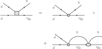
Figure 1: The process $dd\to\eta{}^{4}{\rm He}$ considering explicitly the $\eta^{4}{\rm He}$ re-scattering. The square box in the first diagram indicates the full transition amplitude, while the circle in the second diagram stands for the bare transition amplitude prior to the $\eta^{4}{\rm He}$ final state interaction. It contains all diagrams that do not have $\eta^{4}{\rm He}$ as intermediate state. The oval stands for the $\eta^{4}{\rm He}$ optical potential.

II.1 The $\eta$-${}^{4}\rm{He}$ interaction

The $\eta^{4}\textrm{He}\to\eta^{4}\textrm{He}$ scattering amplitude is given by the diagrams shown in Fig. 2, and formally by the BSE

$$T=V+VGT,$$ (1)

where $G$ is the loop function of intermediate $\eta^{4}{\rm He}$ states, and $V$ is the $\eta^{4}\textrm{He}$ optical potential, which contains an imaginary part to account for the inelastic channels $\eta^{4}\textrm{He}\to X$ with $X$ being mostly $\pi^{3}{\rm He}N$. It also includes the ${}^{3}{\rm He}N^{*}(1535)$ intermediate state arising mainly from the $\eta$ meson absorption, $\eta N\to N^{*}(1535)$ Adlarson:2016dme .

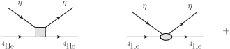
Figure 2: Diagrammatic representation of the $\eta^{4}\textrm{He}\to\eta^{4}{\rm He}$ scattering matrix.

The low density theorem in many-body theory tells us that at low densities the optical potential is given by

$$V(\vec{r})=4t_{\eta N}\tilde{\rho}(\vec{r}),$$ (2)

where $t_{\eta N}$ is the forward $\eta N$ amplitude and $\tilde{\rho}(\vec{r})$ is the ${}^{4}\rm{He}$ density normalized to unity. Eq. (2) is relatively accurate in many body physics, but here we do not use it. We only take from it the density dependence which provides a realistic range of the $\eta$-nucleus interaction, since the $\eta$ can interact with all the nucleons in the nucleus distributed according to $\rho(\vec{r})$.

In momentum space the potential is given by

$$V(\vec{p}_{\eta},\vec{p^{\prime}}_{\eta}) = 4t_{\eta N}\int\mbox{$\textrm{d}$}^{3}\vec{r}\,\tilde{\rho}(\vec{r})e^{i(\vec{p}_{\eta}-\vec{p^{\prime}}_{\eta})\cdot\vec{r}}$$ (3)

$$= 4t_{\eta N}F(\vec{p}_{\eta}-\vec{p^{\prime}}_{\eta}),$$

where $F(\vec{q})$ is the ${}^{4}\rm{He}$ form factor,

$$F(\vec{q})=\int\mbox{$\textrm{d}$}^{3}\vec{r}\,\tilde{\rho}(\vec{r})e^{i\vec{q}\cdot\vec{r}},$$ (4)

and $F(\vec{0})=1$. A good approximation to this form factor at small momentum transfers is given by a Gaussian,

$$F(\vec{q})=e^{-\beta^{2}|\vec{q}|^{2}},$$ (5)

where $\beta^{2}=\langle r^{2}\rangle/6$. This mean-square radius corresponds to the distribution of the centers of the nucleons and, after correcting for the nucleon size, it leads to an experimental value of $\beta^{2}=12.1~{}{\rm GeV}^{-2}$ which was obtained with $\langle r^{2}\rangle^{1/2}_{{}^{4}{\rm He}}=1.68$ fm as in Ref. Sick:2014yha .

Because of this form factor, the optical potential in Eq. (3) contains all partial waves. After integrating over the angle between $\vec{p}^{~{}^{\prime}}_{\eta}$ and $\vec{p}_{\eta}$, the $s$-wave projection of the optical potential becomes

$$V(\vec{p}_{\eta},\vec{p}^{~{}^{\prime}}_{\eta}) \!\!=\!\! 4t_{\eta N}\frac{1}{2}\int^{1}_{-1}\!\!\!\mbox{$\textrm{d}$}\cos\theta e^{-\beta^{2}(|\vec{p}_{\eta}|^{2}+|\vec{p^{\prime}}_{\eta}|^{2}-2|\vec{p}_{\eta}||\vec{p^{\prime}}_{\eta}|\cos\theta)}$$ (6)

$$=4t_{\eta N}e^{-\beta^{2}|\vec{p}_{\eta}|^{2}}e^{-\beta^{2}|\vec{p^{\prime}}_{\eta}|^{2}}\left[1+\frac{1}{6}(2\beta^{2}|\vec{p}_{\eta}||\vec{p^{\prime}}_{\eta}|)^{2}+...\right]\!.$$

One can easily see that the terms $(2\beta^{2}|\vec{p}_{\eta}||\vec{p^{\prime}}_{\eta}|)^{2}/6+...$ are negligible in the region where $e^{-\beta^{2}|\vec{p}_{\eta}|^{2}}e^{-\beta^{2}|\vec{p^{\prime}}_{\eta}|^{2}}$ is sizeable and this leads to a potential that is separable in the variables $\vec{p}_{\eta}$ and $\vec{p}^{~{}^{\prime}}_{\eta}$, which makes the solution of Eq. (1) trivial. Keeping the relativistic factors of the BSE, we can write Oset:1997it :

$$T(\vec{p}_{\eta},\vec{p^{\prime}}_{\eta}) = \tilde{V}e^{-\beta^{2}|\vec{p}_{\eta}|^{2}}e^{-\beta^{2}|\vec{p^{\prime}}_{\eta}|^{2}}+$$

$$\int\frac{\mbox{$\textrm{d}$}^{3}\vec{q}}{(2\pi)^{3}}\frac{M_{{}^{4}{\rm He}}}{2\omega_{\eta}(\vec{q})E_{{}^{4}{\rm He}}(\vec{q})}\frac{\tilde{V}e^{-\beta^{2}|\vec{p}_{\eta}|^{2}}e^{-\beta^{2}|\vec{q}\hskip 1.42262pt|^{2}}}{\sqrt{s}-\omega_{\eta}(\vec{q})-E_{{}^{4}{\rm He}}(\vec{q})+i\epsilon}T(\vec{q},\vec{p^{\prime}}_{\eta}),$$

with $\sqrt{s}$ being the invariant mass of the $\eta^{4}{\rm He}$ system, $\omega_{\eta}(\vec{q})=\sqrt{m^{2}_{\eta}+|\vec{q}\hskip 1.42262pt|^{2}}$, and $E_{{}^{4}{\rm He}}(\vec{q})=\sqrt{M^{2}_{{}^{4}{\rm He}}+|\vec{q}\hskip 1.42262pt|^{2}}$. Note that here we have taken $\tilde{V}$ instead of $4t_{\eta N}$ for more generality.

The $T$ matrix can be factorized in the same way as $V$, and we have Xie:2016zhs

$$T(\vec{p}_{\eta},\vec{p^{\prime}}_{\eta})=te^{-\beta^{2}|\vec{p}_{\eta}|^{2}}e^{-\beta^{2}|\vec{p^{\prime}}_{\eta}|^{2}}.$$ (8)

The BSE becomes then algebraic

$$t=\tilde{V}+\tilde{V}Gt,$$ (9)

with a loop function

$$G(\sqrt{s})=\frac{M_{{}^{4}{\rm He}}}{16\pi^{3}}\times$$

$$\int\frac{\mbox{$\textrm{d}$}^{3}\vec{q}}{\omega_{\eta}(\vec{q})E_{{}^{4}{\rm He}}(\vec{q})}\frac{e^{-2\beta^{2}|\vec{q}|^{2}}}{\sqrt{s}-\omega_{\eta}(\vec{q})-E_{{}^{4}{\rm He}}(\vec{q})+i\epsilon}.$$ (10)

In Fig. 3, we show the real and imaginary parts of the loop function $G$ as a function of the excess energy $Q$ ($Q=\sqrt{s}-m_{\eta}-M_{{}^{4}{\rm He}}$) with $M_{{}^{4}{\rm He}}=3728.4$ MeV and $m_{\eta}=547.862$ MeV. We can see a strong cusp of the real part at the $\eta^{4}{\rm He}$ threshold and the imaginary part starting from this threshold.

Figure 3: Real (solid line) and imaginary (dashed line) parts of the $G$ of Eq. (10) as functions of the excess energy $Q$.

In the normalization that we are using, the $\eta$-nucleon and $\eta$-⁴He scattering lengths are related to the $t$-matrices by

$$a_{\eta N} = \left.\frac{1}{4\pi}\frac{m_{N}}{\sqrt{s_{\eta N}}}t_{\eta N}\right|_{\sqrt{s_{\eta N}}=m_{N}+m_{\eta}}$$ (11)

$$a_{\eta^{4}{\rm He}} = \left.\frac{1}{4\pi}\frac{M_{{}^{4}{\rm He}}}{\sqrt{s}}T\right|_{\sqrt{s}=M_{{}^{4}{\rm He}}+m_{\eta}}.$$ (12)

The strategy that we adopt is to fit $\tilde{V}$ to the $dd\to\eta{}^{4}{\rm He}$ data and then see how different $\tilde{V}$ is from $4t_{\eta N}$ by evaluating

$$a^{\prime}_{\eta N}=\left.\frac{1}{4\pi}\frac{m_{N}}{\sqrt{s_{\eta N}}}\frac{\tilde{V}}{4}\right|_{\sqrt{s_{\eta N}}=m_{N}+m_{\eta}}$$ (13)

and comparing it to the theoretical value of $a_{\eta N}$.

After obtaining the best value for $\tilde{V}$, we then plot

$$T=te^{-2\beta^{2}|\vec{p}_{\eta}|^{2}}$$ (14)

and investigate it below threshold.

II.2 Production amplitude

Following the formalism of Refs. Wronska:2005wk ; Ikeno:2017xyb , we write for the $dd\to\eta{}^{4}{\rm He}$ transition depicted as a circle in Fig. 1

$$V_{P}=A(\vec{\epsilon}_{1}\times\vec{\epsilon}_{2})\cdot\vec{p}_{d},$$ (15)

where $\vec{\epsilon}_{1}$ and $\vec{\epsilon}_{2}$ are the polarizations of the initial two deuterons, and $\vec{p}_{d}$ is the momentum in the initial state. This amplitude has the initial-state $p$-wave needed to match the $\eta(0^{-})^{4}{\rm He}(0^{+})$ with the $d(1^{+})d(1^{+})$ system. This vertex accounts for all mechanisms of $dd\to\eta^{4}{\rm He}$ reaction which do not have $\eta^{4}{\rm He}$ as an intermediate step, as direct $dd\to\eta^{4}{\rm He}$, $dd\to\pi^{3}{\rm He}N\to\eta^{4}{\rm He}$, $dd\to\pi NNNN\to\eta^{4}{\rm He}$, etc.

With similar arguments to those used to derive Eq. (3), we can justify that $V_{P}$ in Eq. (15) must be accompanied by the factor $e^{-\beta^{2}|\vec{p}_{\eta}|^{2}}$, which, if the $\eta$ is in the loop, will become $e^{-\beta^{2}|\vec{q}|^{2}}$. In view of this we can write analytically the equation for the diagrams of Fig. 1 as,

$$t_{dd\to\eta^{4}{\rm He}} = V_{P}e^{-\beta^{2}|\vec{p}_{\eta}|^{2}}+V_{P}Gte^{-\beta^{2}|\vec{p}_{\eta}|^{2}}$$ (16)

$$\!=\! V_{P}e^{-\beta^{2}|\vec{p}_{\eta}|^{2}}(1+Gt)\!=\!\frac{V_{P}e^{-\beta^{2}|\vec{p}_{\eta}|^{2}}}{1-\tilde{V}G},$$

where in the last step we have used Eq. (1). The cross section then becomes

$$\sigma=\frac{M^{2}_{d}M_{{}^{4}{\rm He}}}{9\pi s}\frac{|A|^{2}}{|1-\tilde{V}G|^{2}}|\vec{p}_{\eta}||\vec{p}_{d}|e^{-2\beta^{2}|\vec{p}_{\eta}|^{2}},$$ (17)

where we have used

$$\overline{\sum}\sum|V_{P}|^{2}=\frac{2}{9}|A|^{2}|\vec{p}_{d}|^{2}.$$ (18)

This allows us to perform a fit to the data up to an excess energy $Q=8.5$ MeV, and thus determine $\tilde{V}$. From this we shall determine $T$ by means of Eqs. (8) and (9), and investigate its structure below threshold.

We should note that we are taking both $A$ and $\tilde{V}$ constant. Certainly these magnitudes are energy dependent. The relevant data for the study of the $\eta^{4}{\rm He}\to\eta^{4}{\rm He}$ scattering amplitude are in a range of $2.5$ MeV where changes in these magnitudes should be negligible. The most critical case would be the magnitude $\tilde{V}$, related to $t_{\eta N}$, which is dominated by the $N^{*}(1535)$ pole. To estimate the changes in this magnitude we have used the model of Ref. chiang and looked at the dependence on the energy. We find that the changes in this magnitude in a range of $2.5$ MeV are of the order of $1-2\%$ playing with the uncertainties of the model. This uncertainty is much smaller than the errors that we find from a fit to the data and justify taking $\tilde{V}$ as a constant, and $A$ a fortiori since it is not driven by a resonance.

III Results

We perform a three-parameter [$|A|=r_{A}$ and $\tilde{V}={\rm Re}(V)+i{\rm Im}(V)$] $\chi^{2}$ fit to the experimental data on the total cross sections of the $dd\to\eta{}^{4}{\rm He}$ reaction below $Q=8.5$ MeV. There are 12 experimental data points in total. The values of the resulting parameters are collected in Table 1. One can see that the fitted parameters have large uncertainties, especially for the real part of $\tilde{V}$.

Table 1: Values of parameters determined in this work.

Parameter	Fitted value
$r_{A}[{\rm MeV}^{-5/2}]$	$(7.6\pm 2.3)\times 10^{-9}$
${\rm Re}(V)[{\rm MeV}^{-1}]$	$(-12.3\pm 18.4)\times 10^{-2}$
${\rm Im}(V)[{\rm MeV}^{-1}]$	$(-13.7\pm 5.4)\times 10^{-2}$

To get more precise information from the experimental measurements, we generate random sets of the experimental data within the range of error of each datum with a Gaussian distribution. For each set of data, we perform a $\chi^{2}$ fit, and the corresponding fitted parameters are determined by the best fit. In this way, we get sets of the fitted parameters ($r_{A}$, ${\rm Re}(V)$, ${\rm Im}(V)$) with different best $\chi^{2}_{\rm best}$ Landay:2016cjw ; Perez:2014jsa . With these best fits we get the shaded region  shown in Fig. 4, from where one can see that the experimental data can be well reproduced. Besides, in Fig. 4 we also show the fitted total cross sections with the centroid values of the fitted parameters listed in Table 1 by the red-solid curve. To get values for the observables we evaluate them with the parameters of each fit and from there we get the average value and the dispersion. In this way we take into account the correlations between the parameters.

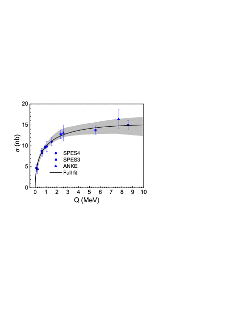
Figure 4: The fitted $dd\to\eta^{4}{\rm He}$ total cross sections compared with experimental data. The circles are taken from Ref. Frascaria:1994va ; squares are from Ref. Willis:1997ix ; and triangles are from Ref. Wronska:2005wk .

On the other hand, as is general in particle physics, and in particular in the case of the $\eta^{4}{\rm He}$ scattering matrix, the position of the poles of $T$ does not coincide with that of the mass and width of a possible Breit-Wigner parametrization. We investigate the position of the poles here. In table 2 we show the position of the poles ($z_{R}=E-i\Gamma/2$) with the energy $E$ measured from the $\eta^{4}{\rm He}$ threshold.

Table 2: Pole position of the $T$ matrix for the $\eta^{4}{\rm He}\to\eta^{4}{\rm He}$ scattering.

${\rm Re}(V)~{}[{\rm MeV}^{-1}]$	${\rm Im}(V)~{}[{\rm MeV}^{-1}]$	$E$ [MeV]	$\Gamma$ [MeV]
$-0.123$	$-0.137$	$10.0$	$13.3$
$-0.2$	$-0.15$	$2.0$	$26.9$
$-0.2$	$-0.1$	$-0.4$	$16.2$
$-0.22$	$-0.1$	$-2.4$	$17.8$
$-0.24$	$-0.1$	$-4.5$	$19.2$
$-0.26$	$-0.1$	$-6.6$	$20.4$
$-0.26$	$-0.08$	$-7.2$	$16.1$
$-0.26$	$-0.06$	$-7.6$	$11.9$
$-0.26$	$-0.04$	$-7.9$	$7.9$
$-0.28$	$-0.1$	$-8.9$	$21.4$

We can see that for the centroid values of $\tilde{V}$ in table 1 we get a pole in the unbound region around $10.6$ MeV and with $\Gamma$ around $11.4$ MeV. Stretching the errors in ${\rm Re}(V)$ in table 1, if we take ${\rm Re}(V)=-0.2$ MeV^-1 and ${\rm Im}(V)=-0.1{\rm MeV}^{-1}$ we find now a pole with $E$ around $-0.4$ MeV and width $\Gamma$ of about $16.2$ MeV. To complete the table we show what happens if we increase ${\rm Re}(V)$ in size in the range of table 1. For ${\rm Re}(V)=-0.24{\rm MeV}^{-1}$ and ${\rm Im}(V)=-0.1{\rm MeV}^{-1}$ we find already a bound state around $E=-4.5$ MeV and with a width $\Gamma$ of about $19.2$ MeV. In conclusion, because of the limited experimental data, we cannot always find a bound state with the fitted potential, which coincides with the conclusion of Ref. Xie:2016zhs for $\eta^{3}{\rm He}$ and the conclusions of Refs. Ikeno:2017xyb ; Skurzok:2018paa .

We also observe the general trend that the widths are bigger than the binding.

In order to understand the results of our analysis more clearly, we plot three areas inside the ${\rm Re}(V)$-${\rm Im}(V)$ plane as shown in Fig. 5, where the acceptable region of ${\rm Re}(V)$ and ${\rm Im}(V)$ values can be easily understood for having an $\eta^{4}{\rm He}$ bound state. The poles in areas I and II are in the unbound and bound regions, respectively, while there is no pole in area III. In Fig. 5, we show also the fitted results of the pairs of ${\rm Re}(V)$ and ${\rm Im}(V)$, which correspond to those best fits as discussed above.

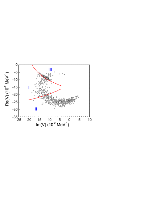
Figure 5: Poles area in the ${\rm Re}(V)$-${\rm Im}(V)$ plane, where the circles are the best fitted pairs of [${\rm Re}(V),{\rm Im}(V)$].

On the other hand, with the potentials $\tilde{V}$ obtained from the best fits as shown in Fig. 5, we have evaluated the scattering length $a^{\prime}_{\eta N}$ of Eq. (13):

$$a^{\prime}_{\eta N}=[-(0.39\pm 0.19)-i(0.23\pm 0.12)]~{}~{}{\rm fm},$$ (19)

which is comparable with the value obtained in Ref. Xie:2016zhs within errors. The errors quoted here are statistical and they are determined as the standard deviation.

Similarly, by means of Eq. (12), we calculate the $\eta^{4}{\rm He}$ scattering length to be

$$a_{\eta^{4}{\rm He}}=[(2.11\pm 1.07)-i(1.21\pm 0.67)]~{}~{}{\rm fm}.$$ (20)

The value of $a_{\eta^{4}{\rm He}}$ obtained here is different from the results obtained in Refs. Willis:1997ix ; Wronska:2005wk ; Ikeno:2017xyb , while the absolute value of $a_{\eta^{4}{\rm He}}$ is compatible with the results of these works.

Note that the strategy of fitting an optical potential to the data instead of the usual $t$-matrix parametrization used in previous works, allows us to determine the sign of the real part of the scattering lengths.

The fit done here produces an attractive potential, which is consistent with all theoretical derivations of $t_{\eta N}$, together with the $t_{\eta N}\tilde{\rho}(\vec{r})$ assumption for the optical potential.

One should also note that in Ref. Xie:2016zhs one not only fitted the $pd\to\eta^{3}{\rm He}$ total cross sections but also the asymmetry parameter in terms of the $\eta$ momentum. Also the quality of the data of $pd\to\eta^{3}{\rm He}$ reaction is much better than for the present reaction. As a consequence, we could determine the parameters in the case of the $\eta^{3}{\rm He}$ interaction with more precision than in the present case.

Since we have less precision than in the $pd\to\eta^{3}{\rm He}$ reaction we investigate what happens by adding more theoretical constraints. For this we assume now that Eq. (2) is changed to

$$V(r^{\prime})=4\bar{t}_{\eta N}\tilde{\rho}(r^{\prime}),$$ (21)

where $\bar{t}_{\eta N}$ is the $\eta N\to\eta N$ scattering amplitude modified in the medium, obtained in Ref. chiang , assuming that the driving term for the $\bar{t}_{\eta N}$ amplitude is given by the excitations of the $N^{*}(1535)$ and changes in the mass of $N^{*}(1535)$ and its width are calculated within many body theory. Then we make random choices of all the variables in the model within their uncertainties. The $\bar{t}_{\eta N}$ amplitude is now given by chiang

$$\bar{t}_{\eta N} = \frac{g^{2}_{\eta}}{\sqrt{s_{\eta N}}-M_{N^{*}}+i\Gamma_{N^{*}}/2-\delta_{M^{*}}+i\delta_{\Gamma_{N^{*}}}/2},$$ (22)

with

$$g^{2}_{\eta} = \frac{2\pi\Gamma_{N^{*}}{\rm Br}(N^{*}\to\eta N)M_{N^{*}}}{m_{N}q_{\eta}},$$ (23)

$$q_{\eta} = \frac{\sqrt{[M^{2}_{N^{*}}-(m_{N}+m_{\eta})^{2}][M^{2}_{N^{*}}-(m_{N}-m_{\eta})^{2}]}}{2M_{N^{*}}},$$ (24)

and we take

$$M_{N^{*}} = 1530\pm 15~{}~{}{\rm MeV},$$ (25)

$$\Gamma_{N^{*}} = 150\pm 25~{}~{}{\rm MeV},$$ (26)

$$\delta_{M_{N^{*}}} = \pm 50~{}~{}{\rm MeV},$$ (27)

$$\delta_{\Gamma_{N^{*}}} = (0-70)~{}~{}{\rm MeV},$$ (28)

$${\rm Br}(N^{*}\to\eta N) = (42.5\pm 12.5)\%.$$ (29)

The results of ${\rm Re(V)}\equiv{\rm Re}(4\bar{t}_{\eta N})$ and ${\rm Im(V)}\equiv{\rm Im}(4\bar{t}_{\eta N})$ are shown in Fig. 6. We see that we get a fair distribution of possible pairs of (${\rm Re}(V)$, ${\rm Im}(V)$) playing with the uncertainties. Yet, the overlap with the distribution of Fig. 5, shows that only part of the solutions with poles in the continuum and the solutions with no poles are acceptable. The bound solutions are far away from the overlap region.

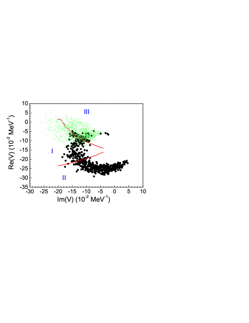
Figure 6: (color online) Poles area in the ${\rm Re}(V)$-${\rm Im}(V)$ plane, where the blacks dots are the best fitted pairs of [${\rm Re}(V),{\rm Im}(V)$] and the green circles are obtained with Eq. (22).

Figure 7: Square of the absolute value of the $\eta^{4}{\rm He}\to\eta^{4}{\rm He}$ scattering amplitude.

We have taken a sample of potentials in the overlap region of Fig. 6 and evaluate $T$ and $|T|^{2}$. The numerical results for the $|T|^{2}$ are shown in Fig. 7. We see that in all cases there is a bump structure below the $\eta^{4}{\rm He}$ threshold, which is tied to the fast increase of the $dd\to\eta^{4}{\rm He}$ cross sections close to the reaction threshold.

In Fig. 8, we show separately the real and imaginary parts of $T$ for these solutions. We see that around $Q=-8$ MeV, ${\rm Re}(T)$ passes through zero, and $|{\rm Im}(T)|$ has a bump around $-4$ MeV. This structure is reminding of a Breit-Wigner form, but somewhat distorted since the position of the maximum of $|{\rm Im}(T)|$ and the zero of ${\rm Re}(T)$ do not coincide.

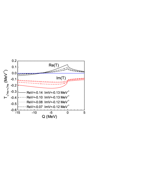
Figure 8: (color online) Real and imaginary parts of the $\eta^{4}{\rm He}\to\eta^{4}{\rm He}$ amplitude $T$ as a function of the excess energy $Q$.

IV Summary and conclusions

We have performed an analysis of the data on the total cross sections of the $dd\to\eta{}^{4}{\rm He}$ reaction close to threshold. Unlike former approaches that make a parametrization of the amplitude, we express the total cross sections in terms of an optical potential from which the $\eta^{4}{\rm He}$ scattering amplitude is evaluated. The $T$ matrix is evaluated from the potential using the Bethe-Salpeter equation and the loop function $G$ of the intermediate $\eta^{4}{\rm He}$ state. This reflects the range of the $\eta^{4}{\rm He}$ interaction, as given by the empirical density of the ${}^{4}{\rm He}$ nucleus.

The potential and other parameters related to the production vertices are fitted to the data and with this potential we search for possible poles of the $\eta^{4}{\rm He}$ system. We found poles in the unbound energy region, in the bound region or no poles at all. We also obtain an $\eta^{4}{\rm He}$ scattering length of the order of $[(2.11\pm 1.07)-i(1.21\pm 0.67)]~{}{\rm fm}$.

In order to put restrictions on the solutions obtained from the $dd\to\eta^{4}{\rm He}$ total cross sections we used a theoretical model for the $\eta^{4}{\rm He}$ scattering amplitude in the nuclear medium based on the excitation of the $N^{*}(1535)$ by $\eta N$ and the medium modifications of this resonance studied in Ref. chiang , playing with all uncertainties in the parameters of the model. In this way we obtained a relatively wide region of values for the $\eta^{4}{\rm He}$ potential, and the overlap with the solutions from the analysis of the data on the $dd\to\eta^{4}{\rm He}$ reaction eliminated many of the solutions allowed by $dd\to\eta^{4}{\rm He}$ alone. Taking the solutions from the overlap region, we could see that in these cases there was a bump structure of $|T|^{2}$ below threshold, closely related to the shape of the $\eta^{4}{\rm He}$ production cross sections close to threshold.

In summary, the new approach to the analysis of the $dd\to\eta{}^{4}{\rm He}$ data close to threshold has proved quite useful and has been able to provide information on $\eta^{4}{\rm He}$ interaction.

It remains to be seen if the structure found below threshold could be seen in some experiments. The broad shape of $|T|^{2}$ in Fig. 7 would not make the matter easy, and in addition one should take into account that large contributions of background source from reactions not tied to the direct $\eta^{4}{\rm He}$ interaction would further blur a possible signal. A message we found from the analysis of $dd\to\eta^{4}{\rm He}$ data is that due to the limited data and the large errors in the fit, we find that these data cannot confirm nor rule out the existence of poles in the bound region, which would correspond to $\eta^{4}{\rm He}$ bound states. In any case, when bound states appear we still see the general rule that the widths are larger than the binding energies.

The last part of our investigation was to combine the $dd\to\eta^{4}{\rm He}$ data with a theoretical model accommodating large uncertainties and from the overlap of the potentials allowed by this model and the data of $dd\to\eta^{4}{\rm He}$ reaction we could see that the solutions leading to bound states were rejected. Yet, for the remaining solutions there was always a broad structure of $|T|^{2}$ below threshold independently that the potentials lead to poles in the continuum or no poles at all.

References

- [1] C. Wilkin, Acta Phys. Polon. B 47, 249 (2016).
- [2] S. D. Bass and P. Moskal, Acta Phys. Polon. B 47, 373 (2016).
- [3] Q. Haider and L. C. Liu, Int. J. Mod. Phys. E 24, 1530009 (2015).
- [4] N. G. Kelkar, Acta Phys. Polon. B 46, 113 (2015).
- [5] S. Hirenzaki, H. Nagahiro, N. Ikeno, and J. Yamagata-Sekihara, Acta Phys. Polon. B 46, 121 (2015).
- [6] E. Friedman, A. Gal, and J. Mare, Phys. Lett. B 725, 334 (2013).
- [7] R. S. Bhalerao and L. C. Liu, Phys. Rev. Lett. 54, 865 (1985).
- [8] Q. Haider and L. C. Liu, Phys. Lett. B 172, 257 (1986).
- [9] L. C. Liu and Q. Haider, Phys. Rev. C 34, 1845 (1986).
- [10] H. C. Chiang, E. Oset, and L. C. Liu, Phys. Rev. C 44, 738 (1991).
- [11] T. Inoue and E. Oset, Nucl. Phys. A 710, 354 (2002).
- [12] C. Garcia-Recio, J. Nieves, T. Inoue, and E. Oset, Phys. Lett. B 550, 47 (2002).
- [13] A. Cieplý, E. Friedman, A. Gal, and J. Mareš, Nucl. Phys. A 925, 126 (2014).
- [14] N. Barnea, E. Friedman, and A. Gal, Phys. Lett. B 747, 345 (2015).
- [15] N. Barnea, E. Friedman and A. Gal, Nucl. Phys. A 968, 35 (2017).
- [16] J. J. Xie, W. H. Liang, E. Oset, P. Moskal, M. Skurzok and C. Wilkin, Phys. Rev. C 95, 015202 (2017).
- [17] R. Bilger et al., Phys. Rev. C 65, 044608 (2002).
- [18] T. Mersmann et al., Phys. Rev. Lett. 98, 242301 (2007).
- [19] C. Wilkin et al., Phys. Lett. B 654, 92 (2007).
- [20] J. Urban et al. [COSY-GEM Collaboration], Int. J. Mod. Phys. A 24, 206 (2009).
- [21] R. Frascaria et al., Phys. Rev. C 50, R537 (1994).
- [22] N. Willis et al., Phys. Lett. B 406, 14 (1997).
- [23] A. Wronska et al., Eur. Phys. J. A 26, 421 (2005).
- [24] M. Skurzok, P. Moskal and W. Krzemien, Prog. Part. Nucl. Phys. 67, 445 (2012).
- [25] P. Adlarson et al. [WASA-at-COSY Collaboration], Phys. Rev. C 87, 035204 (2013).
- [26] W. Krzemie et al. [WASA-at-COSY Collaboration], Acta Phys. Polon. B 45, 689 (2014).
- [27] W. Krzemie et al. [WASA-COSY Collaboration], Acta Phys. Polon. B 46, 757 (2015).
- [28] M. Skurzok et al. [WASA-at-COSY Collaboration], Acta Phys. Polon. B 47, 503 (2016).
- [29] P. Adlarson et al., Nucl. Phys. A 959, 102 (2017).
- [30] R. E. Chrien et al., Phys. Rev. Lett. 60, 2595 (1988).
- [31] J. D. Johnson et al., Phys. Rev. C 47, 2571 (1993).
- [32] G. A. Sokol, T. A. Aibergenov, A. V. Kravtsov, A. I. L’vov, and L. N. Pavlyuchenko, Fizika B 8, 85 (1999).
- [33] A. Budzanowski et al. [COSY-GEM Collaboration], Phys. Rev. C 79, 012201 (2009).
- [34] P. Moskal and J. Smyrski, Acta Phys. Polon. B 41, 2281 (2010).
- [35] F. Pheron et al., Phys. Lett. B 709, 21 (2012).
- [36] H. Fujioka et al. [Super-FRS Collaboration], Acta Phys. Polon. B 46, 127 (2015).
- [37] T. Rausmann et al., Phys. Rev. C 80, 017001 (2009).
- [38] N. Ikeno, H. Nagahiro, D. Jido and S. Hirenzaki, Eur. Phys. J. A 53, 194 (2017).
- [39] M. Skurzok, P. Moskal, N. G. Kelkar, S. Hirenzaki, H. Nagahiro and N. Ikeno, Phys. Lett. B 782, 6 (2018).
- [40] I. Sick, Phys. Rev. C 90, 064002 (2014).
- [41] E. Oset and A. Ramos, Nucl. Phys. A 635, 99 (1998).
- [42] J. Landay, M. Döring, C. Fernández-Ramírez, B. Hu and R. Molina, Phys. Rev. C 95, 015203 (2017).
- [43] R. Navarro Pérez, J. E. Amaro and E. Ruiz Arriola, Phys. Lett. B 738, 155 (2014).