Convection-Diffusion-Reaction equation with similarity solutions

Abstract

We consider similarity solutions of the generalized convection-diffusion-reaction equation with both space- and time-dependent convection, diffusion and reaction terms. By introducing the similarity variable, the reaction-diffusion equation is reduced to an ordinary differential equation. Matching the resulting ordinary differential equation with known exactly solvable equations, one can obtain corresponding exactly solvable convection-diffusion-reaction systems. Some representative examples of exactly solvable systems are presented. We also describe how an equivalent convection-diffusion-reaction system can be constructed which admits the same similarity solution of another convection-diffusion-reaction system.

I Introduction

The Convection-Diffusion-Reaction (CDR) equation is a class of second order differential that is widely employed to model phenomena that involve the change of concentration/population of one or more substances/species distributed in space under the influence of three processes: local reaction which modify the concentration/population, diffusion which causes the substances/species to spread in space, and convection/drifting under the influence of external forces GK1 ; GK2 ; HM ; CP . This includes as special cases the Fokker-Planck equation [5-13] and the reaction-diffusion equation [14-25]. The CDR equation has found many important applications in physics, chemistry, astrophysics, engineering, and biology.

In view of its broad applicability, it is thus desirable to obtain analytic solutions of the CDR equation for as many systems as possible. However, just as any equation in sciences, solving the CDR equation exactly is in general a formidable task, except in a few simplified cases. Interestingly, many analytic solutions were found in the form of travelling wave solutions GK1 ; GK2 ; HM ; CP .

Different forms of analytic solutions may be possible for the CDR equation. In our previous work, we have studied exact solvability of the Fokker-Planck Ho1 ; Ho2 ; Ho3 and reaction-diffusion equations HL in terms of similarity solutions. Here we would like to extend our previous consideration to the CDR equation.

One advantage of the similarity method is that it allows one to reduce the partial differential equation under consideration to an ordinary differential equation which is generally easier to solve, provided that the original equation possesses proper scaling property under certain scaling transformation of the basic variables.

We shall first discuss the scaling properties of the CDR equation. This includes the scaling forms of the relevant function, and the corresponding similarity variable. The equation of continuity is then considered, which is used to identify two types of scaling behaviours of the CDR equation, namely, systems in which particle number is conserved or not. Some examples of these two types of scaling CDR systems are presented. Finally, we briefly discuss how an equivalent CDR system can be constructed which admits the same similarity solution of another CDR system.

II Scaling form of CDR equation and similarity variable

The $(1+1)$-dimension CDR equation to be studied in this paper is taken to have the following general form

$$\frac{\partial W(x,t)}{\partial t}=\frac{\partial}{\partial x}\left(D(W,x,t)\frac{\partial}{\partial x}W(x,t)\right)$$

$$~{}~{}~{}~{}-\frac{\partial}{\partial x}\left(C(W,x,t)\ W(x,t)\right)+R(W,x,t),$$ (1)

where $W(x,t)$ is the particle number function, $D(W,x,t),C(W,x,t)$ and $R(W,x,t)$ are the diffusion, the convection, and the reaction term, respectively. We use the term “particle” to denote generally the number of basic member of a substance or a specie. The domains we shall consider in this paper are the real line $x\in(-\infty,\infty)$, or the half lines $x\in[0,\infty)$. Cases with finite domains, which correspond to systems with moving boundaries, can be considered similarly Ho2 . We leave the possibility that $C,D$ and $R$ could be functions of $W$ (when no confusion arises, we shall often omit the independent variables of a function for simplicity and clarity of presentation).

If the CDR possesses scaling symmetry, then similarity solution is possible. Suppose under the scale transformation

$$x=\epsilon^{a}\,\bar{x}\;\;\;,\;\;\;t=\epsilon^{b}\,\bar{t},$$ (2)

all the relevant functions of the CDR equation scale as

$$W(x,t)=\epsilon^{\omega}\bar{W}(\bar{x},\bar{t}),~{}~{}C(W,x,t)=\epsilon^{c}\bar{C}(\bar{W},\bar{x},\bar{t});\;\;$$ (3)

$$D(W,x,t)=\epsilon^{d}\bar{D}(\bar{W},\bar{x},\bar{t}),\;\;R(W,x,t)=\epsilon^{r}\bar{R}(\bar{W},\bar{x},\bar{t}).$$

Here the scale factor $\epsilon$ and the scaling exponents $a,b,c,d,r$ and $\omega$ are real parameters.

CDR equation possesses scaling symmetry under the above transformation if the form of the CDR equation expressed in terms of the transformed quantities is the same as the form of the original equation. This is the case if the exponents are related by $b=2a-d=a-c=\omega-r$.

Under this situation, one can transform the second order CDR equation into an ordinary differential equation by introducing the similarity variable $z$, which can be defined as

$$z\equiv\frac{x}{t^{\alpha}},~{}~{}\mbox{where}~{}\alpha=\frac{a}{b}\;\;\;,\;b\neq 0\;.$$ (4)

Suppose the functions $C,D,R$ and $W$ have the following scaling forms:

$$W(x,t) = t^{\mu}y(z),~{}~{}C(W,x,t)=t^{\gamma}\tau(z),$$

$$~{}~{}D(W,x,t) = t^{\delta}\sigma(z),~{}~{}R(W,x,t)=t^{\rho}\rho(z).$$ (5)

From Eq. (3) together with the scaling conditions $b=2a-d=a-c=\omega-r$, one has

$$\mu=\frac{\omega}{b},~{}~{}\gamma=\frac{c}{b}=\alpha-1,~{}~{}\delta=\frac{d}{b}=2\alpha-1,~{}~{}\rho=\frac{r}{b}=\mu-1.$$ (6)

Thus $\alpha$ and $\mu$ are the only two independent scaling exponents of the CDR equation.

In terms of these scaling forms, Eq. (1) reduces to an ordinary differential equation

$$\frac{d}{dz}\left(\sigma\frac{d}{dz}y\right)+\alpha z\frac{dy}{dz}-\frac{d}{dz}\left(\tau y\right)-\mu y+\rho(z)=0,$$ (7)

or equivalently,

$$\sigma y^{\prime\prime}+(\sigma^{\prime}+\alpha\,z-\tau)\,y^{\prime}-(\tau^{\prime}+\mu)\,y+\rho=0.$$ (8)

Here “prime” represents derivative with respect to $z$. Note that when $\mu=-\alpha$, which we will encounter below, Eq. (7) reduces to

$$\frac{d}{dz}\left(\sigma\frac{d}{dz}y+\left(\alpha z-\tau\right)y\right)+\rho(z)=0.$$ (9)

Next we shall consider the condition imposed by the continuity in the change of the particle number of the system, i.e., the equation of continuity.

III Equation of continuity

The total number $N$ of the system is related to the density function $W(x,t)$ by

$$N=\int_{\cal D}\,W(x,t)\,dx=t^{\alpha+\mu}\int_{\cal D}\,y(z)\,dz,$$ (10)

where $\cal D$ is the domain of the independent variable. For simplicity, we use the same notation $\cal{D}$ for both the variable $x$, and the corresponding similarity variable $z$.

Eq. (10) distinguishes two different situations: $\alpha+\mu\neq 0$ and $\alpha+\mu=0$. It is obvious from this equation that $N$ is conserved if and only if $\mu=-\alpha$.

Eq. (10) implies that

$$\frac{dN}{dt}=(\alpha+\mu)t^{\alpha+\mu-1}\left(\int_{\cal D}\,y(z)\,dz\right).$$ (11)

On the other hand, from Eq. (1) one has

$$\frac{dN}{dt}=t^{\alpha+\mu-1}\Delta\left(\sigma\frac{dy}{dz}-\tau y\right)_{\partial{\cal D}}+t^{\alpha+\rho}\int_{\cal D}\rho(z)\,dz.$$ (12)

Here $\partial{\cal D}$ denotes the boundaries of the domain $\cal D$, and $\Delta(\cdots)_{\partial{\cal D}}$ the difference of the terms in the bracket at the boundaries.

In view of $\rho=\mu-1$, one has

$$(\alpha+\mu)\int_{\cal D}\,y(z)\,dz=\int_{\cal D}\,\rho(z)\,dz+\Delta\left(\sigma\frac{dy}{dz}-\tau y\right)_{\partial{\cal D}}.$$ (13)

It is interesting to note that, by integrating Eq. (7) and replacing the integral of $\rho(z)$ in Eq. (13), the equation of continuity simplifies to

$$\Delta(\alpha zy)=0.$$ (14)

Below we discuss separately the cases for $\mu=-\alpha$ and $\mu\neq-\alpha$.

IV Cases with $\mu=-\alpha$

In this case $y(z)$ satisfies eq. (9). As $N$ is conserved when $\mu=-\alpha$, one can normalize $W(x,t)=t^{-\alpha}y(z)$ and treat it as the probability distribution function. Thus the number of particle is

$$N=\int_{\cal D}\,y(z)\,dz,$$ (15)

and the equation of continuity (13) becomes

$$\int_{\cal D}\,\rho(z)\,dz+\Delta\left(\sigma\frac{dy}{dz}-\tau y\right)_{\partial{\cal D}}=0.$$ (16)

Any choice of the set of functions $\sigma(z),\rho(z)$ and $\tau(z))$ such that $y(z)$ is normalizable and Eq.(16) is satisfied defines an exactly solvable CDR system with similarity solution. Formally the solution $y(z)$ is

$$y(z) = -e^{-\int^{z}\,dz\,\frac{\alpha z-\tau}{\sigma}}$$

$$~{}~{}~{}\times\left(\int^{z}\,dze^{\int^{z}\frac{\alpha z-\tau}{\sigma}dz}\frac{1}{\sigma}\,\int^{z}\,dz\,\rho(z)+C\right),$$

where $C$ is an integration constant.

For $y(z),\sigma(z)$ and $\tau(z)$ such that $\Delta(\sigma\,y^{\prime}-\tau y)_{\partial{\cal D}}=0$, one has $\int_{\cal D}\,\rho(z)dz=0$. This is most easily satisfied if $\rho(z)$ is a total differential, i.e., $\rho(z)=-d{\bar{\rho}}(z)/dz$ for some function $\bar{\rho}(z)$ which vanishes at the boundaries, or any function $\rho(z)$ that is anti-symmetric w.r.t. the mid-point of the domain $\cal{D}$ in the similarity variable $z$. This latter situation is possible only if $\cal{D}$ is the whole line or a finite domains in the $z$-space (corresponding to moving boundaries in the $x$-space), and is not possible for the half-line.

If $\rho(z)$ is anti-symmetric w.r.t. the midpoint of $\cal D$, the Eq. (9) implies that $\sigma(z)$ is symmetric, while $\tau(z)$ and $y(z)$ are anti-symmetric. But an anti-symmetric $y(x)$ gives $N=0$ from Eq. (15). Thus this case is not of interest.

So we take $\rho(z)$ to be a total differential. This implies that Eq. (9) is a total derivative, and can be integrated once to give

$$\sigma y^{\prime}+\left(\alpha z-\tau\right)y-{\bar{\rho}}={\rm constant}.$$ (18)

If the functions on the l.h.s. of Eq. (18) vanish at the boundaries, the constant equals zero and we need only to consider the following equation instead

$$\sigma y^{\prime}+\left(\alpha z-\tau\right)y-{\bar{\rho}}=0.$$ (19)

There are two situations that one can consider : Fokker-Planck type and non-Fokker-Planck type. To construct exactly solvable CDR systems, one can follow exactly the procedure presented in HL . So we shall give only the main ideas here.

$\bullet$ Fokker-Planck type

Let the function ${\bar{\rho}}(z)$ be proportional to $y(z)$, i.e. ${\bar{\rho}}(z)=\beta(z)y(z)$ for some function $\beta(z)$. In this case the CDR is of the Fokker-Planck type, where the function $\beta(z)+\tau(z)$ plays the role of the drift coefficient. Integrating Eq. (19) once gives

$$y(z)\propto\exp\left(\int^{z}\,dz\,\frac{\beta(z)+\tau(z)-\alpha z}{\sigma(z)}\right).$$ (20)

Hence for any choice of $\sigma(z),\beta(z)$ and $\tau(z)$ are such that $y(z)$ in Eq. (20) is integrable and normalizable, one has an exactly solvable CDR system. This is exactly the same as the way to obtain similarity solutions of the Fokker-Planck equations discussed in Ho1 ; Ho2 ; Ho3 . All the cases presented there for the Fokker-Planck equations can be carried over to this type of CDR equations. This includes cases related to solutions with moving boundaries, and solutions involving the recently discovered exceptional orthogonal polynomials, can be found in Ref. Ho2 and Ho3 , respectively.

$\bullet$ Non-Fokker-Planck type

For ${\bar{\rho}}(z)$ not proportional to $y(z)$, i.e., ${\bar{\rho}}(z)\neq\beta(z)y(z)$, the general solution of Eq. (IV) is

$$y(z)=e^{-\int^{z}\frac{\alpha z-\tau}{\sigma}dz}\left(\int^{z}e^{\int^{z}\frac{\alpha z-\tau}{\sigma}dz}\frac{\bar{\rho}}{\sigma}dz+C\right),$$ (21)

where $C$ is a constant of integration. Any choice of $\sigma(z),\tau(z)$ and $\bar{\rho}(z)$ such that $y(z)$ is exactly integrable and $W(x,t)$ is nomalizable furnishes a solvable RD system.

Again, the procedures presented in HL can be carried over to construct exactly solvable CDR systems of this type.

V Cases with $\mu\neq-\alpha$

When $\mu\neq-\alpha$, the number of particles does not conserve.

Formally one can construct a solvable CDR system as follows. Defining $\tilde{\rho}(z)\equiv(\tau^{\prime}+\mu)y(z)-\rho(z)$, we rewrite Eq. (8) as

$$y^{\prime\prime}+\frac{\sigma^{\prime}+\alpha\,z-\tau}{\sigma}y^{\prime}=\frac{\tilde{\rho}}{\sigma}.$$ (22)

By first treating this equation as a first order differential equation for $y^{\prime}$ and using the method of integrating factor, one obtains the formal solution of Eq. (22) as

$$y(z) = \int^{z}\,dz^{\prime}\,e^{-\gamma(z^{\prime})}\left[\int^{z^{\prime}}\,dz^{\prime\prime}\,e^{\gamma(z^{\prime\prime})}\frac{\tilde{\rho}(z^{\prime\prime})}{\sigma(z^{\prime\prime})}+C^{\prime}\right]+C,$$ (23)

$$~{}~{}~{}\gamma(z)\equiv\int^{z}\,dz\,\frac{\sigma^{\prime}(z)+\alpha\,z-\tau(z)}{\sigma(z)},$$

where $C$ and $C^{\prime}$ are integrating constants. One then looks for the functions $\sigma(z)$ and $\tilde{\rho}(z)$ that make Eq. (23) integrable. An exactly solvable CDR system is then given by the functions $\sigma(z)$, $y(z)$ and $\rho(z)=(\tau^{\prime}(z)+\mu)y(z)-\tilde{\rho}(z)$.

Of course, while the above recipe gives a formal way to find exactly solvable CDR systems, it is in general not easy to determine the required functions $\sigma(z)$ and $\tilde{\rho}(z)$. A more practical way to look for exactly solvable CDR systems is to match Eq. (22) with the known exactly solvable 2nd-order differential equations. In what follows we shall present some examples based on this latter method.

$\bullet$ Example 1 : $\sigma=1,\tau=\alpha z$

Taking $\sigma=1,\tau=\alpha z$, Eq. (8) becomes

$$y^{\prime\prime}-(\alpha+\mu)\,y+\rho=0,~{}~{}z\in(-\infty,\infty).$$

By matching this equation with the differential equation in $\S 2.1.2.3$ of PZ ,

$$y^{\prime\prime}-(c^{2}z^{2}-c)\,y=0,~{}~{}c>0,$$

which admits a particular solution

$$y_{0}=e^{-\frac{1}{2}cz^{2}},$$ (24)

we get

$$\rho=\left(-c^{2}z^{2}+c+\alpha+\mu\right)\,y.$$

we get a CDR system as follows:

$$C(x,t) = \alpha\,\frac{x}{t},$$

$$D(x,t) = t^{2\alpha-1},~{}~{}y(z)=e^{-\frac{1}{2}cz^{2}},~{}~{}x\in(-\infty,\infty),~{}$$

$$R(x,t) = t^{\mu-1}\left[-c^{2}\left(\frac{x}{t^{\alpha}}\right)^{2}+c+\alpha+\mu\right]e^{-\frac{1}{2}c\left(\frac{x}{t^{\alpha}}\right)^{2}},$$

$$W(x,t) = t^{\mu}e^{-\frac{1}{2}c\left(\frac{x}{t^{\alpha}}\right)^{2}}.$$

$\bullet$ Example 2 : $\sigma=\beta z$

If we match Eq. (8) with the equation in $\S 2.1.2.69$ of PZ ,

$$zy^{\prime\prime}+azy^{\prime}+ay=0,~{}~{}~{}a>0,~{}z\in[0,\infty),$$

which has a particular solution

$$y_{0}=z\,e^{-az},$$

then we get a CDR system

$$C(x,t) = t^{\alpha-1}\left((\alpha-\beta a)\,\frac{x}{t^{\alpha}}+\beta\right),$$

$$D(x,t) = \beta\,t^{\alpha-1}\,x,,~{}$$

$$R(x,t) = (\alpha+\mu)\,x\,t^{\mu-\alpha-1}\,e^{-a\frac{x}{t^{\alpha}}},$$

$$W(x,t) = x\,t^{\mu-\alpha}\,e^{-a\frac{x}{t^{\alpha}}}.$$

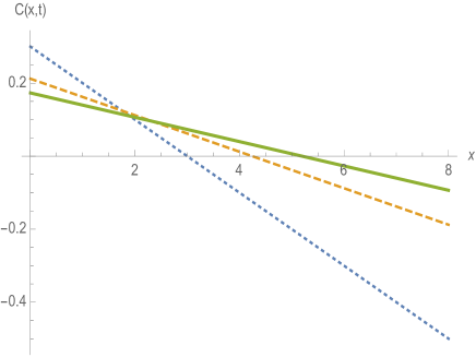
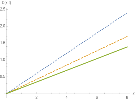
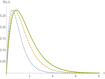
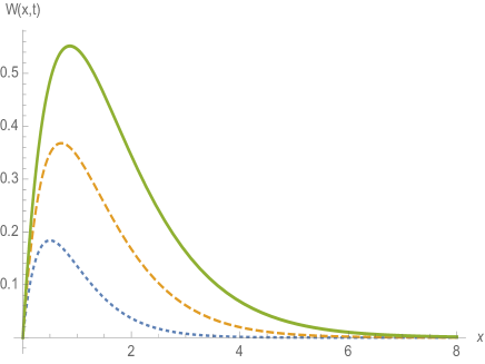
Figure 1: Plot of $C(x,t),D(x,t),R(x,t)$ and $W(x,t)$ for Example 2 with $\alpha=0.5,\beta=0.3,\mu=1,a=2$, and time $t=1$ (dotted), $t=2$ (dashed), $t=3$ (solid).

In Fig. 1 we present the plots of these functions for a set of parameters with three different times.

$\bullet$ Example 3 : $\sigma(z)=-\frac{1}{2}(\alpha+\mu)z^{2}$

With

$$\sigma(z) = -\frac{1}{2}(\alpha+\mu)z^{2},~{}~{}~{}\tau(z)=-\mu z,$$

$$\rho(z) = \frac{1}{2}(\alpha+\mu)z^{2}\left(g^{2}(z)+g^{\prime}(z)\right]\,y(z),$$ (25)

where $g(z)$ is some function of $z$, Eq. (8) becomes

$$y^{\prime\prime}-(g^{2}+g^{\prime})y=0.$$ (26)

This equation admits a particular solution

$$y_{0}(z)=e^{\int^{z}g(z)dz}.$$ (27)

One can choose $g(z)$ such that $y(z)\to 0$ fast enough so that the boundary terms go to zero. This give us an exactly solvable CDR system with

$$C(x,t) = -\mu\,\frac{x}{t};$$

$$D(x,t) = -\frac{1}{2}(\alpha+\mu)\,\frac{x^{2}}{t},$$ (28)

$$R(x,t) = \frac{1}{2}(\alpha+\mu)z^{2}\left(g^{2}(z)+g^{\prime}(z)\right]\exp\left(\int^{z}g(z)dz\right),$$

$$W(x,t) = t^{\mu}\exp\left(\int^{z}g(z)dz\right).$$

VI Nonlinear cases

One can obtain nonlinear CDR systems by matching Eq. (8) with some nonlinear ODEs. We will only illustrate this by a simple example.

$\bullet$ Example 4

The simple nonlinear ODE

$$y^{\prime\prime}-\lambda y^{3}=0,~{}~{}~{}\lambda>0,~{}~{}z\in[0,\infty)$$ (29)

has solution

$$y=\left[\sqrt{\frac{\lambda}{2}}\,z+C\right]^{-1},~{}~{}~{}~{}~{}C>0.$$

We can match Eq. (8) with (29) with, say $\sigma=1$ and $\tau=$constant. This leads to

$$\rho(z)=\mu y+(\alpha z-\tau)\sqrt{\frac{\lambda}{2}}\,y^{2}-\lambda\,y^{3}.$$ (30)

Equation of continuity (13), or (14), requires that $\alpha=0$, and thus $\delta=\gamma=-1$. The corresponding nonlinear CDR system is defined by

$$C(x,t) = \frac{\tau}{t};$$

$$D(x,t) = t^{-1},$$ (31)

$$R(x,t) = t^{\mu-1}\,\left[\mu y-\tau\sqrt{\frac{\lambda}{2}}\,y^{2}-\lambda y^{3}\right],$$

with solution

$$W(x,t)=t^{\mu}\left[\sqrt{\frac{\lambda}{2}}\,x+C\right]^{-1},~{}~{}~{}~{}~{}C>0.$$ (32)

We show in Fig. 2 the graphs of $R(x,t)$ and $W(x,t)$ for a set of parameters with three different times. The functions $C(x,t)$ and $D(x,t)$ are just horizontal lines for fixed time $t$.

VII Equivalent systems

It is noted that solutions $W(x,t)$ of some CDR systems are the same as the solutions of some of the Reaction-Diffusion systems given in HL , with the same exponents $\alpha$ and $\mu$. For instance, the solution of Example 1 in this work is the same as that in Section 6.1 of HL . This prompted us to consider the relation between different CDR systems having the same solution $W(x,t)$ (thus with the same exponents $\alpha$ and $\mu$), but with different diffusion, convention, and reaction terms. We shall call these systems “equivalent systems”.

Consider the following two CDR systems

$$\sigma y^{\prime\prime}+(\sigma^{\prime}+\alpha\,z-\tau)\,y^{\prime}-(\tau^{\prime}+\mu)\,y+\rho=0,$$

$$\tilde{\sigma}y^{\prime\prime}+(\tilde{\sigma}^{\prime}+\alpha\,z-\tilde{\tau})\,y^{\prime}-(\tilde{\tau}^{\prime}+\mu)\,y+\tilde{\rho}=0.$$ (33)

Let these two equations admit the the same solution $y(z)$, then one has

$$\frac{d}{dz}\left[(\tilde{\sigma}-\sigma)y^{\prime}\right]-\frac{d}{dz}\left[(\tilde{\tau}-\tau)y\right]+\left(\tilde{\rho}-\rho\right)=0.$$ (34)

Now suppose we are given the solution of the CDR system given by $\{\sigma,\tau,\rho\}$, which includes the Fokker-Planck and reaction-diffusion equations as special cases, and we want to construct an equivalent system $\{\tilde{\sigma},\tilde{\tau},\tilde{\rho}\}$. This can be done by specifying two of three functions of $\{\tilde{\sigma},\tilde{\tau},\tilde{\rho}\}$, and determine the third one from Eq. (34). An exactly solvable new CDR system is then obtained, provided that Eq. (34) can be exactly solved.

This construction respects the the equation of continuity (13), since Eq. (34) implies the identity

$$\int_{\cal D}\,\rho(z)\,dz+\Delta\left(\sigma\frac{dy}{dz}-\tau y\right)_{\partial{\cal D}}$$

$$= \int_{\cal D}\,\tilde{\rho}(z)\,dz+\Delta\left(\tilde{\sigma}\frac{dy}{dz}-\tilde{\tau}y\right)_{\partial{\cal D}}.$$ (35)

Suppose $\tilde{\sigma}=\sigma$ and $\tilde{\tau}$ are given, then the corresponding $\tilde{\rho}$ of an equivalent CDR will determined by

$$\rho+\frac{d}{dz}\left[(\tilde{\tau}-\tau)y\right].$$ (36)

$\bullet$ Example 5

Example 6.1 of HL is a reaction-diffusion equation defined by (in the notations of this work)

$$\sigma=1,~{}~{}\tau=0,~{}~{}y_{0}=e^{-\frac{1}{2}cz^{2}}$$

$$\rho=[c(\alpha-c)z^{2}+(\mu+c)]y_{0}.$$ (37)

If one wants to construct an equivalent CDR system, say with $\tilde{\sigma}=\sigma=1,\tilde{\tau}=\beta z$ for some constant $\beta$, then the $\tilde{\rho}$ is $\tilde{\rho}=[c(\alpha-\beta-c)z^{2}+(\mu+\beta+c)]y_{0}$. Thus we have infinitely many equivalent CDR systems as $\beta$ is arbitrary. Example  1 given in this work corresponds to the case with $\beta=\alpha$.

If one chooses $\tilde{\sigma}=1$ and $\tilde{\tau}=\beta$, then $\tilde{\rho}=[c(\alpha-c)z^{2}-\beta cz+(\mu+c)]y_{0}$. This can be obtained by Eq. (36) from the systems with $\tau=0$ and $\tau=\beta z$.

$\bullet$ Example 6

We construct a reaction-diffusion equation which is equivalent to the nonlinear CDR system in Example 4 (note that there $\alpha=0$ to satisfies the equation of continuity) .

Setting $\tilde{\sigma}=1$ and $\tilde{\tau}=0$, the required $\tilde{\rho}$ is $\tilde{\rho}=\mu\,y-\lambda\,y^{3}$.

VIII Summary

We have considered solvability of the convection-diffusion-reaction equation with both space- and time-dependent convection, diffusion and reaction terms by means of the similarity method. There are two types of scaling behaviours of the CDR equation, relating to whether particle number is conserved or not. By introducing the similarity variable, the convection-diffusion-reaction equation is reduced to an ordinary differential equation. The reduced ordinary differential equations, namely, Eqs. (8) and (19), are quite simple in their functional forms. Particularly, Eq. (19), which corresponds to the particle conserving cases, is integrable and its solution can be given in closed form. By matching these two ordinary differential equations with some known exactly solvable equations, one can obtain corresponding exactly solvable CDR systems. Some representative examples of exactly solvable systems were presented. Finally, we have briefly discussed how an equivalent CDR system can be constructed which admits the same similarity solution of another CDR system.

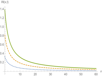
Figure 2: Plot of $R(x,t)$ and $W(x,t)$ for Example 4 with $\alpha=0,\mu=1.3,\lambda=2,\tau=2.4,C=3$ and time $t=1$ (dotted), $t=2$ (dashed), $t=3$ (solid).