High Dimensional Robust Sparse Regression

Abstract

We provide a novel – and to the best of our knowledge, the first – algorithm for high dimensional sparse regression with constant fraction of corruptions in explanatory and/or response variables. Our algorithm recovers the true sparse parameters with sub-linear sample complexity, in the presence of a constant fraction of arbitrary corruptions. Our main contribution is a robust variant of Iterative Hard Thresholding. Using this, we provide accurate estimators: when the covariance matrix in sparse regression is identity, our error guarantee is near information-theoretically optimal. We then deal with robust sparse regression with unknown structured covariance matrix. We propose a filtering algorithm which consists of a novel randomized outlier removal technique for robust sparse mean estimation that may be of interest in its own right: the filtering algorithm is flexible enough to deal with unknown covariance. Also, it is orderwise more efficient computationally than the ellipsoid algorithm. Using sub-linear sample complexity, our algorithm achieves the best known (and first) error guarantee. We demonstrate the effectiveness on large-scale sparse regression problems with arbitrary corruptions.

1 Introduction

Learning in the presence of arbitrarily (even adversarially) corrupted outliers in the training data has a long history in Robust Statistics [27, 23, 42], and has recently received much renewed attention. The high dimensional setting poses particular challenges as outlier removal via preprocessing is essentially impossible when the number of variables scales with the number of samples. We propose a computationally efficient estimator for outlier-robust sparse regression that has near-optimal sample complexity, and is the first algorithm resilient to a constant fraction of arbitrary outliers with corrupted covariates and/or response variables. Unless we specifically mention otherwise, all future mentions of outliers mean corruptions in covariates and/or response variables.

We assume that the authentic samples are independent and identically distributed (i.i.d.) drawn from an uncorrupted distribution $P$, where $P$ represents the linear model $y_{i}=\bm{x}_{i}^{\top}\bm{\beta}^{*}+\xi_{i}$, where $\bm{x}_{i}\sim\mathcal{N}\left(0,\bm{\Sigma}\right)$, and $\bm{\beta}^{*}\in\operatorname{\mathbb{R}}^{d}$ is the true parameter (see Section 1.3 for complete details and definitions). To model the corruptions, the adversary can choose an arbitrary $\epsilon$-fraction of the authentic samples, and replace them with arbitrary values. We refer to the observations after corruption as $\epsilon$-corrupted samples (Definition 1.1). This corruption model allows the adversary to select an $\epsilon$-fraction of authentic samples to delete and corrupt, hence it is stronger than Huber’s $\epsilon$-contamination model [26], where the adversary independently corrupts each sample with probability $\epsilon$.

Outlier-robust regression is a classical problem within robust statistics (e.g., [39]), yet even in the low-dimensional setting, efficient algorithms robust to corruption in the covariates have proved elusive, until recent breakthroughs in [38, 15] and [31], which built on important results in Robust Mean Estimation [13, 33] and Sums of Squares [4], respectively.

In the sparse setting, the parameter $\beta^{\ast}$ we seek to recover is also $k$-sparse, and a key goal is to provide recovery guarantees with sample complexity scaling with $k$, and sublinearly with $d$. Without outliers, by now classical results (e.g., [18]) show that $n=\Omega(k\log d)$ samples from a i.i.d sub-Gaussian distribution are enough to give recovery guarantees on $\beta^{\ast}$ with and without additive noise. These strong assumptions on the probabilistic distribution are necessary, since in the worst case, sparse recovery is known to be NP-hard [3, 48].

Sparsity recovery with a constant fraction of arbitrary corruption is fundamentally hard. For instance, to the best of our knowledge, there’s no previous work can provide exact recovery for sparse linear equations with arbitrary corruption in polynomial time. In contrast, a simple exhaustive search can easily enumerate the samples and recover the sparse parameter in exponential time.

In this work, we seek to give an efficient, sample-complexity optimal algorithm that recovers $\beta^{\ast}$ to within accuracy depending on $\epsilon$ (the fraction of outliers). In the case of no additive noise, we are interested in algorithms that can guarantee exact recovery, independent of $\epsilon$.

1.1 Related work

The last 10 years have seen a resurgence in interest in robust statistics, including the problem of resilience to outliers in the data. Important problems attacked have included PCA [32, 47, 46, 33, 13], and more recently robust regression (as in this paper) [38, 15, 17, 31] and robust mean estimation [13, 33, 1], among others. We focus now on the recent work most related to the present paper.

Robust regression. Earlier work in robust regression considers corruption only in the output, and shows that algorithms nearly as efficient as for regression without outliers succeeds in parameter recovery, even with a constant fraction of outliers [34, 37, 5, 6, 30]. Yet these algorithms (and their analysis) focus on corruption in $y$, and do not seem to extend to the setting of corrupted covariates – the setting of this work. In the low dimensional setting, there has been remarkable recent progress. The work in [31] shows that the Sum of Squares (SOS) based semidefinite hierarchy can be used for solving robust regression. Essentially concurrent to the SOS work, [12, 24, 38, 15] use robust gradient descent for empirical risk minimization, by using robust mean estimation as a subroutine to compute robust gradients at each iteration. [17] uses filtering algorithm [13] for robust regression. Computationally, these latter works scale better than the algorithms in [31], as although the Sum of Squares SDP framework gives polynomial time algorithms, they are often not practical [25].

Much less appears to be known in the high-dimensional regime. Exponential time algorithm, such as [21, 29], optimizes Tukey depth [42, 10]. Their results reveal that handling a constant fraction of outliers ($\epsilon=const.$) is actually minimax-optimal. Work in [11] first provided a polynomial time algorithm for this problem. They show that replacing the standard inner product in Matching Pursuit with a trimmed version, one can recover from an $\epsilon$-fraction of outliers, with $\epsilon=O({1}/{\sqrt{k}})$. Very recently, [36] considered more general sparsity constrained $M$-estimation by using a trimmed estimator in each step of gradient descent, yet the robustness guarantee $\epsilon=O({1}/{\sqrt{k}})$ is still sub-optimal. Another approach follows as a byproduct of a recent algorithm for robust sparse mean estimation, in [1]. However, their error guarantee scales with $\left\lVert\bm{\beta}^{*}\right\rVert_{2}$, and moreover, does not provide exact recovery in the adversarial corruption case without stochastic noise (i.e., noise variance $\sigma^{2}=0$). We note that this is an inevitable consequence of their approach, as they directly use sparse mean estimation on $\{y_{i}\bm{x}_{i}\}$, rather than considering Maximum Likelihood Estimation.

Robust mean estimation. The idea in [38, 15, 17] is to leverage recent breakthroughs in robust mean estimation. Very recently, [13, 33] provided the first robust mean estimation algorithms that can handle a constant fraction of outliers (though [33] incurs a small (logarithmic) dependence in the dimension). Following their work, [1] extended the ellipsoid algorithm from [13] to robust sparse mean estimation in high dimensions. They show that $k$-sparse mean estimation in $\operatorname{\mathbb{R}}^{d}$ with a constant fraction of outliers can be done with $n=\Omega\left(k^{2}\log\left(d\right)\right)$ samples. The $k^{2}$ term appears to be necessary, as $n=\Omega(k^{2})$ follows from an oracle-based lower bound [16].

1.2 Main contributions

• Our result is a robust variant of Iterative Hard Thresholding (IHT) [8]. We provide a deterministic stability result showing that IHT works with any robust sparse mean estimation algorithm. We show our robust IHT does not accumulate the errors of a (any) robust sparse mean estimation subroutine for computing the gradient. Specifically, robust IHT produces a final solution whose error is orderwise the same as the error guaranteed by an single use of the robust mean estimation subroutine. We refer to Definition 2.1 and Theorem 2.1 for the precise statement. Thus our result can be viewed as a meta-theorem that can be coupled with any robust sparse mean estimator.

• Coupling robust IHT with a robust sparse mean estimation subroutine based on a version of the ellipsoid algorithm given and analyzed in [1], our results Corollary 3.1 show that given $\epsilon$-corrupted sparse regression samples with identity covariance, we recover $\beta^{\ast}$ within additive error $O(\sigma\epsilon)$ (which is minimax optimal [21]). The proof of the ellipsoid algorithm’s performance in [1] hinges on obtaining an upper bound on the sparse operator norm (their Lemmas A.2 and A.3). As we show (see Appendix B), the statement of Lemma A.3 seems to be incorrect, and the general approach of upper bounding the sparse operator norm may not work. Nevertheless, the algorithm performance they claim is correct, as we show through a different avenue (see Lemma D.3 in Section D.3).

  Using this ellipsoid algorithm, In particular, we obtain exact recovery if either the fraction of outliers goes to zero (this is just ordinary sparse regression), or in the presence of a constant fraction of outliers but with the additive noise term going to zero (this is the case of robust sparse linear equations). To the best of our knowledge, this is the first result that shows exact recovery for robust sparse linear equations with a constant fraction of outliers. This is the content of Section 3.

• For robust sparse regression with unknown covariance matrix, we consider the wide class of sparse covariance matrices [7]. We then prove a result that may be of interest in its own right: we provide a novel robust sparse mean estimation algorithm that is based on a filtering algorithm for sequentially screening and removing potential outliers. We show that the filtering algorithm is flexible enough to deal with unknown covariance, whereas the ellipsoid algorithm cannot. It also runs a factor of $O(d^{2})$ faster than the ellipsoid algorithm. If the covariance matrix is sufficiently sparse, our filtering algorithm gives a robust sparse mean estimation algorithm, that can then be coupled with our meta-theorem. Together, these two guarantee recovery of $\beta^{\ast}$ within an additive error of $O(\sigma\sqrt{\epsilon})$. In the case of unknown covariance, this is the best (and in fact, only) result we are aware of for robust sparse regression. We note that it can be applied to the case of known and identity covariance, though it is weaker than the optimal results we obtain using the computationally more expensive ellipsoid algorithm. Nevertheless, in both cases (unknown sparse, or known identity) the result is strong enough to guarantee exact recovery when either $\sigma$ or $\epsilon$ goes to zero. We demonstrate the practical effectiveness of our filtering algorithm in Appendix H. This is the content of Section 4 and Section 5.

1.3 Setup, Notation and Outline

In this subsection, we formally define the corruption model and the sparse regression model. We first introduce the $\epsilon$-corrupted samples described above:

Definition 1.1 ($\epsilon$-corrupted samples).

Let $\{\bm{z}_{i},i\in\mathcal{G}\}$ be i.i.d. observations follow from a distribution $P$. The $\epsilon$-corrupted samples $\{\bm{z}_{i},i\in\mathcal{S}\}$ are generated by the following process: an adversary chooses an arbitrary $\epsilon$-fraction of the samples in $\mathcal{G}$ and modifies them with arbitrary values. After the corruption, we use $\mathcal{S}$ to denote the observations, and use $\mathcal{B}=\mathcal{S}\setminus\mathcal{G}$ to denote the corruptions.

The parameter $\epsilon$ represents the fraction of outliers. Throughout, we assume that it is a (small) constant, independent of dimension or other problem parameters. Furthermore, we assume that the distribution $P$ is the standard Gaussian-design AWGN linear model.

Model 1.1.

The observations $\{\bm{z}_{i}=(y_{i},\bm{x}_{i}),i\in\mathcal{G}\}$ follow from the linear model $y_{i}=\bm{x}_{i}^{\top}\bm{\beta}^{*}+\xi_{i}$, where $\bm{\beta}^{*}\in\operatorname{\mathbb{R}}^{d}$ is the model parameter, and assumed to be $k$-sparse. We assume that $\bm{x}_{i}\sim\mathcal{N}\left(0,\bm{\Sigma}\right)$ and $\xi_{i}\sim\mathcal{N}\left(0,\sigma^{2}\right)$, where $\bm{\Sigma}$ is the normalized covariance matrix with $\bm{\Sigma}_{jj}\leq 1$ for all $j\in[d]$. We denote $\mu_{\alpha}$ as the smallest eigenvalue of $\bm{\Sigma}$, and $\mu_{\beta}$ as its largest eigenvalue. They are assumed to be universal constants in this paper, and we denote the constant $c_{\kappa}=\mu_{\beta}/\mu_{\alpha}$.

As in [1], we pre-process by removing “obvious” outliers; we henceforth assume that all authentic and corrupted points are within a radius bounded by a polynomial in $n$, $d$ and $1/\epsilon$.

Notation. We denote the hard thresholding operator of sparsity $k^{\prime}$ by $\mathsf{P}_{k^{\prime}}$. We define the $k$-sparse operator norm as $\left\lVert M\right\rVert_{\rm{\widetilde{k},op}}=\max_{\left\lVert\bm{v}\right\rVert_{2}=1,\left\lVert\bm{v}\right\rVert_{0}\leq\widetilde{k}}|\bm{v}^{\top}M\bm{v}|$, where $M$ is not required to be positive-semidefinite (p.s.d.). We use trace inner produce $\left\langle A,B\right\rangle$ to denote $\mathrm{Tr}\left(A^{\top}B\right)$. We use $\operatorname{\mathbb{E}}_{i\in_{u}\mathcal{S}}$ to denote the expectation operator obtained by the uniform distribution over all samples $i$ in a set $\mathcal{S}$. Finally, we use the notation $\widetilde{O}(\cdot)$ to hide the dependency on $\operatorname{poly}\log(1/\epsilon)$, and $\widetilde{\Omega}(\cdot)$ to hide the dependency on $\operatorname{poly}\log(k)$ in our bounds.

2 Hard thresholding with robust gradient estimation

In this section, we present our method of using robust sparse gradient updates in IHT. We then show statistical recovery guarantees given any accurate robust sparse gradient estimation, which is formally defined in Definition 2.1.

We define the notation for the stochastic gradient ${\bm{g}}_{i}$ corresponding to the $i^{th}$ point $\bm{z}_{i}$, and the population gradient for ${\bm{z}_{i}\sim P}$ based on Model 1.1, ${\bm{g}}_{i}^{t}=\bm{x}_{i}\left(\bm{x}_{i}^{\top}\bm{\beta}^{t}-y_{i}\right),\text{ and }\bm{G}^{t}=\operatorname{\mathbb{E}}_{\bm{z}_{i}\sim P}\left({\bm{g}}_{i}^{t}\right),$ where $P$ is the distribution of the authentic points. Since $\operatorname{\mathbb{E}}_{\bm{z}_{i}\sim P}\left(\bm{x}_{i}\bm{x}_{i}^{\top}\right)=\bm{\Sigma}$, the population mean of all authentic gradients is given by $\bm{G}^{t}=\operatorname{\mathbb{E}}_{\bm{z}_{i}\sim P}\left(\bm{x}_{i}\bm{x}_{i}^{\top}\left(\bm{\beta}^{t}-\bm{\beta}^{*}\right)\right)=\bm{\Sigma}(\bm{\beta}^{t}-\bm{\beta}^{*}).$

In the uncorrupted case where all samples $\{\bm{z}_{i},i\in\mathcal{G}\}$ follow from Model 1.1, a single iteration of IHT updates $\beta^{t}$ via $\bm{\beta}^{t+1}=\mathsf{P}_{k^{\prime}}(\bm{\beta}^{t}-\operatorname{\mathbb{E}}_{i\in_{u}{\mathcal{G}}}{\bm{g}}_{i}^{t})$. Here, the hard thresholding operator $\mathsf{P}_{k^{\prime}}$ selects the $k^{\prime}$ largest elements in magnitude, and the parameter $k^{\prime}$ is proportional to $k$ (specified in Theorem 2.1). However, given $\epsilon$-corrupted samples $\{\bm{z}_{i},i\in\mathcal{S}\}$ according to Definition 1.1, the IHT update based on empirical average of all gradient samples $\{{\bm{g}}_{i},i\in\mathcal{S}\}$ can be arbitrarily bad.

The key goal in this paper is to find a robust estimate $\widehat{\bm{G}}^{t}$ to replace $\bm{G}^{t}$ in each step of IHT, with sample complexity sub-linear in the dimension $d$. For instance, we consider robust sparse regression with $\bm{\Sigma}=\bm{I}_{d}$. Then, $\bm{G}^{t}=\bm{\beta}^{t}-\bm{\beta}^{*}$ is guaranteed to be $(k^{\prime}+k)$-sparse in each iteration of IHT. In this case, given $\epsilon$-corrupted samples, we can use a robust sparse mean estimator to recover the unknown true $\bm{G}^{t}$ from $\{{\bm{g}}_{i}^{t}\}_{i=1}^{\left\lvert\mathcal{S}\right\rvert}$, with sub-linear sample complexity.

More generally, we propose Robust Sparse Gradient Estimator (RSGE) for gradient estimation given $\epsilon$-corrupted samples, as defined in Definition 2.1, which guarantees that the deviation between the robust estimate $\widehat{\bm{G}}\left(\bm{\beta}\right)$ and true $\bm{G}\left(\bm{\beta}\right)$, with sample complexity $n\ll d$. For a fixed $k$-sparse parameter $\bm{\beta}$, we drop the superscript $t$ without abuse of notation, and use ${\bm{g}}_{i}$ in place of ${\bm{g}}_{i}^{t}$, and $\bm{G}$ in place of $\bm{G}^{t}$; $\bm{G}\left(\bm{\beta}\right)$ denotes the population gradient over the authentic samples’ distribution $P$, at the point $\bm{\beta}$.

Definition 2.1 ($\psi\left(\epsilon\right)$-RSGE).

Given $n\left(k,d,\epsilon,\nu\right)$ $\epsilon$-corrupted samples $\{\bm{z}_{i}\}_{i=1}^{n}$ from Model 1.1, we call $\widehat{\bm{G}}\left(\bm{\beta}\right)$ a $\psi\left(\epsilon\right)$-RSGE, if given $\{\bm{z}_{i}\}_{i=1}^{n}$, $\widehat{\bm{G}}\left(\bm{\beta}\right)$ guarantees $\lVert\widehat{\bm{G}}\left(\bm{\beta}\right)-{\bm{G}}\left(\bm{\beta}\right)\rVert_{2}^{2}\leq\alpha(\epsilon)\lVert{\bm{G}}\left(\bm{\beta}\right)\rVert_{2}^{2}+\psi\left(\epsilon\right)$, with probability at least $1-\nu$.

Algorithm 1 Robust sparse regression with RSGE

1:  Input: Data samples $\{y_{i},\bm{x}_{i}\}_{i=1}^{N}$, RSGE subroutine.

2:  Output: The estimation $\widehat{\bm{\beta}}$.

3:  Parameters: Hard thresholding parameter $k^{\prime}$. 

4:  Split samples into $T$ subsets of size $n$. Initialize with $\bm{\beta}^{0}=\bm{0}$.

5:  for $t=0$ to $T-1$, do

6:     At current $\bm{\beta}^{t}$, calculate all gradients for current $n$ samples: ${\bm{g}}_{i}^{t}=\bm{x}_{i}\left(\bm{x}_{i}^{\top}\bm{\beta}^{t}-y_{i}\right)$, $i\in[n]$.

7:     The initial input set is $\{{\bm{g}}_{i}^{t}\}_{i=1}^{n}$. We use a RSGE to get $\widehat{\bm{G}}^{t}$.

8:     Update the parameter: $\bm{\beta}^{t+1}=\mathsf{P}_{k^{\prime}}\left(\bm{\beta}^{t}-\eta\widehat{\bm{G}}^{t}\right).$

9:  end for

10:  Output the estimation $\widehat{\bm{\beta}}=\bm{\beta}^{T}$.

Here, we use $n\left(k,d,\epsilon,\nu\right)$ to denote the sample complexity as a function of $(k,d,\epsilon,\nu)$, and note that the definition of RSGE does not require $\bm{\Sigma}$ to be identity matrix. The parameters $\alpha(\epsilon)$ and $\psi\left(\epsilon\right)$ will be specified by concrete robust sparse mean estimators in subsequent sections. Equipped with Definition 2.1, we propose Algorithm 1, which takes any RSGE as a subroutine in line 7, and runs a robust variant of IHT with the estimated sparse gradient $\widehat{\bm{G}}^{t}$ at each iteration in line 8.

2.1 Global linear convergence and parameter recovery guarantees

In each single IHT update step, RSGE introduces a controlled amount of error. Theorem 2.1 gives a global linear convergence guarantee for Algorithm 1 by showing that IHT does not accumulate too much error. In particular, we are able to recover $\bm{\beta}^{*}$ within error $O(\sqrt{\psi\left(\epsilon\right)})$ given any $\psi\left(\epsilon\right)$-RSGE subroutine. We give the proof of Theorem 2.1 in Appendix A. The hyper-parameter $k^{\prime}=c_{\kappa}^{2}k$ guarantees global linear convergence of IHT when $c_{\kappa}>1$ (when $\bm{\Sigma}\neq\bm{I}_{d}$). This setup has been used in [28, 40], and is proved to be necessary in [35]. Note that Theorem 2.1 is a deterministic stability result in nature, and we obtain probabilistic results by certifying the RSGE condition.

Theorem 2.1 (Meta-theorem).

Suppose we observe $N\left(k,d,\epsilon,\nu\right)$ $\epsilon$-corrupted samples from Model 1.1. Algorithm 1, with $\psi\left(\epsilon\right)$-RSGE defined in Definition 2.1, with step size $\eta=1/\mu_{\beta}$ outputs $\widehat{\bm{\beta}}$, such that $\lVert\widehat{\bm{\beta}}-\bm{\beta}^{*}\rVert_{2}=O(\sqrt{\psi\left(\epsilon\right)}),$ with probability at least $1-\nu$, by setting $k^{\prime}=c_{\kappa}^{2}k$ and $T=\Theta(\log({\left\lVert\bm{\beta}^{*}\right\rVert_{2}}/{\sqrt{\psi(\epsilon)}}))$. The sample complexity is $N\left(k,d,\epsilon,\nu\right)=n\left(k,d,\epsilon,\nu/T\right)T$.

3 Robust sparse regression with near-optimal guarantee

In this section, we provide near optimal statistical guarantee for robust sparse regression when the covariance matrix is identity. Under the assumption $\bm{\Sigma}=\bm{I}_{d}$, [1] proposes a robust sparse regression estimator based on robust sparse mean estimation on $\{y_{i}\bm{x}_{i},i\in\mathcal{S}\}$, leveraging the fact that $\operatorname{\mathbb{E}}_{\bm{z}_{i}\sim P}\left(y_{i}\bm{x}_{i}\right)=\bm{\beta}^{*}$. With sample complexity $N=\Omega\big{(}\frac{k^{2}\log(d/\nu)}{\epsilon^{2}}\big{)}$, this algorithm produces a $\widetilde{\bm{\beta}}$ such that $\lVert\widetilde{\bm{\beta}}-\bm{\beta}^{*}\rVert_{2}^{2}=\widetilde{O}(\epsilon^{2}(\left\lVert\bm{\beta}^{*}\right\rVert_{2}^{2}+\sigma^{2}))$, with probability at least $1-\nu$. Using Theorem 2.1, we show that we can obtain significantly stronger statistical guarantees which are statistically optimal; in particular, our guarantees are independent of $\left\lVert\bm{\beta}^{*}\right\rVert_{2}$ and yield exact recovery when $\sigma=0$.

3.1 RSGE via the ellipsoid algorithm

Algorithm 2 Separation oracle for robust sparse estimation [1]

1:  Input: Weights from the previous iteration $\{w_{i},i\in\mathcal{S}\}$, gradient samples $\{{\bm{g}}_{i},i\in\mathcal{S}\}$.

2:  Output: Weight $\{w_{i}^{\prime},i\in\mathcal{S}\}$

3:  Parameters: Hard thresholding parameter $\widetilde{k}$, parameter $\rho_{\mathrm{sep}}$. 

4:  Compute the weighted sample mean $\widetilde{\bm{G}}=\sum_{i\in\mathcal{S}}w_{i}{\bm{g}}_{i}$, and $\widehat{\bm{G}}=\mathsf{P}_{2\widetilde{k}}\big{(}\widetilde{\bm{G}}\big{)}$.

5:  Compute the weighted sample covariance matrix $\widehat{\bm{\Sigma}}=\sum_{i\in\mathcal{S}}w_{i}\left({\bm{g}}_{i}-\widehat{\bm{G}}\right)\left({\bm{g}}_{i}-\widehat{\bm{G}}\right)^{\top}$.

6:  Solve: $\max_{{{\bm{H}}}}\mathrm{Tr}\left(\left(\widehat{\bm{\Sigma}}-F\left(\widehat{\bm{G}}\right)\right)\cdot{\bm{H}}\right),\quad\text{subject to }{{\bm{H}}}\succcurlyeq 0,\left\lVert{\bm{H}}\right\rVert_{1,1}\leq\widetilde{k},\mathrm{Tr}\left({\bm{H}}\right)=1$. Let $\lambda^{*}$ be the optimal value, and ${{\bm{H}}}^{*}$ be the corresponding solution.

7:  if $\lambda^{*}\leq\rho_{\mathrm{sep}}$ , then return “Yes”.

8:  return The hyperplane: $\ell(w^{\prime})=\left\langle\Big{(}\sum_{i\in\mathcal{S}}w_{i}^{\prime}\big{(}{\bm{g}}_{i}-\widehat{\bm{G}}\big{)}\big{(}{\bm{g}}_{i}-\widehat{\bm{G}}\big{)}^{\top}-F\big{(}\widehat{\bm{G}}\big{)}\Big{)},{\bm{H}}^{*}\right\rangle-\lambda^{*}.$

More specifically, the ellipsoid-based robust sparse mean estimation algorithm [1] deals with outliers by trying to optimize the set of weights $\{w_{i},i\in\mathcal{S}\}$ on each of the samples in $\operatorname{\mathbb{R}}^{d}$ – ideally outliers would receive lower weight and hence their impact would be minimized. Since the set of weights is convex, this can be approached using a separation oracle Algorithm 2. The Algorithm 2 depends on a convex relaxation of Sparse PCA, and the hard thresholding parameter is $\widetilde{k}=k^{\prime}+k$, as the population mean of all authentic gradient samples $\bm{G}^{t}$ is guaranteed to be $(k^{\prime}+k)$-sparse. In line 4 and 5, we calculate the weighted mean and covariance based on a hard thresholding operator. In line 6 of Algorithm 2, with each call to the relaxation of Sparse PCA, we obtain an optimal value, $\lambda^{\ast}$, and optimal solution, ${\bm{H}}^{\ast}$, to the problem:

$$\lambda^{*}=\max_{{{\bm{H}}}}\mathrm{Tr}\left(\left(\widehat{\bm{\Sigma}}-F\left(\widehat{\bm{G}}\right)\right)\cdot{\bm{H}}\right),\quad\text{subject to }{{\bm{H}}}\succcurlyeq 0,\left\lVert{\bm{H}}\right\rVert_{1,1}\leq\widetilde{k},\mathrm{Tr}\left({\bm{H}}\right)=1.$$ (1)

Here, $\widehat{\bm{G}}$, $\widehat{\bm{\Sigma}}$ are weighted first and second order moment estimates from $\epsilon$-corrupted samples, and $F:\operatorname{\mathbb{R}}^{d}\rightarrow\operatorname{\mathbb{R}}^{d\times d}$ is a function with closed-form

$$F(\widehat{\bm{G}})=\lVert\widehat{\bm{G}}\rVert_{2}^{2}\bm{I}_{d}+\widehat{\bm{G}}\widehat{\bm{G}}^{\top}+\sigma^{2}\bm{I}_{d}.$$ (2)

For eq. 2, given the population mean $\bm{G}$, we have $F\left(\bm{G}\right)=\operatorname{\mathbb{E}}_{\bm{z}_{i}\sim P}(\left({\bm{g}}_{i}-\bm{G}\right)\left({\bm{g}}_{i}-\bm{G}\right)^{\top})$, which calculates the underlying true covariance matrix. We provide more details about the calculation of $F\left(\cdot\right)$, as well as some smoothness properties, in Appendix C.

The key component in the separation oracle Algorithm 2 is to use convex relaxation of Sparse PCA eq. 1. This idea generalizes existing work on using PCA to detect outliers in low dimensional robust mean estimation [13, 33]. To gain some intuition for eq. 1, if ${\bm{g}}_{i}$ is an outlier, then the optimal solution of eq. 1, ${\bm{H}}^{*}$, may detect the direction of this outlier. And this outlier will be down-weighted in the output of Algorithm 2 by the separating hyperplane. Finally, Algorithm 2 will terminate with $\lambda^{*}\leq\rho_{\mathrm{sep}}$ (line 7) and output the robust sparse mean estimation of the gradients $\widehat{\bm{G}}$.

Indeed, the ellipsoid-algorithm-based robust sparse mean estimator gives a RSGE, which we can combine with Theorem 2.1 to obtain stronger results. We state these as Corollary 3.1. We note again that the analysis in [1] has a flaw. Their Lemma A.3 is incorrect, as our counterexample in Appendix B demonstrates. We provide a correct route of analysis in Lemma D.3 of Appendix D.

3.2 Near-optimal statistical guarantees

Corollary 3.1.

Suppose we observe $N\left(k,d,\epsilon,\nu\right)$ $\epsilon$-corrupted samples from Model 1.1 with $\bm{\Sigma}=\bm{I}_{d}$. By setting $\widetilde{k}=k^{\prime}+k$, if we use the ellipsoid algorithm for robust sparse gradient estimation with $\rho_{\mathrm{sep}}=\Theta\big{(}\epsilon\big{(}\lVert\bm{G}^{t}\rVert_{2}^{2}+\sigma^{2}\big{)}\big{)}$, it requires $N\left(k,d,\epsilon,\nu\right)=\Omega\big{(}\frac{k^{2}\log\left(dT/\nu\right)}{\epsilon^{2}}\big{)}T$ samples, and guarantees $\psi\left(\epsilon\right)=\widetilde{O}\left(\epsilon^{2}\sigma^{2}\right)$. Hence, Algorithm 1 outputs $\widehat{\bm{\beta}}$, such that $\lVert\widehat{\bm{\beta}}-\bm{\beta}^{*}\rVert_{2}=\widetilde{O}\left(\sigma\epsilon\right)$, with probability at least $1-\nu$, by setting $T=\Theta\left(\log\left(\frac{\left\lVert\bm{\beta}^{*}\right\rVert_{2}}{\epsilon\sigma}\right)\right)$.

For a desired error level $\epsilon^{\prime}\geq\epsilon$, we only require sample complexity $N\left(k,d,\epsilon,\nu\right)=\Omega\big{(}\frac{k^{2}\log\left(dT/\nu\right)}{\epsilon^{\prime 2}}\big{)}T$. Hence, we can achieve statistical error $\widetilde{O}\big{(}\sigma\big{(}\sqrt{{k^{2}\log\left(d\right)}/{N}}\vee\epsilon\big{)}\big{)}$. Our error bound is nearly optimal compared to the information-theoretically optimal ${O}\big{(}\sigma\big{(}\sqrt{{k\log\left(d\right)}/{N}}\vee\epsilon\big{)}\big{)}$ in [21], as the $k^{2}$ term is necessary by an oracle-based SQ lower bound [16].

Proof sketch of Corollary 3.1 The key to the proof relies on showing that $\lambda^{\ast}$ controls the quality of the weights of the current iteration, i.e., small $\lambda^{\ast}$ means good weights and thus a good current solution. Showing this relies on using $\lambda^{\ast}$ to control $\widehat{\bm{\Sigma}}-F(\widehat{\bm{G}})$. Lemma A.3 in [1] claims that $\lambda^{*}\geq\lVert\widehat{\bm{\Sigma}}-F(\widehat{\bm{G}})\rVert_{\rm{\widetilde{k},op}}$. As we show in Appendix B, however, this need not hold. This is because the trace norm maximization eq. 1 is not a valid convex relaxation for the $\widetilde{k}$-sparse operator norm when the term $\widehat{\bm{\Sigma}}-F(\widehat{\bm{G}})$ is not p.s.d. (which indeed it need not be). We provide a different line of analysis in Lemma D.3, essentially showing that even without the claimed (incorrect) bound, $\lambda^{\ast}$ can still provide the control we need. With the corrected analysis for $\lambda^{*}$, the ellipsoid algorithm guarantees $\lVert\widehat{\bm{G}}-{\bm{G}}\rVert_{2}^{2}=\widetilde{O}(\epsilon^{2}(\left\lVert{\bm{\beta}-\bm{\beta}^{*}}\right\rVert_{2}^{2}+\sigma^{2}))$ with probability at least $1-\nu$. Therefore, the algorithm provides an $\widetilde{O}\left(\epsilon^{2}\sigma^{2}\right)$-RSGE.

4 Robust sparse mean estimation via filtering

Algorithm 3 RSGE via filtering

1:  Input: A set $\mathcal{S}_{\mathrm{in}}$.

2:  Output: A set $\mathcal{S}_{\mathrm{out}}$ or sparse mean vector $\widehat{\bm{G}}$.

3:  Parameters: Hard thresholding parameter $\widetilde{k}$, parameter $\rho_{\mathrm{sep}}$.  

4:  Compute the sample mean $\widetilde{\bm{G}}=\operatorname{\mathbb{E}}_{i\in_{u}\mathcal{S}_{\mathrm{in}}}\big{(}{\bm{g}}_{i}\big{)}$, and $\widehat{\bm{G}}=\mathsf{P}_{2\widetilde{k}}\big{(}\widetilde{\bm{G}}\big{)}$.

5:  Compute the sample covariance matrix $\widehat{\bm{\Sigma}}=\operatorname{\mathbb{E}}_{i\in_{u}\mathcal{S}_{\mathrm{in}}}\left({\bm{g}}_{i}-\widehat{\bm{G}}\right)\left({\bm{g}}_{i}-\widehat{\bm{G}}\right)^{\top}$.

6:  Solve the following convex program:

$$\max_{{{\bm{H}}}}\mathrm{Tr}\left(\widehat{\bm{\Sigma}}\cdot{\bm{H}}\right),\quad\text{subject to }{{\bm{H}}}\succcurlyeq 0,\left\lVert{\bm{H}}\right\rVert_{1,1}\leq\widetilde{k},\mathrm{Tr}\left({\bm{H}}\right)=1.$$ (3)

Let $\lambda^{*}$ be the optimal value, and ${{\bm{H}}}^{*}$ be the corresponding solution.

7:  if $\lambda^{*}\leq\rho_{\mathrm{sep}}$ , then return with $\widehat{\bm{G}}$.

8:  Calculate projection score for each $i\in\mathcal{S}_{\mathrm{in}}$:

$$\tau_{i}=\mathrm{Tr}\Big{(}{\bm{H}}^{*}\cdot\left({\bm{g}}_{i}-\widehat{\bm{G}}\right)\left({\bm{g}}_{i}-\widehat{\bm{G}}\right)^{\top}\Big{)}.$$

9:  Randomly remove a sample $r$ from $\mathcal{S}_{\mathrm{in}}$ according to

$$\Pr\left({\bm{g}}_{i}\text{ is removed}\right)=\frac{\tau_{i}}{\sum_{i\in\mathcal{S}_{\mathrm{in}}}\tau_{i}}.$$ (4)

10:  return the set $\mathcal{S}_{\mathrm{out}}=\mathcal{S}_{\mathrm{in}}\setminus\{r\}$.

From a computational viewpoint, the time complexity of Algorithm 1 depends on the RSGE in each iterate. The time complexity of the ellipsoid algorithm is indeed polynomial in the dimension, but it requires $O\big{(}d^{2}\big{)}$ calls to a relaxation of Sparse PCA ([9]). In this section, we introduce a faster algorithm as a RSGE, which only requires $O\left(n\right)$ calls of Sparse PCA (recall that $n$ only scales with $k^{2}\log d$). Importantly, this RSGE is flexible enough to deal with unknown covariance matrix, yet the ellipsoid algorithm cannot. Before we move to the result for unknown covariance matrix in Section 5, we first introduce Algorithm 3 and analyze its performance when the covariance is identity. These supporting Lemmas will be later used in the unknown case.

Our proposed RSGE (Algorithm 3) attempts to remove one outlier at each iteration, as long as a good solution has not already been identified. It first estimates the gradient $\widehat{\bm{G}}$ by hard thresholding (line 4) and then estimates the corresponding sample covariance matrix $\widehat{\bm{\Sigma}}$ (line 5). By solving (a relaxation of) Sparse PCA, we obtain a scalar $\lambda^{*}$ as well as a matrix ${\bm{H}}^{*}$. If $\lambda^{*}$ is smaller than the predetermined threshold $\rho_{\mathrm{sep}}$, we have a certificate that the effect of the outliers is well-controlled (specified in eq. 5). Otherwise, we compute a score for each sample based on ${\bm{H}}^{*}$, and discard one of the samples according to a probability distribution where each sample’s probability of being discarded is proportional to the score we have computed . Algorithm 3 can be used for other robust sparse functional estimation problems (e.g., robust sparse mean estimation for $\mathcal{N}\left(\bm{\mu},\bm{I_{d}}\right)$, where $\bm{\mu}\in\operatorname{\mathbb{R}}^{d}$ is $k$-sparse). To use Algorithm 3 as a RSGE given $n$ gradient samples (denoted as $\mathcal{S}_{\mathrm{in}}$), we call Algorithm 3 repeatedly on $\mathcal{S}_{\mathrm{in}}$ and then on its output, $\mathcal{S}_{\mathrm{out}}$, until it returns a robust estimator $\widehat{\bm{G}}$. The next theorem provides guarantees on this iterative application of Algorithm 3.

Theorem 4.1.

Suppose we observe $n=\Omega\big{(}\frac{k^{2}\log\left(d/\nu\right)}{\epsilon}\big{)}$ $\epsilon$-corrupted samples from Model 1.1 with $\bm{\Sigma}=\bm{I}_{d}$. Let $\mathcal{S}_{\mathrm{in}}$ be an $\epsilon$-corrupted set of gradient samples $\{{\bm{g}}_{i}^{t}\}_{i=1}^{n}$. By setting $\widetilde{k}=k^{\prime}+k$, if we run Algorithm 3 iteratively with initial set $\mathcal{S}_{\mathrm{in}}$, and subsequently on $\mathcal{S}_{\mathrm{out}}$, and use $\rho_{\mathrm{sep}}=C_{\gamma}\big{(}\lVert\bm{G}^{t}\rVert_{2}^{2}+\sigma^{2}\big{)}$, then this repeated use of Algorithm 3 will stop after at most $\frac{1.1\gamma}{\gamma-1}\epsilon n$ iterations, and output $\widehat{\bm{G}}^{t}$, such that $\lVert\widehat{\bm{G}}^{t}-\bm{G}^{t}\rVert_{2}^{2}=\widetilde{O}\left(\epsilon\left(\lVert\bm{G}^{t}\rVert_{2}^{2}+\sigma^{2}\right)\right)$, with probability at least $1-\nu-\exp\left(-\Theta\left(\epsilon n\right)\right)$. Here, $C_{\gamma}$ is a constant depending on $\gamma$, where $\gamma\geq 4$ is a constant.

Thus, Theorem 4.1 shows that with high probability, Algorithm 3 provides a Robust Sparse Gradient Estimator where $\psi\left(\epsilon\right)=\widetilde{O}\left(\epsilon\sigma^{2}\right)$. For example, we can take $\nu=d^{-\Theta(1)}$. Combining now with Theorem 2.1, we obtain an error guarantee for robust sparse regression.

Corollary 4.1.

Suppose we observe $N\left(k,d,\epsilon,\nu\right)$ $\epsilon$-corrupted samples from Model 1.1 with $\bm{\Sigma}=\bm{I}_{d}$. Under the same setting as Theorem 4.1, if we use Algorithm 3 for robust sparse gradient estimation, it requires $N\left(k,d,\epsilon,\nu\right)=\Omega\left(\frac{k^{2}\log\left(dT/\nu\right)}{\epsilon}\right)T$ samples, and $T=\Theta\left(\log\left(\frac{\left\lVert\bm{\beta}^{*}\right\rVert_{2}}{\sigma\sqrt{\epsilon}}\right)\right)$, then we have $\lVert\widehat{\bm{\beta}}-\bm{\beta}^{*}\rVert_{2}=\widetilde{O}\left(\sigma\sqrt{\epsilon}\right)$ with probability at least $1-\nu-T\exp\left(-\Theta\left(\epsilon n\right)\right)$.

Similar to Section 3, we can achieve statistical error $\widetilde{O}\big{(}\sigma\big{(}\sqrt{{k^{2}\log\left(d\right)}/{N}}\vee\sqrt{\epsilon}\big{)}\big{)}$. The scaling of $\epsilon$ in Corollary 4.1 is $\widetilde{O}\left(\sqrt{\epsilon}\right)$. These guarantees are worse than $\widetilde{O}\left(\epsilon\right)$ achieved by ellipsoid methods. Nevertheless, this result is strong enough to guarantee exact recovery when either $\sigma$ or $\epsilon$ goes to zero. The simulation of robust estimation for the filtering algorithm is in Appendix H.

The key step in Algorithm 3 is outlier removal eq. 4 based on the solution of Sparse PCA’s convex relaxation eq. 3. We describe the outlier removal below, and then give the proofs in Appendix E and Appendix F.

Outlier removal guarantees in Algorithm 3. We denote samples in the input set $\mathcal{S}_{\mathrm{in}}$ as ${\bm{g}}_{i}$. This input set $\mathcal{S}_{\mathrm{in}}$ can be partitioned into two parts: $\mathcal{S}_{\mathrm{good}}=\{i:i\in\mathcal{G}\text{ and }i\in\mathcal{S}_{\mathrm{in}}\}$, and $\mathcal{S}_{\mathrm{bad}}=\{i:i\in\mathcal{B}\text{ and }i\in\mathcal{S}_{\mathrm{in}}\}$. Lemma 4.1 shows that Algorithm 3 can return a guaranteed gradient estimate, or the outlier removal step eq. 4 is likely to discard an outlier. The guarantee on the outlier removal step eq. 4 hinges on the fact that if $\sum_{i\in\mathcal{S}_{\mathrm{good}}}\tau_{i}$ is less than ${\sum_{i\in\mathcal{S}_{\mathrm{bad}}}\tau_{i}}$, we can show eq. 4 is likely to remove an outlier.

Lemma 4.1.

Suppose we observe $n=\Omega\big{(}\frac{k^{2}\log\left(d/\nu\right)}{\epsilon}\big{)}$ $\epsilon$-corrupted samples from Model 1.1 with $\bm{\Sigma}=\bm{I}_{d}$. Let $\mathcal{S}_{\mathrm{in}}$ be an $\epsilon$-corrupted set $\{{\bm{g}}_{i}^{t}\}_{i=1}^{n}$. Algorithm 3 computes $\lambda^{*}$ that satisfies

$$\lambda^{*}\geq\max_{\left\lVert{\bm{v}}\right\rVert_{2}=1,\left\lVert{\bm{v}}\right\rVert_{0}\leq\widetilde{k}}{\bm{v}}^{\top}\left({\operatorname{\mathbb{E}}_{i\in_{u}\mathcal{S}_{\mathrm{in}}}\left({\bm{g}}_{i}-\widehat{\bm{G}}\right)\left({\bm{g}}_{i}-\widehat{\bm{G}}\right)^{\top}}\right){\bm{v}}.$$ (5)

If $\lambda^{*}\geq\rho_{\mathrm{sep}}=C_{\gamma}\left(\left\lVert\bm{G}^{t}\right\rVert_{2}^{2}+\sigma^{2}\right)$, then with probability at least $1-\nu$, we have $\sum_{i\in\mathcal{S}_{\mathrm{good}}}\tau_{i}\leq\tfrac{1}{{\gamma}}{\sum_{i\in\mathcal{S}_{\mathrm{in}}}\tau_{i}}$, where $\tau_{i}$ is defined in line 8, $C_{\gamma}$ is a constant depending on $\gamma$, and $\gamma\geq 4$ is a constant.

The proofs are collected in Appendix E. In a nutshell, eq. 5 is a natural convex relaxation for the sparsity constraint $\{{\bm{v}}:\left\lVert{\bm{v}}\right\rVert_{2}=1,\left\lVert{\bm{v}}\right\rVert_{0}\leq\widetilde{k}\}$. On the other hand, when $\lambda^{*}\geq\rho_{\mathrm{sep}}$, the contribution of $\sum_{i\in\mathcal{S}_{\mathrm{good}}}\tau_{i}$ is relatively small, which can be obtained through concentration inequalities for the samples in $\mathcal{S}_{\mathrm{good}}$. Based on Lemma 4.1, if $\lambda^{*}\leq\rho_{\mathrm{sep}}$, then the RHS of eq. 5 is bounded, leading to the error guarantee of $\lVert\widehat{\bm{G}}^{t}-\bm{G}^{t}\rVert_{2}^{2}$. On the other hand, if $\lambda^{*}\geq\rho_{\mathrm{sep}}$, we can show that eq. 4 is more likely to throw out samples of $\mathcal{S}_{\mathrm{bad}}$ rather than $\mathcal{S}_{\mathrm{good}}$. Iteratively applying Algorithm 3 on the remaining samples, we can remove those outliers with large effect, and keep the remaining outliers’ effect well-controlled. This leads to the final bounds in Theorem 4.1.

5 Robust sparse regression with unknown covariance

In this section, we consider robust sparse regression with unknown covariance matrix $\bm{\Sigma}$, which has additional sparsity structure. Formally, we define the sparse covariance matrices as follows:

Model 5.1 (Sparse covariance matrices).

In Model 1.1, the authentic covariates $\{\bm{x}_{i},i\in\mathcal{G}\}$ are drawn from $\mathcal{N}(0,\bm{\Sigma})$. We assume that each row and column of $\bm{\Sigma}$ is $r$-sparse, but the positions of the non-zero entries are unknown.

Model 5.1 is widely studied in high dimensional statistics [7, 20, 45]. Under Model 5.1, for the population gradient $\bm{G}^{t}=\operatorname{\mathbb{E}}_{P}\left({\bm{x}}_{i}{\bm{x}}_{i}^{\top}\left(\bm{\beta}^{t}-\bm{\beta}^{*}\right)\right)=\bm{\Sigma}\omega^{t}$, where we use $\omega^{t}$ to denote the $(k^{\prime}+k)$-sparse vector $\bm{\beta}^{t}-\bm{\beta}^{*}$, we can guarantee the $\lVert\bm{G}^{t}\rVert_{0}=\lVert\bm{\Sigma}\omega^{t}\rVert_{0}\leq r(k^{\prime}+k)$. Hence, we can use the filtering algorithm (Algorithm 3) with $\widetilde{k}=r(k^{\prime}+k)$ as a RSGE for robust sparse regression with unknown $\bm{\Sigma}$. When the covariance is unknown, we cannot evaluate $F(\cdot)$ a priori, thus the ellipsoid algorithm is not applicable to this case. And we provide error guarantees as follows.

Theorem 5.1.

Suppose we observe $N\left(k,d,\epsilon,\nu\right)$ $\epsilon$-corrupted samples from Model 1.1, where the covariates $\bm{x}_{i}$’s follow from Model 5.1. If we use Algorithm 3 for robust sparse gradient estimation, it requires $\widetilde{\Omega}\left(\frac{r^{2}k^{2}\log\left(dT/\nu\right)}{\epsilon}\right)T$ samples, and $T=\Theta\left(\log\left(\frac{\left\lVert\bm{\beta}^{*}\right\rVert_{2}}{\sigma\sqrt{\epsilon}}\right)\right)$, then, we have$\lVert\widehat{\bm{\beta}}-\bm{\beta}^{*}\rVert_{2}=\widetilde{O}\left(\sigma\sqrt{\epsilon}\right)$, with probability at least $1-\nu-T\exp\left(-\Theta\left(\epsilon n\right)\right)$.

The proof of Theorem 5.1 is collected in Appendix G, and the main technique hinges on previous analysis for the identity covariance case (Theorem 4.1 and Lemma 4.1). In the case of unknown covariance, this is the best (and in fact, only) recovery guarantee we are aware of for robust sparse regression. We show the performance of robust estimation using our filtering algorithm with unknown covariance in Appendix H, and we observe same linear convergence as Section 4.

6 Acknowledgments

The authors would like to thank Simon S. Du for helpful discussions.

Notation.

In proofs, we let $\otimes$ denote the Kronecker product, and for a vector $\bm{u}$, we denote the outer product by $\bm{u}^{\otimes 2}=\bm{u}\bm{u}^{\top}$. We define the infinity norm for a matrix $M$ as $\left\lVert M\right\rVert_{\infty}=\max_{i,j}|M_{ij}|$. Given index set $\mathcal{J}$, $\bm{v}^{\mathcal{J}}$ is the vector restricted to indices $\mathcal{J}$. Similarly, $M^{\mathcal{J}\mathcal{J}}$ is the sub-matrix on indices $\mathcal{J}\times\mathcal{J}$. we use $\{C_{j}\}_{j=0}^{3}$ to denote constants that are independent of dimension, but whose value can change from line to line.

Appendix A Proofs for the meta-theorem

In this section, we prove the global linear convergence guarantee given the Definition 2.1. In each iteration of Algorithm 1, we use $\widehat{\bm{G}}^{t}$ to update

$$\bm{\beta}^{t+1}=\mathsf{P}_{k^{\prime}}\left(\bm{\beta}^{t}-\eta\widehat{\bm{G}}^{t}\right),$$

where $\eta=1/\mu_{\beta}$ is a fixed step size. Given the condition $\lVert\widehat{\bm{G}}\left(\bm{\beta}\right)-{\bm{G}}\left(\bm{\beta}\right)\rVert_{2}^{2}\leq\alpha(\epsilon)\left\lVert{\bm{G}}\left(\bm{\beta}\right)\right\rVert_{2}^{2}+\psi\left(\epsilon\right)$ in RSGE’s definition, we show that Algorithm 1 linearly converges to a neighborhood around $\bm{\beta}^{*}$ with error at most $O(\sqrt{\psi\left(\epsilon\right)})$.

First, we introduce a supporting Lemma from [40], which bounds the distance between $\mathsf{P}_{k^{\prime}}(\bm{\beta}^{t}-\eta\widehat{\bm{G}}^{t})$ and $\bm{\beta}^{*}$ in each iteration of Algorithm 1.

Lemma A.1 (Theorem 1 in [40]).

Let $\bm{z}\in\operatorname{\mathbb{R}}^{d}$ be an arbitrary vector and $\bm{\beta}^{*}\in\operatorname{\mathbb{R}}^{d}$ be any $k$-sparse signal. For any $k^{\prime}\geq k$, we have the following bound:

$$\left\lVert\mathsf{P}_{k^{\prime}}(\bm{z})-\bm{\beta}^{*}\right\rVert_{2}\leq\sqrt{\zeta}\left\lVert\bm{z}-\bm{\beta}^{*}\right\rVert_{2},\quad\zeta=1+\frac{\rho+\sqrt{(4+\rho)\rho}}{2},\quad\rho=\frac{\min\{k,d-k^{\prime}\}}{k^{\prime}-k+\min\{k,d-k^{\prime}\}}.$$

We choose the hard thresholding parameter $k^{\prime}=kc_{\kappa}^{2}\ll d$, hence $\rho=1/c_{\kappa}^{2}.$

Theorem A.1 (Theorem 2.1).

Suppose we observe $N\left(k,d,\epsilon,\nu\right)$ $\epsilon$-corrupted samples from Model 1.1. Algorithm 1, with $\psi\left(\epsilon\right)$-RSGE defined in Definition 2.1, with step size $\eta=1/\mu_{\beta}$ outputs $\widehat{\bm{\beta}}$, such that

$$\left\lVert\widehat{\bm{\beta}}-\bm{\beta}^{*}\right\rVert_{2}=O\left(\sqrt{\psi\left(\epsilon\right)}\right),$$

with probability at least $1-\nu$, by setting $k^{\prime}=c_{\kappa}^{2}k$ and $T=\Theta\left(\log\left({\left\lVert\bm{\beta}^{*}\right\rVert_{2}}/{\sqrt{\psi\left(\epsilon\right)}}\right)\right)$. The sample complexity is $N\left(k,d,\epsilon,\nu\right)=n\left(k,d,\epsilon,\nu/T\right)T$.

Proof.

By splitting $N$ samples into $T$ sets (each set has sample size $n$), Algorithm 1 collects a fresh batch of samples with size $n\left(k,d,\epsilon,\nu/T\right)$ at each iteration $t\in[T]$. Definition 2.1 shows that for the fixed gradient expectation $\bm{G}^{t}$, the estimate for the gradient ${\bm{G}^{t}}$ satisfies:

$$\left\lVert\widehat{\bm{G}}^{t}-{\bm{G}^{t}}\right\rVert_{2}^{2}\leq\alpha(\epsilon)\left\lVert\bm{G}^{t}\right\rVert_{2}^{2}+\psi(\epsilon)$$ (6)

with probability at least $1-\nu/T$, where $\alpha(\epsilon)$ is determined by $\epsilon$.

Letting $z^{t}=\bm{\beta}^{t}-\eta\widehat{\bm{G}}^{t}$, we study the $t$-th iteration of Algorithm 1. Based on Lemma A.1, we have

$$\left\lVert\bm{\beta}^{t+1}-\bm{\beta}^{*}\right\rVert_{2} \leq\sqrt{\zeta}\left\lVert\bm{\beta}^{t}-\eta\widehat{\bm{G}}-\bm{\beta}^{*}\right\rVert_{2}$$

$$=\sqrt{\zeta}\left\lVert\bm{\beta}^{t}-\eta\bm{G}-\bm{\beta}^{*}+\eta(\bm{G}-\widehat{\bm{G}})\right\rVert_{2}$$

$$\leq\sqrt{\zeta}\left\lVert\bm{\beta}^{t}-\eta\bm{G}-\bm{\beta}^{*}\right\rVert_{2}+\sqrt{\zeta}\eta\left\lVert\bm{G}-\widehat{\bm{G}}\right\rVert_{2}$$

$$\overset{(i)}{\leq}\sqrt{\zeta}\left\lVert(\bm{I}_{d}-\eta\bm{\Sigma})(\bm{\beta}^{t}-\bm{\beta}^{*})\right\rVert_{2}+\sqrt{\zeta}\eta\sqrt{\alpha(\epsilon)\left\lVert\bm{G}\right\rVert_{2}^{2}+\psi(\epsilon)}$$

$$\overset{(ii)}{\leq}\sqrt{\zeta}\left\lVert(\bm{I}_{d}-\eta\bm{\Sigma})(\bm{\beta}^{t}-\bm{\beta}^{*})\right\rVert_{2}+\sqrt{\zeta}\eta\sqrt{\alpha(\epsilon)}\left\lVert\bm{\Sigma}(\bm{\beta}^{t}-\bm{\beta}^{*})\right\rVert_{2}+\sqrt{\zeta}\eta\sqrt{\psi(\epsilon)}$$

where (i) follows from the theoretical guarantee of RSGE, and (ii) follows from the basic inequality $\sqrt{a+b}\leq\sqrt{a}+\sqrt{b}$ for non-negative $a,b$.

By setting $\eta=1/\mu_{\beta}$, we have

$$\left\lVert\bm{\beta}^{t+1}-\bm{\beta}^{*}\right\rVert_{2} \leq\sqrt{\zeta}\left\lVert(\bm{I}_{d}-\eta\bm{\Sigma})(\bm{\beta}^{t}-\bm{\beta}^{*})\right\rVert_{2}+\sqrt{\zeta}\eta\sqrt{\alpha(\epsilon)}\left\lVert\bm{\Sigma}(\bm{\beta}^{t}-\bm{\beta}^{*})\right\rVert_{2}+\sqrt{\zeta}\eta\sqrt{\psi(\epsilon)}$$

$$\leq\sqrt{\zeta}({1-\frac{1}{c_{\kappa}}})\left\lVert\bm{\beta}^{t}-\bm{\beta}^{*}\right\rVert_{2}+\sqrt{\zeta}\sqrt{\alpha(\epsilon)}\left\lVert\bm{\beta}^{t}-\bm{\beta}^{*}\right\rVert_{2}+\sqrt{\zeta}\eta\sqrt{\psi(\epsilon)}$$

$$\leq\sqrt{\zeta}({1-\frac{1}{c_{\kappa}}}+\sqrt{\alpha(\epsilon)})\left\lVert\bm{\beta}^{t}-\bm{\beta}^{*}\right\rVert_{2}+\sqrt{\zeta}\eta\sqrt{\psi(\epsilon)}$$ (7)

When $\epsilon$ is a small enough constant, we have $\sqrt{\alpha(\epsilon)}\leq\frac{1}{2c_{\kappa}}$, then

$$\sqrt{\zeta}({1-\frac{1}{c_{\kappa}}}+\sqrt{\alpha(\epsilon)}) \leq\sqrt{\zeta}({1-\frac{1}{2c_{\kappa}}})$$

$$\leq\sqrt{1+\frac{\rho+\sqrt{(4+\rho)\rho}}{2}}({1-\frac{1}{2c_{\kappa}}})$$

Plugging in the parameter $\rho={1}/{c_{\kappa}^{2}}$ in Lemma A.1, we have

$$\sqrt{\zeta}({1-\frac{1}{c_{\kappa}}}+\sqrt{\alpha(\epsilon)})\leq 1-\frac{1}{10c_{\kappa}}$$

Together with eq. 7, we have the recursion

$$\left\lVert\bm{\beta}^{t+1}-\bm{\beta}^{*}\right\rVert_{2}\leq\left(1-\frac{1}{10c_{\kappa}}\right)\left\lVert\bm{\beta}^{t}-\bm{\beta}^{*}\right\rVert_{2}+\sqrt{\zeta}\eta\sqrt{\psi(\epsilon)}.$$

By solving this recursion and using a union bound, we have

$$\left\lVert\bm{\beta}^{t}-\bm{\beta}^{*}\right\rVert_{2}\leq\left(1-\frac{1}{10c_{\kappa}}\right)^{t}\left\lVert\bm{\beta}^{0}-\bm{\beta}^{*}\right\rVert_{2}+\frac{\sqrt{\zeta}\eta\sqrt{\psi(\epsilon)}}{1-\left(1-\frac{1}{10c_{\kappa}}\right)}\leq\left(4\alpha(\epsilon)\right)^{t}\left\lVert\bm{\beta}^{*}\right\rVert_{2}^{2}+10c_{\kappa}{\sqrt{\zeta}\eta\sqrt{\psi(\epsilon)}},$$

with probability at least $1-\nu$.

By the definition of $c_{\kappa}$ and $\eta$, we have $\left\lVert\widehat{\bm{\beta}}-\bm{\beta}^{*}\right\rVert_{2}=O\left(\frac{\sqrt{\psi\left(\epsilon\right)}}{\mu_{\alpha}}\right)$ ∎

Appendix B Correcting Lemma A.3 in [1]’s proof

A key part of the proof of the main theorem in [1] is to obtain an upper bound on the $k$-sparse operator norm. Specifically, their Lemmas A.2 and A.3 aim to show:

$$\lambda^{\ast}\geq\left\lVert{\sum_{i=1}^{|\mathcal{S}|}w_{i}\left({\bm{g}}_{i}-\widehat{\bm{G}}(w)\right)^{\otimes 2}-F\left(\widehat{\bm{G}}(w)\right)}\right\rVert_{\rm{\widetilde{k},op}}\geq\frac{\left\lVert{\mathsf{P}_{\widetilde{k}}\left(\widetilde{\Delta}(w)\right)}\right\rVert_{2}^{2}}{5\epsilon},$$ (8)

where $\widehat{\bm{G}}(w)=\mathsf{P}_{2\widetilde{k}}\left(\sum_{i=1}^{|\mathcal{S}|}w_{i}{\bm{g}}_{i}\right)$, $\widetilde{\Delta}(w)=\sum_{i=1}^{|\mathcal{S}|}w_{i}{\bm{g}}_{i}-\bm{G}$, and recall $\lambda^{*}$ is the solution to the SDP as given in Algorithm 3.

Lemma A.3 asserts the first inequality above, and Lemma A.2 the second. As we show below, Lemma A.3 cannot be correct. Specifically, the issue is that the quantity inside the second term in eq. 8 may not be positive semidefinite. In this case, the convex optimization problem whose solution is $\lambda^{\ast}$ is not a valid relaxation, and hence the $\lambda^{*}$ they obtain need not a valid upper bound. Indeed, we give a simple example below that illustrates precisely this potential issue.

Fortunately, not all is lost – indeed, as our results imply, the main results in [1] is correct. The key is to show that while $\lambda^{\ast}$ does not upper bound the sparse operator norm, it does, however, upper bound the quantity

$$\max_{\left\lVert{\bm{v}}\right\rVert_{2}=1,\left\lVert{\bm{v}}\right\rVert_{0}\leq\widetilde{k}}{\bm{v}}^{\top}\left({\sum_{i=1}^{|\mathcal{S}|}w_{i}\left({\bm{g}}_{i}-\widehat{\bm{G}}(w)\right)^{\otimes 2}-F\left(\widehat{\bm{G}}(w)\right)}\right){\bm{v}}.$$ (9)

We show this in Appendix D. More specifically, in Lemma D.3, we replace the $\widetilde{k}$-sparse operator norm in the second term of eq. 8 by the term in eq. 9. We show this can be used to complete the proof in Section D.4.

We now provide a counterexample that shows the first inequality in (8) cannot hold. The main argument is that the convex relaxation for sparse PCA is a valid upper bound of the sparse operator norm only for positive semidefinite matrices. Specifically, denoting $\bm{E}=\widehat{\bm{\Sigma}}(w)-F(\widehat{\bm{G}}(w))$ as the matrix in eq. 9, [1] solves the following convex program:

$$\max_{{{\bm{H}}}}\mathrm{Tr}\left(\bm{E}\cdot{\bm{H}}\right),\quad\text{subject to }{{\bm{H}}}\succcurlyeq 0,\left\lVert{\bm{H}}\right\rVert_{1,1}\leq k,\mathrm{Tr}\left({\bm{H}}\right)=1.$$

Since $\widehat{\bm{\Sigma}}(w)-F(\widehat{\bm{G}}(w))$ is no longer a p.s.d. matrix, the trace maximization above may not be a valid convex relaxation, and thus not an upper bound. Let us consider a specific example, in robust sparse mean estimation for $\mathcal{N}\left(\mu,\bm{I}_{d}\right)$, where function $F\left(\cdot\right)$ is a fixed identity matrix $\bm{I}_{d}$. We choose $\widetilde{k}=1$, $\mu=[1,0]^{\top}$, and $d=2$. Suppose we observe data to be $x_{1}=[2.5,0]^{\top}$, $x_{2}=[0,0]^{\top}$, and the weights for $x_{1}$ and $x_{2}$ are the same. Then, we can compute the following matrices as:

$$\widehat{\bm{\Sigma}}=\begin{bmatrix}1.5625&0\\ 0&0\end{bmatrix},F=\begin{bmatrix}1&0\\ 0&1\end{bmatrix},\bm{E}=\widehat{\bm{\Sigma}}-F=\begin{bmatrix}0.5625&0\\ 0&-1\end{bmatrix}.$$

It is clear that $\lVert\widehat{\bm{\Sigma}}-F\rVert_{\rm{\widetilde{k},op}}=1$. Solving the convex relaxation $\max_{{{\bm{H}}}}\mathrm{Tr}\left(\bm{E}\cdot{\bm{H}}\right)$ or $\max_{{{\bm{H}}}}\mathrm{Tr}({\widehat{\bm{\Sigma}}\cdot{\bm{H}}})$ gives answer ${\bm{H}}^{*}=\begin{bmatrix}1\quad 0;0\quad 0\end{bmatrix}$ and the corresponding $\lambda^{*}=0.5625$, which is clearly not an upper bound of $\lVert\widehat{\bm{\Sigma}}-F\rVert_{\rm{\widetilde{k},op}}$. Hence $\lambda^{*}\geq\lVert\widehat{\bm{\Sigma}}-F\rVert_{\rm{\widetilde{k},op}}$ cannot hold in general.

Appendix C Covariance smoothness properties in robust sparse mean estimation

When the covariance is identity, the ellipsoid algorithm requires a closed form expression of the true covariance function $F\left(\bm{G}\right)$. Indeed, the ellipsoid-based robust sparse mean estimation algorithm uses the covariance structure given by $F(\cdot)$ to detect outliers. The accuracy of robust sparse mean estimation explicitly depends on the properties of $F\left(\bm{G}\right)$. $L_{\mathrm{cov}}$ and $L_{\mathrm{F}}$ are two important properties of $F\left(\bm{G}\right)$, related to its smoothness. We first provide a closed-form expression for $F$, and then define precisely smoothness parameters $L_{\mathrm{cov}}$ and $L_{\mathrm{F}}$, and show how these can be controlled.

Closed form expression of $F\left(\bm{G}\right)$.

Lemma C.1.

Suppose we observe i.i.d. samples $\{\bm{z}_{i},i\in\mathcal{G}\}$ from the distribution $P$ in Model 1.1 with $\bm{\Sigma}=\bm{I}_{d}$, we have the covariance of gradient as

$$\operatorname{\mathrm{Cov}}({\bm{g}})=\operatorname{\mathbb{E}}_{\bm{z}_{i}\sim P}\left(\left({\bm{g}}_{i}-\bm{G}\right)\left({\bm{g}}_{i}-\bm{G}\right)^{\top}\right)=\left\lVert\bm{G}\right\rVert_{2}^{2}\bm{I}_{d}+\bm{G}\bm{G}^{\top}+\sigma^{2}\bm{I}_{d}.$$

Proof.

Since ${\bm{g}}_{i}=\bm{x}_{i}\left(\bm{x}_{i}^{\top}\bm{\beta}-y_{i}\right)$, and $\bm{G}=\operatorname{\mathbb{E}}_{\bm{z}_{i}\sim P}\left({\bm{g}}_{i}\right)$ and $\bm{\Sigma}=\bm{I}_{d}$, we have

$$\operatorname{\mathbb{E}}_{\bm{z}_{i}\sim P}\left(\left({\bm{g}}_{i}-\bm{G}\right)\left({\bm{g}}_{i}-\bm{G}\right)^{\top}\right) =\operatorname{\mathbb{E}}_{P}\left(\left({\bm{x}}{\bm{x}}^{\top}-\bm{I}_{d}\right)\bm{G}\bm{G}^{\top}\left({\bm{x}}{\bm{x}}^{\top}-\bm{I}_{d}\right)\right)+\sigma^{2}\bm{I}_{d}$$

$$=\operatorname{\mathbb{E}}_{P}\left({\bm{x}}{\bm{x}}^{\top}\bm{G}\bm{G}^{\top}{\bm{x}}{\bm{x}}^{\top}\right)-2\operatorname{\mathbb{E}}_{P}\left({\bm{x}}{\bm{x}}^{\top}\bm{G}\bm{G}^{\top}\right)+\bm{G}\bm{G}^{\top}+\sigma^{2}\bm{I}_{d},$$

where we drop $i$ in $\bm{x}_{i}$ without abuse of notation.

Next, we apply the Stein-type Lemma [41] for ${\bm{x}}\sim\mathcal{N}\left(0,\bm{I}_{d}\right)$, and a function $f\left(x\right)$ whose second derivative exists:

$$\operatorname{\mathbb{E}}\left(f\left(x\right){\bm{x}}{\bm{x}}^{\top}\right)=\operatorname{\mathbb{E}}\left(f\left(x\right)\right)\bm{I}_{d}+\operatorname{\mathbb{E}}\left(\nabla^{2}f\left(x\right)\right).$$ (10)

By eq. 10, we have

$$\operatorname{\mathrm{Cov}}({\bm{g}})=\left\lVert\bm{G}\right\rVert_{2}^{2}\bm{I}_{d}+\bm{G}\bm{G}^{\top}+\sigma^{2}\bm{I}_{d}.$$

∎

Smoothness properties of $\left\lVert F\right\rVert_{\rm op}$.

We first assume

$$L_{\mathrm{cov}}=\max_{\left\lVert{\bm{v}}\right\rVert_{2}=1,\left\lVert{\bm{v}}\right\rVert_{0}\leq\widetilde{k}}\left\lvert{\bm{v}}^{\top}\operatorname{\mathrm{Cov}}({\bm{g}}){\bm{v}}\right\rvert.$$ (11)

If we define the functional $F(\cdot)$, such that $F(\widehat{\bm{G}})=\lVert\widehat{\bm{G}}\rVert_{2}^{2}\bm{I}_{d}+\widehat{\bm{G}}\widehat{\bm{G}}^{\top}+\sigma^{2}\bm{I}_{d}$, and $F({\bm{G}})=\left\lVert\bm{G}\right\rVert_{2}^{2}\bm{I}_{d}+\bm{G}\bm{G}^{\top}+\sigma^{2}\bm{I}_{d}$, then we assume that there exists $L_{\mathrm{F}}$ satisfying

$$\left\lVert F\left(\bm{G}\right)-F\left(\widehat{\bm{G}}\right)\right\rVert_{\rm op}\leq L_{\mathrm{F}}\left\lVert\bm{G}-\widehat{\bm{G}}\right\rVert_{2}+C\left\lVert\bm{G}-\widehat{\bm{G}}\right\rVert_{2}^{2},$$ (12)

where $C$ is a universal constant.

Lemma C.2.

Under the same setting as Lemma C.1, we have

$$L_{\mathrm{cov}}=2\left\lVert\bm{G}\right\rVert_{2}^{2}+\sigma^{2},\text{ and }L_{\mathrm{F}}=4\left\lVert\bm{G}\right\rVert_{2}.$$

Proof.

$L_{\mathrm{cov}}$ is upper bounded by the top eigenvalue of $F\left(\bm{G}\right)$,

$$L_{\mathrm{cov}}\leq\left\lVert F\left(\bm{G}\right)\right\rVert_{2}\leq 2\left\lVert\bm{G}\right\rVert_{2}^{2}+\sigma^{2}.$$

For the $L_{\mathrm{F}}$ term, we have

$$\left\lVert F\left(\bm{G}\right)-F\left(\widehat{\bm{G}}\right)\right\rVert_{\rm op}$$

$$=\left\lVert 2\bm{G}^{\top}\left(\bm{G}-\widehat{\bm{G}}\right)\bm{I}_{d}-\left\lVert\bm{G}-\widehat{\bm{G}}\right\rVert_{2}^{2}\bm{I}_{d}+\bm{G}\left(\bm{G}-\widehat{\bm{G}}\right)^{\top}+\left(\bm{G}-\widehat{\bm{G}}\right)\bm{G}^{\top}-\left(\bm{G}-\widehat{\bm{G}}\right)\left(\bm{G}-\widehat{\bm{G}}\right)^{\top}\right\rVert_{\rm op}$$

$$\leq 4\left\lVert\bm{G}\right\rVert_{2}\left\lVert\bm{G}-\widehat{\bm{G}}\right\rVert_{2}+2\left\lVert\bm{G}-\widehat{\bm{G}}\right\rVert_{2}^{2}.$$

Therefore, we can choose $L_{\mathrm{F}}=4\left\lVert\bm{G}\right\rVert_{2}$ and $C=2$.

∎

Appendix D Proofs for the ellipsoid algorithm in robust sparse regression

In this section, we prove guarantees for the ellipsoid algorithm in robust sparse regression. In the theoretical analysis of the ellipsoid algorithm, we use $\mathcal{S}_{\mathrm{in}}$ to denote the observations $\mathcal{S}$, which shares the same notations with Algorithm 3. We first give preliminary definitions of error terms defined on $\mathcal{S}_{\mathrm{good}}$ and $\mathcal{S}_{\mathrm{in}}$, and then prove Lemma D.1. Next, we prove concentration results for gradients of uncorrupted sparse linear regression in Lemma D.2. In Lemma D.3, we provide lower bounds for the $\widetilde{k}$-sparse largest eigenvalue defined in eq. 9. Finally, we prove Corollary 3.1 based on previous Lemmas in Section D.4.

D.1 Preliminary definitions and properties related to $\mathcal{S}_{\mathrm{good}},\mathcal{S}_{\mathrm{bad}}$

Here, we state again the definitions of $\mathcal{S}_{\mathrm{good}}$, $\mathcal{S}_{\mathrm{bad}}$ and $\mathcal{S}_{\mathrm{in}}$. In Algorithm 3, we denote the input set as $\mathcal{S}_{\mathrm{in}}$, which can be partitioned into two parts: $\mathcal{S}_{\mathrm{good}}=\{i:i\in\mathcal{G}\text{ and }i\in\mathcal{S}_{\mathrm{in}}\}$, and $\mathcal{S}_{\mathrm{bad}}=\{i:i\in\mathcal{B}\text{ and }i\in\mathcal{S}_{\mathrm{in}}\}$. Note that $\mathcal{S}_{\mathrm{in}}=\mathcal{S}_{\mathrm{good}}\cup\mathcal{S}_{\mathrm{bad}}$, and $n=|\mathcal{S}_{\mathrm{in}}|$. For the convenience of our analysis, we define the following error terms:

$$\widetilde{\Delta}_{\mathcal{S}_{\mathrm{good}}} =\operatorname{\mathbb{E}}_{i\in_{u}\mathcal{S}_{\mathrm{good}}}\left({\bm{g}}_{i}\right)-\bm{G},$$

$$\widehat{\Delta}_{\mathcal{S}_{\mathrm{good}}} =\mathsf{P}_{2\widetilde{k}}\left(\operatorname{\mathbb{E}}_{i\in_{u}\mathcal{S}_{\mathrm{good}}}\left({\bm{g}}_{i}\right)\right)-\bm{G},$$

$$\widetilde{\Delta} =\operatorname{\mathbb{E}}_{i\in_{u}\mathcal{S}_{\mathrm{in}}}\left({\bm{g}}_{i}\right)-\bm{G},$$

$$\widehat{\Delta} =\mathsf{P}_{2\widetilde{k}}\left(\operatorname{\mathbb{E}}_{i\in_{u}\mathcal{S}_{\mathrm{in}}}\left({\bm{g}}_{i}\right)\right)-\bm{G}.$$

These error terms are defined under a uniform distribution over samples, whereas previous papers using ellipsoid algorithms consider a set of balanced weighted distribution. More specifically, the weights in our setting are defined as:

$$\widetilde{w}_{i}=\frac{1}{n},~{}~{}~{}~{}\forall i\in\mathcal{S}_{\mathrm{good}}\cup\mathcal{S}_{\mathrm{bad}}.$$

The balanced weighted distribution is defined to satisfy:

$$0\leq{w}_{i}\leq\frac{1}{(1-2\epsilon)n},~{}~{}~{}~{}\forall i\in\mathcal{S}_{\mathrm{good}}\cup\mathcal{S}_{\mathrm{bad}},~{}~{}~{}~{}\sum_{i\in\mathcal{S}_{\mathrm{in}}}{w}_{i}=1.$$

Notice that $\sum_{i\in\mathcal{S}_{\mathrm{bad}}}\widetilde{w}_{i}=O\left(\epsilon\right)$, and $\sum_{i\in\mathcal{S}_{\mathrm{bad}}}{w}_{i}=O\left(\frac{\epsilon}{1-2\epsilon}\right)$ with high probability, which intuitively says that both types of distributions have $O(\epsilon)$ weights over all bad samples. We are interested in considering uniform weighted samples since this formulation helps us analyze the filtering algorithm more conveniently, as we show in the following sections.

We restate the following Lemma which shows the connection of these different error terms.

Lemma D.1 (Lemma A.1 in [1]).

Suppose $G$ is $k$-sparse. Then we have the following result:

$$\frac{1}{5}\left\lVert\widehat{\Delta}\right\rVert_{2}\leq\left\lVert\mathsf{P}_{k}\left(\widetilde{\Delta}\right)\right\rVert_{2}\leq 4\left\lVert\widehat{\Delta}\right\rVert_{2}.$$

D.2 Concentration bounds for gradients in $\mathcal{S}_{\mathrm{good}}$

We first prove concentration bounds for gradients for sparse linear regression in the uncorrupted case. The following is similar to Lemma D.1 in [1].

Lemma D.2.

Suppose we observe i.i.d. gradient samples $\{{\bm{g}}_{i},i\in\mathcal{G}\}$ from Model 1.1 with $\left\lvert\mathcal{G}\right\rvert=\Omega\left(\frac{k\log\left(d/\nu\right)}{\epsilon^{2}}\right)$. Then, there is a $\delta=\widetilde{O}\left(\epsilon\right)$, such that with probability at least $1-\nu$, for any index subset ${\mathcal{J}}\subset[d]$, $|{{\mathcal{J}}}|\leq\widetilde{k}$ and for any $\mathcal{G}^{\prime}\subset\mathcal{G}$, $\left\lvert\mathcal{G}^{\prime}\right\rvert\geq(1-2\epsilon)\left\lvert\mathcal{G}\right\rvert$, the following inequalities hold:

$$\left\lVert\operatorname{\mathbb{E}}_{i\in_{u}\mathcal{G}^{\prime}}\left({\bm{g}}_{i}^{{\mathcal{J}}}\right)-\bm{G}^{{\mathcal{J}}}\right\rVert_{2} \leq\delta\left(\left\lVert{\bm{G}}\right\rVert_{2}+\sigma\right),$$ (13)

$$\left\lVert{\operatorname{\mathbb{E}}_{i\in_{u}\mathcal{G}^{\prime}}\left({\bm{g}}_{i}^{{\mathcal{J}}}-\bm{G}^{{\mathcal{J}}}\right)}^{\otimes 2}-F\left(\bm{G}\right)^{\mathcal{J}\mathcal{J}}\right\rVert_{\rm op} \leq\delta\left(\left\lVert{\bm{G}}\right\rVert_{2}^{2}+\sigma^{2}\right).$$ (14)

Proof.

The main difference from their Lemma D.1 is that we consider a uniform distribution over all samples instead of a balanced weighted distribution. Furthermore, eqs. (13) and (14) are the concentration inequalities for the mean and covariance of the collected gradient samples $\{{\bm{g}}_{i},i\in\mathcal{G}\}$ in the good set with the form:

$${\bm{g}}_{i}={\bm{x}}_{i}{\bm{x}}_{i}^{\top}\bm{G}-{\bm{x}}_{i}\xi_{i},$$

which is equivalent to their Lemma D.1, where they consider ${y}_{i}{\bm{x}}_{i}={\bm{x}}_{i}{\bm{x}}_{i}^{\top}\bm{\beta}+{\bm{x}}_{i}\xi_{i}$. Therefore, by setting all weights to $\frac{1}{(1-2\epsilon)\left\lvert\mathcal{G}\right\rvert}$ in their Lemma D.1 we obtain the desired concentration properties. ∎

D.3 Relationship between the first and second moment of samples in $\mathcal{S}_{\mathrm{in}}$

In this part, we show an important connection between the covariance deviation (the empirical covariance of $\mathcal{S}_{\mathrm{in}}$ minus the true covariance of authentic data) and the mean deviation (the empirical mean of $\mathcal{S}_{\mathrm{in}}$ minus the true mean of authentic data). When the mean deviation (in $\ell_{2}$ sense) is large, the following Lemma implies that the covariance deviation must also be large. As a result, when the magnitude of the covariance deviation is large, the current set of samples (or the current weights of all samples) needs to be adjusted; when the magnitude of the covariance deviation is small, the average of current sample set (or the weighted sum of samples using current weights) provides a good enough estimate of the model parameter. Moreover, the same principle holds when we use an approximation of the true covariance, which can be efficiently estimated.

Unlike Lemma A.2 in [1], in eq. 17, eq. 18, we provide lower bounds for the $\widetilde{k}$-sparse largest eigenvalue (rigorous definition in eq. 20), instead of the $\widetilde{k}$-sparse operator norm. As we discussed in Appendix B, $\lambda^{*}$ is the convex relaxation of finding the $\widetilde{k}$-sparse largest eigenvalue (instead of the $\widetilde{k}$-sparse operator norm). In the statement of the following Lemma, for the purpose of consistency, we consider the uniform distribution of weights. However, the proof and results can be easily extended to the setting with the balanced distribution of weights. This is due to the similarity between the two types of weight representation, as discussed in Section D.1.

Lemma D.3.

Suppose $|\mathcal{S}_{\mathrm{bad}}|\leq 2\epsilon|\mathcal{S}_{\mathrm{in}}|$, $\delta=\Omega\left(\epsilon\right)$, and the gradient samples in $\mathcal{S}_{\mathrm{good}}$ satisfy

$$\left\lVert\mathsf{P}_{\widetilde{k}}\left(\widetilde{\Delta}_{\mathcal{S}_{\mathrm{good}}}\right)\right\rVert_{2} \leq c\left(\left\lVert\bm{G}\right\rVert_{2}+\sigma\right)\delta,$$ (15)

$$\left\lVert{\operatorname{\mathbb{E}}_{i\in_{u}\mathcal{S}_{\mathrm{good}}}\left({\bm{g}}_{i}-\bm{G}\right)}^{\otimes 2}-F\left(\bm{G}\right)\right\rVert_{\rm{\widetilde{k},op}} \leq c\left(\left\lVert\bm{G}\right\rVert_{2}^{2}+\sigma^{2}\right)\delta,$$ (16)

where $c$ is a constant. If $\left\lVert{\mathsf{P}_{\widetilde{k}}\left(\widetilde{\Delta}\right)}\right\rVert_{2}\geq C_{1}\left(\left\lVert\bm{G}\right\rVert_{2}+\sigma\right)\delta$, where $C_{1}$ is a large constant, we have,

$$\max_{\left\lVert{\bm{v}}\right\rVert_{2}=1,\left\lVert{\bm{v}}\right\rVert_{0}\leq\widetilde{k}}{\bm{v}}^{\top}\left({\operatorname{\mathbb{E}}_{i\in_{u}\mathcal{S}_{\mathrm{in}}}\left({\bm{g}}_{i}-\widehat{\bm{G}}\right)^{\otimes 2}-F\left(\bm{G}\right)}\right){\bm{v}} \geq\frac{\left\lVert{\mathsf{P}_{\widetilde{k}}\left(\widetilde{\Delta}\right)}\right\rVert_{2}^{2}}{4\epsilon},$$ (17)

$$\max_{\left\lVert{\bm{v}}\right\rVert_{2}=1,\left\lVert{\bm{v}}\right\rVert_{0}\leq\widetilde{k}}{\bm{v}}^{\top}\left({\operatorname{\mathbb{E}}_{i\in_{u}\mathcal{S}_{\mathrm{in}}}\left({\bm{g}}_{i}-\widehat{\bm{G}}\right)^{\otimes 2}-F\left(\widehat{\bm{G}}\right)}\right){\bm{v}} \geq\frac{\left\lVert{\mathsf{P}_{\widetilde{k}}\left(\widetilde{\Delta}\right)}\right\rVert_{2}^{2}}{5\epsilon}.$$ (18)

Proof.

We focus on the $\widetilde{k}$-sparse largest eigenvalue (rigorous definition in eq. 20), which is the correct route of analysis the convex relaxation of Sparse PCA.

Let $\mathcal{J}=\operatorname*{arg\,max}_{\mathcal{J}^{\prime}\subset[d],|{{\mathcal{J}^{\prime}}}|\leq\widetilde{k}}\left\lVert{\widetilde{\Delta}^{\mathcal{J}^{\prime}}}\right\rVert_{2}$. Then $\widetilde{\Delta}^{\mathcal{J}}=\left\lVert{\mathsf{P}_{\widetilde{k}}\left(\widetilde{\Delta}\right)}\right\rVert_{2}\geq C_{1}\left(\left\lVert\bm{G}\right\rVert_{2}+\sigma\right)\delta$ according to the assumption. Using $\left\lvert\mathcal{S}_{\mathrm{in}}\right\rvert$ to denote the size of $\mathcal{S}_{\mathrm{in}}$, we have a lower bound for the sum over bad samples:

$$\left\lVert\frac{1}{\left\lvert\mathcal{S}_{\mathrm{in}}\right\rvert}\sum_{i\in\mathcal{S}_{\mathrm{bad}}}\left({\bm{g}}_{i}^{\mathcal{J}}-\bm{G}^{\mathcal{J}}\right)\right\rVert_{2} =\left\lVert\widetilde{\Delta}^{\mathcal{J}}-\frac{1}{\left\lvert\mathcal{S}_{\mathrm{in}}\right\rvert}\sum_{i\in\mathcal{S}_{\mathrm{good}}}\left({\bm{g}}_{i}^{\mathcal{J}}-\bm{G}^{\mathcal{J}}\right)\right\rVert_{2}$$

$$\geq\left\lVert\widetilde{\Delta}^{\mathcal{J}}\right\rVert_{2}-\left\lVert\frac{1}{\left\lvert\mathcal{S}_{\mathrm{in}}\right\rvert}\sum_{i\in\mathcal{S}_{\mathrm{good}}}\left({\bm{g}}_{i}^{\mathcal{J}}-\bm{G}^{\mathcal{J}}\right)\right\rVert_{2}$$

$$\overset{(i)}{\geq}\left\lVert\widetilde{\Delta}^{\mathcal{J}}\right\rVert_{2}-c\left(\left\lVert\bm{G}\right\rVert_{2}+\sigma\right)\delta$$

$$\overset{(ii)}{\geq}\frac{\left\lVert\widetilde{\Delta}^{\mathcal{J}}\right\rVert_{2}}{1.1},$$

where (i) follows from eq. 15 and the assumptions; (ii) follows from that we choose $C_{1}$ large enough.

By p.s.d.-ness of covariance matrices, we have

$$\frac{1}{|\mathcal{S}_{\mathrm{bad}}|}\sum_{i\in\mathcal{S}_{\mathrm{bad}}}\left({\bm{g}}_{i}^{\mathcal{J}}-\bm{G}^{\mathcal{J}}\right)\left({\bm{g}}_{i}^{\mathcal{J}}-\bm{G}^{\mathcal{J}}\right)^{\top}\succcurlyeq\left(\frac{1}{|\mathcal{S}_{\mathrm{bad}}|}\sum_{i\in\mathcal{S}_{\mathrm{bad}}}\left({\bm{g}}_{i}^{\mathcal{J}}-\bm{G}^{\mathcal{J}}\right)\right)^{\otimes 2}.$$

Therefore, because $\left\lvert\mathcal{S}_{\mathrm{bad}}\right\rvert\leq 2\epsilon|\mathcal{S}_{\mathrm{in}}|$, we have

$$\left\lVert{\frac{1}{\left\lvert\mathcal{S}_{\mathrm{in}}\right\rvert}\sum_{i\in\mathcal{S}_{\mathrm{bad}}}\left({\bm{g}}_{i}^{\mathcal{J}}-\bm{G}^{\mathcal{J}}\right)^{\otimes 2}}\right\rVert_{\footnotesize{\mbox{op}}}\geq\frac{\left\lVert\frac{1}{\left\lvert\mathcal{S}_{\mathrm{in}}\right\rvert}\sum_{i\in\mathcal{S}_{\mathrm{bad}}}\left({\bm{g}}_{i}^{\mathcal{J}}-\bm{G}^{\mathcal{J}}\right)\right\rVert_{2}^{2}}{2\epsilon}\geq\frac{\left\lVert\widetilde{\Delta}^{\mathcal{J}}\right\rVert_{2}^{2}}{2.5\epsilon}.$$ (19)

With a lower bound of this submatrix of the covariance matrix, we define a vector ${\bm{v}}_{0}\in\operatorname{\mathbb{R}}^{\widetilde{k}}$ as follows:

$${\bm{v}}_{0}=\operatorname*{arg\,max}_{\left\lVert{\bm{v}}\right\rVert_{2}=1}{\bm{v}}^{\top}\left({\sum_{i\in\mathcal{S}_{\mathrm{bad}}}\frac{1}{\left\lvert\mathcal{S}_{\mathrm{in}}\right\rvert}\left({\bm{g}}_{i}^{\mathcal{J}}-\bm{G}^{\mathcal{J}}\right)^{\otimes 2}}\right){\bm{v}}.$$ (20)

For this ${\bm{v}}_{0}$, we have

$${\bm{v}}_{0}^{\top}\left({\frac{1}{\left\lvert\mathcal{S}_{\mathrm{in}}\right\rvert}\sum_{i=1}^{\left\lvert\mathcal{S}_{\mathrm{in}}\right\rvert}\left({\bm{g}}_{i}^{\mathcal{J}}-\bm{G}^{\mathcal{J}}\right)^{\otimes 2}-F\left(\bm{G}\right)^{\mathcal{J}\mathcal{J}}}\right){\bm{v}}_{0}$$

$$\geq{\bm{v}}_{0}^{\top}\left({\frac{1}{\left\lvert\mathcal{S}_{\mathrm{in}}\right\rvert}\sum_{i\in\mathcal{S}_{\mathrm{bad}}}\left({\bm{g}}_{i}^{\mathcal{J}}-\bm{G}^{\mathcal{J}}\right)^{\otimes 2}}\right){\bm{v}}_{0}$$

$$-\left\lVert\frac{1}{\left\lvert\mathcal{S}_{\mathrm{in}}\right\rvert}\sum_{i\in\mathcal{S}_{\mathrm{good}}}\left({\bm{g}}_{i}^{\mathcal{J}}-\bm{G}^{\mathcal{J}}\right)^{\otimes 2}-\frac{|\mathcal{S}_{\mathrm{good}}|}{\left\lvert\mathcal{S}_{\mathrm{in}}\right\rvert}F\left(\bm{G}\right)^{\mathcal{J}\mathcal{J}}\right\rVert_{\footnotesize{\mbox{op}}}-\left\lVert\frac{|\mathcal{S}_{\mathrm{bad}}|}{\left\lvert\mathcal{S}_{\mathrm{in}}\right\rvert}F\left(\bm{G}\right)^{\mathcal{J}\mathcal{J}}\right\rVert_{\footnotesize{\mbox{op}}}$$

$$\overset{(i)}{\geq}\frac{\left\lVert\widetilde{\Delta}^{\mathcal{J}}\right\rVert^{2}}{2.5\epsilon}-c\left(\left\lVert\bm{G}\right\rVert_{2}^{2}+\sigma^{2}\right)\delta-2\epsilon(\left\lVert\bm{G}\right\rVert_{2}^{2}+\sigma^{2})$$

$$\overset{(ii)}{\geq}\frac{\left\lVert\widetilde{\Delta}^{\mathcal{J}}\right\rVert^{2}}{3\epsilon},$$ (21)

where (i) follows from eq. 16 and eq. 19; (ii) follows from the assumption that $\epsilon$ is sufficiently small.

Applying eq. 21 on our target ${\operatorname{\mathbb{E}}_{i\in_{u}\mathcal{S}_{\mathrm{in}}}\left({\bm{g}}_{i}-\widehat{\bm{G}}\right)^{\otimes 2}-F\left(\bm{G}\right)}$, we have

$${\bm{v}}_{0}^{\top}\left({\frac{1}{\left\lvert\mathcal{S}_{\mathrm{in}}\right\rvert}\sum_{i=1}^{\left\lvert\mathcal{S}_{\mathrm{in}}\right\rvert}\left({\bm{g}}_{i}^{\mathcal{J}}-\widehat{\bm{G}}^{\mathcal{J}}\right)^{\otimes 2}-F\left(\bm{G}\right)^{\mathcal{J}\mathcal{J}}}\right){\bm{v}}_{0}$$

$$={\bm{v}}_{0}^{\top}\left(\frac{1}{\left\lvert\mathcal{S}_{\mathrm{in}}\right\rvert}\sum_{i=1}^{\left\lvert\mathcal{S}_{\mathrm{in}}\right\rvert}\left({\bm{g}}_{i}^{\mathcal{J}}-\bm{G}^{\mathcal{J}}\right)^{\otimes 2}-F\left(\bm{G}\right)^{\mathcal{J}\mathcal{J}}-\widehat{\Delta}^{\mathcal{J}}\left(\widetilde{\Delta}^{\mathcal{J}}\right)^{\top}-\widetilde{\Delta}^{\mathcal{J}}\left(\widehat{\Delta}^{\mathcal{J}}\right)^{\top}+\left(\widehat{\Delta}^{\mathcal{J}}\right)^{\otimes 2}\right){\bm{v}}_{0}$$

$$\overset{(i)}{\geq}{\bm{v}}_{0}^{\top}\left({\frac{1}{\left\lvert\mathcal{S}_{\mathrm{in}}\right\rvert}\sum_{i=1}^{\left\lvert\mathcal{S}_{\mathrm{in}}\right\rvert}\left({\bm{g}}_{i}^{\mathcal{J}}-\bm{G}^{\mathcal{J}}\right)^{\otimes 2}-F\left(\bm{G}\right)^{\mathcal{J}\mathcal{J}}}\right){\bm{v}}_{0}-24\left(\left\lVert\widetilde{\Delta}^{\mathcal{J}}\right\rVert_{2}^{2}\right)$$

$$\overset{(ii)}{\geq}\frac{\left\lVert\widetilde{\Delta}^{\mathcal{J}}\right\rVert_{2}^{2}}{4\epsilon},$$ (22)

where (i) follows from Lemma D.1; (ii) follows from eq. 21 and $\epsilon$ is sufficiently small. By a construction ${\bm{v}}=({\bm{v}}_{0},\bm{0}_{d-\widetilde{k}})^{\top}$, it is easy to see that ${\bm{v}}_{0}$ provides a lower bound for the maximum of $\{{\bm{v}}:\left\lVert{\bm{v}}\right\rVert_{2}=1,\left\lVert{\bm{v}}\right\rVert_{0}\leq\widetilde{k}\}$ in eq. 17.

By eq. 22, we already know that

$${\bm{v}}_{0}^{\top}\left(\frac{1}{\left\lvert\mathcal{S}_{\mathrm{in}}\right\rvert}{\sum_{i=1}^{\left\lvert\mathcal{S}_{\mathrm{in}}\right\rvert}\left({\bm{g}}_{i}^{\mathcal{J}}-\widehat{\bm{G}}^{\mathcal{J}}\right)^{\otimes 2}-F\left(\bm{G}\right)^{\mathcal{J}\mathcal{J}}}\right){\bm{v}}_{0}\geq\frac{\left\lVert\widetilde{\Delta}^{\mathcal{J}}\right\rVert_{2}^{2}}{4\epsilon}.$$

By our assumptions on $F$, we have

$$\left\lVert F\left(\bm{G}\right)-F\left(\widehat{\bm{G}}\right)\right\rVert_{\rm{\widetilde{k},op}} \leq L_{F}\left\lVert\widehat{\Delta}\right\rVert_{2}+C\left\lVert\widehat{\Delta}\right\rVert_{2}^{2}$$

$$\overset{(i)}{\leq}5L_{F}\left\lVert\widetilde{\Delta}^{\mathcal{J}}\right\rVert_{2}+5C\left\lVert\widetilde{\Delta}^{\mathcal{J}}\right\rVert_{2}^{2},$$

where (i) follows from Lemma D.1. Since $\delta=\Omega\left(\epsilon\right)$, we obtain eq. 18 by using the triangle inequality.

∎

D.4 Proof of Corollary 3.1

Equipped with Lemma D.1, Lemma D.2 and Lemma D.3, we can now prove Corollary 3.1.

Corollary D.1 (Corollary 3.1).

Suppose we observe $N\left(k,d,\epsilon,\nu\right)$ $\epsilon$-corrupted samples from Model 1.1 with $\bm{\Sigma}=\bm{I}_{d}$. By setting $\widetilde{k}=k^{\prime}+k$, if we use the ellipsoid algorithm for robust sparse gradient estimation with $\rho_{\mathrm{sep}}=\Theta\big{(}\epsilon\big{(}\lVert\bm{G}^{t}\rVert_{2}^{2}+\sigma^{2}\big{)}\big{)}$, it requires $N\left(k,d,\epsilon,\nu\right)=\Omega\big{(}\frac{k^{2}\log\left(dT/\nu\right)}{\epsilon^{2}}\big{)}T$ samples, and guarantees $\psi\left(\epsilon\right)=\widetilde{O}\left(\epsilon^{2}\sigma^{2}\right)$. Hence, Algorithm 1 outputs $\widehat{\bm{\beta}}$, such that

$$\left\lVert\widehat{\bm{\beta}}-\bm{\beta}^{*}\right\rVert_{2}=\widetilde{O}\left(\sigma\epsilon\right),$$

with probability at least $1-\nu$, by setting $T=\Theta\left(\log\left(\frac{\left\lVert\bm{\beta}^{*}\right\rVert_{2}}{\epsilon\sigma}\right)\right)$.

Proof.

We consider only the $t$-th iteration, and thus omit $t$ in ${\bm{g}}_{i}^{t}$ and $\bm{G}^{t}$. The function $F\left(\bm{G}\right)$ is given by $F\left(\bm{G}\right)=\left\lVert\bm{G}\right\rVert_{2}^{2}\bm{I}_{d}+\bm{G}\bm{G}^{\top}+\sigma^{2}\bm{I}_{d},$ as in Appendix C. The accuracy in robust sparse estimation on gradients depends on two parameters for $F\left(\bm{G}\right)$: $L_{\mathrm{cov}}=2\left\lVert\bm{G}\right\rVert_{2}^{2}+\sigma^{2}$, and $L_{\mathrm{F}}=4\left\lVert\bm{G}\right\rVert_{2}$, which are calculated in Appendix C.

Under the statistical model and the contamination model described in Theorem 2.1, we can set the parameters $\rho_{\mathrm{sep}}=\Theta(\epsilon\big{(}\left\lVert\bm{G}^{t}\right\rVert_{2}^{2}+\sigma^{2}\big{)})$ in Algorithm 2 by the calculation of $L_{\mathrm{cov}}$ and $L_{\mathrm{F}}$

The ellipsoid algorithm considers all possible sample weights in a convex set and finds the optimal weight for each sample. The algorithm iteratively uses a separation oracle Algorithm 2, which solves the convex relaxation of Sparse PCA at each iteration:

$$\lambda^{*}=\max_{{{\bm{H}}}}\mathrm{Tr}\left(\left(\widehat{\bm{\Sigma}}-F\left(\widehat{\bm{G}}\right)\right)\cdot{\bm{H}}\right),\quad\text{subject to }{{\bm{H}}}\succcurlyeq 0,\left\lVert{\bm{H}}\right\rVert_{1,1}\leq\widetilde{k},\mathrm{Tr}\left({\bm{H}}\right)=1.$$ (23)

To prove the Main Theorem (Theorem 3.1) in [1], the only modification is to replace the lower bound of $\lambda^{*}$ in their Lemma A.3.

A weighted version of Lemma D.3 implies that if the mean deviation is large, then

$$\max_{\left\lVert{\bm{v}}\right\rVert_{2}=1,\left\lVert{\bm{v}}\right\rVert_{0}\leq\widetilde{k}}{\bm{v}}^{\top}\left({\sum_{i=1}^{|\mathcal{S}_{\mathrm{in}}|}w_{i}\left({\bm{g}}_{i}-\widehat{\bm{G}}(w)\right)^{\otimes 2}-F\left(\widehat{\bm{G}}(w)\right)}\right){\bm{v}}\geq\frac{\left\lVert{\mathsf{P}_{\widetilde{k}}\left(\widetilde{\Delta}(w)\right)}\right\rVert_{2}^{2}}{5\epsilon},$$ (24)

where $\widehat{\bm{G}}(w)=\mathsf{P}_{2\widetilde{k}}\left(\sum_{i=1}^{|\mathcal{S}_{\mathrm{in}}|}w_{i}{\bm{g}}_{i}\right)$, and $\widetilde{\Delta}(w)=\sum_{i=1}^{|\mathcal{S}_{\mathrm{in}}|}w_{i}{\bm{g}}_{i}-\bm{G}$. Then, $\lambda^{*}$ in the ellipsoid algorithm satisfies

$$\lambda^{*}\geq\max_{\left\lVert{\bm{v}}\right\rVert_{2}=1,\left\lVert{\bm{v}}\right\rVert_{0}\leq\widetilde{k}}{\bm{v}}^{\top}\left({\sum_{i=1}^{|\mathcal{S}_{\mathrm{in}}|}w_{i}\left({\bm{g}}_{i}-\widehat{\bm{G}}(w)\right)^{\otimes 2}-F\left(\widehat{\bm{G}}(w)\right)}\right){\bm{v}},$$ (25)

since $\lambda^{*}$ is the solution to the trace norm maximization eq. 23, which is the convex relaxation of finding the $\widetilde{k}$-sparse largest eigenvalue.

Combining eq. 24 and eq. 25, we have

$$\lambda^{*}\geq\frac{\left\lVert{\mathsf{P}_{\widetilde{k}}\left(\widetilde{\Delta}(w)\right)}\right\rVert_{2}^{2}}{5\epsilon},$$ (26)

which recovers the correctness of the separation oracle in the ellipsoid algorithm, and their Main Theorem (Theorem 3.1).

Finally, the ellipsoid algorithm guarantees that, with sample complexity $\Omega\left(\frac{k^{2}\log(d/\nu)}{\epsilon^{2}}\right)$, the estimate $\widehat{\bm{G}}$ satisfies

$$\left\lVert\widehat{\bm{G}}-{\bm{G}}\right\rVert_{2}^{2}=\widetilde{O}\left(\epsilon^{2}\left(L_{\mathrm{F}}^{2}+L_{\mathrm{cov}}\right)\right)=\widetilde{O}\left(\epsilon^{2}\left(\left\lVert{\bm{G}}\right\rVert_{2}^{2}+\sigma^{2}\right)\right),$$ (27)

with probability at least $1-\nu$. This exactly gives us a $\widetilde{O}\left(\epsilon^{2}\sigma^{2}\right)$-RSGE. Hence, we can apply eq. 27 as the RSGE in Theorem 2.1 to prove Corollary 3.1. ∎

Appendix E Outlier removal guarantees in the filtering algorithm

In this section, we consider a single iteration of Algorithm 1, and prove Lemma 4.1 at the $t$-th step. For clarity, we omit the superscript $t$ in both ${\bm{g}}_{i}^{t}$ and $\bm{G}^{t}$.

In order to show guarantees for Lemma 4.1, we leverage previous results Lemma D.2 and Lemma D.3. We state Lemma E.1 as a modification of Lemma D.2 by replacing $\epsilon$ by $\sqrt{\epsilon}$, using concentration results in Lemma D.2, and replacing $\epsilon$ by $\sqrt{\epsilon}$. We state Lemma E.2 as a modification of Lemma D.3 by replacing $\delta=\Omega\left(\epsilon\right)$ with $\delta=\Omega\left(\sqrt{\epsilon}\right)$, since the results for $\delta=\Omega\left(\epsilon\right)$ implies the results for $\delta=\Omega\left(\sqrt{\epsilon}\right)$.

The reason we modify the above is to prove guarantees for our computationally more efficient RSGE described in Algorithm 3. Our motivation for calculating the score for each sample according to $\tau_{i}=\mathrm{Tr}({\bm{H}}^{*}\cdot({\bm{g}}_{i}-\widehat{\bm{G}})({\bm{g}}_{i}-\widehat{\bm{G}})^{\top})$ is to make sure that all the scores $\tau_{i}$ are positive (notice that the scores calculated based on the original non-p.s.d matrix may be negative). Based on this, we show that the sum of scores over all bad samples is a large constant ($>1$) times larger than the sum of scores over all good samples. When finding an upper bound for $\sum_{i\in\mathcal{S}_{\mathrm{good}}}\tau_{i}$, we compromise an $\epsilon$ factor in the value of $\lambda^{*}$, which results in an $\sqrt{\epsilon}$ factor in the recovery guarantee.

As described above, we immediately have Lemma E.1 and Lemma E.2 given the proofs in Appendix D. Note that we still use the same definitions $\widetilde{\Delta}_{\mathcal{S}_{\mathrm{good}}}$ and $\widetilde{\Delta}$ on set $\mathcal{S}_{\mathrm{good}}$ and $\mathcal{S}_{\mathrm{in}}$ respectively as in Section D.1.

Lemma E.1.

Suppose we observe i.i.d. gradient samples $\{{\bm{g}}_{i},i\in\mathcal{G}\}$ from Model 1.1 with $\left\lvert\mathcal{G}\right\rvert=\Omega\left(\frac{k\log\left(d/\nu\right)}{\epsilon}\right)$. Then there is a $\delta=\widetilde{O}\left(\sqrt{\epsilon}\right)$ that with probability at least $1-\nu$, we have for any subset ${\mathcal{J}}\subset[d]$, $|{{\mathcal{J}}}|\leq\widetilde{k}$, and for any $\mathcal{G}^{\prime}\subset\mathcal{G}$, $\left\lvert\mathcal{G}^{\prime}\right\rvert\geq(1-2\epsilon)\left\lvert\mathcal{G}\right\rvert$, the following inequalities hold:

$$\left\lVert\operatorname{\mathbb{E}}_{i\in_{u}\mathcal{G}^{\prime}}\left({\bm{g}}_{i}^{{\mathcal{J}}}\right)-\bm{G}^{{\mathcal{J}}}\right\rVert_{2} \leq\delta\left(\left\lVert{\bm{G}}\right\rVert_{2}+\sigma\right),$$ (28)

$$\left\lVert{\operatorname{\mathbb{E}}_{i\in_{u}\mathcal{G}^{\prime}}\left({\bm{g}}_{i}^{{\mathcal{J}}}-\bm{G}^{{\mathcal{J}}}\right)}^{\otimes 2}-F\left(\bm{G}\right)^{\mathcal{J}\mathcal{J}}\right\rVert_{\rm op} \leq\delta\left(\left\lVert{\bm{G}}\right\rVert_{2}^{2}+\sigma^{2}\right).$$ (29)

Lemma E.2.

Suppose $|\mathcal{S}_{\mathrm{bad}}|\leq 2\epsilon|\mathcal{S}_{\mathrm{in}}|$, $\delta=\Omega\left(\sqrt{\epsilon}\right)$, and the gradient samples in $\mathcal{S}_{\mathrm{good}}$ satisfy

$$\left\lVert\mathsf{P}_{\widetilde{k}}\left(\widetilde{\Delta}_{\mathcal{S}_{\mathrm{good}}}\right)\right\rVert_{2} \leq c\left(\left\lVert\bm{G}\right\rVert_{2}+\sigma\right)\delta,$$ (30)

$$\left\lVert{\operatorname{\mathbb{E}}_{i\in_{u}\mathcal{S}_{\mathrm{good}}}\left({\bm{g}}_{i}-\bm{G}\right)}^{\otimes 2}-F\left(\bm{G}\right)\right\rVert_{\rm{\widetilde{k},op}} \leq c\left(\left\lVert\bm{G}\right\rVert_{2}^{2}+\sigma^{2}\right)\delta,$$ (31)

where $c$ is a constant. If $\left\lVert{\mathsf{P}_{\widetilde{k}}\left(\widetilde{\Delta}\right)}\right\rVert_{2}\geq C_{1}\left(\left\lVert\bm{G}\right\rVert_{2}+\sigma\right)\delta$, where $C_{1}$ is a constant. Then we have,

$$\max_{\left\lVert{\bm{v}}\right\rVert_{2}=1,\left\lVert{\bm{v}}\right\rVert_{0}\leq\widetilde{k}}{\bm{v}}^{\top}\left({\operatorname{\mathbb{E}}_{i\in_{u}\mathcal{S}_{\mathrm{in}}}\left({\bm{g}}_{i}-\widehat{\bm{G}}\right)^{\otimes 2}-F\left(\bm{G}\right)}\right){\bm{v}} \geq\frac{\left\lVert{\mathsf{P}_{\widetilde{k}}\left(\widetilde{\Delta}\right)}\right\rVert_{2}^{2}}{4\epsilon},$$ (32)

$$\max_{\left\lVert{\bm{v}}\right\rVert_{2}=1,\left\lVert{\bm{v}}\right\rVert_{0}\leq\widetilde{k}}{\bm{v}}^{\top}\left({\operatorname{\mathbb{E}}_{i\in_{u}\mathcal{S}_{\mathrm{in}}}\left({\bm{g}}_{i}-\widehat{\bm{G}}\right)^{\otimes 2}-F\left(\widehat{\bm{G}}\right)}\right){\bm{v}} \geq\frac{\left\lVert{\mathsf{P}_{\widetilde{k}}\left(\widetilde{\Delta}\right)}\right\rVert_{2}^{2}}{5\epsilon}.$$ (33)

By Lemma E.1, eq. 30 and eq. 31 in Lemma E.2 are satisfied, provided that we have $\left\lvert\mathcal{G}\right\rvert=\Omega\left(\frac{k\log\left(d/\nu\right)}{\epsilon}\right)$. Now, equipped with Lemma E.1 and Lemma E.2, the effect of good samples can be controlled by concentration inequalities. Based on these, we are ready to prove Lemma 4.1.

Lemma E.3 (Lemma 4.1).

Suppose we observe $n=\Omega\big{(}\frac{k^{2}\log\left(d/\nu\right)}{\epsilon}\big{)}$ $\epsilon$-corrupted samples from Model 1.1 with $\bm{\Sigma}=\bm{I}_{d}$. Let $\mathcal{S}_{\mathrm{in}}$ be an $\epsilon$-corrupted set of gradient samples $\{{\bm{g}}_{i}^{t}\}_{i=1}^{n}$. Algorithm 3 computes $\lambda^{*}$ that satisfies

$$\lambda^{*}\geq\max_{\left\lVert{\bm{v}}\right\rVert_{2}=1,\left\lVert{\bm{v}}\right\rVert_{0}\leq\widetilde{k}}{\bm{v}}^{\top}\left({\operatorname{\mathbb{E}}_{i\in_{u}\mathcal{S}_{\mathrm{in}}}\left({\bm{g}}_{i}-\widehat{\bm{G}}\right)^{\otimes 2}}\right){\bm{v}}.$$ (34)

If $\lambda^{*}\geq\rho_{\mathrm{sep}}=C_{\gamma}\left(\left\lVert\bm{G}^{t}\right\rVert_{2}^{2}+\sigma^{2}\right)$, then with probability at least $1-\nu$, we have

$$\sum_{i\in\mathcal{S}_{\mathrm{good}}}\tau_{i}\leq\tfrac{1}{{\gamma}}{\sum_{i\in\mathcal{S}_{\mathrm{in}}}\tau_{i}},$$ (35)

where $\tau_{i}$ is defined in line 10, $C_{\gamma}$ is a constant depending on $\gamma$, and $\gamma\geq 4$ is a constant.

Proof.

Since $\lambda^{*}$ is the solution of the convex relaxation of Sparse PCA, we have

$$\lambda^{*}= \mathrm{Tr}\left(H^{*}\cdot\left({\operatorname{\mathbb{E}}_{i\in_{u}\mathcal{S}_{\mathrm{in}}}\left({\bm{g}}_{i}-\widehat{\bm{G}}\right)^{\otimes 2}}\right)\right)$$

$$\geq \max_{\left\lVert{\bm{v}}\right\rVert_{2}=1,\left\lVert{\bm{v}}\right\rVert_{0}\leq\widetilde{k}}{\bm{v}}^{\top}\left({\operatorname{\mathbb{E}}_{i\in_{u}\mathcal{S}_{\mathrm{in}}}\left({\bm{g}}_{i}-\widehat{\bm{G}}\right)^{\otimes 2}}\right){\bm{v}}.$$

By Theorem A.1 in [1], we have

$$\mathrm{Tr}\left(H^{*}\cdot\left(\operatorname{\mathbb{E}}_{i\in_{u}\mathcal{S}_{\mathrm{good}}}\left({\bm{g}}_{i}-\widehat{\bm{G}}\right)^{\otimes 2}-F\left(\widehat{\bm{G}}\right)\right)\right)$$

$$\leq C\left(\left\lVert\widehat{\Delta}\right\rVert_{2}^{2}+\left(L_{\mathrm{F}}+\widetilde{k}\left\lVert\widetilde{\Delta}_{\mathcal{S}_{\mathrm{good}}}\right\rVert_{\infty}\right)\left\lVert\widehat{\Delta}\right\rVert_{2}+\widetilde{k}\left\lVert\operatorname{\mathbb{E}}_{i\in_{u}\mathcal{S}_{\mathrm{good}}}\left(g_{i}-\bm{G}\right)^{\otimes 2}-F\left(\bm{G}\right)\right\rVert_{\infty}\right),$$ (36)

where $C$ is a constant. Noticing that $\left\lVert\widetilde{\Delta}_{\mathcal{S}_{\mathrm{good}}}\right\rVert_{\infty}$ and $\left\lVert\operatorname{\mathbb{E}}_{i\in_{u}\mathcal{S}_{\mathrm{good}}}\left(g_{i}-\bm{G}\right)^{\otimes 2}-F\left(\bm{G}\right)\right\rVert_{\infty}$ are unrelated to $\widehat{\bm{G}}$ and only defined on $\mathcal{S}_{\mathrm{good}}$, [1] shows concentration bounds for these two terms, when $n=\Omega\left(\frac{\widetilde{k}^{2}\log(d/\nu)}{\epsilon}\right)$. Specifically, it showed that with probability at least $1-\nu$, we have

$$\left\lVert\widetilde{\Delta}_{\mathcal{S}_{\mathrm{good}}}\right\rVert_{\infty} \leq C_{1}\left(L_{\mathrm{F}}+\sqrt{L_{\mathrm{cov}}}\right)\sqrt{\epsilon}/\widetilde{k}$$ (37)

$$\left\lVert\operatorname{\mathbb{E}}_{i\in_{u}\mathcal{S}_{\mathrm{good}}}\left(g_{i}-\bm{G}\right)^{\otimes 2}-F\left(\bm{G}\right)\right\rVert_{\infty} \leq C_{1}\left(L_{\mathrm{F}}^{2}+L_{\mathrm{cov}}\right)\sqrt{\epsilon}/\widetilde{k}$$ (38)

Now, we focus on the LHS of eq. 35, the sum of scores of points in $\mathcal{S}_{\mathrm{good}}$. By definition, we have

$$\operatorname{\mathbb{E}}_{i\in_{u}\mathcal{S}_{\mathrm{good}}}\tau_{i}$$

$$=\mathrm{Tr}\left(H^{*}\cdot\left(\operatorname{\mathbb{E}}_{i\in_{u}\mathcal{S}_{\mathrm{good}}}\left({\bm{g}}_{i}-\widehat{\bm{G}}\right)^{\otimes 2}\right)\right)$$

$$=\mathrm{Tr}\left(H^{*}\cdot\left(\operatorname{\mathbb{E}}_{i\in_{u}\mathcal{S}_{\mathrm{good}}}\left({\bm{g}}_{i}-\widehat{\bm{G}}\right)^{\otimes 2}-F\left(\widehat{\bm{G}}\right)\right)\right)+\mathrm{Tr}\left(H^{*}F\left(\widehat{\bm{G}}\right)\right)$$

$$\overset{(i)}{\leq}C\left(\left\lVert\widehat{\Delta}\right\rVert_{2}^{2}+\left(L_{\mathrm{F}}+\widetilde{k}\left\lVert\widetilde{\Delta}_{\mathcal{S}_{\mathrm{good}}}\right\rVert_{\infty}\right)\left\lVert\widehat{\Delta}\right\rVert_{2}+\widetilde{k}\left\lVert\operatorname{\mathbb{E}}_{i\in_{u}\mathcal{S}_{\mathrm{good}}}\left(g_{i}-\bm{G}\right)^{\otimes 2}-F\left(\bm{G}\right)\right\rVert_{\infty}\right)$$

$$+\mathrm{Tr}\left(H^{*}F\left(\widehat{\bm{G}}\right)\right),$$

where (i) follows from appendix E.

To bound the RHS above, we first bound $\mathrm{Tr}\left(H^{*}\cdot F\left(\widehat{\bm{G}}\right)\right)$. Because of the constraint of the SDP given in eq. 3, $H^{*}$ belongs to the Fantope $\mathcal{F}^{1}$ [44], and thus for any matrix $A$, we have $\mathrm{Tr}\left(A\cdot H^{*}\right)\leq\left\lVert A\right\rVert_{\rm op}.$

Thus, we have

$$\mathrm{Tr}\left(H^{*}\cdot F\left(\widehat{\bm{G}}\right)\right) =\mathrm{Tr}\left(H^{*}\cdot F\left({\bm{G}}\right)\right)+\mathrm{Tr}\left(H^{*}*\left(F\left(\widehat{\bm{G}}\right)-F\left({\bm{G}}\right)\right)\right)$$

$$\leq\left\lVert F\left({\bm{G}}\right)\right\rVert_{\rm op}+\left\lVert F\left(\widehat{\bm{G}}\right)-F\left({\bm{G}}\right)\right\rVert_{\rm op}$$

$$\overset{(i)}{\leq}C_{1}\left(\left\lVert\bm{G}\right\rVert_{2}^{2}+\sigma^{2}\right)+\left\lVert F\left(\widehat{\bm{G}}\right)-F\left({\bm{G}}\right)\right\rVert_{\rm op}$$

$$\overset{(ii)}{\leq}C_{1}\left(\left\lVert\bm{G}\right\rVert_{2}^{2}+\sigma^{2}\right)+L_{\mathrm{F}}\left\lVert\widehat{\Delta}\right\rVert_{2}+C_{2}\left\lVert\widehat{\Delta}\right\rVert_{2}^{2},$$ (39)

where (i) follows from the expression of $F\left(G\right)$ in Appendix C; (ii) from the smoothness of $F\left(G\right)$.

By plugging in the concentration guarantees eq. 37 and combining eq. 39, we have

$$\operatorname{\mathbb{E}}_{i\in_{u}\mathcal{S}_{\mathrm{good}}}\tau_{i}$$

$$\leq C_{2}\left(\left(L_{\mathrm{F}}^{2}+L_{\mathrm{cov}}\right)\sqrt{\epsilon}+\left(\left(L_{\mathrm{F}}+\sqrt{L_{\mathrm{cov}}}\right)\sqrt{\epsilon}+L_{\mathrm{F}}\right)\left\lVert\widehat{\Delta}\right\rVert_{2}+\left\lVert\widehat{\Delta}\right\rVert_{2}^{2}\right)+C_{1}\left(\left\lVert\bm{G}\right\rVert_{2}^{2}+\sigma^{2}\right)$$

$$\overset{(i)}{\leq}C_{2}\left(\left\lVert\bm{G}\right\rVert_{2}\left\lVert\widehat{\Delta}\right\rVert_{2}+\left\lVert\widehat{\Delta}\right\rVert_{2}^{2}\right)+C_{1}\left(\left\lVert\bm{G}\right\rVert_{2}^{2}+\sigma^{2}\right)$$

$$\leq C_{1}\left(\left\lVert\bm{G}\right\rVert_{2}\left\lVert\widehat{\Delta}\right\rVert_{2}+\left\lVert\widehat{\Delta}\right\rVert_{2}^{2}+\left\lVert\bm{G}\right\rVert_{2}^{2}+\sigma^{2}\right),$$ (40)

where (i) follows from the fact that $\epsilon$ is sufficiently small.

On the other hand, we know that: $\operatorname{\mathbb{E}}_{i\in_{u}\mathcal{S}_{\mathrm{in}}}\tau_{i}=\lambda^{*}.$

Now, under the condition $\lambda^{*}\geq\rho_{\mathrm{sep}}=\Theta\left(\left\lVert\bm{G}\right\rVert_{2}^{2}+\sigma^{2}\right)$, we consider two cases separately. By separating two cases, we can always show $\lambda^{*}$ is very large, and the contribution from good samples is limited.

First, if $\lVert\widehat{\Delta}\rVert_{2}^{2}\geq\Theta\left(\left\lVert\bm{G}\right\rVert_{2}^{2}+\sigma^{2}\right)$, then in eq. 40, we have

$$\lVert\widehat{\Delta}\rVert_{2}^{2}\gtrsim\left\lVert\bm{G}\right\rVert_{2}\lVert\widehat{\Delta}\rVert_{2}\gtrsim\left\lVert\bm{G}\right\rVert_{2}^{2},\quad\text{ and }\lVert\widehat{\Delta}\rVert_{2}^{2}\gtrsim\sigma^{2}.$$

Thus, we only need to compare $\lambda^{*}$ and $\lVert\widehat{\Delta}\rVert_{2}^{2}$. By Lemma E.2, we have

$$\operatorname{\mathbb{E}}_{i\in_{u}\mathcal{S}_{\mathrm{in}}}\tau_{i}=\lambda^{*} \geq\max_{\left\lVert{\bm{v}}\right\rVert_{2}=1,\left\lVert{\bm{v}}\right\rVert_{0}\leq\widetilde{k}}{\bm{v}}^{\top}\left({\operatorname{\mathbb{E}}_{i\in_{u}\mathcal{S}_{\mathrm{in}}}\left({\bm{g}}_{i}-\widehat{\bm{G}}\right)^{\otimes 2}}\right){\bm{v}}$$

$$\geq\max_{\left\lVert{\bm{v}}\right\rVert_{2}=1,\left\lVert{\bm{v}}\right\rVert_{0}\leq\widetilde{k}}{\bm{v}}^{\top}\left({\operatorname{\mathbb{E}}_{i\in_{u}\mathcal{S}_{\mathrm{in}}}\left({\bm{g}}_{i}-\widehat{\bm{G}}\right)^{\otimes 2}-F\left(\widehat{\bm{G}}\right)}\right){\bm{v}}$$

$$\geq\frac{\left\lVert\widehat{\Delta}\right\rVert_{2}^{2}}{\epsilon}.$$

Hence, by eq. 40, we have $\operatorname{\mathbb{E}}_{i\in_{u}\mathcal{S}_{\mathrm{in}}}\tau_{i}\geq\gamma\operatorname{\mathbb{E}}_{i\in_{u}\mathcal{S}_{\mathrm{good}}}\tau_{i}$, where $\gamma\geq 4$ is a constant.

Second, if $\lVert\widehat{\Delta}\rVert_{2}^{2}\leq\Theta\left(\left\lVert\bm{G}\right\rVert_{2}^{2}+\sigma^{2}\right)$, then in eq. 40, we have

$$\left\lVert\bm{G}\right\rVert_{2}^{2}\gtrsim\left\lVert\bm{G}\right\rVert_{2}\lVert\widehat{\Delta}\rVert_{2}\gtrsim\lVert\widehat{\Delta}\rVert_{2}^{2},\quad\text{ or }\sigma^{2}\gtrsim\lVert\widehat{\Delta}\rVert_{2}^{2}.$$

Thus, we only need to compare $\lambda^{*}$ and $\max\left(\left\lVert\bm{G}\right\rVert_{2}^{2},\sigma^{2}\right)$. Since $\lambda^{*}\geq C_{\gamma}\left(\left\lVert\bm{G}\right\rVert_{2}^{2}+\sigma^{2}\right)$ by the condition of Lemma 4.1, we still have $\operatorname{\mathbb{E}}_{i\in_{u}\mathcal{S}_{\mathrm{in}}}\tau_{i}\geq\gamma\operatorname{\mathbb{E}}_{i\in_{u}\mathcal{S}_{\mathrm{good}}}\tau_{i}$, where $\gamma\geq 4$ is a constant.

Combing all of above, and setting $\rho_{\mathrm{sep}}=C_{\gamma}\left(\left\lVert\bm{G}\right\rVert_{2}^{2}+\sigma^{2}\right)$, we have

$$\sum_{i\in\mathcal{S}_{\mathrm{in}}}\tau_{i}=|\mathcal{S}_{\mathrm{in}}|\operatorname{\mathbb{E}}_{i\in_{u}\mathcal{S}_{\mathrm{in}}}\tau_{i}\geq{\gamma}|\mathcal{S}_{\mathrm{good}}|\operatorname{\mathbb{E}}_{i\in_{u}\mathcal{S}_{\mathrm{good}}}\tau_{i}={\gamma}{\sum_{i\in\mathcal{S}_{\mathrm{good}}}\tau_{i}}.$$

∎

Appendix F RSGE via the filtering algorithm

In this section, we still consider the $t$-th iteration of Algorithm 1 and prove Theorem 4.1 on $t$. We omit $t$ in ${\bm{g}}_{i}^{t}$ and $\bm{G}^{t}$.

In the case of $\lambda^{*}\geq C_{\gamma}\left(\left\lVert\bm{G}\right\rVert_{2}^{2}+\sigma^{2}\right)$, Algorithm 3 iteratively removes one sample according to the probability distribution eq. 4. We denote the steps of this outlier removal procedure as $l=1,2,\cdots,n$. The first step of proving Theorem 4.1 is to show we can remove a corrupted samples with high probability at each step, which is a result by Lemma 4.1.

Intuitively, if all subsequent steps are i.i.d., we can expect Algorithm 3 to remove outliers within around $\epsilon n$ iterations, with exponentially high probability. However, the subsequent steps in Algorithm 3 are not independent. To circumvent this challenge we appeal to a martingale argument.

F.1 Supermartingale construction

Let $\mathcal{F}^{l}$ be the filtration generated by the set of events until iteration $l$ of Algorithm 3. We define the corresponding set $\mathcal{S}_{\mathrm{in}}^{l}$, $\mathcal{S}_{\mathrm{good}}^{l}$ and $\mathcal{S}_{\mathrm{bad}}^{l}$ at the step $l$. We have that $\mathcal{S}_{\mathrm{in}}^{l},\mathcal{S}_{\mathrm{good}}^{l},\mathcal{S}_{\mathrm{bad}}^{l}\in\mathcal{F}^{l}$, and $|\mathcal{S}_{\mathrm{in}}^{l}|=n-l$.

We denote a good event $\mathcal{E}^{l}$ at step $l$ as

$$\sum_{i\in\mathcal{S}_{\mathrm{bad}}^{l}}\tau_{i}\leq\left(\gamma-1\right)\sum_{i\in\mathcal{S}_{\mathrm{good}}^{l}}\tau_{i}.$$

Then, by the definition of Algorithm 3 and Lemma 4.1, if $\lambda^{*}\geq C_{\gamma}\left(\left\lVert\bm{G}\right\rVert_{2}^{2}+\sigma^{2}\right)$, $\mathcal{E}^{l}$ is not true; if $\mathcal{E}^{l}$ is true, then Algorithm 3 will return a $\widehat{\bm{G}}$.

In Lemma F.1, we show that at any step $l$ when $\mathcal{E}^{l}$ is not true, the random outlier removal procedure removes a corrupted sample with probability at least $\left(\gamma-1\right)/\gamma$.

Lemma F.1.

In each subsequent step $l$, if $\mathcal{E}^{l}$ is not true, then we can remove one remaining outlier from $\mathcal{S}_{\mathrm{in}}^{l}$ with probability at least $\left(\gamma-1\right)/\gamma$:

$$\Pr\left(\text{one sample from }\mathcal{S}_{\mathrm{bad}}^{l}\text{ is removed }|\mathcal{F}_{l}\right)\geq\frac{\gamma-1}{\gamma}.$$

Proof of Lemma F.1.

When $\lambda^{*}\geq C_{\gamma}\left(\left\lVert\bm{G}\right\rVert_{2}^{2}+\sigma^{2}\right)$, Lemma 4.1 implies

$$\sum_{i\in\mathcal{S}_{\mathrm{bad}}^{l}}\tau_{i}\geq\left(\gamma-1\right)\sum_{i\in\mathcal{S}_{\mathrm{good}}^{l}}\tau_{i}.$$

Then we randomly remove a sample $r$ from $\mathcal{S}_{\mathrm{in}}$ according to

$$\Pr\left({\bm{g}}_{i}\text{ is removed }|\mathcal{F}_{l}\right)=\frac{\tau_{i}}{\sum_{i\in\mathcal{S}_{\mathrm{in}}^{l}}\tau_{i}}.$$

Finally,

$$\Pr\left(\text{one sample from }\mathcal{S}_{\mathrm{bad}}^{l}\text{ is removed }|\mathcal{F}_{l}\right)=\sum_{i\in\mathcal{S}_{\mathrm{bad}}^{l}}\frac{\tau_{i}}{\sum_{i\in\mathcal{S}_{\mathrm{in}}^{l}}\tau_{i}}\geq\frac{\gamma-1}{\gamma}.$$

∎

Since subsequent steps for applying Algorithm 3 on $\mathcal{S}_{\mathrm{in}}$ are not independent, we need martingale arguments to show the total iterations of applying Algorithm 3 is limited.

We use the martingale technique in [46], by defining $T$: $T=\min\{l:\mathcal{E}^{l}\text{ is true}\}$. Based on $T$, we define a random variable:

$$Y^{l}=\begin{cases}|\mathcal{S}_{\mathrm{bad}}^{T-1}|+\frac{\gamma-1}{\gamma}\left(T-1\right),&\text{if }l\geq T\\ |\mathcal{S}_{\mathrm{bad}}^{l}|+\frac{\gamma-1}{\gamma}l,&\text{if }l<T\end{cases}$$

Lemma F.2 (Lemma 1 in [46]).

$\{Y^{l},\mathcal{F}^{l}\}$ is a supermartingale.

Now, equipped with Lemma F.1 and Lemma F.2, we are ready to prove Theorem 4.1.

F.2 Proof of Theorem 4.1

Theorem F.1 (Theorem 4.1).

Suppose we observe $n=\Omega\big{(}\frac{k^{2}\log\left(d/\nu\right)}{\epsilon}\big{)}$ $\epsilon$-corrupted samples from Model 1.1 with $\bm{\Sigma}=\bm{I}_{d}$. Let $\mathcal{S}_{\mathrm{in}}$ be an $\epsilon$-corrupted set of gradient samples $\{{\bm{g}}_{i}^{t}\}_{i=1}^{n}$. By setting $\widetilde{k}=k^{\prime}+k$, if we run Algorithm 3 iteratively with initial set $\mathcal{S}_{\mathrm{in}}$, and subsequently on $\mathcal{S}_{\mathrm{out}}$, and use $\rho_{\mathrm{sep}}=C_{\gamma}\big{(}\lVert\bm{G}^{t}\rVert_{2}^{2}+\sigma^{2}\big{)}$, then this repeated use of Algorithm 3 will stop after at most $\frac{1.1\gamma}{\gamma-1}\epsilon n$ iterations, and output $\widehat{\bm{G}}^{t}$, such that

$$\left\lVert\widehat{\bm{G}}^{t}-\bm{G}^{t}\right\rVert_{2}^{2}=\widetilde{O}\left(\epsilon\left(\left\lVert\bm{G}^{t}\right\rVert_{2}^{2}+\sigma^{2}\right)\right),$$

with probability at least $1-\nu-\exp\left(-\Theta\left(\epsilon n\right)\right)$. Here, $C_{\gamma}$ is a constant depending on $\gamma$, where $\gamma\geq 4$ is a constant.

Proof.

We analyze Algorithm 3 by discussing a series of $\{\mathcal{E}^{l}\}$.

If $\mathcal{E}^{l}$ is true, then $\lambda^{*}\leq\rho_{\mathrm{sep}}=C_{\gamma}\left(\left\lVert\bm{G}\right\rVert_{2}^{2}+\sigma^{2}\right)$. By Lemma E.2, we have

$$\lambda^{*}\geq\max_{\left\lVert{\bm{v}}\right\rVert_{2}=1,\left\lVert{\bm{v}}\right\rVert_{0}\leq k}{\bm{v}}^{\top}\left({\operatorname{\mathbb{E}}_{i\in_{u}\mathcal{S}_{\mathrm{in}}}\left({\bm{g}}_{i}-\widehat{\bm{G}}\right)^{\otimes 2}-F\left(\widehat{\bm{G}}\right)}\right){\bm{v}}\geq\frac{\left\lVert{\mathsf{P}_{\widetilde{k}}\left(\widetilde{\Delta}_{S}\right)}\right\rVert_{2}^{2}}{5\epsilon}.$$

Plugging in $\lambda^{*}\leq C_{\gamma}\left(\left\lVert\bm{G}\right\rVert_{2}^{2}+\sigma^{2}\right)$, we have

$$\frac{1}{5}{\left\lVert{\widehat{\Delta}_{S}}\right\rVert_{2}^{2}}\overset{(i)}{\leq}{\left\lVert{\mathsf{P}_{\widetilde{k}}\left(\widetilde{\Delta}_{S}\right)}\right\rVert_{2}^{2}}\leq{5\epsilon}\lambda^{*}\leq O\left(\epsilon\left(\left\lVert\bm{G}\right\rVert_{2}^{2}+\sigma^{2}\right)\right),$$

where (i) follows from Lemma D.1. Hence, when $\mathcal{E}^{l}$ is true, Algorithm 3 can return a $\widehat{\bm{G}}$, such that $\left\lVert\widehat{\bm{G}}-\bm{G}\right\rVert_{2}^{2}\leq O\left(\epsilon\left(\left\lVert\bm{G}\right\rVert_{2}^{2}+\sigma^{2}\right)\right)$.

Then, we only need to show $\bigcup_{l=1}^{L}\mathcal{E}^{l}$ is true, where $L=\frac{1.1\gamma}{\gamma-1}\epsilon n$, with high probability. That said, we need to upper bound the probability

$$\Pr\left(\bigcap_{l=1}^{L}\overline{\mathcal{E}^{l}}\right)=\Pr\left(T\geq L\right)\leq\Pr\left(Y^{L}\geq\frac{\gamma-1}{\gamma}L\right)=\Pr\left(Y^{L}\geq 1.1\epsilon n\right).$$ (41)

Then, we can construct the martingale difference according to [46]. Let $D^{l}=Y^{l}-Y^{l-1}$, where $Y^{0}=\epsilon n$, and

$$\bar{D}^{l}=D^{l}-\operatorname{\mathbb{E}}\left(D^{l}|D^{1},\cdots,D^{l-1}\right).$$

Thus $\{\bar{D}^{l}\}$ is a martingale difference process, and $\operatorname{\mathbb{E}}\left(D^{l}|D^{1},\cdots,D^{l-1}\right)\leq 0$, since $\{Y^{l}\}$ is a supermartingale. Now, eq. 41 can be viewed as a bound for the sum of the associated martingale difference sequence.

$$Y^{l}-Y^{0}=\sum_{j=1}^{l}D^{j}=\sum_{j=1}^{l}\bar{D}^{j}+\sum_{j=1}^{l}\operatorname{\mathbb{E}}\left(D^{j}|D^{1},\cdots,D^{j-1}\right)\leq\sum_{j=1}^{l}\bar{D}^{j}.$$

Since we only remove one example from the set $\mathcal{S}_{\mathrm{in}}^{l}$, we can guarantee $|D^{l}|\leq 1$ and $|\bar{D}^{l}|\leq 2$. For these bounded random variables, by applying the Azuma-Hoeffding inequality, we have

$$\Pr\left(Y^{L}\geq 1.1\epsilon n\right) \leq\Pr\left(\sum_{l=1}^{L}\bar{D}^{l}\geq 0.1\epsilon n\right)$$

$$\leq\exp\left(\frac{-\left(0.1\epsilon n\right)^{2}}{8L}\right).$$

Plugging in $L=\frac{1.1\gamma}{\gamma-1}\epsilon n$, this probability is upper bounded by $\exp\left(-\Theta\left(\epsilon n\right)\right)$.

Notice that $L=\frac{1.1\gamma}{\gamma-1}\epsilon n\leq 1.5\epsilon n$, by setting $\gamma\geq 4$. Hence, from $l=1$ to $L$, we always have $|\mathcal{S}_{\mathrm{bad}}^{l}|\leq 2\epsilon|\mathcal{S}_{\mathrm{in}}^{l}|$. Then Lemma E.1 and Lemma E.2 hold and Lemma 4.1 is still valid.

Combining all of the above, we have proven that, with exponentially high probability, Algorithm 3 returns a $\widehat{\bm{G}}$ satisfying $\left\lVert\widehat{\bm{G}}-\bm{G}\right\rVert_{2}^{2}\leq O\left(\epsilon\left(\left\lVert\bm{G}\right\rVert_{2}^{2}+\sigma^{2}\right)\right)$, within $\frac{1.1\gamma}{\gamma-1}\epsilon n$ iterations.

∎

Appendix G Robust sparse regression with unknown covariance

In this section, we prove the guarantees for RSGE when the covariance matrix $\bm{\Sigma}$ is unknown, but each row and column is sparse. In this case, the population mean of all authentic gradients $\bm{G}^{t}$ can be calculated as

$$\bm{G}^{t}=\operatorname{\mathbb{E}}_{P}\left({\bm{g}}_{i}^{t}\right)=\operatorname{\mathbb{E}}_{P}\left({\bm{x}}_{i}{\bm{x}}_{i}^{\top}\left(\bm{\beta}^{t}-\bm{\beta}^{*}\right)\right)=\bm{\Sigma}\omega^{t}.$$

Therefore, $\bm{G}^{t}=\bm{\Sigma}\omega^{t}$ is guaranteed to be $r(k^{\prime}+k)$ sparse. And we use the filtering algorithm (Algorithm 3) with $\widetilde{k}=r(k^{\prime}+k)$ as a RSGE.

First, we derive the functional $F\left(\bm{G}\right)$ with general covariance matrix $\bm{\Sigma}$, and compute the corresponding $L_{\mathrm{F}},L_{\mathrm{cov}}$, which has been defined in eq. 11 and eq. 12 for the case $\bm{\Sigma}=\bm{I}_{d}$ in Appendix C.

Lemma G.1.

Suppose we observe i.i.d. samples $\{\bm{z}_{i},i\in\mathcal{G}\}$ from the distribution P in Model 1.1 with an unknown $\bm{\Sigma}$, we have the covariance of gradient as

$$\operatorname{\mathrm{Cov}}({\bm{g}}):=\operatorname{\mathbb{E}}_{\bm{z}_{i}\sim P}\left(\left({\bm{g}}_{i}-\bm{G}\right)\left({\bm{g}}_{i}-\bm{G}\right)^{\top}\right)=\bm{\Sigma}\left\lVert\bm{\Sigma}^{-\frac{1}{2}}\bm{G}\right\rVert_{2}^{2}+\bm{G}\bm{G}^{\top}+\sigma^{2}\bm{\Sigma}.$$

Proof.

As in the Model 1.1, we draw $\bm{x}$ from Gaussian distribution $\mathcal{N}(0,\bm{\Sigma})$, the expression of $F(\cdot)$ is given by

$$\operatorname{\mathrm{Cov}}({\bm{g}}) =\operatorname{\mathbb{E}}\left(\left({\bm{g}}_{i}-\bm{G}\right)\left({\bm{g}}_{i}-\bm{G}\right)^{\top}\right)$$

$$=\operatorname{\mathbb{E}}\left(\left({\bm{x}}{\bm{x}}^{\top}-\bm{\Sigma}\right)\omega\omega^{\top}\left({\bm{x}}{\bm{x}}^{\top}-\bm{\Sigma}\right)\right)+\sigma^{2}\bm{\Sigma}$$

$$\overset{(i)}{=}\operatorname{\mathbb{E}}\left(\bm{\Sigma}^{\frac{1}{2}}\left({\widetilde{\bm{x}}}{\widetilde{\bm{x}}}^{\top}-\bm{I}_{d}\right)\bm{\Sigma}^{\frac{1}{2}}\omega\omega^{\top}\bm{\Sigma}^{\frac{1}{2}}\left({\widetilde{\bm{x}}}{\widetilde{\bm{x}}}^{\top}-\bm{I}_{d}\right)\bm{\Sigma}^{\frac{1}{2}}\right)+\sigma^{2}\bm{\Sigma}$$

$$\overset{(ii)}{=}\bm{\Sigma}\left\lVert\bm{\Sigma}^{-\frac{1}{2}}\bm{G}\right\rVert_{2}^{2}+\bm{G}\bm{G}^{\top}+\sigma^{2}\bm{\Sigma}.$$

where (i) follows from the re-parameterization $\bm{x}=\bm{\Sigma}^{\frac{1}{2}}\widetilde{\bm{x}}$, where $\widetilde{\bm{x}}\sim\mathcal{N}(0,\bm{I}_{d})$, and (ii) follows from the Stein-type Lemma as in Appendix C. ∎

By Lemma G.1, we define the functional $F(\bm{G})=\bm{\Sigma}\left\lVert\bm{\Sigma}^{-\frac{1}{2}}\bm{G}\right\rVert_{2}^{2}+\bm{G}\bm{G}^{\top}+\sigma^{2}\bm{\Sigma}$. In Algorithm 3, we do not need to evaluate $F(\cdot)$, but our analysis requires upper bounds for two parameters of $F(\cdot)$ – $L_{\mathrm{cov}},L_{\mathrm{F}}$ – to control tail bounds. Under the same setting as Lemma G.1, we use similar bounds as Appendix C, based on assumptions in Model 1.1. Hence, we have $L_{\mathrm{cov}}=\Theta(\left\lVert\bm{G}\right\rVert_{2}^{2}+\sigma^{2})$, and $L_{\mathrm{F}}=\Theta(\left\lVert\bm{G}\right\rVert_{2})$.

Next, we show concentration bounds (Lemma G.2) similar to Lemma E.1, which controls deviation of empirical mean and covariance for all samples in the good set $\mathcal{G}$.

Lemma G.2.

Suppose we observe i.i.d. gradient samples $\{{\bm{g}}_{i},i\in\mathcal{G}\}$ from Model 1.1 with $\left\lvert\mathcal{G}\right\rvert=\widetilde{\Omega}\left(\frac{\widetilde{k}\log\left(d/\nu\right)}{\epsilon}\right)$. Then, there is a $\delta=\widetilde{O}\left(\sqrt{\epsilon}\right)$, such that with probability at least $1-\nu$, for any index subset ${\mathcal{J}}\subset[d]$, $|{{\mathcal{J}}}|\leq\widetilde{k}$ and for any $\mathcal{G}^{\prime}\subset\mathcal{G}$, $\left\lvert\mathcal{G}^{\prime}\right\rvert\geq(1-2\epsilon)\left\lvert\mathcal{G}\right\rvert$, we have

$$\left\lVert\operatorname{\mathbb{E}}_{i\in_{u}\mathcal{G}^{\prime}}\left({\bm{g}}_{i}^{{\mathcal{J}}}\right)-\bm{G}^{{\mathcal{J}}}\right\rVert_{2} \leq\delta\left(\left\lVert{\bm{G}}\right\rVert_{2}+\sigma\right),$$ (42)

$$\left\lVert{\operatorname{\mathbb{E}}_{i\in_{u}\mathcal{G}^{\prime}}\left({\bm{g}}_{i}^{{\mathcal{J}}}-\bm{G}^{{\mathcal{J}}}\right)}^{\otimes 2}-F\left(\bm{G}\right)^{\mathcal{J}\mathcal{J}}\right\rVert_{\rm op} \leq\delta\left(\left\lVert{\bm{G}}\right\rVert_{2}^{2}+\sigma^{2}\right).$$ (43)

Proof.

We prove the concentration inequality for the covariance eq. 43, the bound for mean eq. 42 is similar. For any index subset ${\mathcal{J}}\subset[d]$, $|{{\mathcal{J}}}|\leq\widetilde{k}$, we can expand eq. 43 as follows,

$${\operatorname{\mathbb{E}}_{i\in_{u}\mathcal{G}^{\prime}}\left({\bm{g}}_{i}^{{\mathcal{J}}}-\bm{G}^{{\mathcal{J}}}\right)}^{\otimes 2}-F\left(\bm{G}\right)^{\mathcal{J}\mathcal{J}}$$

$$=\operatorname{\mathbb{E}}_{i\in_{u}\mathcal{G}^{\prime}}\left({\bm{x}}^{\mathcal{J}}{\bm{x}}^{\top}\omega\omega^{\top}{\bm{x}}({\bm{x}}^{\mathcal{J}})^{\top}\right)-\left(\bm{\Sigma}^{{\mathcal{J}\mathcal{J}}}\left\lVert\bm{\Sigma}^{\frac{1}{2}}\omega\right\rVert_{2}^{2}+2\bm{G}^{\mathcal{J}}(\bm{G}^{\mathcal{J}})^{\top}\right)$$ (44)

$$-\operatorname{\mathbb{E}}_{i\in_{u}\mathcal{G}^{\prime}}\left({\bm{x}}{\bm{x}}^{\top}\omega\omega^{\top}\bm{\Sigma}\right)^{\mathcal{J}\mathcal{J}}+\bm{G}^{\mathcal{J}}(\bm{G}^{\mathcal{J}})^{\top}$$ (45)

$$+\operatorname{\mathbb{E}}_{i\in_{u}\mathcal{G}^{\prime}}\xi_{i}^{2}{\bm{x}}^{\mathcal{J}}({\bm{x}}^{\mathcal{J}})^{\top}-\sigma^{2}\bm{\Sigma}^{\mathcal{J}\mathcal{J}}$$ (46)

Here, we prove the concentration inequality for eq. 44, and the other two terms can be bounded by the same technique. It is sufficient to prove an upper bound for the operator norm as follows

$$\left\lVert\operatorname{\mathbb{E}}_{i\in_{u}\mathcal{G}^{\prime}}{\bm{x}}^{\mathcal{J}}({\bm{x}}^{\mathcal{J}})^{\top}\omega^{\mathcal{J}}(\omega^{\mathcal{J}})^{\top}{\bm{x}}^{\mathcal{J}}({\bm{x}}^{\mathcal{J}})^{\top}-\left(\bm{\Sigma}^{{\mathcal{J}\mathcal{J}}}\left\lVert\bm{\Sigma}^{\frac{1}{2}}\omega\right\rVert_{2}^{2}+2\bm{G}^{\mathcal{J}}(\bm{G}^{\mathcal{J}})^{\top}\right)\right\rVert_{\rm op}\leq\delta\left\lVert{\bm{G}}\right\rVert_{2}^{2},$$ (47)

where ${\bm{x}}$ is drawn from a Gaussian distribution $\mathcal{N}(0,\bm{\Sigma})$. Note that the index subset $\mathcal{J}$ reduce the matrix to $\operatorname{\mathbb{R}}^{\left\lvert\mathcal{J}\right\rvert\times\left\lvert\mathcal{J}\right\rvert}$. For the concentration bounds of covariance matrix estimation eq. 47, we have a near identical argument as Lemma 4.5 of [13], by replacing Theorem 5.50 with Theorem 5.44 in [43].

This establishes eq. 47 with sample complexity $n=\widetilde{\Omega}\left(\frac{\widetilde{k}\log\left(1/\nu\right)}{\epsilon}\right)$, with probability at least $1-\nu$. Next, we take a union bound over all possible subsets $\mathcal{J}\subset[d]$, and this gives concentration results for the covariance eq. 43. Hence we have proved the concentration results for the gradient under the assumption that $\bm{\Sigma}$ is row/column sparse. ∎

Based on Lemma G.2, we have Theorem 5.1, which guarantees the recovery of $\bm{\beta}^{*}$ in robust sparse regression with unknown covariance as defined in Model 5.1.

Corollary G.1 (Theorem 5.1).

Suppose we observe $N\left(k,d,\epsilon,\nu\right)$ $\epsilon$-corrupted samples from Model 1.1, where the covariates $\bm{x}_{i}$’s follow from Model 5.1. If we use Algorithm 3 for robust sparse gradient estimation, it requires $\widetilde{\Omega}\left(\frac{r^{2}k^{2}\log\left(dT/\nu\right)}{\epsilon}\right)T$ samples, and $T=\Theta\left(\log\left(\frac{\left\lVert\bm{\beta}^{*}\right\rVert_{2}}{\sigma\sqrt{\epsilon}}\right)\right)$, then, we have

$$\left\lVert\widehat{\bm{\beta}}-\bm{\beta}^{*}\right\rVert_{2}=\widetilde{O}\left(\sigma\sqrt{\epsilon}\right),$$ (48)

with probability at least $1-\nu-T\exp\left(-\Theta\left(\epsilon n\right)\right)$.

Proof.

With the concentration result Lemma G.2 in hand, the remaining parts share the same theoretical analysis as Appendix E and Appendix F, by replacing $(k^{\prime}+k)^{2}$ with $r^{2}(k^{\prime}+k)^{2}=\Theta(r^{2}k^{2})$. Hence, we have a result similar to Corollary 4.1, with sample complexity $\widetilde{\Omega}\left(\frac{r^{2}k^{2}\log\left(dT/\nu\right)}{\epsilon}\right)$. And this yields Theorem 5.1. ∎

Appendix H Numerical results

H.1 Robust sparse mean estimation

We first demonstrate the performance of Algorithm 3 for robust sparse mean estimation, and then move to Algorithm 1 for robust sparse regression. For the robust sparse gradient estimation, we generate samples through ${\bm{g}}_{i}={\bm{x}}_{i}{\bm{x}}_{i}^{\top}\bm{G}-{\bm{x}}_{i}\xi_{i}$, where the unknown true mean $\bm{G}$ is $k$-sparse. The authentic ${\bm{x}}_{i}$’s are generated from $\mathcal{N}(0,\bm{I}_{d})$. We set $\sigma=0$, since the main part of the error in robust sparse mean estimation is $\bm{G}$. Each entry of $\bm{G}$ is either $+1$ or $-1$, hence $\left\lVert\bm{G}\right\rVert_{2}^{2}=k$.

The outliers are specially designed: the norm of the outliers is $\left\lVert\bm{G}\right\rVert_{2}$, and the directions are orthogonal to $\bm{G}$. Through this construction, outliers cannot be easily removed by simple pruning, and the directions of outliers can cause large effects on the estimation of $\bm{G}$. We plot the relative MSE of parameter recovery, defined as $\|\widehat{\bm{G}}-\bm{G}\|_{2}^{2}/\left\lVert\bm{G}\right\rVert_{2}^{2}$, with respect to different sparsities and dimensions.

Parameter error vs. sparsity $k$. We fix the dimension to be $d=50$. We solve the trace norm maximization in Algorithm 3 using CVX [22]. We solve robust sparse gradient estimation under different levels of outlier fraction $\epsilon$ and different sparsity values $k$.

Parameter error vs. dimension $d$. We fix $k=5$. We use a Sparse PCA solver from [19] which is much more efficient for higher dimensions. We run robust sparse gradient estimation Algorithm 3 under different levels of outlier fraction $\epsilon$ and different dimensions $d$.

For each parameter, the corresponding number of samples required for the authentic data is $n\propto k^{2}\log(d)/\epsilon$ according to Theorem 4.1. Therefore, we add $\epsilon n/(1-\epsilon)$ outliers (so that the outliers are an $\epsilon$-fraction of the total samples), and then run Algorithm 3. According to Theorem 4.1, the rescaled relative MSE: $\|\widehat{\bm{G}}-\bm{G}\|_{2}^{2}/(\epsilon\left\lVert\bm{G}\right\rVert_{2}^{2})$ should be independent of the parameters $\{\epsilon,k,d\}$. We plot this in Figure 1, and these plots validate our theorem on the sample complexity in robust sparse mean estimation problems.

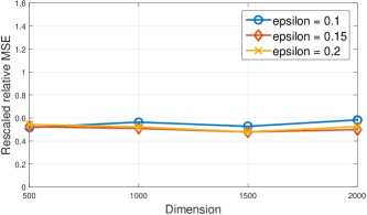
Figure 1: Simulations for Algorithm 3 showing the dependence of relative MSE on sparsity and dimension. For each parameter, we choose corresponding sample complexity $n\propto k^{2}\log(d)/\epsilon$. Different curves for $\epsilon\in\{0.1,0.15,0.2\}$ are the average of 15 trials. Consistent with the theory, the rescaled relative MSE’s are nearly independent of sparsity and dimension. Furthermore, by rescaling for different $\epsilon$, three curves have the same magnitude.

H.2 Robust sparse regression with identity covariance

We use Algorithm 1 for robust sparse regression. Similarly as in Section H.1, we use Algorithm 3 as our Robust Sparse Gradient Estimator, and leverage the Sparse PCA solver from [19]. In the simulation, we fix $d=500$, and $k=5$, hence the corresponding sample complexity is $n\propto 1/\epsilon$. However, we do not use the sample splitting technique in the simulations.

The entries of the true parameter $\bm{\beta}^{*}$ are set to be either $+1$ or $-1$, hence $\left\lVert\bm{\beta}^{*}\right\rVert_{2}^{2}=k$ is fixed. The authentic ${\bm{x}}_{i}$s are generated from $\mathcal{N}(0,\bm{I}_{d})$, and the authentic $y_{i}={\bm{x}}_{i}^{\top}\bm{\beta}^{*}+\xi_{i}$ as in Model 1.1. We set the covariates of the outliers as $A$, where $A$ is a random $\pm 1$ matrix of dimension $\epsilon n/(1-\epsilon)\times d$, and set the responses of outliers to $-A\bm{\beta}^{*}$.

To show the performance of Algorithm 1 under different settings, we use different levels of $\epsilon$ and $\sigma$ in Figure 2, and track the parameter error $\left\lVert\bm{\beta}^{t}-\bm{\beta}^{*}\right\rVert_{2}^{2}$ of Algorithm 1 in each iteration. Consistent with the theory, the algorithm displays linear convergence, and the error curves flatten out at the level of the final error. Furthermore, Algorithm 1 achieves machine precision when $\sigma^{2}=0$ in the right plot of Figure 2.

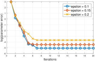
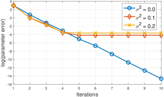
Figure 2: Empirical illustration of the linear convergence of $\log(\|\bm{\beta}^{t}-\bm{\beta}^{*}\|_{2}^{2})$ vs. iteration counts in the Algorithm 1. In all cases, we fix $k=5$, $d=500$, and choose the sample complexity $n\propto 1/\epsilon$. The left plot considers different $\epsilon$ with fixed $\sigma^{2}=0.1$. The right plot considers different $\sigma^{2}$ with fixed $\epsilon=0.1$. As expected, the convergence is linear, and flatten out at the level of the final error.

H.3 Robust sparse regression with unknown covariance matrix

Following Section H.2, we study the empirical performance of robust sparse regression with unknown covariance matrix $\bm{\Sigma}$ following from Model 5.1.

We use the same experimental setup as in Section H.2, but modify the covariance matrix to be a Toeplitz matrix with a decay $\bm{\Sigma}_{ij}=\exp^{-(i-j)^{2}}$. Under this setting, the covariance matrix is sparse, thus follows from Model 5.1. Figure 3 indicates that we have nearly the same performance as the $\bm{\Sigma}=\bm{I}_{d}$ case.

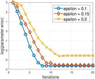
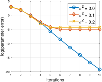
Figure 3: Empirical illustration of the linear convergence of $\log(\|\bm{\beta}^{t}-\bm{\beta}^{*}\|_{2}^{2})$ vs. iteration counts in the Algorithm 1 with unknown covariance matrix which is a Toeplitz matrix with a decay $\bm{\Sigma}_{ij}=\exp^{-(i-j)^{2}}$. The other settings are the same as Figure 2. Even though the covariance matrix is unknown, we observe similar performance in linear convergence as Figure 2.

References

- [1] Sivaraman Balakrishnan, Simon S. Du, Jerry Li, and Aarti Singh. Computationally efficient robust sparse estimation in high dimensions. In Proceedings of the 2017 Conference on Learning Theory, 2017.
- [2] Sivaraman Balakrishnan, Martin J Wainwright, and Bin Yu. Statistical guarantees for the em algorithm: From population to sample-based analysis. The Annals of Statistics, 45(1):77–120, 2017.
- [3] Afonso S. Bandeira, Edgar Dobriban, Dustin G. Mixon, and William F. Sawin. Certifying the restricted isometry property is hard. IEEE Transactions on Information Theory, 59(6):3448–3450, 2013.
- [4] Boaz Barak and David Steurer. Proofs, beliefs, and algorithms through the lens of sum-of-squares. Course notes: http://www. sumofsquares. org/public/index. html, 2016.
- [5] Kush Bhatia, Prateek Jain, and Purushottam Kar. Robust regression via hard thresholding. In Advances in Neural Information Processing Systems, pages 721–729, 2015.
- [6] Kush Bhatia, Prateek Jain, and Purushottam Kar. Consistent robust regression. In Advances in Neural Information Processing Systems, pages 2107–2116, 2017.
- [7] Peter J Bickel and Elizaveta Levina. Covariance regularization by thresholding. The Annals of Statistics, 36(6):2577–2604, 2008.
- [8] Thomas Blumensath and Mike E Davies. Iterative hard thresholding for compressed sensing. Applied and computational harmonic analysis, 27(3):265–274, 2009.
- [9] Sébastien Bubeck. Convex optimization: Algorithms and complexity. Foundations and Trends® in Machine Learning, 8(3-4):231–357, 2015.
- [10] Mengjie Chen, Chao Gao, and Zhao Ren. Robust covariance and scatter matrix estimation under huber’s contamination model. Ann. Statist., 46(5):1932–1960, 10 2018.
- [11] Yudong Chen, Constantine Caramanis, and Shie Mannor. Robust sparse regression under adversarial corruption. In International Conference on Machine Learning, pages 774–782, 2013.
- [12] Yudong Chen, Lili Su, and Jiaming Xu. Distributed statistical machine learning in adversarial settings: Byzantine gradient descent. Proceedings of the ACM on Measurement and Analysis of Computing Systems, 1(2):44, 2017.
- [13] Ilias Diakonikolas, Gautam Kamath, Daniel M Kane, Jerry Li, Ankur Moitra, and Alistair Stewart. Robust estimators in high dimensions without the computational intractability. In Foundations of Computer Science (FOCS), 2016 IEEE 57th Annual Symposium on, pages 655–664. IEEE, 2016.
- [14] Ilias Diakonikolas, Gautam Kamath, Daniel M. Kane, Jerry Li, Ankur Moitra, and Alistair Stewart. Being robust (in high dimensions) can be practical. In International Conference on Machine Learning, pages 999–1008, 2017.
- [15] Ilias Diakonikolas, Gautam Kamath, Daniel M Kane, Jerry Li, Jacob Steinhardt, and Alistair Stewart. Sever: A robust meta-algorithm for stochastic optimization. arXiv preprint arXiv:1803.02815, 2018.
- [16] Ilias Diakonikolas, Daniel M Kane, and Alistair Stewart. Statistical query lower bounds for robust estimation of high-dimensional gaussians and gaussian mixtures. In Foundations of Computer Science (FOCS), 2017 IEEE 58th Annual Symposium on, pages 73–84. IEEE, 2017.
- [17] Ilias Diakonikolas, Weihao Kong, and Alistair Stewart. Efficient algorithms and lower bounds for robust linear regression. In Proceedings of the Thirtieth Annual ACM-SIAM Symposium on Discrete Algorithms, pages 2745–2754. SIAM, 2019.
- [18] David L Donoho. Compressed sensing. IEEE Transactions on information theory, 52(4):1289–1306, 2006.
- [19] Alexandre d’Aspremont, Francis Bach, and Laurent El Ghaoui. Optimal solutions for sparse principal component analysis. Journal of Machine Learning Research, 9(Jul):1269–1294, 2008.
- [20] Noureddine El Karoui. Operator norm consistent estimation of large-dimensional sparse covariance matrices. The Annals of Statistics, 36(6):2717–2756, 2008.
- [21] Chao Gao. Robust regression via mutivariate regression depth. arXiv preprint arXiv:1702.04656, 2017.
- [22] Michael Grant, Stephen Boyd, and Yinyu Ye. Cvx: Matlab software for disciplined convex programming, 2008.
- [23] Frank R Hampel, Elvezio M Ronchetti, Peter J Rousseeuw, and Werner A Stahel. Robust statistics: the approach based on influence functions, volume 196. John Wiley & Sons, 2011.
- [24] Matthew J Holland and Kazushi Ikeda. Efficient learning with robust gradient descent. arXiv preprint arXiv:1706.00182, 2017.
- [25] Samuel B Hopkins, Tselil Schramm, Jonathan Shi, and David Steurer. Fast spectral algorithms from sum-of-squares proofs: tensor decomposition and planted sparse vectors. In Proceedings of the forty-eighth annual ACM symposium on Theory of Computing, pages 178–191. ACM, 2016.
- [26] Peter J Huber. Robust estimation of a location parameter. The annals of mathematical statistics, pages 73–101, 1964.
- [27] Peter J Huber. Robust statistics. In International Encyclopedia of Statistical Science, pages 1248–1251. Springer, 2011.
- [28] Prateek Jain, Ambuj Tewari, and Purushottam Kar. On iterative hard thresholding methods for high-dimensional m-estimation. In Advances in Neural Information Processing Systems, pages 685–693, 2014.
- [29] David S Johnson and Franco P Preparata. The densest hemisphere problem. Theoretical Computer Science, 6(1):93–107, 1978.
- [30] Sushrut Karmalkar and Eric Price. Compressed sensing with adversarial sparse noise via l1 regression. arXiv preprint arXiv:1809.08055, 2018.
- [31] Adam Klivans, Pravesh K. Kothari, and Raghu Meka. Efficient Algorithms for Outlier-Robust Regression. arXiv preprint arXiv:1803.03241, 2018.
- [32] Adam R Klivans, Philip M Long, and Rocco A Servedio. Learning halfspaces with malicious noise. Journal of Machine Learning Research, 10(Dec):2715–2740, 2009.
- [33] Kevin A Lai, Anup B Rao, and Santosh Vempala. Agnostic estimation of mean and covariance. In Foundations of Computer Science (FOCS), 2016 IEEE 57th Annual Symposium on, pages 665–674. IEEE, 2016.
- [34] Xiaodong Li. Compressed sensing and matrix completion with constant proportion of corruptions. Constructive Approximation, 37(1):73–99, 2013.
- [35] Haoyang Liu and Rina Foygel Barber. Between hard and soft thresholding: optimal iterative thresholding algorithms. arXiv preprint arXiv:1804.08841, 2018.
- [36] Liu Liu, Tianyang Li, and Constantine Caramanis. High dimensional robust -estimation: Arbitrary corruption and heavy tails. arXiv preprint arXiv:1901.08237, 2019.
- [37] Nam H Nguyen and Trac D Tran. Exact recoverability from dense corrupted observations via l1-minimization. IEEE transactions on information theory, 59(4):2017–2035, 2013.
- [38] Adarsh Prasad, Arun Sai Suggala, Sivaraman Balakrishnan, and Pradeep Ravikumar. Robust estimation via robust gradient estimation. arXiv preprint arXiv:1802.06485, 2018.
- [39] Peter J Rousseeuw and Annick M Leroy. Robust regression and outlier detection, volume 589. John wiley & sons, 2005.
- [40] Jie Shen and Ping Li. A tight bound of hard thresholding. The Journal of Machine Learning Research, 18(1):7650–7691, 2017.
- [41] Charles M Stein. Estimation of the mean of a multivariate normal distribution. The annals of Statistics, pages 1135–1151, 1981.
- [42] John W Tukey. Mathematics and the picturing of data. In Proceedings of the International Congress of Mathematicians, Vancouver, 1975, volume 2, pages 523–531, 1975.
- [43] Roman Vershynin. Introduction to the non-asymptotic analysis of random matrices. arXiv preprint arXiv:1011.3027, 2010.
- [44] Vincent Q Vu, Juhee Cho, Jing Lei, and Karl Rohe. Fantope projection and selection: A near-optimal convex relaxation of sparse PCA. In Advances in neural information processing systems, pages 2670–2678, 2013.
- [45] Martin Wainwright. High-dimensional statistics: A non-asymptotic viewpoint. Cambridge University Press, 2019.
- [46] Huan Xu, Constantine Caramanis, and Shie Mannor. Outlier-robust PCA: the high-dimensional case. IEEE transactions on information theory, 59(1):546–572, 2013.
- [47] Huan Xu, Constantine Caramanis, and Sujay Sanghavi. Robust PCA via outlier pursuit. IEEE Transactions on Information Theory, 58(5):3047–3064, 2012.
- [48] Yuchen Zhang, Martin J Wainwright, and Michael I Jordan. Lower bounds on the performance of polynomial-time algorithms for sparse linear regression. In Conference on Learning Theory, pages 921–948, 2014.