Comparison of 1D and 3D Models for the Estimation of Fractional Flow Reserve

Abstract

In this work we propose to validate the predictive capabilities of one-dimensional (1D) blood flow models with full three-dimensional (3D) models in the context of patient-specific coronary hemodynamics in hyperemic conditions. Such conditions mimic the state of coronary circulation during the acquisition of the Fractional Flow Reserve (FFR) index. Demonstrating that 1D models accurately reproduce FFR estimates obtained with 3D models has implications in the approach to computationally estimate FFR. To this end, a sample of 20 patients was employed from which 29 3D geometries of arterial trees were constructed, 9 obtained from coronary computed tomography angiography (CCTA) and 20 from intra-vascular ultrasound (IVUS). For each 3D arterial model, a 1D counterpart was generated. The same outflow and inlet pressure boundary conditions were applied to both (3D and 1D) models. In the 1D setting, pressure losses at stenoses and bifurcations were accounted for through specific lumped models. Comparisons between 1D models (FFR_1D) and 3D models (FFR_3D) were performed in terms of predicted FFR value. Compared to FFR_3D, FFR_1D resulted with a difference of 0.00$\pm$0.03 and overall predictive capability AUC, Acc, Spe, Sen, PPV and NPV of 0.97, 0.98, 0.90, 0.99, 0.82, and 0.99, with an FFR threshold of 0.8. We conclude that inexpensive FFR_1D simulations can be reliably used as a surrogate of demanding FFR_3D computations.

Introduction

Fractional Flow Reserve (FFR) is a hemodynamic index aimed at the quantification of the functional severity of a coronary artery stenosis. This index, which is calculated from pressure measurements and under hyperemic conditions, has been proposed and used to detect myocardial ischemia [26, 9], and has largely demonstrated excellent results as a diagnostic tool to defer patients with intermediate lesions to surgical procedures [27, 32, 34].

Making use of valuable information regarding anatomy and vascular geometry contained in medical images, the scientific community specialized in computational models initiated a race pursuing the paradigm of noninvasive estimation of FFR through the use of computer simulations of coronary blood flow. A myriad of different approaches using image modalities such as coronary computed tomography angiography (CCTA) [31], angiography (AX) [23], and even optical coherence tomography (OCT) [11], emerged. These approaches employ 3D models to estimate pressure losses in coronary vessels and thus to devise a strategy to predict patient-specific FFR. Such technology has been useful to improve diagnostic accuracy with respect to different traditional protocols taking the invasive measurement of FFR as gold standard [17, 22, 36]. It is important to remark that the use of 3D models carry several challenges, which range from detailed 3D lumen segmentation procedures and mesh generation to time-consuming numerical simulations in high performance computing facilities.

In turn, simplified mathematical models, either based on the 1D Navier-Stokes equations in compliant vessels [13] or based on compartmental (0D) representations [18] have been employed to study different aspects of coronary physiology. Since these models neglect fundamental aspects of the 3D physics regarding flow across geometric singularities, specific models to account for focal pressure losses are usually employed [37, 14, 24]. However, these lumped models require the definition of specific parameters which may result in a cumbersome task. Validation of 1D models by using 3D simulations as gold standard for idealized phantoms and patient-specific arterial districts such as the cerebral arteries, the aorta and major vessels were reported elsewhere [10, 15, 35, 2]. However, no validation was performed combining hyperemia, stenotic lesions and patient specific coronary territories, which are key ingredients in the computational estimation of FFR. Yet the use of 1D models to estimate FFR using CCTA or AX images has been recently proposed [28, 8, 33, 16]. It is worth noting that, in the context of coronary circulation, the validation of 1D models against 3D models has only been reported in [5], where a virtual patient population derived from a single CT scan was used. However, a comprehensive validation that accounts for large variability observed in terms of lumen geometry and hyperemic flow conditions is lacking.

The goal of this work is to demonstrate that 1D models are capable of predicting FFR (denoted FFR_1D) with a high degree of accuracy when compared with FFR predicted by 3D models (denoted FFR_3D), which is used as ground truth. To achieve this goal we make use of a sample of patients for which CCTA and IVUS images were available. After the generation of 3D models, the corresponding 1D centerlines representing the arterial topology were extracted. Then, 3D and 1D numerical simulations were performed under the assumption of hyperemic flow conditions and using appropriate boundary conditions. Several modeling scenarios are proposed from which two stand out: a scenario for practical use, and a best case scenario. The former scenario contains generic model parameters which need no tuning whatsoever. The later scenario represents the ultimate 1D modeling approach, in which several model parameters have been estimated to match data extracted from 3D models.

Material and Methods

Vascular Models

The patient sample consisted of 20 patients who were referred to CCTA and/or IVUS protocols for diagnostic or therapeutic percutaneous coronary procedure at Sírio-Libanês Hospital, São Paulo, Brazil. A total of 29 reconstructed arterial trees were available, 9 obtained from coronary computed tomography angiography (CCTA) and 20 constructed from intra-vascular ultrasound (IVUS).

CCTA images were acquired at end-diastole. Segmentation of arterial geometries from CCTA was performed using implicit deformable models [4] with tools available in the vmtk library [1]. IVUS datasets contain IVUS runs and angiographic images (AX), which were synchronized with the ECG signal during the acquisition. End-diastolic frames are gated [19] and registered [20] to construct the 3D geometry using deformable models [21]. Branches in IVUS models were manually segmented and added to the vascular model. See [6] for details on the image and mesh processing for each imaging modality.

For 3D simulations, tetrahedral finite element meshes were built using the vmtk library [1]. For 1D simulations, the centerline of each vascular model (resolution of $0.05\text{ cm}$ between points) was extracted [3]. Each point of the centerline features a cross-sectional area in correspondence with the 3D model, from which the equivalent lumen radius is computed. Figure 1 presents the workflow for constructing the 3D and the 1D models.

The clinically interrogated vessel was known for each patient, as well as the position of a hypothetical invasive FFR measurement.

0.1 3D Models

Consider a rigid vascular domain $\Omega\in\mathbb{R}^{3}$, with boundary $\Gamma$ whose outward unit normal vector is $\mathbf{n}$. The boundary is decomposed into the inlet boundary $\Gamma_{i}$, the lateral wall boundary $\Gamma_{w}$ and the $N_{o}$ outlets of the domain $\Gamma_{o}^{k}$, $k=1,\ldots,N_{o}$. Blood flow is modeled as a Newtonian fluid, therefore, the Navier-Stokes equations for incompressible flows hold

$$\begin{cases}\rho\frac{\partial\mathbf{v}}{\partial t}+\rho(\nabla\mathbf{v})\mathbf{v}+\nabla p-\mu\triangle\mathbf{v}=\mathbf{0}&\text{in }\Omega,\\ \operatorname{div}\mathbf{v}=0&\text{in }\Omega,\\ \mathbf{v}=\mathbf{0}&\text{on }\Gamma_{w},\\ -p\mathbf{n}+2\mu(\nabla\mathbf{v})^{s}\mathbf{n}=P_{\text{ao}}\mathbf{n}&\text{on }\Gamma_{i},\\ -p\mathbf{n}+2\mu(\nabla\mathbf{v})^{s}\mathbf{n}=P_{\text{out}}^{k}\mathbf{n}&\text{on }\Gamma_{o}^{k},\\ \text{with }P_{\text{out}}^{k}=P_{\text{ref}}+R_{\text{out}}^{k}\int_{\Gamma_{o}^{k}}\mathbf{v}\cdot\mathbf{n}d\Gamma&k=1,\ldots,N_{o}.\end{cases}$$ (1)

where $\mathbf{v}$ and $p$ are the velocity and pressure fields, $(\cdot)^{s}$ denotes the symmetrization operation, and $\rho$ and $\mu$ are the fluid density and dynamic viscosity, respectively. At the inlet, a reference aortic pressure $P_{\text{ao}}$ is prescribed as a Neumann boundary condition. At the outlet, resistances $R_{\text{out}}^{k}$ are used to simulate the pressure losses in the remaining vasculature, up to a reference venous pressure $P_{\text{ref}}$, and are computed as explained in [6], where the 3D finite element strategy used to find approximate solutions to this model is also described.

The flow rates through the different outlets delivered by the 3D simulation result

$$Q_{\text{out}}^{k}=\int_{\Gamma_{o}^{k}}\mathbf{v}\cdot\mathbf{n}d\Gamma\qquad k=1,\ldots,N_{o},$$ (2)

which will be later used as boundary conditions for the 1D model.

0.2 1D Models

0.2.1 Mathematical Formulation

Skeletonization of $\Omega$ yields a set of centerlines, representing arterial segments, connected through a set of junctions. Centerline coordinate is denoted by $x$. The inlet boundary $\Gamma_{i}$ is now simply denoted by the inlet point $I$, and the outlet boundaries $\Gamma_{o}^{k}$ are denoted by $O_{k}$, $k=1,\ldots,N_{o}$. Given a generic centerline of size $[0,L]$, the governing 1D equations are the following

$$\begin{cases}\frac{\partial A}{\partial t}+\frac{\partial Q}{\partial x}=0&\text{in }[0,L],\\ \frac{\partial Q}{\partial t}+\frac{\partial}{\partial x}\big{(}\frac{Q^{2}}{A}\big{)}+\frac{A}{\rho}\frac{\partial P}{\partial x}+\frac{2\varpi\pi\mu U}{\rho}=0&\text{in }[0,L],\\ P=P_{0}+\beta\big{(}\sqrt{\frac{A}{A_{0}}}-1\big{)}&\text{in }[0,L],\\ \end{cases}$$ (3)

where $Q$ is the flow rate, $A$ is the lumen cross-sectional area, $P$ is the average pressure in the lumen cross section, $U=\frac{Q}{A}$ is the cross-sectional average velocity, $\varpi$ is a parameter that characterizes the velocity profile in the 1D model, $\beta$ is an effective stiffness which characterizes the compliance of the arterial wall, $P_{0}$ is a reference external pressure for which the lumen area is $A_{0}$. Since 1D models are to be compared with rigid wall 3D models, $\beta$ is set at a high value to mimick the 1D blood flow in a quasi-rigid domain (therefore $A\approx A_{0}$). In practice, a per-case estimation of $\beta$ was performed to ensure that maximum area deviations with respect to $A_{0}$ are smaller than $1\%$.

0.2.2 Boundary Conditions

Regarding boundary conditions, the inlet pressure in the 1D model is $P_{\text{ao}}$, the same as in the 3D model. For the outflow boundary conditions, the flow rates $Q_{\text{out}}^{k}$, $k=1,\ldots,N_{o}$, which are determined from (2), are prescribed. In this manner, since the blood flow through the corresponding 3D and 1D outlets is exactly the same, we ensure the same flow distribution, and, therefore, it is possible to assess the predictive capabilities of the 1D model in determining the pressure drop along the coronary tree, and in particular at lesions, by direct comparison with the 3D model, which is regarded as the ground truth.

0.2.3 Junction Models

At junctions we consider mass conservation

$$\sum_{i=1}^{N_{j}}Q_{i}=0,$$ (4)

where $N_{j}$ is the number of converging segment. For the remaining conservation equation at junctions we consider two models. The first model is the standard junction model (S model), and consists of the standard assumption of conservation of total pressure, that is

$$P_{1}+\frac{\rho}{2}U_{1}^{2}=P_{i}+\frac{\rho}{2}U_{i}^{2}\quad i=2,\ldots,N_{j},$$ (5)

Note that $i=1$ is taken as the supplier branch, i.e. the segment that provides most of the flow to the junction. The second model is denoted dissipative junction model (D model), and consists of the junction model proposed in [24] which introduces pressure losses at junctions as follows

$$P_{1}+\frac{\rho}{2}U_{1}^{2}=P_{i}+\frac{\rho}{2}U_{i}^{2}+p_{\text{loss}}\quad i=2,\ldots,N_{j},$$ (6)

where

$$p^{\text{loss}}_{i}=K_{i}\left(\frac{1}{2}\rho u^{2}_{1}\right),$$ (7)

with $u_{1}$ the velocity in the supplier branch. Moreover, the loss coefficient $K_{i}$ is defined as

$$K_{i}=\left(2C_{i}+\frac{u^{2}_{i}}{u^{2}_{1}}-1\right)\frac{u^{2}_{i}}{u^{2}_{1}},$$ (8)

with

$$C_{i}=1-\frac{1}{\lambda_{i}\psi_{i}}\cos{\big{[}\tfrac{3}{4}(\pi-\varphi_{i})\big{]}},$$ (9)

being $\lambda_{i}=\frac{Q_{i}}{Q_{1}}$, $\psi_{i}=\frac{A_{1}}{A_{i}}$ and $\varphi_{i}=\frac{3}{4}(\pi-\phi_{i})$, where $\phi_{i}=\theta_{1}-\theta_{i}$. Here, $Q_{i}$, $A_{i}$ and $\theta_{i}$ are the flow rate, the lumen area and the angle measured from the supplier branch, for branch $i$, while $Q_{1}$, $A_{1}$ and $\theta_{1}$ stand for the same quantities in the supplier branch. This model was developed for 2D bifurcations. Equations (4)-(5) or equations (4)-(6) are complemented with Riemann invariants for outgoing waves, resulting in a non-linear system of algebraic equations. For further details see [25].

0.2.4 Stenosis Model

Stenoses are accounted for through the lumped parameter model proposed in [37], for which the pressure drop across the constriction takes the form

$$\Delta P=K_{v}\frac{\mu}{D}U+K_{t}\frac{\rho}{2}\bigg{[}\frac{A}{A_{s}}-1\bigg{]}^{2}U^{2}+K_{u}\rho L_{s}\frac{dU}{dt},$$ (10)

where $U$ and $A$ ($D$ the diameter) are the velocity and lumen area in the unobstructed part of the vessel, $L_{s}$ is the stenosis length, $A_{s}$ is the minimum stenosis area, and $K_{v}$, $K_{t}$ and $K_{u}$ are model parameters characterizing viscous, turbulent and inertial effects, respectively.

0.2.5 Numerical method

Equations (3) with appropriate boundary and coupling conditions are numerically solved using the local time stepping high-order finite volume method presented in [25], where full details of the implementation are given.

0.3 Automatic Stenosis Detection

Stenoses are detected in a fully automatic fashion to ensure reproducibility. A modified version of the algorithm proposed in [30] to detect stenotic regions in centerlines was proposed and implemented. With this procedure, the values of $A_{s}$ and $L_{s}$ in equation (10) are characterized for each stenotic lesion. See Supplementary Material for details.

0.4 Scenarios and Model Parameters

Common parameters for both models are $\rho=1.05\text{g/cm}^{3}$ and $\mu=4\text{ cP}$. For the 3D model, the only fixed parameter is $P_{\text{ref}}=10\text{ mmHg}$. For the 1D model, fixed parameters are $P_{0}=88\text{ mmHg}$, $K_{t}=1.52$, $K_{u}=1.0$ and $\varpi=11$. Patient-specific parameters are: $P_{\text{ao}}$, $R_{\text{out}}$, estimated as explained in [6], and $K_{v}$ which depends on the geometry of the lesion [29], that is

$$K_{v}=32\dfrac{0.83L_{s}+3.28\sqrt{A_{s}}}{2\sqrt{A}}\left[0.75\dfrac{A}{A_{s}}+0.25\right]^{2}.$$ (11)

The parameters that play a main role in the viscous dissipation are $\varpi$ and $K_{v}$. Since the focus of this work is given to the pressure drop predictions delivered by the 1D model, then different scenarios are proposed, with baseline parameters $\varpi^{o}=11$, as suggested in [12] for coronary flow, and $K_{v}^{o}$ determined from equation (11). These scenarios are

• Raw (R) scenario: $\varpi^{o}$, without stenosis models

• Practical (P) scenario: $\varpi^{o}$ and $K_{v}^{o}$

• Intermediate (I) scenario: $\varpi^{o}$ and $K_{v}=f_{K}K_{v}^{o}$, $f_{K}$ estimated

• Best-case (B) scenario: $\varpi=f_{\varpi}{\varpi}^{o}$ and $K_{v}=f_{K}K_{v}^{o}$, $f_{K}$ and $f_{\varpi}$ both estimated

Observe that we created the R scenario in which there are no stenoses in the models. That is, models are purely 1D, and there is no need neither to apply the stenosis detection algorithm nor to define parameters $K_{t}$, $K_{u}$, $K_{v}$. In the P scenario the stenosis detection algorithm is applied, and all parameters are defined uniformly for all stenoses in all patients. In scenarios I and B, we refer to estimated parameters, which implies that data from 3D simulations is extracted and some parameters are identified using a Kalman filter-based data assimilation approach (see [7] for details) to deliver the best possible match. Factor (or stenosis factor) $f_{K}$ is estimated to define the value of $K_{v}$ for each stenosis in each vascular network such that the pressure drop $\Delta P$ delivered by the stenosis in the 1D model matches the pressure drop obtained in that stenosis from the 3D model. Factor (or profile factor) $f_{\varpi}$ is estimated to define the value of ${\varpi}$, which defines the velocity profile for each vascular network, such that the pressure at outlet locations in the 1D model matches the pressure obtained in these outlets from the 3D simulation. For both estimates ($f_{K}$ and $f_{\varpi}$), the cost functionals used are the time-averaged errors along a single cardiac cycle.

Scenarios I and B are reported because they feature the best achievable results in terms of 1D modeling. In fact, parameters in these cases are stenosis-specific ($K_{v}$) and patient-specific ($\varpi$) and constructed to match data from 3D simulations.

These four scenarios are combined with the two junctions models: S (standard, see equation (5)) and D (dissipative, see equation (6)) for a total of eight scenarios, denoted by $\text{Y}_{\text{X}}$, $\text{Y}\in\{\text{R},\text{P},\text{I},\text{B}\}$ and $\text{X}\in\{\text{S},\text{D}\}$.

0.5 Data Analysis and Comparisons

The value of FFR_3D and FFR_1D predicted by the different scenarios are compared at four relevant locations in each network. These locations correspond to major vessels (left anterior descending, circumflex, ramus intermedius and right coronary arteries) at locations $\ell_{4\text{P}}=\{\frac{\ell}{4},\frac{\ell}{2},\frac{3\ell}{4},\ell\}$, where $\ell$ is the total length of the vessel. Also, the location of invasive FFR measurement is denoted by $\ell_{\text{FFR }}$.

Comparisons are reported using mean and standard deviation of the values and discrepancies, Bland-Altman analysis ($m_{\text{BA}}\pm\text{SD}_{\text{BA}}$). Pearson’s correlation coefficient $r$, as well as coefficients of the linear approximation $\text{FFR\textsubscript{1D}}=a\text{FFR\textsubscript{3D}}+b$ are also reported. A cut-off value of $\text{FFR\textsubscript{3D}}=0.8$ is used to identify functional stenoses, and taking FFR_3D as ground truth, the prevalence (Prev), and classification indexes such as the area under the receiver operating characteristic curve (AUC), accuracy (Acc), sensitivity (Sen), specificity (Spe), positive predictive value (PPV) and negative predictive value (NPV) are calculated for each one of the different 1D scenarios considered in this work.

1 Results

Table 1 presents the statistical comparison between the stenotic pressure drop in the 3D model and the stenotic pressure drops as predicted by all the 1D scenarios described in Section 0.4. The statistics of the stenosis morphology defined by the automatic algorithm explained in Section 0.3 is also reported, where $\frac{A_{s}}{A}$ is the severity and $L_{s}$ the stenosis length, see equations (10) and (11). Also, the Reynolds number computed in the 3D model is given as the average between the inlet and outlet Reynolds numbers. In the cases of scenarios I and B, the statistics of the value of the stenosis factor $f_{K}$ estimated using the Kalman filter is given. Finally, in the B scenario, the statistics of the profile factor $f_{\varpi}$ estimated using the Kalman filter is reported.

Table 2 reports the statistical analysis of the results at $\ell_{4\text{P}}$ and $\ell_{\text{FFR }}$ locations, summarizing the performance of the eight scenarios involving 1D models with respect to the ground truth prediction of FFR_3D.

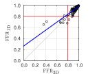
(a) Scenario $\text{R}_{\text{D}}$

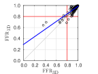
(b) Scenario $\text{R}_{\text{S}}$

(c) Scenario $\text{P}_{\text{D}}$

(d) Scenario $\text{P}_{\text{S}}$

(e) Scenario $\text{I}_{\text{D}}$

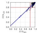
(f) Scenario $\text{I}_{\text{S}}$

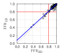
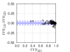
(g) Scenario $\text{B}_{\text{D}}$

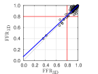
(h) Scenario $\text{B}_{\text{S}}$

Figure 2: Scatter and Bland-Altman plots featuring comparison between the gold standard FFR_3D and FFR_1D for different scenarios, $\text{Y}_{\text{X}}$, $\text{Y}\in\{\text{R},\text{P},\text{I},\text{B}\}$ and $\text{X}\in\{\text{S},\text{D}\}$, with R: raw, P: practical, I: intermediate, B: best, S: standard junction and D: dissipative junction. Results correspond to four locations, $\ell_{4\text{P}}$, in the interrogated vessels.

Figure 2 displays the scatter plot and the Bland-Altman plots for the comparison between FFR_3D, the gold standard, and FFR_1D as given by the eight different scenarios.

Discussion

Inspecting the results reported in Table 2 at the four locations $\ell_{4\text{P}}$, we observe that the all 1D model scenarios provide excellent classification capabilities when compared to the 3D model. Moreover, almost no bias and a small standard deviation are obtained for the difference $\text{FFR\textsubscript{1D}}-\text{FFR\textsubscript{3D}}$. Overall, considering the junctions as dissipative (model D), instead of standard (model S), does not bring substantial improvements neither to the correlation coefficients ($a,b,r,m_{\text{BA}},\text{SD}_{\text{BA}}$) nor to the classification indexes (AUC, Acc, Sen, Spe, PPV, NPV). More in detail, we note that the plain 1D model (scenarios $\text{R}_{\text{D}}$ or $\text{R}_{\text{S}}$) provides the poorest correlation with the 3D model (coefficients of linear regression $a=0.72$, $b=0.26$, $r=0.88$ for $\text{R}_{\text{D}}$). By adding the stenosis model with a one-fits-all strategy for the parameter calibration (scenarios $\text{P}_{\text{D}}$ or $\text{P}_{\text{S}}$), the correlation coefficients significantly improve ($a=0.96$, $b=0.03$, $r=0.95$ for $\text{P}_{\text{D}}$). This can also be appreciated in Figure 2, where the alignment of the point cloud around the $45^{\circ}$ line is clear. In such plot, the correction of some outliers is also noticeable. As a consequence, the use of stenosis models is mandatory to have the best the 1D modeling realm.

Moreover, notwithstanding the setting of stenosis-specific parameters tuned with 3D data brings some improvements, there is no considerable gain in the correlation coefficients ($a=0.97$, $b=0.03$, $r=0.96$ for $\text{I}_{\text{D}}$), while classification indexes remain invariant. Even in the best case scenario in which we further estimate the velocity profile such that 1D terminal pressures match those of 3D models, there is no relevant improvement in the model capabilities. The stenosis parameter estimated from 3D data resulted in average very close to the unit value (see Table 1) which was taken in the one-fits-all approach, and as suggested in the original contribution [37].

It is important to stress that the comparisons presented here exclusively focuse on the ability of 1D models to predict pressure drops $\Delta P$ in stenotic lesions. This has been achieved by setting the same flow rate boundary conditions extracted from the 3D models to the 1D counterparts, guaranteeing the consistency in the flow regime in among the models. The discrepancy in the stenotic $\Delta P$ estimation is also observed in Table 1. While the plain 1D model (scenarios $\text{R}_{\text{D}}$ or $\text{R}_{\text{S}}$) underestimates the $\Delta P$, the inclusion of stenosis models yields larger $\Delta P$, rendering the alignment in the correlation line seen in Figure 2. On the one hand, regarding the lesion-specific parameter $K_{v}$ estimated from 3D data (scenarios I and B), it is remarkable that, in average, it results very close to the unit value (i.e. $f_{K}=0.97\pm 0.51$), close to the value chosen for the one-fits-all approach in scenario P (theoretically $f_{K}=1$). On the other hand, regarding the characterization of the velocity profile given by network-specific parameter $\varpi$, the estimation using 3D data indicates that there is room for improvement (i.e. $f_{\varpi}=0.74\pm 0.16$, model D) in order to improve the selection criterion for such parameter.

Analyzing the prediction of FFR in clinically relevant locations $\ell_{\text{FFR}}$ (see Table 2), we observe that both the correlation coefficients and the classification indexes continue to be excellent, and the AUC index grows almost to a perfect unitary value. Particularly, the only low value is obtained for the PPV, which is in part a consequence of the low prevalence sample. However, in the best case scenarios (scenarios $\text{B}_{\text{D}}$ and $\text{B}_{\text{S}}$) demonstrate that, when properly tuned, 1D models provide an exact match with 3D models in term of diagnostic capabilities. Furthermore, at these clinically relevant locations, since in average they are more distally placed, cumulative effect of upstream junctions causes the dissipative junction (scenarios D) to outperform the standard junction (scenarios S). Therefore, our recommendation is to employ this junction model.

The relatively low prevalence of positive FFR_3D values in the $\ell_{4\text{P}}$ population, equal to 0.06, might raise concern as whether this fact is being favorable to validating our working hypothesis on the ability of 1D simulations to match 3D results. In order to rule out such concern we considered an alternative population $\hat{\ell}_{4\text{P}}$ in which we only included the points of $\ell_{4\text{P}}$ for vessels in which at least one of its points had a FFR_3D$<0.85$. In that case, the number of sampled points is 36, with a prevalence of 0.28. Statistics for all scenarios are consisted between populations $\ell_{4\text{P}}$ and $\hat{\ell}_{4\text{P}}$. Particularly, results for scenario $\text{P}_{\text{D}}$ are: mean difference of $0.01\pm 0.04$, significant correlation of 0.96, slope of 0.97 and intercept of 0.03 for the linear regression and overall AUC, accuracy, sensitivity, specificity, positive predictive value, and negative predictive value of 0.98, 0.92, 0.90, 0.92, 0.82, 0.96. Comparison of these results with the ones reported in Table 2 for the same scenario show that considerations about the accuracy of 1D simulations for FFR prediction remain valid.

In a nutshell, practical scenarios making use of one-fits-all stenosis parameters are sufficient for an excellent estimation of the pressure drop occurring as predicted by 3D simulations. The use of dissipative junctions is not mandatory, although it slightly improves the capabilities of FFR_1D, with more gains at clinically relevant locations.

Moreover, 1D models only require the use of workstations which are easily available in the medical facilities, while 3D models necessarily make use of clusters of high performance computers which poses an unrealistic scenario in clinical routine.

Final Remarks

The results reported in this work indicate that FFR_1D simulations can be reliable surrogates of FFR_3D models to assess functional significance of coronary stenoses. Even if 1D models must be endowed with stenoses models to effectively predict pressure drops in lesions, a one-fits-all strategy to set up stenoses parameters rendered excellent predictive capabilities in terms of classification indexes when regarding the FFR_3D as the ground truth. Adopting such practical strategy, and adding dissipative junctions, when compared to FFR_3D, FFR_1D renders a mean difference of $0.00\pm 0.03$ ($-0.02\pm 0.05$), and overall accuracy, sensitivity, specificity, positive predictive value, and negative predictive value of 0.98, 0.90, 0.99, 0.82, and 0.99 (0.97, 1.00, 0.97, 0.75, and 1.00), respectively, to detect significant stenoses at several locations in the coronary network (at clinically relevant locations).

Remarkably, it has been possible to show that, in the best case scenario conceived by setting properly calibrated stenoses parameters, the FFR_1D perfectly matched the classification given by FFR_3D.

Even if the present results have been obtained for a exploratory sample of patients, the results constitute a first validation survey to test the hypothesis that inexpensive FFR_1D can be reliably used instead of FFR_3D simulations. As a matter of fact, FFR_1D has the benefit of requiring substantial less time and computational resources than FFR_3D, which makes this approach affordable in clinical routine. Having demonstrated that the FFR_1D concept is feasible, the next step consists in translating this FFR_1D tool into the clinic by performing clinical studies.

Author contributions statement

Must include all authors, identified by initials, for example: P.J.B., C.A.B., L.O.M. and R.A.F. conceived the experiment(s), C.G.B. and P.A.L. collected the data, C.A.B. and G.D.M.T. processed the data, C.A.B. and L.O.M. conducted the experiment(s), P.J.B., C.A.B., L.O.M. and R.A.F. analysed the results. All authors reviewed the manuscript.

Additional information

Data availability statement: The data that support the findings of this study are available on request from the corresponding author [PJB]. The data are not publicly available due to privacy restrictions of research participants.

Competing financial interests: The authors do not have competing financial interests with regards to the study and results presented in this work.

Figure 1: Workflow for the construction of vascular models. Image segmentation produces 3D vascular geometries which are processed to retrieve the 1D centerline geometry. Lumen area is given at each centerline point and bifurcation (yellow) and stenoses (red) masks are applied when necessary. Model scenarios are: R (raw): 1D model with no stenoses and known dissipation parameter $\varpi^{o}$, P (practical): idem R scenario, but 1D model includes stenoses with known stenosis parameter $K_{v}^{o}$, I (intermediate): idem P scenario, but parameters $K_{v}$ are estimated using stenosis drop pressures $\Delta p$ at the corresponding lesions from 3D simulations, B (best-case): idem I scenario, but dissipation parameter $\varpi$ is estimated using outlet pressures $p_{i},i=1,\ldots,N_{o}$ from 3D simulations.

Junction	$\Delta P$ $[\text{mmHg}]$	1D scenarios $\Delta P$ $[\text{mmHg}]$
Model	3D	R†: raw	P†:practical	I†: intermediate	B: best
D	6.75$\pm$9.08	5.35$\pm$4.29	5.52$\pm$6.58	5.25$\pm$6.54	5.16$\pm$6.56
S		5.34$\pm$4.28	5.52$\pm$6.58	5.25$\pm$6.54	5.18$\pm$6.55

Junction	$\frac{A_{s}}{A}$	$L_{s}$ $[\text{cm}]$	Re	$f_{K}$	$f_{\varpi}$
Model				scen. $\text{I},\text{B}$	scen. B
D	0.50$\pm$0.13	0.55$\pm$0.37	185$\pm$94	0.97$\pm$0.51	0.74$\pm$0.16
S				0.97$\pm$0.51	0.76$\pm$0.22

Table 1: Comparison of stenotic pressure drop ($\Delta P$) between the 3D model and all 1D scenarios (for both junction models, D: dissipative and S: standard), in $[\text{mmHg}]$, for all stenoses. Marker ^† indicates scenarios with $p>0.05$ in the paired U-Test, meaning that no significant differences between $\Delta P$ of 1D and 3D predictions was found. $\frac{A_{s}}{A}$: stenosis degree, $L_{s}$: stenosis length; Re: Reynolds number; $f_{K}$: stenosis factor estimated by the Kalman filter; $f_{\varpi}$: velocity factor estimated by the Kalman filter. Note that $f_{\varpi}$ statistics are computed over $n=6$ computational models for which at least one stenoses was detected. The remaining statistics were computed using $n=15$ stenosis elements.

	Scenario		Linear approx.		Corr.	$\text{FFR\textsubscript{1D}}-\text{FFR\textsubscript{3D}}$	Prediction value of FFR1D vs. FFR3D
			$a$	$b$	$r$	$m_{\text{BA}}\pm\text{SD}_{\text{BA}}$	AUC	Acc	Sen	Spe	PPV	NPV
Location of comparison	$\ell_{4\text{P}}$ ($n=156$)	$\text{R}_{\text{D}}$	0.72	0.26	0.88	0.00$\pm$0.04†	0.97	0.98	0.80	0.99	0.89	0.99
		$\text{P}_{\text{D}}$	0.96	0.03	0.95	0.00$\pm$0.03†	0.97	0.98	0.90	0.99	0.82	0.99
		$\text{I}_{\text{D}}$	0.97	0.03	0.96	0.00$\pm$0.03†	0.97	0.98	0.90	0.99	0.82	0.99
		$\text{B}_{\text{D}}$	0.92	0.08	0.96	0.00$\pm$0.02	0.96	0.99	0.90	1.00	1.00	0.99
		$\text{R}_{\text{S}}$	0.69	0.29	0.87	0.01$\pm$0.04†	0.97	0.98	0.80	0.99	0.89	0.99
		$\text{P}_{\text{S}}$	0.94	0.06	0.94	0.00$\pm$0.03†	0.97	0.98	0.90	0.99	0.82	0.99
		$\text{I}_{\text{S}}$	0.95	0.05	0.94	0.00$\pm$0.03†	0.98	0.99	0.90	0.99	0.90	0.99
		$\text{B}_{\text{S}}$	0.93	0.07	0.95	0.00$\pm$0.03	0.95	0.99	0.90	1.00	1.00	0.99
	$\ell_{\text{FFR}}$ ($n=32$)	$\text{R}_{\text{D}}$	0.70	0.26	0.80	-0.01$\pm$0.07	0.99	0.97	1.00	0.97	0.75	1.00
		$\text{P}_{\text{D}}$	1.01	-0.03	0.92	-0.02$\pm$0.05	0.99	0.97	1.00	0.97	0.75	1.00
		$\text{I}_{\text{D}}$	1.02	-0.04	0.92	-0.02$\pm$0.05	0.99	0.97	1.00	0.97	0.75	1.00
		$\text{B}_{\text{D}}$	1.02	-0.03	0.92	-0.01$\pm$0.05†	1.00	1.00	1.00	1.00	1.00	1.00
		$\text{R}_{\text{S}}$	0.69	0.28	0.79	-0.01$\pm$0.07†	0.99	0.94	0.67	0.97	0.67	0.97
		$\text{P}_{\text{S}}$	1.00	-0.01	0.91	-0.02$\pm$0.05†	0.99	0.94	0.67	0.97	0.67	0.97
		$\text{I}_{\text{S}}$	1.01	-0.03	0.91	-0.02$\pm$0.06†	0.99	0.94	0.67	0.97	0.67	0.97
		$\text{B}_{\text{S}}$	1.04	-0.04	0.93	-0.01$\pm$0.05†	1.00	0.97	0.67	1.00	1.00	0.97

Table 2: Statistical results of predictive capabilities of FFR_1D when compared with FFR_3D for the different scenarios $\text{Y}_{\text{X}}$, $\text{Y}\in\{\text{R},\text{P},\text{I},\text{B}\}$ and $\text{X}\in\{\text{S},\text{D}\}$, with R: raw, P: practical, I: intermediate, B: best, S: standard junction and D: dissipative junction. Values of FFR compared at four locations, $\ell_{4\text{P}}$, in the interrogated vessel as well as at the clinically relevant location for diagnosis, $\ell_{\text{FFR }}$. Sample sizes are obtained from the 29 computational models. Prevalence of functional stenoses according to FFR_3D: $0.06$ for $\ell_{4\text{P}}$ and $0.09$ for $\ell_{\text{FFR}}$. Linear approximation coefficients defined by $a$ and $b$. $r$: Pearson’s correlation coefficient ($p<0.05$ for all models). $m_{\text{BA}}\pm\text{SD}_{\text{BA}}$: mean and standard deviation of Bland-Altman analysis for the difference $\text{FFR\textsubscript{1D}}-\text{FFR\textsubscript{3D}}$. Marker ^† indicates correlation ($p\geq 0.05$) between 1D and 3D models. Predicted values (AUC, Acc, Sen, Spe, PPV, NPV) computed using FFR_3D as gold standard and a cut-off value of $\text{FFR}\geq 0.8$.

References

- [1] The vascular modeling toolkit website. URL www.vmtk.org.
- Alastruey et al. [2016] Alastruey, J., Xiao, N., Fok, H., Schaeffter, T., and Figueroa, C. A. On the impact of modelling assumptions in multi-scale, subject-specific models of aortic haemodynamics. Journal of The Royal Society Interface, 13(119):20160073, 2016.
- Antiga et al. [2003] Antiga, L., Ene-Iordache, B., and Remuzzi, A. Computational geometry for patient-specific reconstruction and meshing of blood vessels from MR and CT angiography. IEEE Transactions on Medical Imaging, 22(5):674–684, 2003.
- Antiga et al. [2008] Antiga, L., Piccinelli, M., Botti, L., Ene-Iordache, B., Remuzzi, A., and Steinman, D. An image-based modeling framework for patient-specific computational hemodynamics. Medical & Biological Engineering & Computing, 46:1097–1112, 2008.
- Boileau et al. [2018] Boileau, E., Pant, S., Roobottom, C., Sazonov, I., Deng, J., Xie, X., and Nithiarasu, P. Estimating the accuracy of a reduced-order model for the calculation of fractional flow reserve (FFR). International Journal for Numerical Methods in Biomedical Engineering, 34:e2908, 2018.
- Bulant et al. [2017] Bulant, C., Blanco, P., Maso Talou, G., Guedes Bezerra, C., Lemos, P., and Feijóo, R. A head-to-head comparison between CCTA- and IVUS-derived coronary blood flow models. Journal of Biomechanics, 51:65–76, 2017.
- Caiazzo et al. [2017] Caiazzo, A., Caforio, F., Montecinos, G., Müller, L., Blanco, P., and Toro, E. Assessment of reduced-order unscented Kalman filter for parameter identification in one-dimensional blood flow models using experimental data. International Journal for Numerical Methods in Biomedical Engineering, 33:e2843, 2017.
- Coenen et al. [2014] Coenen, A., Lubbers, M. M., Kurata, A., Kono, A., Dedic, A., Chelu, R. G., Dijkshoorn, M. L., Gijsen, F. J., Ouhlous, M., van Geuns, R.-J. M., and others. Fractional flow reserve computed from noninvasive CT angiography data: diagnostic performance of an on-site clinician-operated computational fluid dynamics algorithm. Radiology, 274(3):674–683, 2014.
- De Bruyne et al. [2000] De Bruyne, B., Pijls, N. H. J., Heyndrickx, G. R., Hodeige, D., Kirkeeide, R., and Gould, K. L. Pressure-Derived Fractional Flow Reserve to Assess Serial Epicardial Stenoses : Theoretical Basis and Animal Validation. Circulation, 101(15):1840–1847, 2000.
- Grinberg et al. [2011] Grinberg, L., Cheever, E., Anor, T., Madsen, J. R., and Karniadakis, G. E. Modeling Blood Flow Circulation in Intracranial Arterial Networks: A Comparative 3D/1D Simulation Study. Annals of Biomedical Engineering, 39(1):297–309, 2011.
- Ha et al. [2016] Ha, J., Kim, J.-S., Lim, J., Kim, G., Lee, S., Lee, J. S., Shin, D.-H., Kim, B.-K., Ko, Y.-G., Choi, D., and others. Assessing Computational Fractional Flow Reserve From Optical Coherence Tomography in Patients With Intermediate Coronary Stenosis in the Left Anterior Descending Artery. Circulation: Cardiovascular Interventions, 9(8):e003613, 2016.
- Hunter [1972] Hunter, P. J. Numerical simulation of arterial blood flow. Master’s Thesis, The University of Auckland, Auckland, 1972.
- Huo and Kassab [2007] Huo, Y. and Kassab, G. S. A hybrid one-dimensional/Womersley model of pulsatile blood flow in the entire coronary arterial tree. AJP: Heart and Circulatory Physiology, 292(6):H2623–H2633, 2007.
- Huo et al. [2012] Huo, Y., Svendsen, M., Choy, J. S., Zhang, Z.-D., and Kassab, G. S. A validated predictive model of coronary fractional flow reserve. Journal of The Royal Society Interface, 9(71):1325–1338, 2012.
- Jonášová et al. [2014] Jonášová, A., Bublík, O., and Vimmr, J. A comparative study of 1D and 3D hemodynamics in patient-specific hepatic portal vein networks. Applied and Computational Mechanics, 8(2), 2014.
- Ko et al. [2016] Ko, B. S., Cameron, J. D., Munnur, R. K., Wong, D. T., Fujisawa, Y., Sakaguchi, T., Hirohata, K., Hislop-Jambrich, J., Fujimoto, S., Takamura, K., Crossett, M., Leung, M., Kuganesan, A., Malaiapan, Y., Nasis, A., Troupis, J., Meredith, I. T., and Seneviratne, S. K. Noninvasive CT-Derived FFR Based on Structural and Fluid Analysis. JACC: Cardiovascular Imaging, October 2016.
- Koo et al. [2011] Koo, B.-K., Erglis, A., Doh, J.-H., Daniels, D. V., Jegere, S., Kim, H.-S., Dunning, A., DeFrance, T., Lansky, A., Leipsic, J., and Min, J. K. Diagnosis of Ischemia-Causing Coronary Stenoses by Noninvasive Fractional Flow Reserve Computed From Coronary Computed Tomographic Angiograms. Journal of the American College of Cardiology, 58(19):1989–1997, 2011.
- Maasrani et al. [2008] Maasrani, M., Verhoye, J.-P., Corbineau, H., and Drochon, A. Analog Electrical Model of the Coronary Circulation in Case of Multiple Revascularizations. Annals of Biomedical Engineering, 36(7):1163–1174, 2008.
- Maso Talou et al. [2015] Maso Talou, G., Larrabide, I., Blanco, P., Guedes Bezerra, C., Lemos, P., and Feijóo, R. Improving cardiac phase extraction in IVUS studies by integration of gating methods. IEEE Transactions on Biomedical Engineering, 62:2867–2877, 2015.
- Maso Talou et al. [2017] Maso Talou, G., Blanco, P., Larrabide, I., Guedes Bezerra, C., Lemos, P., and Feijóo, R. Registration methods for IVUS: transversal and longitudinal transducer motion compensation. IEEE Transactions on Biomedical Engineering, 64:890–903, 2017.
- Maso Talou [2013] Maso Talou, G. IVUS images segmentation driven by active contours and spacio-temporal reconstruction of the coronary vessels aided by angiographies. Master’s thesis, National Laboratory for Scientific Computing, Petrópolis, Brazil, 2013.
- Min et al. [2012] Min, J. K., Leipsic, J., Pencina, M. J., Berman, D. S., Koo, B.-K., van Mieghem, C., Erglis, A., Lin, F. Y., Dunning, A. M., Apruzzese, P., Budoff, M. J., Cole, J. H., Jaffer, F. A., Leon, M. B., Malpeso, J., Mancini, G. B. J., Park, S.-J., Schwartz, R. S., Shaw, L. J., and Mauri, L. Diagnostic Accuracy of Fractional Flow Reserve From Anatomic CT Angiography. JAMA, 308(12):1237, 2012.
- Morris et al. [2013] Morris, P. D., Ryan, D., Morton, A. C., Lycett, R., Lawford, P. V., Hose, D. R., and Gunn, J. P. Virtual Fractional Flow Reserve From Coronary Angiography: Modeling the Significance of Coronary Lesions. JACC: Cardiovascular Interventions, 6(2):149–157, 2013.
- Mynard and Valen-Sendstad [2015] Mynard, J. and Valen-Sendstad, K. A unified method for estimating pressure losses at vascular junctions. International Journal for Numerical Methods in Biomedical Engineering, 31:e02717, 2015.
- Müller et al. [2016] Müller, L. O., Blanco, P. J., Watanabe, S. M., and Feijóo, R. A. A high-order local time stepping finite volume solver for one-dimensional blood flow simulations: application to the ADAN model. International Journal for Numerical Methods in Biomedical Engineering, 32(10):e02761, October 2016.
- Pijls et al. [1996] Pijls, N. H., de Bruyne, B., Peels, K., van der Voort, P. H., Bonnier, H. J., Bartunek, J., and Koolen, J. J. Measurement of fractional flow reserve to assess the functional severity of coronary-artery stenoses. New England Journal of Medicine, 334(26):1703–1708, 1996.
- Pijls et al. [2007] Pijls, N. H., van Schaardenburgh, P., Manoharan, G., Boersma, E., Bech, J.-W., van’t Veer, M., Bär, F., Hoorntje, J., Koolen, J., Wijns, W., and de Bruyne, B. Percutaneous Coronary Intervention of Functionally Nonsignificant Stenosis. Journal of the American College of Cardiology, 49(21):2105–2111, 2007.
- Renker et al. [2014] Renker, M., Schoepf, U. J., Wang, R., Meinel, F. G., Rier, J. D., Bayer, R. R., Möllmann, H., Hamm, C. W., Steinberg, D. H., and Baumann, S. Comparison of Diagnostic Value of a Novel Noninvasive Coronary Computed Tomography Angiography Method Versus Standard Coronary Angiography for Assessing Fractional Flow Reserve. The American Journal of Cardiology, 114(9):1303–1308, November 2014.
- Seeley and Young [1976] Seeley, B. D. and Young, D. F. Effect of geometry on pressure losses across models of arterial stenoses. Journal of biomechanics, 9(7):439–448, 1976.
- Shahzad et al. [2013] Shahzad, R., Kirişli, H., Metz, C., Tang, H., Schaap, M., van Vliet, L., Niessen, W., and van Walsum, T. Automatic segmentation, detection and quantification of coronary artery stenoses on CTA. The International Journal of Cardiovascular Imaging, 29(8):1847–1859, December 2013. ISSN 1569-5794, 1573-0743. 10.1007/s10554-013-0271-1. URL http://link.springer.com/10.1007/s10554-013-0271-1.
- Taylor et al. [2013] Taylor, C. A., Fonte, T. A., and Min, J. K. Computational Fluid Dynamics Applied to Cardiac Computed Tomography for Noninvasive Quantification of Fractional Flow Reserve. Journal of the American College of Cardiology, 61(22):2233–2241, 2013.
- Tonino et al. [2009] Tonino, P. A. L., De Bruyne, B., Pijls, N. H. J., Siebert, U., Ikeno, F., van’ t Veer, M., Klauss, V., Manoharan, G., Engstrøm, T., Oldroyd, K. G., Ver Lee, P. N., MacCarthy, P. A., Fearon, W. F., and FAME Study Investigators. Fractional flow reserve versus angiography for guiding percutaneous coronary intervention. The New England journal of medicine, 360(3):213–224, January 2009. ISSN 1533-4406. 10.1056/NEJMoa0807611.
- Tröbs et al. [2016] Tröbs, M., Achenbach, S., Röther, J., Redel, T., Scheuering, M., Winneberger, D., Klingenbeck, K., Itu, L., Passerini, T., Kamen, A., Sharma, P., Comaniciu, D., and Schlundt, C. Comparison of Fractional Flow Reserve Based on Computational Fluid Dynamics Modeling Using Coronary Angiographic Vessel Morphology Versus Invasively Measured Fractional Flow Reserve. The American Journal of Cardiology, 117(1):29–35, January 2016.
- van Nunen et al. [2015] van Nunen, L. X., Zimmermann, F. M., Tonino, P. A. L., Barbato, E., Baumbach, A., Engstrøm, T., Klauss, V., MacCarthy, P. A., Manoharan, G., Oldroyd, K. G., Ver Lee, P. N., van’t Veer, M., Fearon, W. F., De Bruyne, B., and Pijls, N. H. J. Fractional flow reserve versus angiography for guidance of PCI in patients with multivessel coronary artery disease (FAME): 5-year follow-up of a randomised controlled trial. The Lancet, 386(10006):1853–1860, November 2015. ISSN 01406736. 10.1016/S0140-6736(15)00057-4. URL http://linkinghub.elsevier.com/retrieve/pii/S0140673615000574.
- Xiao et al. [2014] Xiao, N., Alastruey, J., and Alberto Figueroa, C. A systematic comparison between 1-D and 3-D hemodynamics in compliant arterial models. International Journal for Numerical Methods in Biomedical Engineering, 30(2):204–231, 2014.
- Yoon et al. [2012] Yoon, Y. E., Choi, J.-H., Kim, J.-H., Park, K.-W., Doh, J.-H., Kim, Y.-J., Koo, B.-K., Min, J. K., Erglis, A., Gwon, H.-C., Choe, Y. H., Choi, D.-J., Kim, H.-S., Oh, B.-H., and Park, Y.-B. Noninvasive Diagnosis of Ischemia-Causing Coronary Stenosis Using CT Angiography. JACC: Cardiovascular Imaging, 5(11):1088–1096, 2012.
- Young and Tsai [1973] Young, D. and Tsai, F. Flow characteristics in models of arterial stenoses. II. Unsteady flow. Journal of Biomechanics, pages 547–559, 1973.
Acknowledgements
Acknowledgements should be brief, and should not include thanks to anonymous referees and editors, or effusive comments. Grant or contribution numbers may be acknowledged.