Supporting Information
Optimal nanoparticle forces, torques, and illumination fields

I Time-reversal properties of energy/momentum flux operators

In the main text, we saw that energy/momentum quantities of interest, such as absorbed power, force, or torque, can generally be written for a field $\psi$ as quadratic forms

$$Q=\int_{S}\psi^{\dagger}\mathcal{Q}\psi,$$ (S1)

where $\mathcal{Q}$ is a Hermitian operator determined by the Poyting vector or the electromagnetic stress tensor. Here, we use the fact that $\mathcal{Q}$ represents energy or momentum flow to assert that $\mathcal{Q}$ must satisfy a general time-reversal expression.

Consider a total field that is purely outgoing: $\psi=\mathbb{V}_{+}\bm{\mathbf{c}}$. Then $Q$ would be given by

$$Q=\bm{\mathbf{c}}^{\dagger}\left(\int_{S}\mathbb{V}_{+}^{\dagger}\mathcal{Q}\mathbb{V}_{+}\right)\bm{\mathbf{c}}$$ (S2)

If we time-reverse the fields, $\mathbb{V}_{+}\rightarrow\mathbb{V}_{-}=\mathcal{P}\overline{\mathbb{V}_{+}}$, then the quantity $Q$ must go to its negative (energy/momentum flows in the opposite direction):

$$-Q =\bm{\mathbf{c}}^{\dagger}\left(\int_{S}\mathbb{V}_{+}^{T}\mathcal{P}\mathcal{Q}\mathcal{P}\overline{\mathbb{V}_{+}}\right)\bm{\mathbf{c}}$$

$$=\bm{\mathbf{c}}^{\dagger}\left(\int_{S}\mathbb{V}_{+}^{\dagger}\mathcal{P}\mathcal{Q}^{T}\mathcal{P}\mathbb{V}_{+}\right)\bm{\mathbf{c}}.$$ (S3)

Since Eq. (S2) and Eq. (S3) apply for any $\bm{\mathbf{c}}$ and any $\mathbb{V}_{+/-}$, we have the relation

$$\mathcal{Q}=-\mathcal{P}\mathcal{Q}^{T}\mathcal{P}.$$ (S4)

From Eq. (S4), it is straightforward to show that, as argued in the main text, that the incoming/outgoing channels carry equal and opposite energy/momentum:

$$\int_{S}\mathbb{V}_{+}^{\dagger}\mathcal{Q}\mathbb{V}_{+}=-\int_{S}\mathbb{V}_{-}^{\dagger}\mathcal{Q}\mathbb{V}_{-}.$$ (S5)

II Quadratic forms

First, we show that we can write the flux rates of power, linear momentum, and angular momentum through any surface $S$ as the quadratic form given by Eq. (S1) and repeated here,

$$Q=\int_{S}\psi^{\dagger}\mathcal{Q}\psi,$$ (S6)

II.1 Power

Assuming an outward normal $\hat{\bm{\mathbf{n}}}$ on some surface $S$, net power flow in a field $\psi$ is given by the Poynting vector, which can be written in six-vector notation as

$$P =\int_{S}\psi^{\dagger}\left(-\frac{1}{4}\Theta\right)\psi,$$ (S7)

where $\Theta$ is the real-symmetric matrix,

$$\Theta=\begin{pmatrix}&-\hat{\bm{\mathbf{n}}}\times\\ \hat{\bm{\mathbf{n}}}\times&\end{pmatrix}.$$ (S8)

II.2 Linear momentum

The flux of linear momentum through a surface is determined by a surface integral of the Maxwell stress tensor, which is $\overline{\overline{\bm{\sigma}}}=\left[\mathbf{E}\mathbf{E}^{\dagger}-\frac{1}{2}\bm{\mathcal{I}}\left(\mathbf{E}^{\dagger}\mathbf{E}\right)\right]+\left[\mathbf{H}\mathbf{H}^{\dagger}-\frac{1}{2}\bm{\mathcal{I}}\left(\mathbf{H}^{\dagger}\mathbf{H}\right)\right]$ (for $\varepsilon_{0}=\mu_{0}=1$). The linear-momentum flux along a given direction, denoted $\hat{\bm{\mathbf{x}}}$, is given by

$$\bm{\mathbf{P}}\cdot\hat{\bm{\mathbf{x}}}=\frac{1}{2}\operatorname{Re}\int_{S}\hat{\bm{\mathbf{x}}}\cdot\left\{\left[\mathbf{E}\mathbf{E}^{\dagger}-\frac{1}{2}\bm{\mathcal{I}}\left(\mathbf{E}^{\dagger}\mathbf{E}\right)\right]+\left[\mathbf{H}\mathbf{H}^{\dagger}-\frac{1}{2}\bm{\mathcal{I}}\left(\mathbf{H}^{\dagger}\mathbf{H}\right)\right]\right\}\hat{\bm{\mathbf{n}}}.$$ (S9)

If we define the nonsquare, $6\times 2$ matrices $\mathbb{X}$ and $\mathbb{N}$,

$$\mathbb{N}=\begin{pmatrix}\hat{\bm{\mathbf{n}}}&\\ &\hat{\bm{\mathbf{n}}}\end{pmatrix},\qquad\mathbb{X}=\begin{pmatrix}\hat{\bm{\mathbf{x}}}&\\ &\hat{\bm{\mathbf{x}}}\end{pmatrix},$$ (S10)

then we can alternatively write the flux rate as

$$\bm{\mathbf{P}}\cdot\hat{\bm{\mathbf{x}}}=\frac{1}{2}\operatorname{Re}\int_{S}\left[\operatorname{Tr}\left(\mathbb{X}^{T}\psi\psi^{\dagger}\mathbb{N}\right)-\frac{1}{4}\psi^{\dagger}\psi\operatorname{Tr}\left(\mathbb{X}^{T}\mathbb{N}\right)\right].$$ (S11)

By straightforward trace manipulations, we can rewrite this as

$$\bm{\mathbf{P}}\cdot\hat{\bm{\mathbf{x}}}=\frac{1}{4}\int_{S}\psi^{\dagger}\left[\mathbb{N}\mathbb{X}^{T}+\mathbb{X}\mathbb{N}^{T}-\frac{1}{2}\operatorname{Tr}\left(\mathbb{X}^{T}\mathbb{N}\right)\right]\psi,$$ (S12)

which is precisely of the form of Eq. (S6), with one-fourth times the term in square brackets denoting the operator $\mathcal{Q}$.

II.3 Angular momentum

The angular-momentum integrand is similar to that for linear momentum, with the replacement $\overline{\overline{\bm{\sigma}}}\rightarrow\bm{\mathbf{r}}\times\overline{\overline{\bm{\sigma}}}$. In the direction $\hat{\bm{\mathbf{x}}}$, the angular momentum (around the origin) takes the form

$$\bm{\mathbf{J}}\cdot\hat{\bm{\mathbf{x}}}=\frac{1}{2}\operatorname{Re}\int_{S}\left(\hat{\bm{\mathbf{x}}}\times\bm{\mathbf{r}}\right)\cdot\left\{\left[\mathbf{E}\mathbf{E}^{\dagger}-\frac{1}{2}\bm{\mathcal{I}}\left(\mathbf{E}^{\dagger}\mathbf{E}\right)\right]+\left[\mathbf{H}\mathbf{H}^{\dagger}-\frac{1}{2}\bm{\mathcal{I}}\left(\mathbf{H}^{\dagger}\mathbf{H}\right)\right]\right\}\hat{\bm{\mathbf{n}}}.$$ (S13)

Clearly the angular-momentum flux is identical to the linear-momentum flux, with the replacement $\bm{\mathbf{x}}\rightarrow\bm{\mathbf{r}}\times\bm{\mathbf{x}}$. Thus, if we define

$$\mathbb{U}=\begin{pmatrix}\bm{\mathbf{r}}\times\bm{\mathbf{x}}&\\ &\bm{\mathbf{r}}\times\bm{\mathbf{x}}\end{pmatrix},$$ (S14)

we can directly write the angular-momentum analog of Eq. (S12):

$$\bm{\mathbf{J}}\cdot\hat{\bm{\mathbf{x}}}=\frac{1}{4}\int_{S}\psi^{\dagger}\left[\mathbb{N}\mathbb{U}^{T}+\mathbb{U}\mathbb{N}^{T}-\frac{1}{2}\operatorname{Tr}\left(\mathbb{U}^{T}\mathbb{N}\right)\right]\psi,$$ (S15)

again with one-fourth times the term in square brackets denoting $\mathcal{Q}$.

II.4 Power: scattering-coefficient quadratic forms

Now we consider a scattering problem in which an incident field interacts with a scattering body, thereby producing a scattered field. Any field $\psi$ (which could be the total field, the scattered field, or the incident field, e.g.) can be decomposed into incoming- and outgoing-wave components, as in the main text,

$$\psi =\psi_{\rm in}+\psi_{\rm out}$$

$$=\mathbb{V}_{-}\bm{\mathbf{c}}_{\rm in}+\mathbb{V}_{+}\bm{\mathbf{c}}_{\rm out}.$$ (S16)

Then the power in $\psi$ flowing through $S$ is given by

$$Q =\int_{S}\left[\psi_{\rm in}^{\dagger}\mathcal{Q}\psi_{\rm in}+\psi_{\rm out}^{\dagger}\mathcal{Q}\psi_{\rm out}+2\operatorname{Re}\psi_{\rm in}^{\dagger}\mathcal{Q}\psi_{\rm out}\right]$$

$$=\bm{\mathbf{c}}_{\rm in}^{\dagger}\left(\int_{S}\mathbb{V}_{-}^{\dagger}\mathcal{Q}\mathbb{V}_{-}\right)\bm{\mathbf{c}}_{\rm in}+\bm{\mathbf{c}}_{\rm out}^{\dagger}\left(\int_{S}\mathbb{V}_{+}^{\dagger}\mathcal{Q}\mathbb{V}_{+}\right)\bm{\mathbf{c}}_{\rm out}+2\operatorname{Re}\left[\bm{\mathbf{c}}_{\rm in}^{\dagger}\left(\int_{S}\mathbb{V}_{-}^{\dagger}\mathcal{Q}\mathbb{V}_{+}\right)\bm{\mathbf{c}}_{\rm out}\right],$$ (S17)

where $\mathcal{Q}$ is the corresponding power/momentum operator from the previous subsections. In the main text, we saw that we time-reversal incoming/outgoing basis states can be chosen to satisfy $\int_{S}\mathbb{V}_{-}^{\dagger}\mathcal{Q}\mathbb{V}_{-}=-\int_{S}\mathbb{V}_{+}^{\dagger}\mathcal{Q}\mathbb{V}_{+}$ and $\int_{S}\mathbb{V}_{-}^{\dagger}\mathcal{Q}\mathbb{V}_{+}=0$, giving

$$Q =\bm{\mathbf{c}}_{\rm in}^{\dagger}\mathbb{Q}_{\rm in}\bm{\mathbf{c}}_{\rm in}-\bm{\mathbf{c}}_{\rm out}^{\dagger}\mathbb{Q}_{\rm in}\bm{\mathbf{c}}_{\rm out}.$$ (S18)

where $\mathbb{Q}_{\rm in}=\int_{S}\mathbb{V}_{-}^{\dagger}\mathcal{Q}\mathbb{V}_{-}$.

Absorbed power is simply the power flow of the total field into $S$, and thus can be written identically from Eq. (S18), where $\bm{\mathbf{c}}_{\rm in}$ and $\bm{\mathbf{c}}_{\rm out}$ now refer specifically to the in/out decomposition of the total field. Moreover, for power flow, as discussed in the main text, it is convenient to choose $\mathbb{Q}_{\rm in}=\mathbb{I}$, where $\mathbb{I}$ is the identity matrix, such that

$$P_{\rm abs}=\bm{\mathbf{c}}_{\rm in}^{\dagger}\bm{\mathbf{c}}_{\rm in}-\bm{\mathbf{c}}_{\rm out}^{\dagger}\bm{\mathbf{c}}_{\rm out}.$$ (S19)

Scattered power is the outgoing power in the scattered field, which has no incoming-field component and can thus be written $P_{\rm scat}=\bm{\mathbf{c}}_{\rm scat}^{\dagger}\bm{\mathbf{c}}_{\rm scat}$. Different bases may have different partitions for the incident/scattered fields in the in/out basis; for vector spherical waves,

$$\bm{\mathbf{c}}_{\rm in} =\frac{1}{2}\bm{\mathbf{c}}_{\rm inc}~{},$$ (S20)

$$\bm{\mathbf{c}}_{\rm out} =\bm{\mathbf{c}}_{\rm scat}+\frac{1}{2}\bm{\mathbf{c}}_{\rm inc}~{}.$$ (S21)

Thus,

$$P_{\rm scat}=\left(\bm{\mathbf{c}}_{\rm out}-\bm{\mathbf{c}}_{\rm in}\right)^{\dagger}\left(\bm{\mathbf{c}}_{\rm out}-\bm{\mathbf{c}}_{\rm in}\right).$$ (S22)

Extinction is the sum of absorption and scattering, and thus in the VSW basis is the sum of Eq. (S19) and Eq. (S22), giving

$$P_{\rm ext}=2\operatorname{Re}\left[\bm{\mathbf{c}}_{\rm in}^{\dagger}\left(\bm{\mathbf{c}}_{\rm in}-\bm{\mathbf{c}}_{\rm out}\right)\right]$$ (S23)

II.5 Force/torque: scattering-coefficient quadratic forms

We can work out similar quadratic forms, in terms of the scattering-channel coefficients, for the force, torque, and scattering/extinction contributions to the corresponding momentum flux rates. Equation (S18) holds for any of these quadratic forms, beyond just power. Force is the net transfer of linear momentum in the total field $\psi$, and thus by analogy with Eq. (S19) (but noting that in this case the corresponding matrix is not the identity):

$$\bm{\mathbf{F}}\cdot\hat{\bm{\mathbf{x}}}=\bm{\mathbf{c}}_{\rm in}^{\dagger}\mathbb{P}_{i}\bm{\mathbf{c}}_{\rm in}-\bm{\mathbf{c}}_{\rm out}^{\dagger}\mathbb{P}_{i}\bm{\mathbf{c}}_{\rm out},$$ (S24)

where $\mathbb{P}_{i}=\int_{S}\mathbb{V}_{-}^{\dagger}\mathcal{Q}\mathbb{V}_{-}$ for $\mathcal{Q}$ as defined by Eq. (S12).

Then, the linear-momentum flux rate for the scattered field, $\psi_{\rm scat}$, is given by the same expression, except with no incoming-wave component, the sign of the outgoing-wave component reversed, and the outgoing-wave coefficients replaced with the scattered-field coefficients: $\bm{\mathbf{P}}_{\rm scat}\cdot\hat{\bm{\mathbf{x}}}=\bm{\mathbf{c}}_{\rm scat}^{\dagger}\mathbb{P}_{i}\bm{\mathbf{c}}_{\rm scat}$. In the VSW basis, by Eqs. (S20,S21),

$$\bm{\mathbf{P}}_{\rm scat}\cdot\hat{\bm{\mathbf{x}}}=\left(\bm{\mathbf{c}}_{\rm out}-\bm{\mathbf{c}}_{\rm in}\right)^{\dagger}\mathbb{P}_{i}\left(\bm{\mathbf{c}}_{\rm out}-\bm{\mathbf{c}}_{\rm in}\right).$$ (S25)

Then, the linear momentum extinguished is

$$\bm{\mathbf{P}}_{\rm scat}\cdot\hat{\bm{\mathbf{x}}}=2\operatorname{Re}\left[\bm{\mathbf{c}}_{\rm in}^{\dagger}\mathbb{P}_{i}\left(\bm{\mathbf{c}}_{\rm out}-\bm{\mathbf{c}}_{\rm in}\right)\right].$$ (S26)

For angular momentum, the corresponding equations take the same form as Eqs. (S24–S26), with the replacement $\mathbb{P}_{i}\rightarrow\mathbb{Q}_{i}$. In the next section, we list the definitions of vector-spherical-waves and use the results of Farsund and Felderhof (1996) to explicitly write out the matrices $\mathbb{P}_{i}$ and $\mathbb{Q}_{i}$.

III Vector spherical waves: definitions and matrices

There are many possible conventions for vector spherical waves (VSWs), with different coefficient and sign conventions, and thus for clarity we include our convention here in detail (our convention is the same as that of Tsang et al. (2000)), and we also include the force and torque matrices $\mathbb{P}_{i}$ and $\mathbb{J}_{i}$ in the VSW basis.

First, we note that in addition to the in/out basis used throughout, one could instead use an incident-field/scattered-field separation. Which separation is used determines which types of spherical Bessel functions are used in the VSWs:

$$\mathbf{E}_{\rm inc}(\mathbf{x}) =\mathbb{V}^{\rm reg}(\mathbf{x})\bm{\mathbf{c}}_{\rm inc}$$ (S27a)

$$\mathbf{E}_{\rm scat}(\mathbf{x}) =\mathbb{V}^{+}(\mathbf{x})\bm{\mathbf{c}}_{\rm scat}$$ (S27b)

$$\mathbf{E}_{\rm in}(\mathbf{x}) =\mathbb{V}^{-}(\mathbf{x})\bm{\mathbf{c}}_{\rm in}$$ (S27c)

$$\mathbf{E}_{\rm out}(\mathbf{x}) =\mathbb{V}^{+}(\mathbf{x})\bm{\mathbf{c}}_{\rm out},$$ (S27d)

where the “reg” subscript denotes “regular” (i.e. well-behaved spherical Bessel functions at the origin), the “+” superscript denotes outgoing waves, and the “-” superscript denotes incoming waves. (In the main text it was clearer to use subscripts, to avoid conjugate-transpose symbol clashes, but here we use superscripts to avoid index symbol clashes.) The tensors $\mathbb{V}^{\rm reg/+/-}$ comprise the vector spherical waves as columns:

$$\mathbb{V}^{\rm reg/+/-}(\mathbf{x}) =\begin{bmatrix}\ldots\bm{\mathbf{N}}^{\rm reg/+/-}_{\ell,m}(\mathbf{x})~{},\quad\bm{\mathbf{M}}^{\rm reg/+/-}_{\ell,m}(\mathbf{x})\ldots\end{bmatrix}~{},$$

$$1 \leq\ell\leq\ell_{\rm max}~{},-\ell\leq m\leq\ell~{}.$$ (S28)

The vectors $\bm{\mathbf{N}}^{\rm reg/+/-}_{\ell,m}(\mathbf{x})$ denote $e$-polarized waves while $\bm{\mathbf{M}}^{\rm reg/+/-}_{\ell,m}(\mathbf{x})$ denote $h$-polarized waves. $\ell$ is the angular momentum “quantum number” while $m$ is the projected (angular momentum) quantum number. The magnetic fields are given by the same equations as the electric fields, with $\bm{\mathbf{M}}\rightarrow\bm{\mathbf{N}}$ and $\bm{\mathbf{N}}\rightarrow-\bm{\mathbf{M}}$.

Our vector-spherical-wave convention is

$$\bm{\mathbf{N}}^{\rm reg/+/-}_{\ell,m}(\mathbf{x}) =\frac{1}{k}\nabla\times\left[\nabla\times\left(\mathbf{x}~{}z_{\ell}^{\rm reg/+/-}(kr)Y_{\ell m}(\theta,\phi)\right)\right]$$ (S29)

$$\bm{\mathbf{M}}^{\rm reg/+/-}_{\ell,m}(\mathbf{x}) =\nabla\times\left(\mathbf{x}~{}z_{\ell}^{\rm reg/+/-}(kr)Y_{\ell m}(\theta,\phi)\right)~{},$$ (S30)

where $z_{\ell}^{\rm reg/+/-}$ represents the three spherical Bessel functions $j_{\ell},h_{\ell}^{(1)}$ and $h_{\ell}^{(2)}$ respectively (also see (Bohren and Huffman, 1983, Eqs. (4.9)–(4.14))). The spherical harmonics $Y_{\ell m}$ are defined as

$$Y_{\ell m}(\theta,\phi)=\sqrt{\frac{2\ell+1}{4\pi\ell(\ell+1)}\frac{(\ell-m)!}{(\ell+m)!}}P_{\ell}^{m}(\cos\theta)e^{im\phi}~{}.$$ (S31)

Our definition of the vector spherical waves are the same as that in (Tsang et al., 2000, Eqs. (1.4.56,1.4.57)). Note that the spherical harmonics defined in Eq. (S31) for different $\ell$’s and $m$’s are orthogonal but not unit-normalized, as

$$\int Y_{\ell m}(\theta,\phi)^{*}Y_{\ell^{\prime}m^{\prime}}(\theta,\phi)=\frac{1}{\ell(\ell+1)}\delta_{\ell\ell^{\prime}}\delta_{mm^{\prime}}~{}.$$ (S32)

Applying the curl operator in Eqs. (S29,S30) becomes Bohren and Huffman (1983)

$$\bm{\mathbf{N}}^{\rm reg/+/-}_{\ell,m}(\mathbf{x})= \sqrt{\frac{2\ell+1}{4\pi\ell(\ell+1)}\frac{(\ell-m)!}{(\ell+m)!}}\cdot\left(\frac{z^{\rm reg/+/-}_{\ell}(\rho)}{\rho}e^{im\phi}\ell(\ell+1)P_{\ell}^{m}(\cos\theta)\hat{\bm{\mathbf{e}}}_{r}\right.$$

$$+\left.e^{im\phi}\frac{dP_{\ell}^{m}(\cos\theta)}{d\theta}\frac{1}{\rho}\frac{d}{d\rho}\left[\rho z_{\ell}^{\rm reg/+/-}(\rho)\right]\hat{\bm{\mathbf{e}}}_{\theta}\right.$$

$$+\left.(im)e^{im\phi}\frac{P_{\ell}^{m}(\cos\theta)}{\sin\theta}\frac{1}{\rho}\frac{d}{d\rho}\left[\rho z_{\ell}^{\rm reg/+/-}(\rho)\right]\hat{\bm{\mathbf{e}}}_{\phi}\right)~{},$$ (S33)

$$\bm{\mathbf{M}}^{\rm reg/+/-}_{\ell,m}(\mathbf{x})= \sqrt{\frac{2\ell+1}{4\pi\ell(\ell+1)}\frac{(\ell-m)!}{(\ell+m)!}}\cdot\left((im)\frac{e^{im\phi}}{\sin\theta}P_{\ell}^{m}(\cos\theta)z_{\ell}^{\rm reg/+/-}(\rho)\hat{\bm{\mathbf{e}}}_{\theta}\right.$$

$$-\left.e^{im\phi}\frac{dP_{\ell}^{m}(\cos\theta)}{d\theta}z_{\ell}^{\rm reg/+/-}(\rho)\hat{\bm{\mathbf{e}}}_{\phi}\right)~{},$$ (S34)

where $\rho=kr$.

As we will discuss in the next subsection, Farsund and Felderhof Farsund and Felderhof (1996) worked out overlap integrals of the Maxwell stress tensor for vector spherical waves of different orders, which determine the values of the force and torque matrices whose eigenvalues we bound. We use a slightly different VSW convention from Farsund and Felderhof, which we delineate here:

1. In Farsund and Felderhof (1996), they define $Y_{\ell m}(\theta,\phi)$ to be

   $$Y_{\ell m}(\theta,\phi)=\sqrt{\frac{2\ell+1}{4\pi}\frac{(\ell-m)!}{(\ell+m)!}}P_{\ell}^{m}(\cos\theta)e^{im\phi}~{}.$$

   In this definition, $Y_{\ell m}(\theta,\phi)$ is orthonormal. Therefore, we have a factor $\sqrt{\ell(\ell+1)}$ difference.

2. Their definition of $\mathbb{V}^{\rm reg/+/-}$ has an extra factor $k$.

3. Their definition of $\mathbf{M}^{\rm reg/+/-}$ has an extra factor $i$.

   Therefore, the conversion between our coefficients $\bm{\mathbf{c}}$ and the Farsund–Felderhof coefficients $\bm{\mathbf{c}}^{\rm FF}$ is

   $$\bm{\mathbf{c}}_{e\ell m} =k\sqrt{\ell(\ell+1)}\bm{\mathbf{c}}_{e\ell m}^{\rm FF},$$ (S35)

   $$\bm{\mathbf{c}}_{h\ell m} =ik\sqrt{\ell(\ell+1)}\bm{\mathbf{c}}_{h\ell m}^{\rm FF}.$$ (S36)

III.1 Torque matrices

As shown in Sec. II, the matrices $\mathbb{P}_{i}$ and $\mathbb{J}_{i}$, for force and torque in the $i$ direction, respectively, are determined by overlap integrals $\int_{S}\mathbb{V}_{-}^{\dagger}\mathcal{Q}\mathbb{V}_{-}$, involving the basis tensor $\mathbb{V}_{-}$ and a tensor $\mathcal{Q}$ defined by the particular integral quantity (stress tensor, Poynting flow, etc.). In this subsection we write out the torque matrix $\mathbb{J}_{i}$ (translating the results of Farsund and Felderhof (1996)), while the next subsection contains the force matrix $\mathbb{P}_{i}$.

The torque matrix $\mathbb{J}_{i}$ accounts for nonzero integrals (over the spherical bounding surface) of VSWs of order $\{\ell,m,s\}$ with VSWs of order $\{\ell^{\prime},m^{\prime},s^{\prime}\}$. Farsund and Felderhof show that it is simpler to work with a variable $q\in\{0,\pm 1\}$ instead of $i$, where $q=0$ corresponds to $i=z$ and $q=\pm 1$ are linear combinations of the $x$ and $y$ directions. For a given $q$, it is helpful to define a term $L_{q}(\ell mm^{\prime})$ as follows:

$$L_{q}(\ell mm^{\prime})=(-1)^{\ell+m+1}\sqrt{\ell(\ell+1)(2\ell+1)}\begin{pmatrix}\ell&\ell&1\\ -m&m^{\prime}&q\end{pmatrix}~{},\quad q\in\{-1,0,1\}~{},$$

where the last term of the above equation is the Wigner-3j symbol Farsund and Felderhof (1996). For any $q$ (and $i$), the torque matrix is block-diagonal in $\ell$, as there is no coupling between $\ell$ and $\ell^{\prime}$ waves when $\ell\neq\ell^{\prime}$. In terms of $L_{q}$, the $\ell$ blocks of the torque matrices are:

$$\mathbb{J}_{z}^{\ell}(mm^{\prime}) =L_{0}(\ell mm^{\prime})$$ (S37)

$$\mathbb{J}_{x}^{\ell}(mm^{\prime}) =\frac{L_{+1}(\ell mm^{\prime})-L_{-1}(\ell mm^{\prime})}{\sqrt{2}}$$ (S38)

$$\mathbb{J}_{y}^{\ell}(mm^{\prime}) =-i\frac{L_{+1}(\ell mm^{\prime})+L_{-1}(\ell mm^{\prime})}{\sqrt{2}}$$ (S39)

Now, we want to write down the matrices $\mathbb{J}_{x}^{\ell},\mathbb{J}_{y}^{\ell}$ and $\mathbb{J}_{z}^{\ell}$ explicitly and try to get the eigenvalues analytically. First, we have

$$L_{0}(\ell mm^{\prime}) =(-1)^{\ell+m+1}\sqrt{\ell(\ell+1)(2\ell+1)}\begin{pmatrix}\ell&\ell&1\\ -m&m^{\prime}&0\end{pmatrix}$$ (S40)

$$=(-1)^{\ell+m+1}\sqrt{\ell(\ell+1)(2\ell+1)}\cdot(-1)^{\ell+m+1}\frac{m}{\sqrt{\ell(\ell+1)(2\ell+1)}}\delta_{mm^{\prime}}$$ (S41)

$$=m~{}\delta_{mm^{\prime}}$$ (S42)

Therefore we have

$$\mathbb{J}_{z}^{\ell}=\begin{bmatrix}-\ell&&&&&&\\ &-\ell+1&&&&&\\ &&\ddots&&&&\\ &&&0&&&\\ &&&&\ddots&&\\ &&&&&\ell-1&\\ &&&&&&\ell\end{bmatrix}$$ (S43)

It is clear that the eigenvalues of $J_{z}^{\ell}$ are $-\ell,-\ell+1,\ldots,0,\ldots,\ell-1,\ell$.

$$L_{1}(\ell mm^{\prime}) =(-1)^{\ell+m+1}\sqrt{\ell(\ell+1)(2\ell+1)}\begin{pmatrix}\ell&\ell&1\\ -m&m^{\prime}&1\end{pmatrix}$$ (S44)

$$=(-1)^{\ell+m+1}\sqrt{\ell(\ell+1)(2\ell+1)}\cdot(-1)^{\ell+m}\sqrt{\frac{(\ell+m)(\ell-m+1)}{2\ell(\ell+1)(2\ell+1)}}\delta_{m^{\prime},m-1}$$ (S45)

$$=-\sqrt{\frac{(\ell+m)(\ell-m+1)}{2}}\delta_{m^{\prime},m-1}$$ (S46)

If we want to write it explicitly, it is

$$L_{1}^{\ell}=\begin{bmatrix}0&0&&0&0\\ -\sqrt{\frac{1\cdot 2\ell}{2}}&0&&0&0\\ &-\sqrt{\frac{2\cdot(2\ell-1)}{2}}&&0&0\\ &&\ddots&&\\ &&&-\sqrt{\frac{(2\ell-1)\cdot 2}{2}}&0\\ &&&&-\sqrt{\frac{2\ell\cdot 1}{2}}\end{bmatrix}$$ (S47)

$$L_{-1}(\ell mm^{\prime}) =(-1)^{\ell+m+1}\sqrt{\ell(\ell+1)(2\ell+1)}\begin{pmatrix}\ell&\ell&1\\ -m&m^{\prime}&-1\end{pmatrix}$$ (S48)

$$=(-1)^{\ell+m+1}\sqrt{\ell(\ell+1)(2\ell+1)}\cdot(-1)^{\ell+m+1}\sqrt{\frac{(\ell-m)(\ell+m+1)}{2\ell(\ell+1)(2\ell+1)}}\delta_{m^{\prime},m+1}$$ (S49)

$$=\sqrt{\frac{(\ell-m)(\ell+m+1)}{2}}\delta_{m^{\prime},m+1}$$ (S50)

If we want to write it explicitly, it is

$$L_{-1}^{\ell}=\begin{bmatrix}0&\sqrt{\frac{1\cdot 2\ell}{2}}&0&&0&0\\ 0&0&\sqrt{\frac{2\cdot(2\ell-1)}{2}}&&0&0\\ &&&\ddots&&\\ &&&&\sqrt{\frac{(2\ell-1)\cdot 2}{2}}&0\\ 0&0&0&&0&\sqrt{\frac{2\ell\cdot 1}{2}}\end{bmatrix}$$ (S51)

We have

$$\mathbb{J}_{x}^{\ell}=\begin{bmatrix}0&\frac{\sqrt{1\cdot 2\ell}}{2}&&&&&\\ \frac{\sqrt{1\cdot 2\ell}}{2}&0&\frac{\sqrt{2\cdot(2\ell-1)}}{2}&&&&\\ &\frac{\sqrt{2\cdot(2\ell-1)}}{2}&0&\frac{\sqrt{3\cdot(2\ell-2)}}{2}&&&\\ &&\ddots&\ddots&\ddots&&\\ &&&\frac{\sqrt{(2\ell-2)\cdot 3}}{2}&0&\frac{\sqrt{(2\ell-1)\cdot 2}}{2}&\\ &&&&\frac{\sqrt{(2\ell-1)\cdot 2}}{2}&0&\frac{\sqrt{2\ell\cdot 1}}{2}\\ &&&&&\frac{\sqrt{2\ell\cdot 1}}{2}&0\end{bmatrix}$$

$$\mathbb{J}_{y}^{\ell}=\begin{bmatrix}0&i\frac{\sqrt{1\cdot 2\ell}}{2}&&&&&\\ -i\frac{\sqrt{1\cdot 2\ell}}{2}&0&i\frac{\sqrt{2\cdot(2\ell-1)}}{2}&&&&\\ &-i\frac{\sqrt{2\cdot(2\ell-1)}}{2}&0&i\frac{\sqrt{3\cdot(2\ell-2)}}{2}&&&\\ &&\ddots&\ddots&\ddots&&\\ &&&-i\frac{\sqrt{(2\ell-2)\cdot 3}}{2}&0&i\frac{\sqrt{(2\ell-1)\cdot 2}}{2}&\\ &&&&-i\frac{\sqrt{(2\ell-1)\cdot 2}}{2}&0&i\frac{\sqrt{2\ell\cdot 1}}{2}\\ &&&&&-i\frac{\sqrt{2\ell\cdot 1}}{2}&0\end{bmatrix}$$

Although it is not analytically obvious how to derive the eigenvalues of $\mathbb{J}_{x}^{\ell}$ or $\mathbb{J}_{y}^{\ell}$, it is straightforward to show numerically that their eigenvalues are also $-\ell,-\ell+1,\ldots,\ell-1,\ell$. This can also be argued by symmetry: absent an incident field, there is no preferred direction in space, and thus the angular momentum “available” in any direction should be identical.

III.2 Force matrices

The force matrices are more complex than the torque matrices. For any $q$, we can decompose the force matrices into two parts:

$$\mathbb{P}_{q}=\mathbb{P}_{q}^{d}+\mathbb{P}_{q}^{c}~{},\quad q\in\{-1,0,1\}~{},$$

where $\mathbb{P}_{q}^{d}$ denotes the interaction for waves of the same polarization, but different $\ell$’s, whereas $\mathbb{P}_{q}^{c}$ is the interaction matrix for the same $\ell$’s but different polarizations ($e$-$h$).

Again, following Farsund and Felderhof (1996) while noting the different normalizations,

$$\mathbb{P}_{q}^{d^{\prime}}(\ell m,\ell^{\prime}m^{\prime})=\operatorname{Re}\left[\sqrt{\frac{1}{\ell(\ell+1)}}\cdot i^{\ell-\ell^{\prime}}(\ell^{\prime 2}+\ell^{\prime}-1)R_{q}(\ell m,\ell^{\prime}m^{\prime})\cdot\sqrt{\frac{1}{\ell^{\prime}(\ell^{\prime}+1)}}\right]~{},$$ (S52)

where the term $R_{q}(\ell m,\ell^{\prime}m^{\prime})$ is a product of two Wigner 3j-symbols,

$$R_{q}(\ell m,\ell^{\prime}m^{\prime})=(-1)^{m}\sqrt{(2\ell+1)(2\ell^{\prime}+1)}\begin{pmatrix}\ell&\ell^{\prime}&1\\ 0&0&0\end{pmatrix}\begin{pmatrix}\ell&\ell^{\prime}&1\\ -m&m^{\prime}&q\end{pmatrix}~{}.$$ (S53)

In the expression for $R_{q}$, the first Wigner 3j-symbol can be simplified:

$$\begin{pmatrix}\ell&\ell^{\prime}&1\\ 0&0&0\end{pmatrix}=\begin{cases}(-1)^{\ell}\sqrt{\frac{\ell^{2}}{\ell(2\ell-1)(2\ell+1)}}~{},&\text{if }\ell^{\prime}=\ell-1~{},\\ 0~{},&\text{if }\ell^{\prime}=\ell~{},\\ (-1)^{\ell+1}\sqrt{\frac{(\ell+1)^{2}}{(\ell+1)(2\ell+1)(2\ell+3)}}~{},&\text{if }\ell^{\prime}=\ell+1~{}.\end{cases}$$ (S54)

Therefore, we have the following

$$R_{q}(\ell m,\ell^{\prime}m^{\prime}) =\begin{cases}(-1)^{\ell+m}\sqrt{(2\ell+1)(2\ell-1)}\sqrt{\frac{\ell^{2}}{\ell(2\ell-1)(2\ell+1)}}\begin{pmatrix}\ell&\ell-1&1\\ -m&m^{\prime}&q\end{pmatrix}~{},&\text{if }\ell^{\prime}=\ell-1~{},\\ 0~{},&\text{if }\ell^{\prime}=\ell~{},\\ (-1)^{\ell+m+1}\sqrt{(2\ell+1)(2\ell+3)}\sqrt{\frac{(\ell+1)^{2}}{(l+1)(2\ell+1)(2\ell+3)}}\begin{pmatrix}\ell&\ell+1&1\\ -m&m^{\prime}&q\end{pmatrix}~{},&\text{if }\ell^{\prime}=\ell+1~{}.\end{cases}$$ (S55)

$$=\begin{cases}(-1)^{\ell+m}\sqrt{l}\begin{pmatrix}\ell&\ell-1&1\\ -m&m^{\prime}&q\end{pmatrix}~{},&\text{if }\ell^{\prime}=\ell-1~{},\\ 0~{},&\text{if }\ell^{\prime}=\ell~{},\\ (-1)^{\ell+m+1}\sqrt{\ell+1}\begin{pmatrix}\ell&\ell+1&1\\ -m&m^{\prime}&q\end{pmatrix}~{},&\text{if }\ell^{\prime}=\ell+1~{}.\end{cases}$$ (S56)

We then have:

• When $q=1$,

  $$R_{q}(lm,\ell^{\prime}m^{\prime}) =\begin{cases}\sqrt{\frac{(\ell+m-1)(\ell+m)}{2(2\ell-1)(2\ell+1)}}\delta_{m^{\prime},m-1},&\text{if }\ell^{\prime}=\ell-1~{},\\ 0~{},&\text{if }\ell^{\prime}=\ell~{},\\ -\sqrt{\frac{(\ell-m+1)(\ell-m+2)}{2(2\ell+1)(2\ell+3)}}\delta_{m^{\prime},m-1},&\text{if }\ell^{\prime}=\ell+1~{}.\end{cases}$$ (S57)

• When $q=0$,

  $$R_{q}(lm,\ell^{\prime}m^{\prime}) =\begin{cases}\sqrt{\frac{(\ell+m)(\ell-m)}{(2\ell-1)(2\ell+1)}}\delta_{m^{\prime},m},&\text{if }\ell^{\prime}=\ell-1~{},\\ 0~{},&\text{if }\ell^{\prime}=l~{},\\ \sqrt{\frac{(\ell+m+1)(\ell-m+1)}{(2\ell+1)(2\ell+3)}}\delta_{m^{\prime},m},&\text{if }\ell^{\prime}=\ell+1~{}.\end{cases}$$ (S58)

• When $q=-1$,

  $$R_{q}(lm,\ell^{\prime}m^{\prime}) =\begin{cases}\sqrt{\frac{(\ell-m-1)(\ell-m)}{2(2\ell-1)(2\ell+1)}}\delta_{m^{\prime},m+1},&\text{if }\ell^{\prime}=\ell-1~{},\\ 0~{},&\text{if }\ell^{\prime}=\ell~{},\\ -\sqrt{\frac{(\ell+m+1)(\ell+m+2)}{2(2\ell+1)(2\ell+3)}}\delta_{m^{\prime},m+1},&\text{if }\ell^{\prime}=\ell+1~{}.\end{cases}$$ (S59)

Then, because we take the real part when we calculate the force, the force matrix is

$$\mathbb{P}_{q}^{d}=\frac{\mathbb{P}_{q}^{d^{\prime}}+(\mathbb{P}_{q}^{d^{\prime}})^{\dagger}}{2},$$

Note that we have the same block for $e-e$ and $h-h$ polarization. So for each pair of $\ell$ and $\ell^{\prime}$, we need to have 2 copies of the matrix.

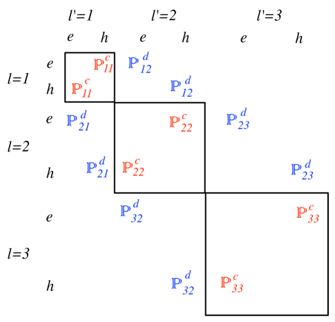
Figure S1: The structure of the force matrix $\mathbb{P}_{z}$

Now, let us focus on the $\mathbb{P}_{q}^{c}$. From (Farsund and Felderhof, 1996, Eqs. (7.19,7.20)), we have

$$\mathbb{P}_{q}^{c^{\prime}}(\ell mm^{\prime})=\frac{1}{\ell(\ell+1)}L_{q}(\ell mm^{\prime})$$ (S60)

Note that this term is not along the diagonal since it is the $e$-$h$ interaction. $\mathbb{P}_{q}^{c^{\prime}}$ has the same form for both $e-h$ and $h-e$ blocks. Again, there is a real operator for the force calculation, and therefore

$$\mathbb{P}_{q}^{c}=\frac{\mathbb{P}_{q}^{c^{\prime}}+(\mathbb{P}_{q}^{c^{\prime}})^{\dagger}}{2}.$$ (S61)

Finally, $\mathbb{P}_{q}=\mathbb{P}_{q}^{d}+\mathbb{P}_{q}^{c}$. Using the same $q\rightarrow i$ conversion as for the torque case,

$$\mathbb{P}_{z} =\mathbb{P}_{0}$$ (S62)

$$\mathbb{P}_{x} =\frac{\mathbb{P}_{+1}-\mathbb{P}_{-1}}{\sqrt{2}}$$ (S63)

$$\mathbb{P}_{y} =-i\frac{\mathbb{P}_{+1}+\mathbb{P}_{-1}}{\sqrt{2}}$$ (S64)

$\mathbb{P}_{z}$, for example, has the structure shown in Fig. S1.

IV Bounds on eigenvalues of $\mathbb{P}_{i}$ and $\mathbb{J}_{i}$ in the VSW basis

As we saw in Sec. III.1, the eigenvalues of the $\mathbb{J}_{i}$, for any $i$, are simply the diagonal entries of $\mathbb{J}_{z}$:

$$-\ell,-\ell+1,\ldots,\ell-1,\ell,$$

and thus the maximum eigenvalue is

$$\lambda_{\rm max}(\mathbb{J}_{i})=\ell_{\rm max}.$$ (S65)

For the force matrices $\mathbb{P}_{i}$, the off-diagonal components make it impossible (as far as we can tell) to solve for the eigenvalues analytically. The Gershgorin circle theorem Horn and Johnson (2013) can be used to get within about a factor of 1.5 of the largest eigenvalue, but it turns out that a simple physical argument yields a tighter bound.

Consider some set of incoming waves given by a set of coefficients $\bm{\mathbf{c}}_{\rm in}$. The momentum per time carried by those waves is given by $\frac{1}{c}\bm{\mathbf{c}}_{\rm in}^{\dagger}\mathbb{P}_{i}\bm{\mathbf{c}}_{\rm in}$. The maximum momentum that could be carried by those waves is given by the number of photons per unit time multiplied by $\hbar k$, i.e. the total momentum is less than or equal to the sum of $\hbar k=\hbar\omega/c$ for each photon. The number of photons per unit time is given by $\bm{\mathbf{c}}_{\rm in}^{\dagger}\bm{\mathbf{c}}_{\rm in}/\hbar\omega$, since $\bm{\mathbf{c}}_{\rm in}^{\dagger}\bm{\mathbf{c}}_{\rm in}$ is the incoming power. Following these arguments mathematically, we can write:

$$\frac{1}{c}\bm{\mathbf{c}}_{\rm in}^{\dagger}\mathbb{P}_{i}\bm{\mathbf{c}}_{\rm in} \leq\hbar k\frac{dN}{dt}$$

$$=\hbar k\frac{\bm{\mathbf{c}}_{\rm in}^{\dagger}\bm{\mathbf{c}}_{\rm in}}{\hbar\omega}$$

$$=\frac{1}{c}\bm{\mathbf{c}}_{\rm in}^{\dagger}\bm{\mathbf{c}}_{\rm in}.$$

We can rewrite the final expression without the speed of light,

$$\bm{\mathbf{c}}_{\rm in}^{\dagger}\mathbb{P}_{i}\bm{\mathbf{c}}_{\rm in}\leq\bm{\mathbf{c}}_{\rm in}^{\dagger}\bm{\mathbf{c}}_{\rm in},$$ (S66)

which applies for any $\bm{\mathbf{c}}_{\rm in}$ vector, implying that

$$\lambda_{\rm max}(\mathbb{P}_{i})\leq 1.$$ (S67)

Fig. S2 shows that the largest eigenvalue of $\mathbb{P}_{i}$ in a VSW basis converges to the bound as $\ell_{\rm max}\rightarrow\infty$. Note that the eigenvalue bound itself does not rely on any property of VSWs and must be true for any basis.

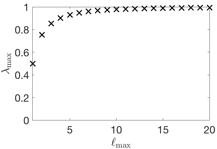
Figure S2: Largest eigenvalue of $\mathbb{P}_{i}$ as a function of $\ell_{\rm max}$, converging to the bound of 1.

V Plane-wave power and momentum in the VSW basis

In this section we derive the quantities $\bm{\mathbf{c}}_{\rm in}^{\dagger}\bm{\mathbf{c}}_{\rm in}$, $\bm{\mathbf{c}}_{\rm in}^{\dagger}\mathbb{P}_{i}\bm{\mathbf{c}}_{\rm in}$, and $\bm{\mathbf{c}}_{\rm in}^{\dagger}\mathbb{J}_{i}\bm{\mathbf{c}}_{\rm in}$ in the case that $\bm{\mathbf{c}}_{\rm in}$ represents the VSW coefficients for a plane wave propagating in the $z$ direction. We can start from the plane-wave expansions in Bohren and Huffman (1983) and convert to our VSW basis to find the incoming-wave coefficients. Plane waves have nonzero coefficients only for $m=\pm 1$; taking $m=1$ below, the coefficients for linear polarization are

$$\bm{\mathbf{c}}_{e\ell m}^{\rm Lin} =\frac{1}{2}\sqrt{\pi(2\ell-1)}i^{\ell-1}$$ (S68a)

$$\bm{\mathbf{c}}_{e\ell-m}^{\rm Lin} =-\frac{1}{2}\sqrt{\pi(2\ell-1)}i^{\ell-1}$$ (S68b)

$$\bm{\mathbf{c}}_{h\ell m}^{\rm Lin} =\frac{1}{2}\sqrt{\pi(2\ell+1)}i^{\ell-1}$$ (S68c)

$$\bm{\mathbf{c}}_{h\ell-m}^{\rm Lin} =\frac{1}{2}\sqrt{\pi(2\ell+1)}i^{\ell-1},$$ (S68d)

for right circular polarization they are

$$\bm{\mathbf{c}}_{e\ell m}^{\rm RCP} =\frac{1}{2}\sqrt{2\pi(2\ell-1)}i^{\ell-1}$$ (S69a)

$$\bm{\mathbf{c}}_{h\ell m}^{\rm RCP} =\frac{1}{2}\sqrt{2\pi(2\ell+1)}i^{\ell-1},$$ (S69b)

and for left circular polarization they are

$$\bm{\mathbf{c}}_{e\ell-m}^{\rm LCP} =-\frac{1}{2}\sqrt{2\pi(2\ell-1)}i^{\ell-1}$$ (S70a)

$$\bm{\mathbf{c}}_{h\ell-m}^{\rm LCP} =\frac{1}{2}\sqrt{2\pi(2\ell+1)}i^{\ell-1}.$$ (S70b)

The value of $\bm{\mathbf{c}}_{\rm in}^{\dagger}\bm{\mathbf{c}}_{\rm in}$ is the same for any polarization (since the power is not affected by polarization). It is simplest to compute the power for circular polarization, in which case it is the sum $\frac{1}{2}\sum_{\ell=1}^{\ell_{\rm max}}2\pi\left(2\ell+1\right)$. At this point we rescale our coefficients by the value $\frac{|\mathbf{E}_{0}|}{k\sqrt{2Z_{0}}}$, where $\mathbf{E}_{0}$ is the plane-wave amplitude, $k$ the wavenumber, and $Z_{0}$ the impedance of free space (to ultimately yield a power-normalized $\bm{\mathbf{c}}_{\rm in}^{\dagger}\bm{\mathbf{c}}_{\rm in}$). Then,

$$\bm{\mathbf{c}}_{\rm in}^{\dagger}\bm{\mathbf{c}}_{\rm in} =\frac{\pi}{k^{2}}\frac{|\mathbf{E}_{0}|^{2}}{2Z_{0}}\left(\ell_{\rm max}^{2}+2\ell_{\rm max}\right).$$ (S71)

All of the following quantities will ultimately be written in terms of $\bm{\mathbf{c}}_{\rm in}^{\dagger}\bm{\mathbf{c}}_{\rm in}$, so we drop the scale factor $|\mathbf{E}_{0}|/k\sqrt{2Z_{0}}$ hereafter.

Now we consider the momentum flowing in direction $i$. The momentum per time is given by $(\hat{\bm{\mathbf{z}}}\cdot\hat{\bm{\mathbf{i}}})\bm{\mathbf{c}}_{\rm in}^{\dagger}\mathbb{P}_{z}\bm{\mathbf{c}}_{\rm in}/c=\beta_{i}\bm{\mathbf{c}}_{\rm in}^{\dagger}\mathbb{P}_{z}\bm{\mathbf{c}}_{\rm in}/c$, since there is no $x$- or $y$-directed momentum. (It can be verified that $\bm{\mathbf{c}}_{\rm in}^{\dagger}\mathbb{P}_{x}\bm{\mathbf{c}}_{\rm in}=\bm{\mathbf{c}}_{\rm in}^{\dagger}\mathbb{P}_{y}\bm{\mathbf{c}}_{\rm in}=0$.) From Sec. III.2, we know that $\mathbb{P}_{z}=\mathbb{P}_{z}^{d}+\mathbb{P}_{z}^{c}$. We saw that

$$\mathbb{P}_{z}^{c}(\ell mm^{\prime})=\frac{1}{\ell(\ell+1)}L_{0}(\ell mm^{\prime})~{},$$

which means that

$$\bm{\mathbf{c}}_{\rm in}^{\dagger}\mathbb{P}_{z}^{c}\bm{\mathbf{c}}_{\rm in} =\sum_{\ell=1}^{\ell_{\rm max}}\frac{1}{\ell(\ell+1)}\overline{c_{\ell}}c_{\ell}$$

$$=\pi\sum_{\ell=1}^{\ell_{\rm max}}\frac{2\ell+1}{\ell(\ell+1)},$$ (S72)

where we used the fact that $\bm{\mathbf{c}}_{\rm in}$ has nonzero coefficients only for $m=1$, for which $L_{0}(\ell mm^{\prime})=\delta_{mm^{\prime}}$. From Eq. (S52), the $\mathbb{P}_{z}^{d}$ contribution is

$$\bm{\mathbf{c}}_{\rm in}^{\dagger}\mathbb{P}_{z}^{d}\bm{\mathbf{c}}_{\rm in} =\sum_{\ell=1}^{\ell_{\rm max}-1}\frac{1}{2}\left[(\ell^{2}+\ell-1)+\left(\ell+1\right)^{2}+\ell+1-1\right]$$

$$\cdot\sqrt{\frac{(\ell+2)\ell}{(2\ell+1)(2\ell+3)}}\cdot\sqrt{\frac{1}{\ell(\ell+1)}}\cdot\sqrt{\frac{1}{(\ell+1)(\ell+2)}}$$

$$\cdot\sqrt{2\pi(2\ell+1)}\cdot\sqrt{2\pi(2\ell+3)}$$

$$=\pi\sum_{\ell=1}^{\ell_{\rm max}-1}\frac{2\ell(\ell+2)}{(\ell+1)}$$ (S73)

The first line of the above equation is the summation of the $\{\ell,(\ell+1)\}$ and $\{(\ell+1),\ell\}$ interaction. For both interactions, $R_{q}(\ell m,\ell^{\prime}m^{\prime})$ is the same. We vary $\ell$ from $1$ to $\ell_{\rm max}-1$ since the interaction only comes into play when $\ell_{\rm max}\geq 2$. The first term of the second line includes $R_{q}(\ell m,\ell^{\prime}m^{\prime})$. The third line incorporates the values of $\bm{\mathbf{c}}_{\rm in}$ for channels $\ell$ and $\ell+1$. So the sum of the contributions from $\mathbb{P}_{z}^{c}$ and $\mathbb{P}_{z}^{d}$ is

$$\bm{\mathbf{c}}_{\rm in}^{\dagger}\mathbb{P}_{z}\bm{\mathbf{c}}_{\rm in} =\pi\sum_{\ell=1}^{\ell_{\rm max}-1}\frac{2\ell+1}{\ell(\ell+1)}+\pi\frac{2\ell_{\rm max}+1}{\ell_{\rm max}(\ell_{\rm max}+1)}+\pi\sum_{\ell=1}^{\ell_{\rm max}-1}\frac{2\ell(\ell+2)}{(\ell+1)}$$

$$=\pi\sum_{\ell=1}^{\ell_{\rm max}-1}\frac{2\ell(\ell+1)^{2}}{\ell(\ell+1)}+\pi\sum_{\ell=1}^{\ell_{\rm max}-1}\frac{1}{\ell(\ell+1)}+\pi\frac{2\ell_{\rm max}+1}{\ell_{\rm max}(\ell_{\rm max}+1)}$$

$$=\pi\sum_{\ell=1}^{\ell_{\rm max}-1}2(\ell+1)+\pi\cdot\frac{\ell_{\rm max}-1}{\ell_{\rm max}}+\pi\frac{2\ell_{\rm max}+1}{\ell_{\rm max}(\ell_{\rm max}+1)}$$

$$=\pi\left(\ell_{\rm max}^{2}+\ell_{\rm max}-2+\frac{\ell_{\rm max}-1}{\ell_{\rm max}}+\frac{2\ell_{\rm max}+1}{\ell_{\rm max}(\ell_{\rm max}+1)}\right)$$

$$=\pi(\ell_{\rm max}^{2}+2\ell_{\rm max})\frac{\ell_{\rm max}}{\ell_{\rm max}+1}$$

$$=\frac{\ell_{\rm max}}{\ell_{\rm max}+1}\bm{\mathbf{c}}_{\rm in}^{\dagger}\bm{\mathbf{c}}_{\rm in}.$$ (S74)

And thus the momentum flow per time in direction $i$, denoted $\mathcal{P}_{\textrm{in},i}$ in the main text, is

$$\mathcal{P}_{\textrm{in},i}=\frac{\beta_{i}}{c}\frac{\ell_{\rm max}}{\ell_{\rm max}+1}\bm{\mathbf{c}}_{\rm in}^{\dagger}\bm{\mathbf{c}}_{\rm in}.$$ (S75)

Finally, for the angular momentum, we separately consider the RCP and LCP waves, and at the end show that the total angular momentum is proportional to the degree of right circular polarization. Again, one can show for any $\bm{\mathbf{c}}_{\rm in}$ that $\bm{\mathbf{c}}_{\rm in}^{\dagger}\mathbb{J}_{x}\bm{\mathbf{c}}_{\rm in}=\bm{\mathbf{c}}_{\rm in}^{\dagger}\mathbb{J}_{y}\bm{\mathbf{c}}_{\rm in}=0$, such that the angular momentum in direction $i$ is determined by the $z$-directed fraction,

$$\bm{\mathbf{c}}_{\rm in}^{\dagger}\mathbb{J}_{i}\bm{\mathbf{c}}_{\rm in}=\beta_{i}\bm{\mathbf{c}}_{\rm in}^{\dagger}\mathbb{J}_{z}\bm{\mathbf{c}}_{\rm in}.$$ (S76)

For an RCP plane wave, the coefficients of $\bm{\mathbf{c}}_{\rm in}$ are nonzero only for $m=1$, for which the diagonal entries of $\mathbb{J}_{z}$ are $1$, such that $\bm{\mathbf{c}}_{\rm in}^{\dagger}\mathbb{J}_{z}\bm{\mathbf{c}}_{\rm in}=\bm{\mathbf{c}}_{\rm in}^{\dagger}\bm{\mathbf{c}}_{\rm in}$. Conversely, for an LCP plane wave the coefficients of $\bm{\mathbf{c}}_{\rm in}$ are nonzero only for $m=-1$, for which the diagonal entries of $\mathbb{J}_{z}$ are $-1$, such that $\bm{\mathbf{c}}_{\rm in}^{\dagger}\mathbb{J}_{z}\bm{\mathbf{c}}_{\rm in}=-\bm{\mathbf{c}}_{\rm in}^{\dagger}\bm{\mathbf{c}}_{\rm in}$, the negative of the RCP case. Thus is we define $\gamma_{i}$ as the degree of right circular polarization of any incoming wave, the angular momentum per unit time is

$$\mathcal{J}_{\textrm{in},i}=\frac{\beta_{i}\gamma_{i}}{\omega}\bm{\mathbf{c}}_{\rm in}^{\dagger}\bm{\mathbf{c}}_{\rm in}.$$ (S77)

VI Force bound when $\ell_{\rm max}=1$

In the main text, we derived force and torque bounds in a VSW basis for plane-wave incidence for any $\ell_{\rm max}$, using the eigenvalue bound $\lambda_{\rm max}(\mathbb{P}_{i})=1$. Here, we consider the case $\ell_{\rm max}=1$. In this case, analysis of the matrices in Sec. III.2 shows that $\lambda_{\rm max}(\mathbb{P}_{z})=1/2$. Carrying this factor of 1/2 through the bound derivation, one finds that the force in the $i$ direction normalized by the incident-wave intensity is bounded above by

$$\frac{F_{i}}{I_{\rm inc}} \leq\frac{3\lambda^{2}}{4\pi c},$$ (S78)

about a factor of 1/3 tighter than the bound in the main text, for this special case.

VII Helix: structural details

The line running along the center of a helix wrapping around the $z$ axis has a simple parametrization:

$$\bm{\mathbf{r}}(t)=(R\cos(t),R\sin(t),ht),$$ (S79)

where $R$ controls the radius of that center line as it wraps, and $h$ scales the rate at which the height along $z$ changes. The parameter $t$ controls how many rotations of the helix occur, e.g. $[0,4\pi]$ means two circles. For a three-dimensional helical structure, we need two unit vectors at each point along the center line, to create the circular surface slice of the helix. Starting with the tangent vector (by differentiation),

$$\bm{\mathbf{t}}(t)=(-R\sin(t),R\cos(t),h),$$ (S80)

one can get the local normal vector as

$$\bm{\mathbf{n}}(t)=(-\cos(t),-\sin(t),0).$$ (S81)

The second local basis vector is the “binormal,”

$$\bm{\mathbf{b}}(t)=\bm{\mathbf{t}}\times\bm{\mathbf{n}}=\frac{1}{\sqrt{R^{2}+h^{2}}}(h\sin(t),-h\cos(t),R).$$ (S82)

To create the 3D helix, we thus use a vector $\bm{\mathbf{S}}$ that is the sum of $\bm{\mathbf{r}}(t)$ with two new parameters and the two basis vectors. We use a parameter $u$ which ranges from 0 to $2\pi$, to create the circular surfaces around the helical line, and a second parameter $a$ that represents the radius of the circle that wraps around the center line (not the radius of the circle formed by the center line itself, which is $R$).

$$\bm{\mathbf{S}}(u,t)=\bm{\mathbf{r}}(t)+a\bm{\mathbf{n}}(t)\cos(u)+a\bm{\mathbf{b}}(t)\sin(u).$$ (S83)

For the structure simulated in the main text, we used the values $R=0.9$, $a=0.45$, and $h=0.3$.

VIII Cross-section bounds rederived

In this final section we derive VSW bounds on scattering, absorption, and extinction cross-sections for plane-wave illumination, and verify that the resulting bounds agree with previous results from the literature Hamam et al. (2007); Kwon and Pozar (2009); Ruan and Fan (2011); Liberal et al. (2014); Hugonin et al. (2015). To examine scattered power and extinction, we will need to connect the incoming-field/outgoing-field separation to the common incident-field/scattered-field separation. For VSWs, it is generally true for any incident field that half of the field must be incoming and the other half must be outgoing (to have a continuous field at the origin, where incoming/outgoing fields have singularities) Doicu et al. (2006). The scattered field must be purely outgoing. Thus, the relationship between the in/out coefficients $\bm{\mathbf{c}}_{\rm in}$ and $\bm{\mathbf{c}}_{\rm out}$, and the inc/scat coefficients $\bm{\mathbf{c}}_{\rm inc}$ and $\bm{\mathbf{c}}_{\rm scat}$ is given by Eqs. (S20,S21).

We start with absorption, the bound for which is particularly simple. Absorption is given by $\bm{\mathbf{c}}_{\rm in}^{\dagger}\bm{\mathbf{c}}_{\rm in}-\bm{\mathbf{c}}_{\rm out}^{\dagger}\bm{\mathbf{c}}_{\rm out}$, and thus maximum absorption satisfies

$$\underset{\bm{\mathbf{c}}_{\rm out}}{\text{maximize}} \bm{\mathbf{c}}_{\rm in}^{\dagger}\bm{\mathbf{c}}_{\rm in}-\bm{\mathbf{c}}_{\rm out}^{\dagger}\bm{\mathbf{c}}_{\rm out}$$ (S84)

subject to $$\bm{\mathbf{c}}_{\rm out}^{\dagger}\bm{\mathbf{c}}_{\rm out}\leq\bm{\mathbf{c}}_{\rm in}^{\dagger}\bm{\mathbf{c}}_{\rm in}.$$

Maximum absorption occurs when $\bm{\mathbf{c}}_{\rm out}^{\dagger}\bm{\mathbf{c}}_{\rm out}=0$ (all power is incoming and absorbed), such that

$$P_{\rm abs}^{\rm(max)}=\bm{\mathbf{c}}_{\rm in}^{\dagger}\bm{\mathbf{c}}_{\rm in}=\frac{\pi|\mathbf{E}_{0}|^{2}}{2k^{2}Z_{0}}\left(\ell_{\rm max}^{2}+2\ell_{\rm max}\right)$$ (S85)

The absorption cross-section is the absorbed power divided by the incident intensity, $I_{\rm inc}=|\mathbf{E}_{0}|^{2}/2Z_{0}$. Then the maximum absorption cross-section is

$$\sigma_{\rm abs}^{\rm(max)}=\frac{\pi}{k^{2}}\left(\ell_{\rm max}^{2}+2\ell_{\rm max}\right)=\frac{\lambda^{2}}{4\pi}\left(\ell_{\rm max}^{2}+2\ell_{\rm max}\right).$$ (S86)

Scattered power is the outgoing power in the scattered fields, and hence is given by $\bm{\mathbf{c}}_{\rm scat}^{\dagger}\bm{\mathbf{c}}_{\rm scat}$. By Eqs. (S20,S21), $\bm{\mathbf{c}}_{\rm scat}=\bm{\mathbf{c}}_{\rm out}-\bm{\mathbf{c}}_{\rm in}$, such that maximum scattered power is the solution to the optimization problem

$$\underset{\bm{\mathbf{c}}_{\rm out}}{\text{maximize}} \left(\bm{\mathbf{c}}_{\rm out}-\bm{\mathbf{c}}_{\rm in}\right)^{\dagger}\left(\bm{\mathbf{c}}_{\rm out}-\bm{\mathbf{c}}_{\rm in}\right)$$ (S87)

subject to $$\bm{\mathbf{c}}_{\rm out}^{\dagger}\bm{\mathbf{c}}_{\rm out}\leq\bm{\mathbf{c}}_{\rm in}^{\dagger}\bm{\mathbf{c}}_{\rm in}.$$

Lagrangian multipliers confirm the intuition that the optimal $\bm{\mathbf{c}}_{\rm out}$ is the negative of $\bm{\mathbf{c}}_{\rm in}$: $\bm{\mathbf{c}}_{\rm out}=-\bm{\mathbf{c}}_{\rm in}$. Then the scattered power will be $4\bm{\mathbf{c}}_{\rm in}^{\dagger}\bm{\mathbf{c}}_{\rm in}$, i.e. 4 times the maximum absorbed power, and the maximum scattering cross-section is

$$\sigma_{\rm scat}^{\rm(max)}=\frac{4\pi}{k^{2}}\left(\ell_{\rm max}^{2}+2\ell_{\rm max}\right)=\frac{\lambda^{2}}{\pi}\left(\ell_{\rm max}^{2}+2\ell_{\rm max}\right).$$ (S88)

Extinction is the sum of the absorbed and scattered powers, and thus equals $2\operatorname{Re}\bm{\mathbf{c}}_{\rm in}^{\dagger}\left(\bm{\mathbf{c}}_{\rm in}-\bm{\mathbf{c}}_{\rm out}\right)$ (which equals the more intuitive expression $\operatorname{Re}\bm{\mathbf{c}}_{\rm inc}^{\dagger}\bm{\mathbf{c}}_{\rm scat}$). Then the maximum extinction satisfies

$$\underset{\bm{\mathbf{c}}_{\rm out}}{\text{maximize}} 2\operatorname{Re}\bm{\mathbf{c}}_{\rm in}^{\dagger}\left(\bm{\mathbf{c}}_{\rm in}-\bm{\mathbf{c}}_{\rm out}\right)$$ (S89)

subject to $$\bm{\mathbf{c}}_{\rm out}^{\dagger}\bm{\mathbf{c}}_{\rm out}\leq\bm{\mathbf{c}}_{\rm in}^{\dagger}\bm{\mathbf{c}}_{\rm in}.$$

The maximum is achieved at the maximum-scattering condition, $\bm{\mathbf{c}}_{\rm out}=-\bm{\mathbf{c}}_{\rm in}$, meaning the extinction cross-section has the same upper bound as the scattering cross-section:

$$\sigma_{\rm ext}^{\rm(max)}=\frac{4\pi}{k^{2}}\left(\ell_{\rm max}^{2}+2\ell_{\rm max}\right)=\frac{\lambda^{2}}{\pi}\left(\ell_{\rm max}^{2}+2\ell_{\rm max}\right).$$ (S90)

References

- Suh et al. (2004) Wonjoo Suh, Zheng Wang, and Shanhui Fan, “Temporal coupled-mode theory and the presence of non-orthogonal modes in lossless multimode cavities,” IEEE J. Quantum Electron. 40, 1511–1518 (2004).
- Tsang et al. (2000) Leung Tsang, Jin Au Kong, and Kung-Hau Ding, Scattering of Electromagnetic Waves: Theories and Applications (John Wiley & Sons, Inc., New York, USA, 2000).
- Bohren and Huffman (1983) Craig F. Bohren and Donald R. Huffman, Absorption and Scattering of Light by Small Particles (John Wiley & Sons, New York, NY, 1983).
- Farsund and Felderhof (1996) Ø. Farsund and B. U. Felderhof, “Force, torque, and absorbed energy for a body of arbitrary shape and constitution in an electromagnetic radiation field,” Physica A 227, 108–130 (1996).
- Horn and Johnson (2013) Roger A. Horn and Charles R. Johnson, Matrix Analysis, 2nd ed. (Cambridge University Press, New York, NY, 2013).
- Hamam et al. (2007) Rafif E. Hamam, Aristeidis Karalis, J. D. Joannopoulos, and Marin Soljačić, “Coupled-mode theory for general free-space resonant scattering of waves,” Phys. Rev. A 75, 053801 (2007).
- Kwon and Pozar (2009) Do-Hoon Kwon and David M. Pozar, “Optimal Characteristics of an Arbitrary Receive Antenna,” IEEE Trans. Antennas Propag. 57, 3720–3727 (2009).
- Ruan and Fan (2011) Zhichao Ruan and Shanhui Fan, “Design of subwavelength superscattering nanospheres,” Appl. Phys. Lett. 98, 043101 (2011).
- Liberal et al. (2014) Inigo Liberal, Younes Ra’di, Ramon Gonzalo, Inigo Ederra, Sergei A. Tretyakov, and Richard W. Ziolkowski, “Least Upper Bounds of the Powers Extracted and Scattered by Bi-anisotropic Particles,” IEEE Trans. Antennas Propag. 62, 4726–4735 (2014).
- Hugonin et al. (2015) Jean-Paul Hugonin, Mondher Besbes, and Philippe Ben-Abdallah, “Fundamental limits for light absorption and scattering induced by cooperative electromagnetic interactions,” Phys. Rev. B 91, 180202 (2015).
- Doicu et al. (2006) Adrian Doicu, Thomas Wriedt, and Yuri A Eremin, Light scattering by systems of particles: null-field method with discrete sources: theory and programs, Vol. 124 (Springer, 2006).