A new twist on heterotic string compactifications

Bernardo Fraiman${}^{{\dagger}\,*}$, Mariana Graña^# and Carmen A. Nuñez${}^{{\dagger}\,*}$
^† Instituto de Astronomía y Física del Espacio (IAFE-CONICET-UBA)
Ciudad Universitaria, Pabellón IAFE, 1428 Buenos Aires, Argentina
^∗ Departamento de Física, FCEyN, Universidad de Buenos Aires (UBA)
^# Institut de Physique Théorique, CEA/ Saclay
91191 Gif-sur-Yvette Cedex, France

E-mail:  bfraiman@iafe.uba.ar,  mariana.grana@ipht.fr,  carmen@iafe.uba.ar

Abstract: A rich pattern of gauge symmetries is found in the moduli space of heterotic string toroidal compactifications, at fixed points of the T-duality transformations. We analyze this pattern for generic tori, and scrutinize in full detail compactifications on a circle, where we find all the maximal gauge symmetry groups and the points where they arise. We present figures of two-dimensional slices of the 17-dimensional moduli space of Wilson lines and circle radii, showing the rich pattern of points and curves of symmetry enhancement. We then study the target space realization of the duality symmetry. Although the global continuous duality symmetries of dimensionally reduced heterotic supergravity are completely broken by the structure constants of the maximally enhanced gauge groups, the low energy effective action can be written in a manifestly duality covariant form using heterotic double field theory. As a byproduct, we show that a unique deformation of the generalized diffeomorphisms accounts for both $SO(32)$ and $E_{8}\times E_{8}$ heterotic effective field theories, which can thus be considered two different backgrounds of the same double field theory even before compactification. Finally we discuss the spontaneous gauge symmetry breaking and Higgs mechanism that occurs when slightly perturbing the background fields, both from the string and the field theory perspectives.

1 Introduction

The distinct backgrounds of heterotic string theory on a $k$ dimensional torus with constant metric, antisymmetric tensor field and Wilson lines are characterized by the points of the $\frac{O(k,k+16;\mathbb{R})}{O(k;\mathbb{R})\times O(k+16;\mathbb{R})\times O(k,k+16;\mathbb{Z})}$ coset manifold, where $O(k,k+16;\mathbb{Z})$ is the T-duality group [1, 2]. At self-dual points of this manifold, some massive modes become massless and the $U(1)^{2k+16}$ gauge symmetry becomes non-abelian. In particular, for zero Wilson lines, the massless fields give rise to $SO(32)\times U(1)^{2k}$ or $E_{8}\times E_{8}\times U(1)^{2k}$ at generic values of the metric and B-field. By introducing Wilson lines, not only is it possible to totally or partially break the non-abelian gauge symmetry of the uncompactified theory, but it is also possible to enhance these groups. The construction of [2] further allowed to continuously interpolate between the $SO(32)$ and $E_{8}\times E_{8}$ heterotic theories after compactification [3], and even suggested that these superstrings are two different vacuum states in the same theory before compactification.

Enhancement of the gauge symmetry occurs at fixed points of the T-duality transformations [4]. Massless fields become massive at the neighborhood of such points and the T-duality group mixes massless modes with massive ones [5]. Moreover, by identifying different string backgrounds that provide identical theories, T-duality gives rise to stringy features that are rather surprising from the viewpoint of particle field theories. Nevertheless, some of these ingredients have a correspondence in toroidal compactifications of heterotic supergravity. In particular, although the field theoretical reduction of heterotic supergravity cannot describe the non-abelian fields that give rise to maximally enhanced gauge symmetry, being a gauged supergravity, the reduced theory is completely determined by the gauge group, which can be chosen to be one of maximal enhancement. Likewise, the global symmetries of heterotic supergravities are linked to T-duality. While the theory with the full set of $SO(32)$ or $E_{8}\times E_{8}$ gauge fields has a global continuous $O(k,k;\mathbb{R})$ symmetry, when introducing Wilson lines, the symmetry enlarges to $O(k,k+16;{\mathbb{R}})$ [6, 7, 8], which is related to the discrete T-duality symmetry of the parent string theory.

The global duality symmetries are not manifest in heterotic supergravity. To manifestly display these symmetries, as well as to account for the maximally enhanced gauge groups in a field theoretical setting, one appeals to the double field theory/generalized geometric reformulation of the string effective actions [9, 10] (for reviews and more references see [11]). Specifically, these frameworks not only describe the enhancement of gauge symmetry [12]-[15], but also give a geometric description of the non-geometric backgrounds that are obtained from T-duality [16] and provide a gauge principle that requires and fixes the $\alpha^{\prime}$-corrections of the string effective actions [17]. Dependence of the fields on double internal coordinates and an extension of the tangent space are some of the elements that allow to go beyond the standard dimensional reductions of supergravity.

Motivated by deepening our understanding of heterotic string toroidal compactifications, in section 2 we review the main features of heterotic string propagation on a $(10-k)$-dimensional Minkowski space-time times an internal $k$-torus with constant background metric, antisymmetric tensor field and Wilson lines, and recall their $O(k,k+16)$ covariant formulation. We focus on the phenomenon of symmetry enhancement arising at special points in moduli space.

In section 3, we concentrate on the simplest case, namely circle compactifications ($k=1$). We first find all the possible maximal enhancement groups, and the point in the fundamental region of moduli space where they arise, using the generalized Dynkin diagram of the lattice $\Gamma^{1,17}$ [18, 21]. To explore the whole moduli space, we split the discussion into the situations in which the Wilson line $A$ preserves the $E_{8}\times E_{8}$ or $SO(32)$ gauge symmetry, and those where it breaks it. In the former case, the circle direction can give a further enhancement of symmetry to $E_{8}\times E_{8}\times SU(2)$ at radius $R=1$, and either to $SO(32)\times SU(2)$ at $R=1$ or to $SO(34)$ at $R=\frac{1}{\sqrt{2}}$. When the Wilson line breaks the $E_{8}\times E_{8}$ or $SO(32)$ gauge symmetry, the pattern of gauge symmetries is very interesting. Not only is it possible to restore the original $E_{8}\times E_{8}$ or $SO(32)$ gauge symmetry for specific values of $R$ and $A$, but also larger groups of rank 17 can be obtained. We explicitly work out enhancements of the $SO(32)$ theory to $SO(34)$ at $R^{2}=\tfrac{1}{2}$; $SU(18)$ at $R^{2}=\tfrac{1}{4}$; $E_{p+1}\times SO(32-2p)$ at $R^{2}=1-\tfrac{p}{8}$; $E_{p+1}\times SU(16-p)$ at $R^{2}=1-\tfrac{8}{16-p}$, and in the $E_{8}\times E_{8}$ to $SO(34)$ at $R^{2}=\tfrac{1}{18}$; $SU(18)$ at $R^{2}=\tfrac{1}{9}$; $SO(18)\times E_{8}$ at $R^{2}=\frac{1}{2}$; $SU(2)\times E_{8}\times E_{8}$ at $R^{2}=\tfrac{1}{4}$. We depict slices of the moduli space for different values of $R$ and Wilson lines in several figures, which clarify the analysis and neatly exhibit the curves and points with special properties.

Examining the action of T-duality, we can see that all points in moduli space where there is maximal symmetry enhancement, namely enhancement to groups that do not have $U(1)$ factors, are fixed points of T-duality, or more general $O(1,17,{\mathbb{Z}})$ dualities that involve some exchange of momentum and winding number on the circle. In the simplest cases, such as those listed above, the enhanced symmetry arises at the self-dual radius given by $R^{2}_{sd}=1-\frac{1}{2}|A|^{2}$. We explore the action of T-duality and its fixed points in section 3.4. One can have other points of symmetry enhancement, which are fixed points of duality symmetries that involve shifts of Wilson lines on top of the exchange of momentum and winding. This is studied in detail in section 3.5, where we obtain the most general duality symmetries that change the sign of the right-moving momenta and rotate the left-moving momenta, leaving the circle direction invariant. Concentrating on the case where the Wilson lines have only one non-zero component, we find a rich pattern of fixed points that correspond to $SU(2)\times SO(32)$ or $SU(2)\times E_{8}\times E_{8}$ enhanced gauge symmetry, arising at $R_{\rm sd}^{-1}=C$, with $C$ an integer number with prime divisors congruent to 1 or 3 (mod 8), and $SO(34)$ or $SO(18)\times E_{8}$ at $R_{\rm sd}^{-1}=\sqrt{2}\,C$ with $C$ a Pythagorean prime number or a product of them.

We then turn to the target space realization of the theory. In section 4, we construct the low energy effective actions of (toroidally compactified) heterotic strings from the three and four point functions of string states. We first consider only the massless states and compare the effective action obtained from the string amplitudes with the dimensional reduction of heterotic supergravity performed in [8]. As expected, we get a gauged supergravity which only differs from the effective action of [8] in the cases of maximal enhancement, in which all the (left-moving) $U(1)^{k}$ Kaluza-Klein (KK) gauge fields of the compactification become part of the Cartan subgroup of the enhanced gauge symmetry.

The higher dimensional origin of the low energy theory with maximally enhanced gauge symmetry cannot be found in supergravity, and one has to refer to DFT. Although the structure constants of the gauge group completely break the global duality symmetry of dimensionally reduced supergravity, the action can still be written in terms of $O(k,N)$ multiplets, with $N$ the dimension of the gauge group. We show in section 5 that the low energy effective action of the toroidally compactified heterotic string at self-dual points of the moduli space can be reproduced through a generalized Scherk-Schwarz reduction of heterotic DFT. Furthermore, extending the construction of [13], we find the generalized vielbein that reproduces the structure constants of the enhanced gauge groups through a deformation of the generalized diffeomorphisms. An important output of the construction is that a unique deformation is required for the $SO(32)$ and $E_{8}\times E_{8}$ groups, and hence the $SO(32)$ and $E_{8}\times E_{8}$ theories can be considered two different solutions of the same heterotic DFT, even before compactification.

When perturbing the background fields away from the enhancement points, some massless string states become massive. The vertex operators of the massive vector bosons develop a cubic pole in their OPE with the energy-momentum tensor, and it is necessary to combine them with the vertex operators of the massive scalars in order to cancel the anomaly. This fact had been already noticed in [12], but unlike the case of the bosonic string, in the heterotic string all the massive scalars are “eaten” by the massive vectors. We compute the three point functions involving massless and slightly massive states and construct the corresponding effective massive gauge theory coupled to gravity. Comparing the string theory results with the spontaneous gauge symmetry breaking and Higgs mechanism in DFT, we see that the masses acquired by the sligthly massive string states fully agree with those of the DFT fields, provided there is a specific relation between the vacuum expectation value of the scalars along the Cartan directions of the gauge group and the deviation of the metric, B-field and Wilson lines from the point of enhancement.

We have included seven appendices. Appendix A collects some known facts about lattices that are used in the main body of the paper. Details of the procedures leading to find the maximal enhancement points from Dynkin diagrams, to construct the curves of enhancement, more slices of the moduli space and the fixed points of the duality transformations are contained in Appendices B, C, D and E, respectively. The three and four point amplitudes of the massless and slightly massive string states are reviewed in Appendix F. Finally we count the number of non-vanishing structure constants of $SO(32)$ and $E_{8}\times E_{8}$ in Appendix G.

2 Toroidal compactification of the heterotic string

In this section we recall the main features of heterotic string compactifications on $T^{k}$. We first discuss the generic $k$ case and then we concentrate on the $k=1$ example. For a more complete review see [5].

2.1 Compactifications on $T^{k}$

Consider the heterotic string propagating on a background manifold that is a product of a $d=10-k$ dimensional flat space-time times an internal torus $T^{k}$ with constant background metric $G=e^{t}e\ \left(\Rightarrow G_{mn}=e^{a}{}_{m}\delta_{ab}e^{b}{}_{n}\right.$), antisymmetric two-form field $B_{mn}$ and $U(1)^{16}$ gauge field $A_{m}^{A}$, where $m,n,a,b=1,...,k$ and $A=1,\dots,16$. For simplicity we take the background dilaton to be zero. The set of vectors $e_{m}$ define a basis in the compactification lattice $\Lambda^{k}$ such that the internal part of the target space is the $k$-dimensional torus $T^{k}=\mathbb{R}^{k}/\pi\Lambda^{k}$. The vectors $\hat{e}_{a}$ constitute the canonical basis for the dual lattice $\Lambda^{k*}$, i.e. $\hat{e}_{a}{}^{m}e^{a}{}_{n}=\delta^{m}{}_{n}$, and thus they obey $\hat{e}^{t}\hat{e}=G^{-1}\ \left(\Rightarrow\hat{e}_{a}{}^{m}\delta^{ab}\hat{e}_{b}{}^{n}=G^{mn}\right)$.

The contribution from the internal sector to the world-sheet action (we consider only the bosonic sector here) is

$$S = \frac{1}{4\pi}\int_{M}d\tau d\sigma\left(\delta^{\alpha\beta}G_{mn}-i\epsilon^{\alpha\beta}B_{mn}\right)\partial_{\alpha}Y^{m}\partial_{\beta}Y^{n}$$ (2.1)

$$+\frac{1}{8\pi}\int_{M}d\tau d\sigma\left(\delta^{\alpha\beta}\partial_{\alpha}Y^{A}\partial_{\beta}Y^{A}-2i\epsilon^{\alpha\beta}A_{m}^{A}\partial_{\alpha}Y^{m}\partial_{\beta}Y^{A}\right)\,,$$

where we take $\alpha^{\prime}=1$, $Y^{A}$ are chiral bosons and the currents $\partial Y^{A}$ form a maximal commuting set of the $SO(32)$ or $E_{8}\times E_{8}$ current algebra. The world-sheet metric has been gauge fixed to $\delta^{\alpha\beta}$ ($\alpha,\beta=\tau,\sigma$) and $\epsilon^{01}=1$. The internal string coordinate fields satisfy

$$Y^{m}(\tau,\sigma+2\pi)\simeq Y^{m}(\tau,\sigma)+2\pi w^{m}\ ,$$ (2.2)

where $w^{m}\in\mathbb{Z}$ are the winding numbers. It is convenient to define holomorphic $Y^{m}_{L}(z)$ and antiholomorphic $Y^{m}_{R}(\bar{z})$ fields as

$$Y^{m}(z,\bar{z})=\left(\frac{1}{2}\right)^{1/2}\left[Y^{m}_{L}(z)+Y^{m}_{R}(\bar{z})\right]\ ,\quad z=\exp(\tau+i\sigma)\ ,\ \bar{z}=\exp(\tau-i\sigma)\ ,$$ (2.3)

with Laurent expansion

$$Y^{m}_{L}(z) = y_{L}^{m}-ip^{m}_{L}\,lnz+\cdots,\qquad Y^{A}_{L}(z)=y_{L}^{A}-ip^{A}\,lnz+\cdots,$$ (2.4)

$$Y^{m}_{R}(\bar{z}) = y_{R}^{m}-ip^{m}_{R}\,ln\bar{z}+\cdots,$$ (2.5)

the dots standing for the oscillators contribution. Then the periodicity condition is

$$Y^{m}(\tau,\sigma+2\pi)-Y^{m}(\tau,\sigma)=2\pi\left(\frac{1}{2}\right)^{1/2}(p^{m}_{L}-p_{R}^{m})=2\pi w^{m}\ .$$ (2.6)

The canonical momentum has components

$$\Pi_{m} = i\frac{\delta S}{\delta\partial_{\tau}Y^{m}}=\frac{1}{2\pi}\left[iG_{mn}\partial_{\tau}Y^{n}+B_{mn}\partial_{\sigma}Y^{n}+\frac{1}{2}A_{m}^{A}\partial_{\sigma}Y^{A}\right]\,,$$

$$= \frac{1}{2\pi}\left(\frac{1}{2}\right)^{1/2}\left[G_{mn}(p_{L}^{n}+p_{R}^{n})+B_{mn}(p_{L}^{n}-p_{R}^{n})\right]+\frac{1}{4\pi}A_{m}^{A}p^{A}$$

$$\Pi^{A} = i\frac{\delta S}{\delta\partial_{\tau}Y^{A}}=\frac{1}{4\pi}\left(i\partial_{\tau}Y^{A}-A_{m}^{A}\partial_{\sigma}Y^{m}\right)=\frac{1}{2\pi}\left[p^{A}-\left(\frac{1}{2}\right)^{1/2}A_{m}^{A}(p_{L}^{m}-p_{R}^{m})\right]\,.$$

The chirality constraint on $Y^{A}$ and the condition of vanishing Dirac brackets between momentum components require the redefinitions $\Pi_{A}\rightarrow\tilde{\Pi}_{A}=2\Pi_{A}$ and $\Pi_{m}\rightarrow\tilde{\Pi}_{m}=\Pi_{m}+\frac{1}{2}A_{m}^{A}\tilde{\Pi}_{A}$. Integrating over $\sigma$, we get the center of mass momenta

$$\pi_{m} = \int d\sigma\tilde{\Pi}_{m}=2\pi\left(\Pi_{m}+\frac{1}{2}A_{m}^{A}\tilde{\Pi}_{A}\right)={n_{m}}\in{\mathbb{Z}}\,,$$ (2.7a)

$$\pi^{A} = \int d\sigma\tilde{\Pi}^{A}=p^{A}-A_{m}^{A}w^{m}\,,$$ (2.7b)

where we used univaluedness of the wave function in the first line. Modular invariance requires $\pi^{A}\in\Gamma_{16}$ or $\Gamma_{8}\times\Gamma_{8}$, corresponding to the $SO(32)$ or $E_{8}\times E_{8}$ heterotic theory, respectively. In Appendix A we give all the relevant explanations and details about these lattices.

From these equations we get

$$p_{Ra} = \left(\frac{1}{2}\right)^{1/2}\hat{e}_{a}{}^{m}\left[{n_{m}}-(G_{mn}+B_{mn})w^{n}-\pi^{A}A_{m}^{A}-\frac{1}{2}A_{n}^{A}A_{m}^{A}w^{n}\right]\,,$$ (2.8a)

$$p_{La} = \left(\frac{1}{2}\right)^{1/2}\hat{e}_{a}{}^{m}\left[{n_{m}}+(G_{mn}-B_{mn})w^{n}-\pi^{A}A_{m}^{A}-\frac{1}{2}A_{n}^{A}A_{m}^{A}w^{n}\right],$$ (2.8b)

$$p^{A} = \pi^{A}+w^{m}A^{A}_{m}\,.$$ (2.8c)

The momentum $\bf{p}=(\bf{p_{R},p_{L}})$, with ${\bf{p_{R}}}=p_{Ra},\ {\bf{p_{L}}}=(p_{La},p^{A})$, transforms as a vector under $O(k,k+16;\mathbb{R})$. It expands the $2k+16$-dimensional momentum lattice $\Gamma^{(k,k+16)}\subset{\mathbb{R}}^{2k+16}$, satisfying

$${\bf p}\cdot{\bf p}={\bf p_{L}}^{2}-{\bf p_{R}}^{2}=2w^{m}n_{m}+\pi^{A}\pi^{A}\in 2\mathbb{Z}\,,$$ (2.9)

because $\pi^{A}$ is on an even lattice, and therefore ${\bf p}$ forms an even $(k,k+16)$ Lorentzian lattice. In addition, self-duality $\Gamma^{(k,k+16)}=\Gamma^{(k,k+16)*}$ follows from modular invariance [1, 25]. Note that $\bf{p_{L},p_{R}}$ depend on $2k+16$ integer parameters $n_{m},w^{m}$ and $\pi^{A}$, and on the background fields $G$, $B$ and $A$.

The space of inequivalent lattices and inequivalent backgrounds reduces to

$$\frac{O(k,k+16;\mathbb{R})}{O(k+16;\mathbb{R})\times O(k;\mathbb{R})\times O(k,k+16;\mathbb{Z})}\,,$$ (2.10)

where $O(k,k+16;\mathbb{Z})$ is the T-duality group (we give more details about it in the next section).

The mass of the states and the level matching condition are respectively given by

$$m^{2}={\bf p_{L}}^{2}+{\bf p_{R}}^{2}+2\left({\cal N}+\overline{\cal N}-\left\{\begin{matrix}1&{\rm R\ sector}\\ \frac{3}{2}&{\rm NS\ sector}\end{matrix}\right.\right),$$ (2.11a)

$$0={\bf p_{L}}^{2}-{\bf p_{R}}^{2}+2\left({\cal N}-\overline{\cal N}-\left\{\begin{matrix}1&{\rm R\ sector}\\ \frac{1}{2}&{\rm NS\ sector}\end{matrix}\right.\right)\,.$$ (2.11b)

2.2 $O(k,k+16)$ covariant formulation

The $O(k,k+16)$ invariant metric $\eta$ is

$$\eta_{MN}=\begin{pmatrix}0&1_{k\times k}&0\\ 1_{k\times k}&0&0\\ 0&0&\kappa_{IJ}\end{pmatrix}\ ,\qquad$$ (2.12)

where $\kappa$ is the Killing metric for the Cartan subgroup of $SO(32)$ or $E_{8}\times E_{8}$, and the “generalized metric” of the $k$-dimensional torus, given by the $(2k+16)\times(2k+16)$ scalar matrix, is

$${\cal M}_{MN}=\begin{pmatrix}G_{mn}+C_{lm}G^{lk}C_{kn}+A_{m}{}^{I}A_{nI}&-G^{nk}C_{km}&C_{km}G^{kl}A_{lJ}+A_{mJ}\\ -G^{mk}C_{kn}&G^{mn}&-G^{mk}A_{kJ}\\ C_{kn}G^{kl}A_{lI}+A_{nI}&-G^{nk}A_{kI}&\kappa_{IJ}+A_{kI}G^{kl}A_{lJ}\end{pmatrix}\ \in O(k,k+16;\mathbb{R})\,,$$ (2.13)

where

$$C_{mn}=B_{mn}+\frac{1}{2}A_{mI}\kappa^{IJ}A_{nJ}\ .$$ (2.14)

This is a symmetric element of $O(k,k+16)$, accounting for the degrees of freedom of the $\frac{O(k,k+16)}{O(k)\times O(k+16)}$ coset.

Combining the momentum and winding numbers in an $O(k,k+16)$-vector

$$Z^{M}=\begin{pmatrix}w^{m}\\ n_{m}\\ \pi^{I}\end{pmatrix}\ ,\qquad\pi^{I}\equiv\pi^{A}\hat{\tilde{e}}_{A}{}^{I}\ ,\qquad{\rm with}\quad\hat{\tilde{e}}_{A}{}^{I}\hat{\tilde{e}}_{A}{}^{J}=\kappa^{IJ}\ ,$$ (2.15)

the mass formula (2.11a) and level matching condition (2.11b) read

$$m^{2}=2\left({\cal N}+\overline{\cal N}-\left\{\begin{matrix}1&{\rm R\ sector}\\ \frac{3}{2}&{\rm NS\ sector}\end{matrix}\right.\right)+Z^{t}{\cal M}Z\ ,$$ (2.16)

$$0=2\left({\cal N}-\overline{\cal N}-\left\{\begin{matrix}1&{\rm R\ sector}\\ \frac{1}{2}&{\rm NS\ sector}\end{matrix}\right.\right)+Z^{t}\eta Z\ ,$$ (2.17)

respectively. Note that these equations are invariant under the T-duality group $O(k,k+16;\mathbb{Z})$ acting as

$$Z\to\eta^{-1}O\eta Z\ ,\quad{\cal M}\to O{\cal M}O^{t}\ ,\quad\eta\to O\eta O^{t}=\eta\ ,\quad O\in O(k,k+16,\mathbb{Z})\ .$$ (2.18)

The group $O(k,k+16;\mathbb{Z})$ is generated by:

• Integer $\Theta$-parameter shifts, associated with the addition of an antisymmetric integer matrix $\Theta_{mn}$ to the antisymmetric $B$-field,

  $$O_{\Theta}=\begin{pmatrix}1&\Theta&0\\ 0&1&0\\ 0&0&1_{16\times 16}\end{pmatrix}\ ,\quad\Theta_{mn}\in{\mathbb{Z}}\,,$$ (2.19)

• Lattice basis changes

  $$O_{M}=\begin{pmatrix}M&0&0\\ 0&(M^{t})^{-1}&0\\ 0&0&1_{16\times 16}\end{pmatrix}\ ,\quad M\in GL(k;{\mathbb{Z}})\,,$$ (2.20)

• $\Lambda$-parameter shifts associated to the addition of vectors $\Lambda_{m}{}^{A}$ to the Wilson lines
  

  $$O_{\Lambda}=\left(\begin{matrix}1&-\frac{1}{2}\Lambda\Lambda^{t}&\Lambda\\ 0&1&0\\ 0&-\Lambda^{t}&1_{16\times 16}\end{matrix}\right)\,,\quad\Lambda_{m}\in\Gamma_{16}\ \ {\rm or}\ \ \Gamma_{8}\otimes\Gamma_{8}\,,$$ (2.21)

• Factorized dualities, which are generalizations of the $R\rightarrow 1/R$ circle duality, of the form

  $$O_{D_{i}}=\begin{pmatrix}1-D_{i}&D_{i}&0\\ D_{i}&1-D_{i}&0\\ 0&0&1_{16\times 16}\end{pmatrix}\ ,$$ (2.22)

  where $D_{i}$ is a $k\times k$ matrix with all zeros except for a one at the $ii$ component.

The first three generators comprise the so-called geometric dualities, transforming the background fields parameterizing the generalized metric (2.13). The $O(k,k+16)$ group contains in addition

• Orthogonal rotations of the Wilson lines

  $$O_{N}=\begin{pmatrix}1&0&0\\ 0&1&0\\ 0&0&N\end{pmatrix}\ ,\quad N\in O(16;{\mathbb{Z}})\,,$$ (2.23)

• Transformations of the dual Wilson lines

  $$O_{\Gamma}=\begin{pmatrix}1&0&0\\ -\frac{1}{2}\Gamma\Gamma^{t}&1&-\Gamma^{t}\\ \Gamma&0&1\end{pmatrix}\ ,\quad\Gamma^{m}\in\Gamma_{16}\ \ \text{ or }\Gamma_{8}\times\Gamma_{8}\,,$$ (2.24)

• Shifts by a bivector

  $$O_{\beta}=\begin{pmatrix}1&0&0\\ \beta&1&0\\ 0&0&1\end{pmatrix}\ ,\quad\beta^{mn}\in{\mathbb{Z}}\,,\quad\beta^{mn}=-\beta^{nm}.$$ (2.25)

The transformation of the charges under the action of $O_{\Theta}O_{\Lambda}$, which will be useful later, is

$$\begin{pmatrix}w\\ n\\ \pi\end{pmatrix}\to\begin{pmatrix}w\\ n+(\Theta-\frac{1}{2}\Lambda\Lambda^{t})w+\Lambda\pi\\ \pi-\Lambda^{t}w\end{pmatrix}\ .$$ (2.26)

Notice the particular role played by the element $\eta$ viewed as a sequence of factorized dualities in all tori directions, i.e.

$$\eta^{-1}=O_{D}\equiv\prod_{i=1}^{k}O_{D_{i}}\begin{pmatrix}1&0&0\\ 0&1&0\\ 0&0&\kappa^{-1}\end{pmatrix}\ .$$ (2.27)

Its action on the generalized metric is

$${\cal M}\to O_{D}{\cal M}O_{D}^{t}=\begin{pmatrix}G^{-1}&-G^{-1}C&-G^{-1}A\\ -C^{t}G^{-1}&G+C^{t}G^{-1}C+AA^{t}&(1+C^{t}G^{-1})A\\ -A^{t}G^{-1}&A^{t}(1+G^{-1}C)&\kappa^{-1}+A^{t}G^{-1}A\end{pmatrix}={\cal M}^{-1}\ ,$$ (2.28)

where $A\equiv A_{m}{}^{I}$ and, together with the transformation $Z\to\eta^{-1}O_{D}\eta Z$ which accounts for the exchange $w^{m}\leftrightarrow n_{m}$, it generalizes the $R\leftrightarrow 1/R$ duality of the circle compactification. These transformations determine the dual coordinate fields

$$\tilde{Y}_{m}(z,\bar{z}) = \frac{1}{\sqrt{2}}G_{mn}(Y^{n}_{L}-Y^{n}_{R})+\frac{1}{\sqrt{2}}C_{mn}(Y^{n}_{L}+Y^{n}_{R})+A_{m}^{A}Y^{A}\,.$$ (2.29)

A vielbein $E$ for the generalized metric

$${\cal M}_{MN}=E^{\bf a}{}_{M}{}\delta_{\bf ab}E^{\bf b}{}_{N},\ \ \ \ \ \ \ \$$ (2.30)

with $M,N={\bf a,b}=1,\dots,2k+16$, can be constructed from the vielbein for the internal metric and inverse internal metric as follows

$$E^{\bf a}{}_{M}\equiv E=\begin{pmatrix}-\hat{e}_{a}{}^{n}C_{nm}&\hat{e}_{a}{}^{m}&-\hat{e}_{a}{}^{n}A_{n}^{I}\kappa_{IJ}&\\ e^{a}{}_{m}&0&0\\ {\tilde{e}}^{A}{}_{I}A^{I}{}_{m}&0&{\tilde{e}}^{A}{}_{J}\end{pmatrix}\,,$$ (2.31)

where ${\tilde{e}}$ is the vielbein for $\kappa$. In the basis of right and left movers, that we denote “RL”, where the $O(k,k+16;\mathbb{R})$ metric $\eta$ takes the diagonal form

$$\eta_{RL}=(R\eta R^{T})=\begin{pmatrix}-\delta_{ab}&0&0\\ 0&\delta_{ab}&0\\ 0&0&\delta_{AB}\end{pmatrix}\,,\quad R=\frac{1}{\sqrt{2}}\left(\begin{matrix}\delta_{a}{}^{b}&-\delta_{ab}&0\\ \delta_{a}{}^{b}&\delta_{ab}&0\\ 0&0&\sqrt{2}\delta^{A}{}_{B}\end{matrix}\right)\ ,$$ (2.32)

the vielbein is

$$E_{RL}\equiv RE\equiv\begin{pmatrix}E_{aR}\\ E_{aL}\\ E_{A}\end{pmatrix}=\frac{1}{\sqrt{2}}\begin{pmatrix}-e_{am}-\hat{e}_{a}{}^{n}C_{nm}&\hat{e}_{a}{}^{m}&-\hat{e}_{a}{}^{n}A_{n}^{I}\kappa_{IJ}\\ e_{am}-\hat{e}_{a}{}^{n}C_{nm}&\hat{e}_{a}{}^{m}&-\hat{e}_{a}{}^{n}A_{n}^{I}\kappa_{IJ}\\ \sqrt{2}{\tilde{e}}^{A}{}_{I}A^{I}{}_{m}&0&\sqrt{2}{\tilde{e}}^{A}{}_{J}\end{pmatrix}\ .$$ (2.33)

Then the momenta $(p_{aR},p_{aL},p^{A})$ in (2.8b) are

$$\begin{pmatrix}p_{aR}\\ p_{aL}\\ p^{A}\end{pmatrix}=E_{RL}\,Z\ .$$ (2.34)

2.3 Massless spectrum

The massless bosonic spectrum of the heterotic string in ten external dimensions is given, in terms of bosonic and fermionic creation operators $\alpha_{-1}^{\mu},\bar{\psi}_{-1/2}^{\mu}$, respectively, by

1. ${\cal N}=1$, $\overline{\cal N}=\frac{1}{2}$, ${p_{A}}=0$ :

   • Gravitational sector:

     $$\alpha_{-1}^{\mu}\bar{\psi}^{\nu}_{-\frac{1}{2}}\ket{0,k}_{NS}$$

     where the symmetric traceless, antisymmetric and trace pieces are respectively the graviton, antisymmetric tensor and dilaton.

   • Cartan gauge sector:

     $$\alpha_{-1}^{I}\bar{\psi}^{\mu}_{-\frac{1}{2}}\ket{0,k}_{NS}$$

     containing 16 vectors $A_{\mu}^{I}$ in the Cartan subgroup of SO(32) or $E_{8}\times E_{8}$.

2. ${\cal N}=0,\overline{\cal N}=\frac{1}{2}$, ${p_{A}}^{2}=2$:

   • Roots gauge sector:

     $$\bar{\psi}^{\mu}_{-\frac{1}{2}}\ket{0,k,\pi_{\alpha}}_{NS}$$

     with ${\pi}_{\alpha}$ denoting one of the $480$ roots of $SO(32)$ or $E_{8}\times E_{8}$.

In compactifications on $T^{k}$, the spectrum depends on the background fields. In sector 1 there are the same number of massless states at any point in moduli space. In sector 2, we see from (2.8b) that there are no massless states for generic values of the metric, $B$-field and Wilson lines $A_{m}^{I}$, while for certain values of these fields the momenta can lie in the weight lattice of a rank $2k+16$ group $G_{L}\times G_{R}$. In this case, there is a subgroup with $|({\bf p_{R}},{\bf p_{L}})|^{2}=2$ which can give rise to massless states. Subtracting (2.11a) and (2.11b) we see that massless states have $\bf{p_{R}}=0$, and thus (unlike in the bosonic string theory), the non-abelian gauge symmetry comes from the left sector only. The group $G_{L}\times U(1)_{R}^{k}$ in which the massless states transform defines the gauge group of the theory, with $G_{L}$ a simply-laced group of rank $16+k$ and dimension $N$, that depends on the point in moduli space (which is spanned by $G_{mn},B_{mn},A^{I}_{n}$). Specifically, the $10-k$ dimensional massless bosonic spectrum and the corresponding vertex operators (in the $-1$ and $0$ pictures) are given by ($\mu,\nu=0,\dots,9-k$; $m,n=1,\dots,k$; $I=1,\dots,16$):

1. ${\cal N}=1,\overline{\cal N}=\frac{1}{2}$, ${\bf p_{L}}={\bf p_{R}}=0$:

   • Common gravitational sector: $g_{\mu\nu},b_{\mu\nu},D$

     $$\alpha_{-1}^{\mu}\bar{\psi}^{\nu}_{-\frac{1}{2}}\ket{0,k}_{NS}\rightarrow\left\{\begin{matrix}\sqrt{2}\epsilon_{{\mu\nu}}i\partial X^{\mu}(z)e^{-\phi}\bar{\psi}^{\nu}(\bar{z})e^{ik\cdot X(z,\bar{z})}\,\\ \sqrt{2}\epsilon_{{\mu\nu}}i\partial X^{\mu}(z)\bar{\Upsilon}^{\nu}(\bar{z})e^{ik\cdot X(z,\bar{z})}\,\end{matrix}\right.$$ (2.35)

     with $\phi$ the scalar from the bosonization of the superconformal ghost system,

     $$\bar{\Upsilon}^{\mu}=\sqrt{2}i\bar{\partial}X^{\mu}+\frac{1}{\sqrt{2}}k\cdot\bar{\psi}\bar{\psi}^{\mu}\,,$$ (2.36)

     and $k^{\mu}\epsilon_{{\mu\nu}}=\epsilon_{{\mu\nu}}k^{\nu}=0$.

   • $k$ KK left abelian gauge vectors: $g_{m\mu}+b_{m\mu}\equiv a_{m\mu}$ and 16 Cartan generators of $SO(32)$ or $E_{8}\times E_{8}$: $a_{\mu}^{I}$

     $$\alpha_{-1}^{\hat{I}}\bar{\psi}^{\mu}_{-\frac{1}{2}}\ket{0,k}_{NS}\rightarrow\left\{\begin{matrix}A_{\hat{I}\mu}i\partial Y^{\hat{I}}(z)e^{-\phi}\bar{\psi}^{\mu}(\bar{z})e^{ik\cdot X(z,\bar{z})}\\ A_{\hat{I}\mu}i\partial Y^{\hat{I}}(z)\bar{\Upsilon}^{\mu}(\bar{z})e^{ik\cdot X(z,\bar{z})}\end{matrix}\right.\,,$$ (2.37)

     where the index $\hat{I}=(I,m)$ includes both the chiral “heterotic” directions and the compact toroidal ones, labeling the Cartan sector of the gauge group $G_{L}$.

   • $k$ KK right abelian gauge vectors: $g_{m\mu}-b_{m\mu}\equiv\bar{a}_{m\mu}$

     $$\alpha_{-1}^{\mu}\bar{\chi}^{m}_{-\frac{1}{2}}\ket{0,k}_{NS}\rightarrow\left\{\begin{matrix}\sqrt{2}\bar{A}_{\mu m}i\partial X^{\mu}(z)e^{-\phi}\bar{\chi}^{m}(\bar{z})e^{ik\cdot X(z,\bar{z})}\\ \sqrt{2}\bar{A}_{\mu m}i\partial X^{\mu}(z)\bar{\Upsilon}^{m}(\bar{z})e^{ik\cdot X(z,\bar{z})}\end{matrix}\right.\,,$$ (2.38)

     with

     $$\bar{\Upsilon}^{m}=i\bar{\partial}Y^{m}+\frac{1}{\sqrt{2}}k\cdot\bar{\psi}\bar{\chi}^{m}\,.$$ (2.39)

   • $k(k+16)$ scalars: $g_{mn},b_{mn},a^{I}_{m}$

     $$\alpha_{-1}^{\hat{I}}\bar{\chi}^{m}_{-\frac{1}{2}}\ket{0,k}_{NS}\rightarrow\left\{\begin{matrix}S_{\hat{I}m}i\partial Y^{\hat{I}}(z)e^{-\phi}\bar{\chi}^{m}(\bar{z})e^{ik\cdot X(z,\bar{z})}\\ S_{\hat{I}m}i\partial Y^{\hat{I}}(z)\bar{\Upsilon}^{m}(\bar{z})e^{ik\cdot X(z,\bar{z})}\end{matrix}\right.$$ (2.40)

2. ${\cal N}=0$, $\overline{\cal N}=\frac{1}{2}$, $\bm{p_{L}}^{2}=2$, $\bm{p_{R}}=0$:

   • $(N-k-16)$ root vectors: $a_{\mu}^{\alpha}$

     $$\bar{\psi}^{\mu}_{-\frac{1}{2}}\ket{0,k,\pi_{\alpha}}_{NS}\rightarrow\left\{\begin{matrix}A_{\alpha\mu}J^{\alpha}(z)e^{-\phi}\bar{\psi}^{\mu}(\bar{z})e^{ik\cdot X(z,\bar{z})}\\ A_{\alpha\mu}J^{\alpha}(z)\bar{\Upsilon}^{\mu}(\bar{z})e^{ik\cdot X(z,\bar{z})}\end{matrix}\right.\,,$$ (2.41)

     with $k^{\mu}A_{\mu}=0$ and currents

     $$J^{\alpha}(z)=c_{\alpha}e^{i{\bf\alpha}\cdot Y(z)}\,,$$ (2.42)

     where $\bf\alpha$ are the roots of $G_{L}$ (or equivalently the left momenta) and the cocycles $c_{\alpha}$ verify $c_{\alpha}c_{\beta}=\varepsilon(\alpha,\beta)c_{\alpha+\beta}$, with $\varepsilon(\alpha,\beta)=\pm 1$ the structure constants of $G_{L}$ in the Cartan-Weyl basis.

   • $(N-k-16)\times k$ scalars: $a_{\alpha n}$

     $$\bar{\chi}^{m}_{-\frac{1}{2}}\ket{0,k,\pi_{\alpha}}_{NS}\rightarrow\left\{\begin{matrix}S_{\alpha m}J^{\alpha}(z)e^{-\phi}\bar{\chi}^{m}(\bar{z})e^{ik\cdot X(z,\bar{z})}\\ S_{\alpha m}J^{\alpha}(z)\bar{\Upsilon}^{m}(\bar{z})e^{ik\cdot X(z,\bar{z})}\end{matrix}\right.$$ (2.43)

It is convenient to define the index $\Omega=(\hat{I},\alpha)=1,...,N$ and condense the vertex operators for left vectors and scalars as

$$A_{(-1)} =A_{\Omega\mu}J^{\Omega}(z)e^{-\phi}\bar{\psi}^{\mu}(\bar{z})e^{ik\cdot X(z,\bar{z})}$$ (2.44)

$$S_{(-1)} =S_{\Omega m}J^{\Omega}(z)e^{-\phi}\bar{\chi}^{m}(\bar{z})e^{ik\cdot X(z,\bar{z})}$$ (2.45)

where $J^{\hat{I}}=i\partial Y^{\hat{I}}$.

The massive states are obtained increasing the oscillation numbers ${\cal N}$ and $\overline{\cal N}$ or choosing $|(p_{R},p_{L})|^{2}\geq 4$.

Due to the uniqueness of Lorentzian self-dual lattices [18] both heterotic theories on $T^{k}$ can be connected continuously [1, 2], i.e., they belong to the same moduli space. The possible enhanced non-abelian gauge symmetry groups are those with root lattices admitting an embedding into $\Gamma^{k,16+k}$. Although some theorems on lattice embeddings are known [19], it is a non-trivial problem to determine which groups admit an embedding. Here we present a general discussion.

Using that ${\bf p_{R}}=0$, we get from (2.8b) that the massless states have left-moving momentum

$${\bf p_{L}}=\left(\sqrt{2}\,\hat{e}_{am}w^{m},\pi^{A}+w^{m}A^{A}_{m}\right)\,,$$ (2.46)

while their momentum number on the torus is given by

$${n_{m}}=\left(G_{mn}+B_{mn}\right)w^{n}+\pi^{A}A_{m}^{A}+\frac{1}{2}A_{n}^{A}A_{m}^{A}w^{n}\,.$$ (2.47)

Note that quantization of momentum number on the torus is a further condition to be imposed on top of ${\bf p_{L}}^{2}=2$.

In the absence of Wilson lines $A_{m}^{A}=0$, the $k$ torus directions decouple from the 16 chiral “heterotic directions” $Y^{A}$; $p^{A}=\pi^{A}$ is a vector of the weight lattice of $SO(32)$ or $E_{8}\times E_{8}$ and then $|p^{A}|^{2}\in 2{\mathbb{N}}$. The only possible massless states then have either momenta ${\bf p_{L}}=(0,\pi^{A})$ with $|\pi|^{2}=2$, or ${\bf p_{L}}=(\sqrt{2}\,e_{an}w^{n},0)$ with $w^{m}g_{mn}w^{n}=1$ (and additionally $n_{m}w^{m}=1$). The former are the root vectors of $SO(32)$ or $E_{8}\times E_{8}$, while the latter have solutions only for certain values of the metric and $B$-field on the torus and lead to the same groups as in the (left sector of) bosonic string theory, namely all simply-laced groups $H$ of rank $k$. The total gauge group is then $SO(32)\times H\times U(1)_{R}^{k}$ or $E_{8}\times E_{8}\times H\times U(1)_{R}^{k}$. For $k=1$, i.e. a circle compactification, $H$ is $SU(2)$ at $g_{11}=R^{2}=1$, and $U(1)$ for any other value of the radius. For compactifications on $T^{2}$, the possible groups of maximal enhancement (see footnote 1) are $SO(32)\times SU(2)_{L}^{2}\times U(1)^{2}_{R}$ (for a diagonal metric with both circles at the self-dual radius and no $B$-field) or $SO(32)\times SU(3)_{L}\times U(1)^{2}_{R}$ (equivalently $SO(32)\rightarrow E_{8}\times E_{8}$). See [13] for details.

Turning on Wilson lines, the pattern of gauge symmetries is more complicated, and also richer. In the sector with zero winding numbers, $w^{m}=0$, we have $p^{A}=\pi^{A}$ as before, but now requiring a quantized momentum number imposes $\pi^{A}A^{A}_{m}\in\mathbb{Z}$ (see (2.47)) which, for a generic Wilson line breaks all the gauge symmetry leaving only $\pi^{A}=0$, which corresponds to the $U(1)^{16}$ Cartan subgroup. The opposite situation corresponds to $A^{A}_{m}\in\Gamma^{*}_{g}$ . For $E_{8}\times E_{8}$, since $\Gamma_{g}^{*}=\Gamma_{8}\times\Gamma_{8}$, $A_{m}^{A}$ can be eliminated through a $\Lambda$-shift of the form $O_{\Lambda}$ in (2.21) and thus the pattern of gauge symmetries is as for no Wilson line. In the $SO(32)$ theory, the same conclusions hold if $A\in\Gamma_{16}$, but one has the more interesting possibility $A\in\Gamma_{v}$ or $A\in\Gamma_{c}$, where the $SO(32)$ symmetry is not broken, and the 16 chiral heterotic directions can be combined with the torus ones, giving larger groups which are not products.

Let us discuss the different groups that can arise in points of moduli space where the enhancement is maximal. In that case, the matrices that embed the internal sector of the heterotic theory on $T^{k}$ into a $16+k$-dimensional bosonic theory are related to the Cartan matrix ${\cal C}$ by [5]

$$\begin{split}\begin{pmatrix}(G+\frac{1}{2}A^{I}A^{I})_{mn}&\frac{1}{2}A_{m}{}^{I}\\ \frac{1}{2}A^{I}{}_{n}&{G}_{IJ}\end{pmatrix}&=\frac{1}{2}{\cal C}_{\hat{I}\hat{J}}\ ,\\ \begin{pmatrix}B_{mn}&\frac{1}{2}A_{m}{}^{I}\\ -\frac{1}{2}A^{I}{}_{n}&B_{IJ}\end{pmatrix}&=\left\{\begin{matrix}\ \ \frac{1}{2}{\cal C}_{\hat{I}\hat{J}}\ &{\rm for}\ \hat{I}<\hat{J}\\ -\frac{1}{2}{\cal C}_{\hat{I}\hat{J}}\ &{\rm for}\ \hat{I}>\hat{J}\\ 0\ &{\rm for}\ \hat{I}=\hat{J}\end{matrix}\right.\end{split}$$ (2.48)

One can then view the possible maximal enhancements from Dynkin diagrams. Let us first consider Wilson lines that do not break the original gauge group, i.e $A\in\Gamma_{g}^{*}$. We start with the SO(32) heterotic theory. The Dynkin diagram of $SO(32)$ is

The Dynkin diagrams of the gauge symmetry groups arising at points of maximal enhancement in the compactification of the SO(32) theory on $T^{k}$ have $k$ extra nodes, with or without lines in between. Since the resulting groups have to be in the ADE class (they are all simply laced), one cannot add nodes with lines on the left side. Therefore, the nodes should be added on the right side, and linked or not linked to the last node or not, and additionally add lines linking them to ech other, or not. For one dimensional compactifications ($k=1$), the only possibilities are

corresponding respectively to $SO(32)\times SU(2)$ and $SO(34)$. Since a line in the Dynkin diagram means that the new simple root is not orthogonal to the former one, then the Cartan matrix for this situation should have an off-diagonal term in the row corresponding to the new node and the column of the previous node, which according to (2.48) means that there is a non-zero Wilson line. Thus, no Wilson line (or a line in $\Gamma_{16}$, which is equivalent to no Wilson line) gives the enhancement group $SO(32)\times SU(2)$ and, as explained above, this enhancement works as in the bosonic theory, at $R=1$. The enhancement symmetry group $SO(34)$ is obtained with a Wilson line in the vector or negative-chirality spinor conjugacy classes, and will be presented in detail in section 3.2.1. For compactifications on $T^{k}$, the $k$ extra nodes give as largest enhancement symmetry group $SO(32+2k)$, and this happens when Wilson lines in all directions are turned on. For less symmetric Wilson lines one gets smaller groups, and it is easy to see from the Dynkin diagrams what are all the possible groups. Here we draw all the possibilities for $k=2$ only

corresponding respectively to $SO(36)$, $SO(34)\times SU(2)$, $SO(32)\times SU(2)^{2}$ and $SO(32)\times SU(3)$.

For the $E_{8}\times E_{8}$ heterotic theory, the situation is less rich in the cases in which the dimension of the resulting group is larger than that of $E_{8}\times E_{8}$. As we explained above, since $\Gamma_{g}^{*}=\Gamma_{8}\times\Gamma_{8}$, a Wilson line that preserves the $E_{8}\times E_{8}$ symmetry should be in the lattice, and thus equivalent to no Wilson line. This can also be seen from the Dynkin diagram of $E_{8}\times E_{8}$

where we see immediately that the extra nodes cannot be linked to any of the $E_{8}$’s, as any extra line would get us away from $ADE$. Then the possible enhancements are groups which are products of the form $E_{8}\times E_{8}\times H$, where $H$ is any semi-simple group of rank $k$, and each $H$ arises at the same point in moduli space as in the compactifications of the bosonic theory on $T^{k}$ [13]. However, maximal enhancement can still be obtained by breaking one of the $E_{8}$ to $SO(16)$, and then the richness of the $SO(32)$ case is recovered (e.g. enhancement to $SO(18)\times E_{8}$).

If $A\notin\Gamma_{g}^{*}$, part or all of the $SO(32)$ or $E_{8}\times E_{8}$ symmetry is broken, and one can still see groups that arise from the Dynkin diagrams. For compactifications on $T^{k}$, a priori any group of rank $16+k$ in the ADE class can arise. However, we need to take into account that there are only $k$ linearly independent Wilson lines that can be turned on, so not any ADE group is actually achievable.

Points of enhancement are fixed points of some $O(k,k+16;{\mathbb{Z}})$ symmetry. Enhancement groups that are not semi-simple, i.e. that contain $U(1)$ factors, arise at lines, planes or hyper-planes in moduli space. On the contrary, maximal enhancement occurs at isolated points in moduli space. These are fixed points (up to discrete transformations) of the $O_{D}$ duality symmetry, or more general duality symmetries involving $O_{D}$. This is developed in detail in sections 3.4 and 3.5 for compactifications on a circle, to which we now turn.

3 Compactifications on a circle

All the possible enhancement groups in $S^{1}$ compactifications can be obtained from the generalized Dynkin diagrams [18, 3, 21] that we review in Appendix B. Here we list all the possible maximal enhancements for the $\Gamma_{16}$ and $\Gamma_{8}\times\Gamma_{8}$ theories, together with the point in the fundamental region that gives that enhancement ($p,q\in{\mathbb{Z}}$, $1\leq p,q\leq 8$)

Wilson line	$R^{-2}$	Gauge group
$\left(0_{8-p},\left(\tfrac{q}{2(p+q)}\right)_{p+q},\left(\tfrac{1}{2}\right)_{8-q}\right)$	$8\left(\tfrac{1}{p}+\tfrac{1}{q}\right)$	$E_{9-p}\times E_{9-q}\times SU(p+q)$
$\left(-\tfrac{q}{2(6+q)},\left(\tfrac{q}{2(6+q)}\right)_{7+q},\left(\tfrac{1}{2}\right)_{8-q}\right)$	$2-\tfrac{2}{q+9}+\tfrac{8}{q}$	$SU(9+q)\times E_{9-q}$
$\left(-\tfrac{1}{4},\left(\tfrac{1}{4}\right)_{14},-\tfrac{1}{4}\right)+\left(0_{15},1\right)$	$4$	$SU(18)$
$\left(0_{8+q},(\tfrac{1}{2})_{8-q}\right)$	$\tfrac{8}{q}$	$SO(16+2q)\times E_{9-q}$
$\left(0_{15},1\right)$	$2$	$SO(34)$

Table 1: Maximal enhancements for the $SO(32)$ theory.

Wilson line	$R^{2}$	Gauge group
$\left(0_{8-p},\left(\tfrac{1}{p}\right)_{p},\left(-\tfrac{1}{q}\right)_{q},0_{8-q}\right)+\left(0_{7},-1,1,0_{7}\right)$	$\tfrac{1}{2}\left(\tfrac{1}{p}+\tfrac{1}{q}\right)$	$E_{9-p}\times E_{9-q}\times SU(p+q)$
$\left(-\tfrac{1}{6},\left(\tfrac{1}{6}\right)_{7},\left(-\tfrac{1}{q}\right)_{q},0_{8-q}\right)+\left(0_{7},-1,1,0_{7}\right)$	$\tfrac{1}{2}\left(\tfrac{1}{9}+\tfrac{1}{q}\right)$	$SU(9+q)\times E_{9-q}$
$\left(-\tfrac{1}{6},\left(\tfrac{1}{6}\right)_{7},\left(-\tfrac{1}{6}\right)_{7},\tfrac{1}{6}\right)+\left(0_{7},-1,1,0_{7}\right)$	$\tfrac{1}{9}$	$SU(18)$
$\left(0_{8},\left(-\tfrac{1}{q}\right)_{q},0_{8-q}\right)+\left(0_{7},-1,1,0_{7}\right)$	$\frac{1}{2q}$	$SO(16+2q)\times E_{9-q}$
$\left(0_{8},\left(-\tfrac{1}{6}\right)_{7},\tfrac{1}{6}\right)+\left(0_{7},-1,1,0_{7}\right)$	$\tfrac{1}{18}$	$SO(34)$

Table 2: Maximal enhancements for the $E_{8}\times E_{8}$ theory.

When $p$ and/or $q$ equal $7$ one gets $E_{2}=SU(2)\times U(1)$ and the enhancement is not maximal.

In this section we show directly how these groups arise by inspecting the momenta at different points in moduli space. We explicitly work out some examples and show the distribution of the enhancement groups in certain two-dimensional slices of the moduli space, where one can see the rich patterns of gauge symmetries.

The momentum components (2.8b) are

$$p_{R} = \frac{1}{\sqrt{2}R}\,\left[n-R^{2}w-\pi\cdot A-\frac{1}{2}|A|^{2}w\right]\,,$$

$$p_{L} = \frac{1}{\sqrt{2}R}\,\left[n+R^{2}w-\pi\cdot A-\frac{1}{2}|A|^{2}w\right],$$

$$p^{A} = \pi^{A}+wA^{A}\,,$$ (3.1)

where $|A|^{2}=A^{A}A^{A}=A\kappa A^{t}$. The massless states, which satisfy ${\bf p_{R}}=0$, have left-moving momenta

$${\bf p_{L}}=(\sqrt{2}Rw,\pi^{A}+wA^{A})=(\sqrt{2}Rw,p^{A})\,,$$ (3.2)

and momentum number on the circle

$${n}=\left({R^{2}}+\frac{1}{2}|A|^{2}\right)w+\pi\cdot A\,.$$ (3.3)

The condition $|{\bf p_{L}}|^{2}=2$ can be written in the following form, that we shall use

$$|\pi+wA|^{2}=2(1-w^{2}R^{2})\,.$$ (3.4)

In the sector ${\bf p_{L}}=0$ one has $n=w=\pi^{A}=0$, and the massless spectrum corresponds to the common gravitational sector and 18 abelian gauge bosons: 16 from the Cartan sector of $E_{8}\times E_{8}$ or $SO(32)$ and 2 KK vectors, forming the $U(1)^{18}$ gauge group.

The condition ${\bf p_{L}}^{2}=2$ can be achieved in two possible ways:

1) ${\bf p_{L}}=(0,p^{A})$, with $|p^{A}|^{2}=2$,

2) ${\bf p_{L}}=(\pm s,p^{A})$, with $0<s\leq\sqrt{2}$ ,  $s^{2}+|p^{A}|^{2}=2$.

From (3.2) we see that sector 1 has $w=0$ and then (3) implies $p^{A}=\pi^{A}$. The condition on the norm says that these are the roots of $SO(32)$ or $E_{8}\times E_{8}$. But as explained in the previous section, one has to impose further that $n\in\mathbb{Z}$ and thus from (3.3), $\pi\cdot A\in{\mathbb{Z}}$. We divide the discussion into two cases, one in which this condition does not break the $SO(32)$ or $E_{8}\times E_{8}$ symmetry, and the second one in which it does. This distinction is useful to understand the enhancement process but, as we will see, is somewhat artificial: all enhancement groups, including those with $SO(32)$ or $E_{8}\times E_{8}$ as subgroups, can be achieved with Wilson lines that are not in the dual lattice by appropiately choosing the radius.

3.1 Enhancement of $SO(32)$ or $E_{8}\times E_{8}$ symmetry

If we want the condition $\pi\cdot A\in{\mathbb{Z}}$ not to select a subset of the possible $\pi^{A}$ in the root lattice, or in other words not to break the $SO(32)$ or $E_{8}\times E_{8}$ gauge symmetry, we have to impose

$$A\in\Gamma^{*}_{g}\,,$$ (3.5)

with

$$\Gamma^{*}_{g}=\Gamma_{8}\times\Gamma_{8}\ \ {\rm for}\ E_{8}\times E_{8}\ \ \ \ \ \ {\rm or}\ \ \ \ \ \ \ \ \Gamma^{*}_{g}=\Gamma_{w}=\Gamma_{16}+\Gamma_{v}+\Gamma_{c}\ \ {\rm for}\ SO(32)\,.$$

We restrict to this case now, and leave the discussion of the possible symmetry breakings to the next section.

Sector 2 contributes states only at radii $R^{2}=s^{2}/(2w^{2})$. The momentum number of these states given in (3.3) becomes

$$n=\frac{1}{2}\left(\frac{s^{2}}{w}+|A|^{2}w\right)+\pi\cdot A=\frac{1}{w}\left(1-\frac{|\pi|^{2}}{2}\right)\in{\mathbb{Z}}\,,$$ (3.6)

where in the last equality we have used (3.2) and $|{\bf p_{L}}|^{2}=2$.

If $A\in\Gamma$, the condition $|p^{A}|^{2}<2$ can only be satisfied for $p^{A}=\pi^{A}+wA^{A}=0$. Then we have $s^{2}=2$ and the quantization condition is: $\frac{1}{w}+\tfrac{1}{2}|A|^{2}w\in\mathbb{Z}$. One has $\frac{1}{2}|A|^{2}\in{\mathbb{Z}}$, and thus the only way to satisfy it is with $w=\pm 1$ and $\pi=\mp A$ which gives two extra states at $R=1$, with momentum number $n=\pm(1-\tfrac{1}{2}|A|^{2})$.

The condition $0\neq|p^{A}|^{2}<2$ is only possible if $A$ is not in the root lattice. And as it is required to be in the weight lattice, this possibility arises in the $SO(32)$ heterotic theory only, for $A\in\Gamma_{v}$ or $A\in\Gamma_{c}$. For $A\in\Gamma_{v}$, $\pi\cdot A\in{\mathbb{Z}}$ for $\pi\in\Gamma_{g}$ and $\frac{1}{2}|A|^{2}=\frac{1}{2}$ (mod 1), so the only option is $s=1$, giving extra states with $w=\pm 1$ at $R=1/\sqrt{2}$. These states enhance $SO(32)\times U(1)$ to $SO(34)$. We present an explicit example of this case in section 3.2.1. For $A\in\Gamma_{c}$, $\pi\cdot A\in{\mathbb{Z}}$ for $\pi\in\Gamma_{g}$ but now $\frac{1}{2}|A|^{2}\in{\mathbb{Z}}$ and thus we cannot satisfy the quantization condition (3.6) this way. However $\pi\cdot A=\frac{1}{2}$ (mod 1) for $\pi\in\Gamma_{s}$ and thus we recover that for these Wilson lines there is an enhancement to $SO(34)$ at $R=1/\sqrt{2}$ as well, by states with $w=\pm 1$. Note that $A\in\Gamma_{c}$ is equivalent by a $\Lambda$ shift with $\Lambda\in\Gamma_{s}$ to $A\in\Gamma_{v}$. As we can see from (2.26), by this shift the winding number remains invariant, while $\pi\in\Gamma_{s}$ gets shifted to $\pi^{\prime}\in\Gamma_{g}$.

We conclude that in circle compactifications with Wilson lines that do not break the original $SO(32)$ or $E_{8}\times E_{8}$ groups the pattern of gauge symmetry enhancement is (we give here only the groups on the left-moving side):

• $E_{8}\times E_{8}\times U(1)\rightarrow E_{8}\times E_{8}\times SU(2)$ at $R=1$ if $A\in\Gamma_{8}\times\Gamma_{8}$

• $SO(32)\times U(1)\rightarrow SO(32)\times SU(2)$ at $R=1$ if $A\in\Gamma_{16}$, or

• $SO(32)\times U(1)\rightarrow SO(34)$ at $R=\frac{1}{\sqrt{2}}$ if $A\in\Gamma_{v}$ or $A\in\Gamma_{c}$

In the following figures we show slices of the moduli space. To exhibit the increase in the number of possible enhancement groups as the radius decreases and more winding numbers contribute, as well as the symmetries in the Wilson lines, we present figures 1, 2, 3, 4 and 5 corresponding to compactification on a circle of generic radius $R^{2}>1$ and at $R^{2}=1$, $R^{2}=\tfrac{3}{4}$, $R^{2}=\tfrac{1}{2}$ and $R^{2}=\tfrac{1}{4}$, respectively. The circles in figures 3, 4 and 5 reflect the dependence on $|A|^{2}$ and invariance under rotations. Two dimensional slices given by one parameter in the Wilson line and the radial direction are shown in figures 6 and 7. More figures of slices of moduli space are given in Appendix D.

The first item above corresponds to the red points in figures 2(b) and 6(b), while the second and third ones correspond, respectively to the red and green points in figures 2(a), 4(a) and 6(a). Note that there are also red points in figure 5, but as we will see, these arise in a different way as above, by a combination of breaking and enhancement. In the next section we will show how the enhancement at some of the other special points in the figures arise.

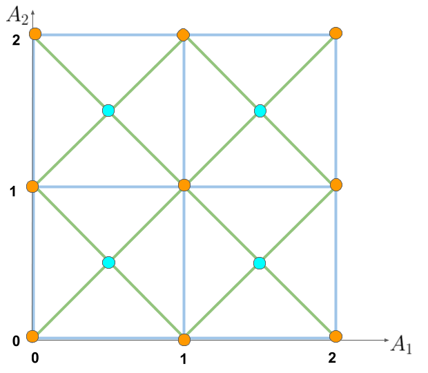
(a) $SO(32)$ heterotic

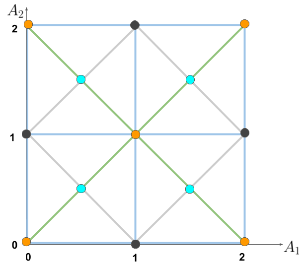
(b) $E_{8}\times E_{8}$ heterotic

Figure 1: Enhancement groups on the left sector of the heterotic theory on the slice of moduli space defined by $A^{3,...,16}=0$, $R=R_{0}$ with a generic $R_{0}>1$

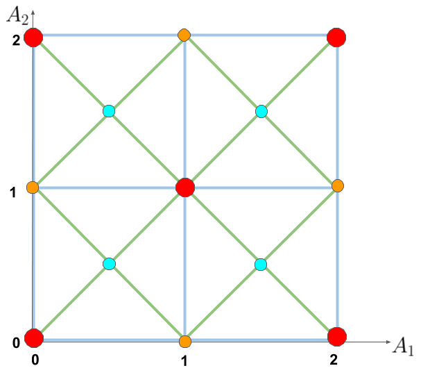
(a) $SO(32)$ heterotic

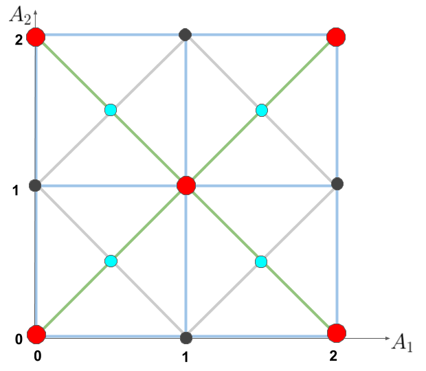
(b) $E_{8}\times E_{8}$ heterotic

Figure 2: Enhancement groups on the left sector of the heterotic theory on the slice of moduli space defined by $A^{3,...,16}=0$, $R=1$.

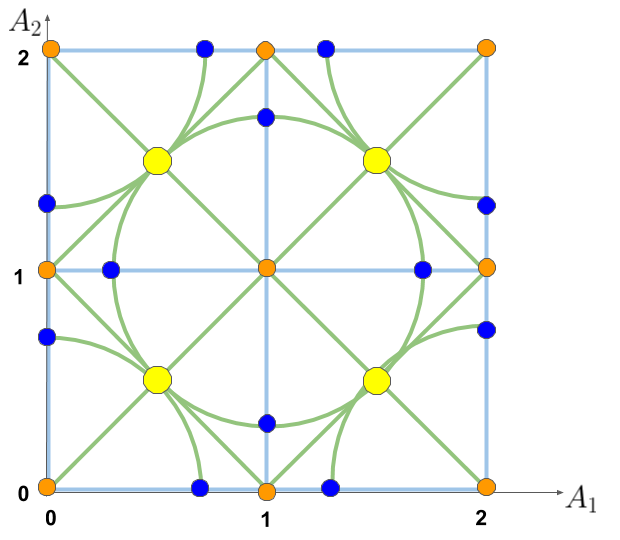
(a) $SO(32)$ heterotic

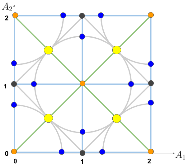
(b) $E_{8}\times E_{8}$ heterotic

Figure 3: Enhancement groups on the left sector of the heterotic theory on the slice of moduli space defined by $A^{3,...,16}=0$, $R^{2}=3/4$.

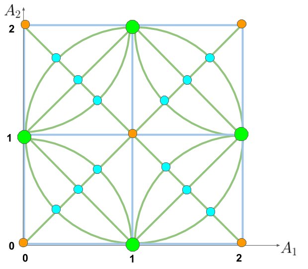
(a) $SO(32)$ heterotic

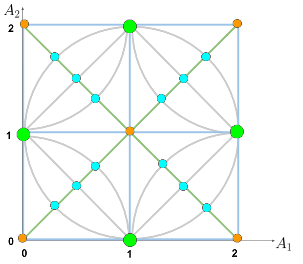
(b) $E_{8}\times E_{8}$ heterotic

Figure 4: Enhancement groups on the left sector of the heterotic theory on the slice of moduli space defined by $A^{3,...,16}=0$, $R^{2}=1/2$.

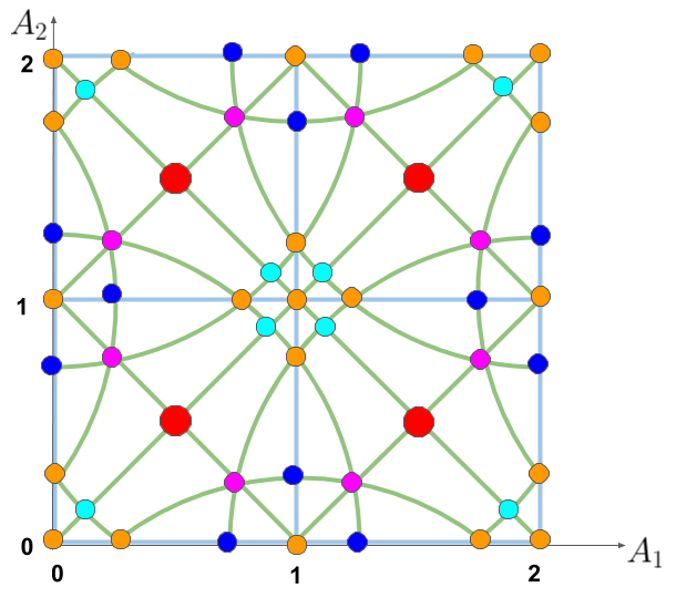
(a) $SO(32)$ heterotic

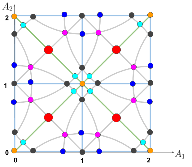
(b) $E_{8}\times E_{8}$ heterotic

Figure 5: Enhancement groups on the left sector of the heterotic theory on the slice of moduli space defined by $A^{3,...,16}=0$, $R^{2}=1/4$.

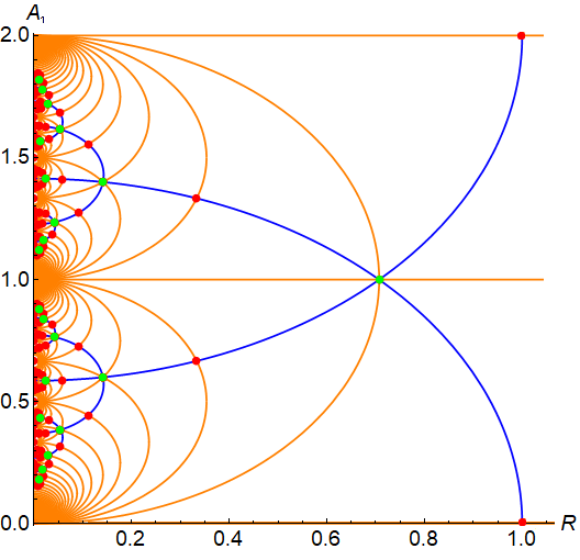
(a) $SO(32)$ heterotic

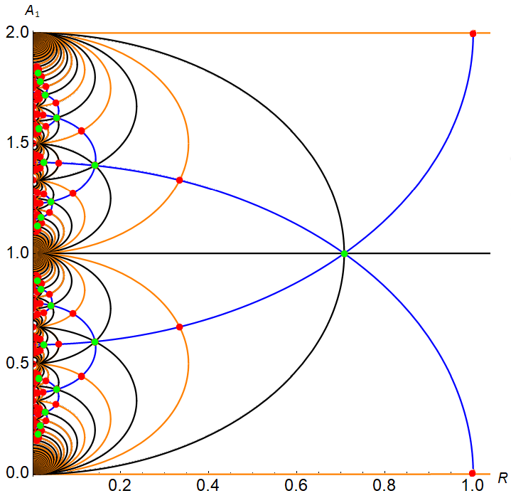
(b) $E_{8}\times E_{8}$ heterotic

Figure 6: Enhancement groups on the left sector of the heterotic theory on the slice of moduli space defined by $A^{2,...,16}=0$.

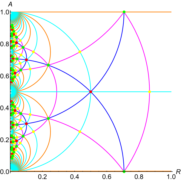
(a) $SO(32)$ heterotic

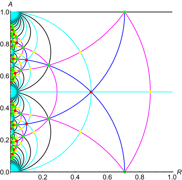
(b) $E_{8}\times E_{8}$ heterotic

Figure 7: Enhancement groups on the left sector of the heterotic theory on the slice of moduli space defined by $A,R$, with Wilson line $A^{I}=\left(A,0_{7},A+1,0_{7}\right)$.

$SO(32)$ heterotic:

$$\text{(\ref{fig:SO32anyR} to \ref{fig:SO32R4})}\,\rightarrow \begin{cases}{\fcolorbox{black}{white}{\rule{0pt}{3pt}\rule{3pt}{0pt}}}\quad U(1)^{3}\times SO(28)\\ {\fcolorbox{black}{verde2}{\rule{0pt}{3pt}\rule{3pt}{0pt}}}\quad U(1)^{2}\times SU(2)\times SO(28)\\ {\fcolorbox{black}{celeste}{\rule{0pt}{3pt}\rule{3pt}{0pt}}}\quad U(1)^{2}\times SO(30)\end{cases}$$

$$\text{(\ref{fig:SO32AR_1})}\,\rightarrow\,{\fcolorbox{black}{white}{\rule{0pt}{3pt}\rule{3pt}{0pt}}} \quad U(1)^{2}\times SO(30)$$

$$\text{(\ref{fig:SO32AR_2})}\,\rightarrow\,{\fcolorbox{black}{white}{\rule{0pt}{3pt}\rule{3pt}{0pt}}} \quad U(1)^{2}\times SU(2)\times SO(28)$$

  $$\quad U(1)\times SU(2)^{2}\times SO(28)$$

  $$\quad U(1)\times SU(3)\times SO(28)$$

  $$\quad U(1)\times SU(2)\times SO(30)$$

  $$\quad U(1)\times SO(32)$$

  $$\quad SU(2)\times SU(3)\times SO(28)$$

  $$\quad SU(2)\times SO(32)$$

  $$\quad SO(34)$$

$E_{8}\times E_{8}$ heterotic:

$$\text{(\ref{fig:E8anyR} to \ref{fig:E8R4})}\,\rightarrow \begin{cases}{\fcolorbox{black}{white}{\rule{0pt}{3pt}\rule{3pt}{0pt}}}\quad U(1)^{3}\times SO(12)\times E_{8}\\ {\fcolorbox{black}{gris}{\rule{0pt}{3pt}\rule{3pt}{0pt}}}\quad U(1)^{2}\times SU(2)\times SU(12)\times E_{8}\\ {\fcolorbox{black}{celeste}{\rule{0pt}{3pt}\rule{3pt}{0pt}}}\quad U(1)^{2}\times SO(14)\times E_{8}\\ {\fcolorbox{black}{verde2}{\rule{0pt}{3pt}\rule{3pt}{0pt}}}\quad U(1)^{2}\times E_{7}\times E_{8}\end{cases}$$

$$\text{(\ref{fig:E8AR_1})}\,\rightarrow\,{\fcolorbox{black}{white}{\rule{0pt}{3pt}\rule{3pt}{0pt}}} \quad U(1)^{2}\times SO(14)\times E_{8}$$

$$\text{(\ref{fig:E8AR_2a})}\,\rightarrow\,{\fcolorbox{black}{white}{\rule{0pt}{3pt}\rule{3pt}{0pt}}} \quad U(1)^{2}\times SU(2)\times SO(12)\times E_{8}$$

  $$\quad U(1)\times SU(2)\times E_{7}\times E_{8}$$

  $$\quad U(1)\times SU(3)\times SO(12)\times E_{8}$$

  $$\quad U(1)\times SU(2)\times SO(14)\times E_{8}$$

  $$\quad U(1)\times SO(16)\times E_{8}$$

  $$\quad U(1)\times E_{8}\times E_{8}$$

  $$\quad SU(3)\times E_{7}\times E_{8}$$

  $$\quad SU(2)\times E_{8}\times E_{8}$$

  $$\quad SO(18)\times E_{8}$$

3.2 Enhancement-breaking of gauge symmetry

Whenever the Wilson line is not in the dual root lattice, part or all of the $SO(32)$ or $E_{8}\times E_{8}$ symmetry is broken. However, this does not imply that no symmetry enhancement from the circle direction is possible. The pattern of gauge symmetries can still be rich. We denote these cases enhancement-breaking of gauge symmetry. This nomenclature can be confusing however: for specific values of $R$ and $A$, there is the possibility that the symmetry enhancement is so large that it restores the original $SO(32)$ or $E_{8}\times E_{8}$ symmetry, or even leads to a larger group of rank 17. This means that we can have a maximal enhancement even if the Wilson line is not in the dual root lattice, either to the groups listed at the end of the previous section, or to any other simply-laced, semi-simple group of rank 17, such as for example $SO(18)\times E_{8}$.

The massless states for an arbitrary Wilson line are the following:

Sector 1 has $w=0$ (and thus $p^{A}=\pi^{A}$) and consists of the roots of $SO(32)$ or $E_{8}\times E_{8}$ satisfying $\pi\cdot A\in\mathbb{Z}$, which form a subgroup $H\subset SO(32)$ or $H\subset E_{8}\times E_{8}$. We give examples of Wilson lines preserving $U(1)\times SU(16)\subset SO(32)$, $SO(2p)\times SO(32-2p)\subset SO(32)$, $U(1)\times SU(p)\times SO(32-2p)\subset SO(32)$, $U(1)\times SU(9)\times SO(16)\subset E_{8}\times E_{8}$, $U(1)^{2}\times SU(8)\times SU(8)\subset E_{8}\times E_{8}$, $SO(16)\times E_{8}\subset E_{8}\times E_{8}$, $SU(2)\times E_{7}\times E_{8}\subset E_{8}\times E_{8}$ in the following sections.

Sector 2 contains states only at radii $R^{2}=s^{2}/(2w^{2})$. Quantization of momentum gives the condition (3.6).If there are states in this sector, there is an enhacement of $H\times U(1)$ to $H\times SU(2)$ (where the $SU(2)$ can be on the circle direction or along some direction mixing the circle with the heterotic directions) or to a group that is not a product, like for example enhancement of $SO(16)\times U(1)$ to $SO(18)$, as we will show in detail.

On figures 6 to 28 sector 1 is represented by the horizontal lines and sector 2 by the curves.

Now we show explicitly how the groups mentioned in sector 1 get enhanced respectively to $SO(34)$ at $R^{2}=\tfrac{1}{2}$; $SU(18)$ at $R^{2}=\tfrac{1}{4}$; $E_{p+1}\times SO(32-2p)$ at $R^{2}=1-\tfrac{p}{8}$; $E_{p+1}\times SU(16-p)$ at $R^{2}=1-\tfrac{8}{16-p}$ in the $SO(32)$ theory, and $SO(34)$ at $R^{2}=\tfrac{1}{18}$; $SU(18)$ at $R^{2}=\tfrac{1}{9}$; $SO(18)\times E_{8}$ at $R^{2}=\frac{1}{2}$; $SU(2)\times E_{8}\times E_{8}$ at $R^{2}=\tfrac{1}{4}$ in the $E_{8}\times E_{8}$.

- Explicit examples for the $\Gamma_{16}$ theory

Here we present some examples of symmetry enhancement-breaking. The roots of $SO(32)$ are given by

$$SO(32)\ :\quad(\underline{\pm 1,\pm 1,0^{14}})\,,$$ (3.7)

where underline means all possible permutations of the entries.

3.2.1 $U(1)\times SO(32)\to SO(34)$

Consider the $SO(32)$ heterotic theory compactified on a circle of radius $R=1/\sqrt{2}$ with a Wilson line $A=(1,0,\dots,0)\in\Gamma_{v}$. The states with $p_{R}=0$ have left-moving momenta

$${\bf p_{L}}=(w,\,\pi^{A}+\delta_{1}^{A}w\,)\,,$$ (3.8)

where the first entry corresponds to the circle direction. In sector 1, with $w=0$, all the momenta satisfy $|\pi^{A}|^{2}=2$ and $\pi\cdot A\in{\mathbb{Z}}$. The last condition holds for any $\pi^{A}\in\Gamma_{g}$, and thus in this sector one has all the root vectors of $SO(32)$ given in (3.7). In sector 2 we have $s=1$ and $w=\pm 1$. Here we get massless states coming from three different sectors of the $SO(32)$ weight lattice, namely

2.a) $|\pi|^{2}=2$, with $\pi^{1}=\pm 1$

$${\bf p_{L}}=(\pm 1,0,\underline{\pm 1,0,0,\dots,0})\qquad$$ (3.9)

(where the signs are not correlated). These are $60$ states with $n=0$.

2.b) $|\pi|^{2}=0$,

$${\bf p_{L}}=(\pm 1,\pm 1,0,\dots,0)\,.\qquad$$ (3.10)

These are 2 states, which have $n=w$.

2.c) $|\pi|^{2}=4$, with $\pi^{1}=\pm 2$

$${\bf p_{L}}=(\mp 1,\pm 1,0,\dots,0)\,.$$ (3.11)

Another $2$ states with $n=-w$.

We thus get 64 extra states, which together with the Cartan direction of the circle, enhance the $SO(32)$ to $SO(34)$. This point in moduli space is illustrated in green in figures 4(a), 6(a) and 7(a). In figure 4(a) the other green points differ from this by a $\Lambda$-shift, while the other green points in figures 6(a) and 7(a), that appear at a different radii, will be explained in section 3.3.

3.2.2 $U(1)^{2}\times SU(16)\to SU(18)$

We now take the Wilson line $A=\left(\left(\tfrac{1}{4}\right)_{15},-\tfrac{3}{4}\right)$. In sector 1 ($w=0$) we have the roots of $SO(32)$ that obey:

$$\tfrac{1}{4}\sum_{A=1}^{16}\pi^{A}-\pi^{16}\in\mathbb{Z}\,.$$ (3.12)

Since the sum cannot be a multiple of $4$, it has to vanish. Then we have the roots with two non-zero entries of opposite signs, that is $SU(16)$. For a generic $R$ this is the gauge group, but if $R^{2}=\tfrac{1}{4}$ we get enhancement to the maximal group $SU(18)$. In this case, the mass formula (3.4) gives

$$\sum_{i=1}^{15}(\pi_{i}+\tfrac{w}{4})^{2}+(\pi_{16}-w+\tfrac{w}{4})^{2}=\sum_{i=1}^{16}(\hat{\pi}_{i}+\tfrac{w}{4})^{2}=2-\tfrac{w^{2}}{2}$$

where we defined $\hat{\pi}=(\pi_{1},\pi_{2},\dots,\pi_{15},\pi_{16}-w)$. If $w$ is even then $\hat{\pi}$ is in $(0)$ or $(s)$, but if it is odd then $\hat{\pi}$ is in $(v)$ or $(c)$. We also have the quantization condition:

$$\frac{\tfrac{1}{2}|\pi|^{2}-1}{w}=\frac{\tfrac{1}{2}|\hat{\pi}|^{2}+\tfrac{1}{2}w^{2}+w\hat{\pi}_{16}-1}{w}=\frac{\tfrac{1}{2}|\hat{\pi}|^{2}-1}{w}+\tfrac{w}{2}+\hat{\pi}_{16}\in\mathbb{Z}\,.$$ (3.13)

For $w=1$, $-\sum_{i=1}^{16}\hat{\pi}_{i}=2|\hat{\pi}|^{2}-1$, and the solutions are $\hat{\pi}=-\left(\underline{1,0_{15}}\right)$ on $(v)$ and $\hat{\pi}=-\left(\underline{(\tfrac{1}{2})_{15},-\tfrac{1}{2}}\right)$ on $(c)$.

For $w=2$, $\sum_{i=1}^{16}(\hat{\pi}_{i}+\tfrac{1}{2})^{2}=0$, with unique solution $\hat{\pi}=-\left(\left(\tfrac{1}{2}\right)_{16}\right)$.

They all obey the quantization condition, and add up to $66$ additional states. Together with the $240$ roots of $SU(16)$, they complete the $306$ roots of $SU(18)$.

3.2.3 $U(1)\times SO(2p)\times SO(32-2p)\to E_{p+1}\times SO(32-2p)$

Now we take a Wilson line $A=\left(\left(\tfrac{1}{2}\right)_{p},0_{16-p}\right)$, $2\leq p\leq 8$, in the SO(32) theory.

The massless states that survive in sector 1 ($w=0$) are those with momentum $\pi^{A}$ satisfying

$$\frac{1}{2}\sum\limits_{A=1}^{p}\pi^{A}\in\mathbb{Z}\,.$$ (3.14)

Then the surviving states have momenta

$${\bf p_{L}} =(0,\underline{\pm 1,\pm 1,0_{p-2}},0_{16-p})\longrightarrow SO(2p)\,,$$ (3.15)

$${\bf p_{L}} =(0,0_{p},\underline{\pm 1,\pm 1,0_{14-p}})\ \ \longrightarrow SO(32-2p)\,.$$

For generic radius there are no states with non-zero winding, and then we get $SO(2p)\times SO(32-2p)$. These points are illustrated for $p=2$ by the cyan dots in figures 1(a), 2(a), 4(a) and 5(a); for $p=7$, on the horizontal cyan line in figure 7(a) and for other values of $p$, at half-integer values of the horizontal lines of the figures in appendix D.

At special values of $R$ some states with non-vanishing winding are massless. For example, when $R^{2}=1-\frac{p}{8}$ for $p<8$, the $U(1)\times SO(2p)$ is enhanced to $E_{p+1}$. In this case, the mass formula (3.4) is

$$\sum_{i=1}^{p}(\pi_{i}+\tfrac{w}{2})^{2}+\sum_{i=p+1}^{16}\pi_{i}^{2}=2-2w^{2}(1-p/8)\leq\frac{p}{4}\,,$$

and then if $p<8$ the lhs must be smaller than $2$. If the $\pi_{i}$ are semi-integer, then the lhs is always bigger than $2$. Consequently, $\pi_{i}$ can only take integer values and we need $\sum_{i=p+1}^{16}\pi_{i}^{2}=\beta=0,\,1$.

For $w=1$ the solution must be of the form $\left(\underline{(-1)_{k},0_{p-k}},\underline{\pm\beta,0_{15-p}}\right)$ and the equation is solved for every $p$ if $\beta=0$. Then we get $\left(\underline{(-1)_{k},0_{p-k}},0_{16-p}\right)$.

There is an additional constraint because $|\pi|^{2}$ must be even, and then $k$ must be even. The number of states is equal to the way of choosing the value of the first $p$ components. Choosing the first $p-1$ components, the last one is fixed by the constraint. There are $2\times 2^{p-1}=2^{p}$ states with $|w|=1$.

For $w=2$ we get $\sum_{i=1}^{p}(\pi_{i}+1)^{2}=p-6-\beta$, which is only possible for $p=6,\,7$. The rhs can only take the values $0$ or $1$. In the first case, all the $\pi_{i}$ must be equal to $-1$. Then we get the solutions $\left((-1)_{7},\underline{\pm 1,0_{8}}\right)$ for $p=7$ and $\left((-1)_{6},0_{10}\right)$ for $p=6$ . The second case is only possible for $p=7$ and $\beta=0$. One of the $\pi_{i}$ can take the value $0$ (or $-2$) and the rest must take the value $-1$: $\left(\underline{-1\pm 1,(-1)_{6}},0_{9}\right)$ for $p=7$. In total we have $2$ states with $|w|=2$ for $p=6$ and $2\times(18+14)=64$ for $p=7$.

For $w\geq 3$ the equation cannot be satisfied. Then for $p<6$ we get $2^{p}$ states (all with $|w|=1$), while for $p=6$ and $7$ we get $2$ and $64$ extra states respectively with $|w|=2$.

$$U(1)\times SO(4)\rightarrow SU(2)\times SU(3)\equiv E_{3}\text{ (4 extra states)}$$ (3.16)

$$U(1)\times SO(6)\rightarrow SU(5)\equiv E_{4}\text{ (8 extra states)}$$

$$U(1)\times SO(8)\rightarrow SO(10)\equiv E_{5}\text{ (16 extra states)}$$

$$U(1)\times SO(10)\rightarrow E_{6}\text{ (32 extra states)}$$

$$U(1)\times SO(12)\rightarrow E_{7}\text{ (66 extra states)}$$

$$U(1)\times SO(14)\rightarrow E_{8}\text{ (192 extra states)}$$

Recalling that $E_{2}=U(1)\times SU(2)$, this is also valid for $p=1$, where we get the enhancement at $R^{2}=\tfrac{7}{8}$:

$$U(1)^{2}\equiv U(1)\times SO(2)\rightarrow U(1)\times SU(2)\equiv E_{2}\text{ (2 extra states)}\,.$$ (3.17)

The enhancement group $U(1)\times SU(2)\times SO(30)$, as any non-maximal enhancement, does not arise at an isolated point, but at a line, displayed in blue in figure 6(a).

Applying the statement to $p=8$, appears an enhancement from $U(1)\times SO(16)$ to $E_{9}$ at $R=0$. Since $E_{9}$ has infinite dimension, we would need infinite massless states with infinitely many different winding numbers. It is obvious that at $R=0$ winding states do not cost any energy, and thus one can have all the windings. The mass equation is:

$$\sum_{i=1}^{8}(\pi_{i}+\tfrac{w}{2})^{2}=2-\beta\,.$$ (3.18)

We see that for this value of $p$ the rhs is independent of the winding number. If $w=1$ then $\pi=\left(\underline{(-1)_{k},0_{8-k}},0_{8}\right)$ is a solution (if $k$ is even). For any other odd value of $w$ we have the solution: $\pi=-\left(\underline{\left(\frac{w+1}{2}\right)_{k},\left(\frac{w-1}{2}\right)_{8-k}},0_{8}\right)$. These, together with the states with even $w$, give infinite massless states.

We can see all these enhancements at the intersections of the lines at $A=1/2$ in figures 9 to 24 that occur at $R^{2}=1-\tfrac{p}{8}$.

3.2.4 $U(1)^{2}\times SO(2p)\times SU(16-p)\to SU(2)\times E_{p+1}\times SU(16-p)$

Consider the Wilson line $A=\left(\left(\tfrac{4}{16-p}\right)_{p},0_{p}\right)$, with $0\leq p\leq 7$.

The massless states that survive in sector 1 ($w=0$) are those with momentum $\pi^{A}$ satisfying $\frac{4}{16-p}\sum\limits_{A=1}^{16-p}\pi^{A}\in\mathbb{Z}.$ Then the surviving states have momenta

$${\bf p_{L}} =(0,0_{16-p},\underline{\pm 1,\pm 1,0_{p+2}})\longrightarrow SO(2p)$$ (3.19)

$${\bf p_{L}} =(0,\underline{1,-1,0_{14-p}},0_{p})\ \ \longrightarrow SU(16-p)$$

For generic radii there cannot be states with non-zero winding, and then the symmetry group is $SO(2p)\times SU(16-p)$. This is illustrated in the white spaces of the figures in Appendix D.

There are special values of $R$ where some states with non-vanishing winding are massless. For example, when $R^{2}=1-\frac{8}{16-p}$, the $U(1)^{2}\times SO(2p)$ is enhanced to $SU(2)\times E_{p+1}$. To see this, consider the mass formula (3.4)

$$\sum_{i=1}^{q}(\pi_{i}+\tfrac{4w}{q})^{2}+\sum_{i=q+1}^{16}\pi_{i}^{2}=2-2w^{2}(1-8/q)\,\ {\rm where}\ q\equiv 16-p\ .$$

For $w\neq 0$, the rhs is smaller than or equal to $16/q$ and then the lhs must be smaller than $2$. If the $\pi_{i}$ are integer, then we need $\sum_{i=q+1}^{16}\pi_{i}^{2}=\beta=0,\,1$ and it follows that

$$\sum_{i=1}^{q}(\pi_{i}+\tfrac{4w}{q})^{2}=2-2w^{2}(1-8/q)-\beta\,.$$

For $w=1$, $\sum_{i=1}^{q}(\pi_{i}+\tfrac{4}{q})^{2}=16/q-\beta\leq\tfrac{16}{9}$. If one of the $\pi_{i}$ is different from $0$ or $-1$ then the lhs is larger than $16/q$. So the solution must be of the form $\left(\underline{(-1)_{k},0_{16-p-k}},\underline{\pm\beta,0_{p-1}}\right)$ and then $k=\beta=0$. There are only two states (considering also $w=-1$) with momentum $\left(0_{16}\right)$.

For $w=2$ we get $\sum_{i=1}^{q}(\pi_{i}+8/q)^{2}=-6+64/q-\beta$ which is only possible for $q=9,\,10$ ($p=7,6$). If $p=6$ then we need $\beta=0$, the rhs is $\tfrac{2}{5}$ and we only have the solution $\left((-1)_{10},0_{6}\right).$ If $p=7$ then, for $\beta=0$ and $\beta=1$ the rhs takes the values $\tfrac{10}{9}$ and $\tfrac{1}{9}$. The equation for $\beta=0$ is impossible to satisfy, and then we get $\left((-1)_{9},\underline{\pm 1,0_{6}}\right)$. In total we have $2$ states with $|w|=2$ for $p=6$ and $2\times(14)=28$ for $p=7$.

For $w\geq 3$ we get $\sum_{i=1}^{q}(\pi_{i}+12/q)^{2}=144/q-16-\beta\leq 0$. Then for $q>10$ ($p<6$) there are $2$ states (both with $|w|=1$), while for $p=6$ and $7$ there are $2$ and $28$ extra $|w|=2$ states respectively.

If the $\pi_{i}$ are semi-integer, then the last $p$ values have to be $\pm\tfrac{1}{2}$:

$$\sum_{i=1}^{q}(\pi_{i}+\tfrac{4w}{q})^{2}=\tfrac{q}{4}-2-2w^{2}(1-8/q)$$ (3.20)

For $w=1$, $\sum_{i=1}^{q}(\pi_{i}+\tfrac{4}{q})^{2}=\tfrac{(q-8)^{2}}{4q}\leq 1$ and the $\pi_{i}$ can only take the values $\pm\tfrac{1}{2}$. The solutions are of the form $\left(\underline{\left(\tfrac{1}{2}\right)_{k},\left(-\tfrac{1}{2}\right)_{16-p-k}},\underline{\left(\pm\tfrac{1}{2}\right)_{p}}\right)$, and the equation implies $k=0$. Then, for $|w|=1$, we get the $2\times 2^{p+1+\delta_{p,0}}$ solutions $\left(\left(-\tfrac{1}{2}\right)_{16-p},\underline{\left(\pm\tfrac{1}{2}\right)_{p}}\right)$.

For $w=2$ we obtain $\sum_{i=1}^{q}(\pi_{i}+\tfrac{8}{q})^{2}=\tfrac{(q-8)(q-32)}{4q}\leq 0$, and then there are no states with $|w|>1$.

In total, for $p<6$ we get $2+2^{p+\delta_{p,0}}$ states (all of them with $|w|=1$), while for $p=6$ and $7$ we get $2$ and $28$ extra states respectively with $|w|=2$.

$$U(1)^{2}\rightarrow SO(4)\equiv SU(2)\times E_{1}\text{ (4 extra states)}$$

$$U(1)^{3}\equiv U(1)^{2}\times SO(2)\rightarrow SU(2)\times SU(2)\times U(1)\equiv SU(2)\times E_{2}\text{ (4 extra states)}$$

$$U(1)^{2}\times SO(4)\rightarrow SU(2)\times SU(2)\times SU(3)\equiv SU(2)\times E_{3}\text{ (6 extra states)}$$

$$U(1)^{2}\times SO(6)\rightarrow SU(2)\times SU(5)\equiv SU(2)\times E_{4}\text{ (10 extra states)}$$

$$U(1)^{2}\times SO(8)\rightarrow SU(2)\times SO(10)\equiv SU(2)\times E_{5}\text{ (18 extra states)}$$

$$U(1)^{2}\times SO(10)\rightarrow SU(2)\times E_{6}\text{ (34 extra states)}$$

$$U(1)^{2}\times SO(12)\rightarrow SU(2)\times E_{7}\text{ (68 extra states)}$$

$$U(1)^{2}\times SO(14)\rightarrow SU(2)\times E_{8}\text{ (158 extra states)}$$

At $p=8$ we seem to get an enhancement from $U(1)^{2}\times SO(16)$ to $SU(2)\times E_{9}$ at $R=0$.

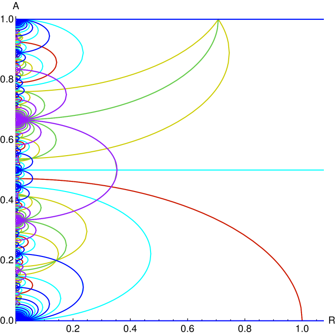
  $$\quad SU(9)\times SO(14)\times U(1)^{2}$$

  $$\quad SU(2)\times SU(9)\times U(1)\times SO(14)$$

  $$\quad SU(10)\times SO(14)\times U(1)$$

  $$\quad SO(18)\times SO(14)\times U(1)$$

  $$\quad SU(9)\times SO(16)\times U(1)$$

  $$\quad SO(32)\times U(1)$$

  $$\quad SU(9)\times E_{8}\times U(1)$$

$${\fcolorbox{black}{azul}{\rule{0pt}{3pt}\rule{3pt}{0pt}}}+{\fcolorbox{black}{verde}{\rule{0pt}{3pt}\rule{3pt}{0pt}}}+{\fcolorbox{black}{amarillo}{\rule{0pt}{3pt}\rule{3pt}{0pt}}}+{\fcolorbox{black}{amarillo}{\rule{0pt}{3pt}\rule{3pt}{0pt}}} \quad SO(34)$$

$${\fcolorbox{black}{violeta}{\rule{0pt}{3pt}\rule{3pt}{0pt}}}+{\fcolorbox{black}{cyan}{\rule{0pt}{3pt}\rule{3pt}{0pt}}} \quad SO(18)\times E_{8}$$

$${\fcolorbox{black}{violeta}{\rule{0pt}{3pt}\rule{3pt}{0pt}}}+{\fcolorbox{black}{amarillo}{\rule{0pt}{3pt}\rule{3pt}{0pt}}} \quad SU(10)\times E_{8}$$

$${\fcolorbox{black}{violeta}{\rule{0pt}{3pt}\rule{3pt}{0pt}}}+{\fcolorbox{black}{rojo}{\rule{0pt}{3pt}\rule{3pt}{0pt}}} \quad SU(2)\times SU(9)\times E_{8}$$

$${\fcolorbox{black}{azul}{\rule{0pt}{3pt}\rule{3pt}{0pt}}}+{\fcolorbox{black}{rojo}{\rule{0pt}{3pt}\rule{3pt}{0pt}}} \quad SU(2)\times SO(32)$$

Figure 17: $SO(32)$ heterotic with Wilson line $A^{I}=\left((A)_{9},0_{7}\right)$

All of these enhancements can be seen on the intersections of the red and purple curves of figures 17 to 24 that occur at $R^{2}=1-\tfrac{8}{q}$.

- Explicit examples for the $\Gamma_{8}\times\Gamma_{8}$ theory

The roots of $E_{8}\times E_{8}$ are

$$E_{8}\times E_{8}\ : (\underline{\pm 1,\pm 1,0^{6}},0^{8})\,,\ (0^{8},\underline{\pm 1,\pm 1,0^{6}})\ ,\$$

$$((\pm\frac{1}{2})^{8},0^{8})\,,\ (0^{8},(\pm\frac{1}{2})^{8})\ ,\rm{with\ even\ number\ of\ +\ signs}$$

3.2.5 $U(1)^{2}\times SU(9)\times SO(16)\to SO(34)$

Consider the $\Gamma_{8}\times\Gamma_{8}$ theory compactified with Wilson line $A=\left(\left(\tfrac{1}{6}\right)_{7},\tfrac{5}{6},1,0_{7}\right)$. In sector 1 ($w=0$) we have the roots of $E_{8}\times E_{8}$ that obey:

$$\tfrac{1}{6}\sum_{A=1}^{7}\pi^{A}+\tfrac{5}{6}\pi^{8}+\pi^{9}\in\mathbb{Z}$$ (3.22)

This breaks into two conditions, one for each $E_{8}$:

$$\tfrac{1}{6}\sum_{A=1}^{7}\pi^{A}+\tfrac{5}{6}\pi^{8}\in\mathbb{Z}\,\qquad{\rm and}\qquad\pi^{9}\in\mathbb{Z}\,.$$ (3.23)

For the first condition we have $(0)$ and $(s)$ roots. The $(0)$ roots are vectors of the form $\left(\underline{\pm 1,\pm 1,0_{6}}\right)$. The condition implies that if $\pi_{8}=0$ then we need opposite signs for the two non-zero entries. If $\pi^{8}=\pm 1$ then the other non-zero entry must have the same sign. We get $\left(\underline{1,-1,0_{5}},0\right)$ and $\pm\left(\underline{1,0_{6}},1\right)$. These are $42+14=56$ roots.

The $(s)$ roots are vectors of the form $\left(\underline{\left(\pm\tfrac{1}{2}\right)_{8}}\right)$ with an even number of minus signs. The condition is $\sum_{A=1}^{7}\pi^{A}+5\pi^{8}=0$ mod $6$. The absolute value of the lhs can only be $0$ or $6$. In the first case one of the first $5$ components must have a different sign than the rest, and in the second case all the $8$ components must have the same sign and we get $\pm\left(\underline{\left(\tfrac{1}{2}\right)_{6},-\tfrac{1}{2}},-\tfrac{1}{2}\right)$ and $\pm\left(\left(\tfrac{1}{2}\right)_{8}\right)$. These are $14+2=16$ roots.

In total we have the $56+16=72$ roots of $SU(9)$.

The second condition leaves only the integer roots, and then we have $SO(16)$.

For an arbitrary value of $R$ there cannot be states with non-zero winding, and then the gauge group is $SU(9)\times SO(16)$.

Now we show that when $R^{2}=\tfrac{1}{18}$ there is enhancement of the gauge symmetry to $SO(34)$. The mass formula (3.4) is:

$$\sum_{i=1}^{7}(\pi_{i}+\tfrac{w}{6})^{2}+(\pi_{8}+\tfrac{5w}{6})^{2}+(\pi_{9}+w)^{2}+\sum_{i=10}^{16}\pi_{i}^{2}=2-\tfrac{w^{2}}{9}<2\,.$$ (3.24)

Then $\sum_{i=10}^{16}\pi_{i}^{2}$ can only take the values $0$, $1$ or $\tfrac{7}{4}$. In the last case, we also have that $(\pi_{9}+w)^{2}\geq\tfrac{1}{4}$, which means that there are no spinorial roots in the last $8$ components. The only possibilities are: $\left(-w,0_{7}\right)$ and $\left(-w,0_{7}\right)\pm\left(\underline{1,0_{7}}\right)$. The first (second) case requires $w$ to be even (odd). Defining $\hat{\pi}=\left(\pi_{1},\pi_{2},\dots,\pi_{7},-\pi_{8}-w\right)$, we have:

$$\sum_{i=1}^{8}(\hat{\pi}_{i}+\tfrac{w}{6})^{2}=2-\tfrac{w^{2}}{9}-\tfrac{1-(-1)^{w}}{2}$$ (3.25)

but now the condition for the integer vectors is $\sum_{i=1}^{8}\hat{\pi}_{i}$ odd (even) when $w$ is odd (even); and for the half-integer vectors we have the $(s)$ conditions if $w$ is odd and the $(c)$ conditions if $w$ is even.

The quantization condition is

$$\frac{\tfrac{1}{2}|\pi|^{2}-1}{w}\in\mathbb{Z}\rightarrow\begin{cases}|\pi|^{2}=0\text{ mod }2&\text{ for }|w|=1\\ |\pi|^{2}=2\text{ mod }4&\text{ for }|w|=2\\ |\pi|^{2}=2\text{ mod }6&\text{ for }|w|=3\end{cases}$$ (3.26)

If $w=1$, $-\sum_{i=1}^{8}\hat{\pi}_{i}=3|\hat{\pi}_{i}|^{2}-2.$ The minimum value for $|\hat{\pi}_{i}|^{2}$ is $1$, and in that case we have $\hat{\pi}=-\left(\underline{1,0_{7}}\right)$.

$|\hat{\pi}_{i}|^{2}=2$ can only be achieved for the $(s)$ conjugacy class, and then $\hat{\pi}=-\left(\left(\tfrac{1}{2}\right)_{8}\right)$.

$|\hat{\pi}|^{2}=3$ is for the $(v)$ conjugacy class, $-\sum_{i=1}^{8}\hat{\pi}_{i}=7$, but this cannot be achieved. The same happens for greater values of $|\hat{\pi}|^{2}$.

If $w=2$, $-\sum_{i=1}^{8}\hat{\pi}_{i}=\tfrac{3}{2}|\hat{\pi}_{i}|^{2}-1$. Then $|\hat{\pi}|^{2}$ has to be even. The minimum value is $0$, which could be achieved only on $(0)$, and the equation cannot be solved. $|\hat{\pi}|^{2}=2$ can only be achieved for $(0)$ and we get $\left(\underline{(-1)_{2},0_{6}}\right)$. $|\hat{\pi}|^{2}=4$ has the solution $\hat{\pi}=-\left(\underline{\tfrac{3}{2},(\tfrac{1}{2})_{7}}\right)$. And for $|\hat{\pi}|^{2}=6$ the equation cannot be satisfied.

If $w=3$, $\sum_{i=1}^{8}(\hat{\pi}_{i}+\tfrac{1}{2})^{2}=0$, and the only solution is $\hat{\pi}=\left(\left(-\tfrac{1}{2}\right)_{8}\right)$. That is $\pi=\left((-\tfrac{1}{2})_{7},-\tfrac{5}{2},-3,0_{7}\right)+\left(0_{8},\underline{\pm 1,0_{7}}\right)$. This has $|\pi|^{2}=12$, $18$ or $24$, which do not obey the quantization condition.

If $w=4$, $-\sum_{i=1}^{8}\hat{\pi}_{i}=\tfrac{3}{4}|\hat{\pi}|^{2}+\tfrac{1}{6}$. But this equation cannot be solved for integer $|\hat{\pi}|^{2}$.

Defining $8$ more components for a $16$ dimensional $\hat{\pi}$ such that $\hat{\pi}_{9}=\pi_{9}-w$ and the rest equal to the last $7$ components of $\pi$, one can write the additional states $\hat{\pi}$ for $R^{2}=\tfrac{1}{18}$ as $\left(\underline{\pm 1,0_{7}},\underline{\pm 1,0_{7}}\right)$ and $\left(\pm\left(\tfrac{1}{2}\right)_{8},\underline{\pm 1,0_{7}}\right)$ for $|w|=1$ and $\pm\left(\underline{(1)_{2},0_{6}},0_{8}\right)$ and as $\pm\left(\left(\underline{\tfrac{3}{2},(\tfrac{1}{2})_{7}}\right),0_{8}\right)$ for $|w|=2$. The former are $256+32=288$ states and the latter $56+16=72$ states. In total these $360$ additional states added to the $184$ roots of $SU(9)\times SO(16)$ give the $544$ roots of $SO(34)$.

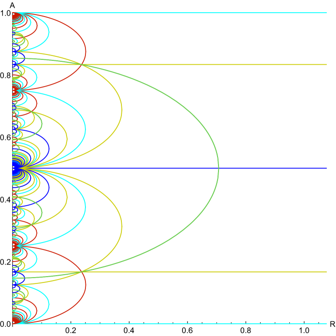
  $$\quad SU(8)\times SO(16)\times U(1)^{2}$$

  $$\quad SO(32)\times U(1)$$

  $$\quad SO(16)\times SO(16)\times U(1)$$

  $$\quad SU(9)\times SO(16)\times U(1)$$

  $$\quad E_{8}\times SO(16)\times U(1)$$

  $$\quad SU(8)\times SO(18)\times U(1)$$

$${\fcolorbox{black}{rojo}{\rule{0pt}{3pt}\rule{3pt}{0pt}}}+{\fcolorbox{black}{amarillo}{\rule{0pt}{3pt}\rule{3pt}{0pt}}}+{\fcolorbox{black}{amarillo}{\rule{0pt}{3pt}\rule{3pt}{0pt}}}+{\fcolorbox{black}{verde}{\rule{0pt}{3pt}\rule{3pt}{0pt}}} \quad SO(34)$$

$${\fcolorbox{black}{azul}{\rule{0pt}{3pt}\rule{3pt}{0pt}}}+{\fcolorbox{black}{verde}{\rule{0pt}{3pt}\rule{3pt}{0pt}}} \quad E_{8}\times SO(18)$$

Figure 26: $\Gamma_{8}\times\Gamma_{8}$ heterotic with Wilson line $A^{I}=\left((A)_{7},1-A,1,0_{7}\right)$

In figure 26 we show this maximal enhancement on the intersection between one red, two yellow and one green curves. The integer states with $|w|=1$ and $|w|=2$ give the red curve, the half-integer states with $|w|=1$ give the green curve and the ones with $|w|=2$ are represented by the yellow curve. The additional states without winding are those in the yellow line.

3.2.6 $U(1)^{3}\times SU(8)\times SU(8)\to SU(18)$

Consider the Wilson line $A=\left(\left(\tfrac{1}{6}\right)_{7},\tfrac{5}{6},\left(\tfrac{1}{6}\right)_{7},\tfrac{5}{6}\right)$ in the $\Gamma_{8}\times\Gamma_{8}$ theory.

In sector 1 ($w=0$) we have the first condition of (3.23) for each of the $E_{8}$, then we get the $144$ roots of $SU(9)\times SU(9)$. For an arbitrary value of $R$ this is the gauge group.

For $R^{2}=\tfrac{1}{9}$ there is enhancement of the gauge symmetry to $SU(18)$. To see this, take the mass formula (3.4)

$$\sum_{i=1}^{7}(\pi_{i}+\tfrac{w}{6})^{2}+(\pi_{8}+\tfrac{5w}{6})^{2}+\sum_{i=9}^{15}(\pi_{i}+\tfrac{w}{6})^{2}+(\pi_{16}+\tfrac{5w}{6})^{2}=2-\tfrac{2w^{2}}{9}<2\,.$$ (3.27)

Defining $\hat{\pi}=\left(\pi_{1},\pi_{2},\dots,\pi_{7},-\pi_{8}-w,\pi_{9},\pi_{10},\dots,\pi_{15},-\pi_{16}-w\right)$ we have:

$$\sum_{i=1}^{16}(\hat{\pi}_{i}+\tfrac{w}{6})^{2}=2-\tfrac{2w^{2}}{9}\,,$$ (3.28)

but now $\hat{\pi}$ has to be on the conjugacy classes $(ss)$, $(vv)$, $(sv)$ or $(vs)$ if $w$ is odd and on $(cc)$, $(00)$, $(0c)$, $(c0)$ if $w$ is even.

We also have to obey the quantization condition $\frac{\tfrac{1}{2}|\pi|^{2}-1}{w}\in\mathbb{Z}$.

If $w=1$, $-\sum_{i=1}^{16}\hat{\pi}_{i}=3|\hat{\pi}|^{2}-4$ and $\hat{\pi}$ is on $(vv)$, $(ss)$, $(vs)$ or $(sv)$. The minimum value for $|\hat{\pi}_{i}|^{2}$ is $2$, and in that case $(\hat{\pi},\hat{\pi}^{\prime})=-\left(\underline{1,0_{7}},\underline{1,0_{7}}\right)$.

$|\hat{\pi}|^{2}=3$ can only be achieved for the $(vs)$ and $(sv)$ conjugacy classes, and $\hat{\pi}=-\left(\underline{1,0_{7}},(\tfrac{1}{2})_{8}\right)$, $-\left((\tfrac{1}{2})_{8},\underline{1,0_{7}}\right)$. $|\hat{\pi}|^{2}=4$ is for the $(ss)$ and $(vv)$ conjugacy classes, and $\hat{\pi}=-\left((\tfrac{1}{2})_{16}\right)$. $|\hat{\pi}|^{2}=5$ is for the $(sv)$ and $(vs)$ conjugacy classes, $-\sum_{i=1}^{16}\hat{\pi}_{i}=11$ which cannot be achieved. The same happens for greater values of $|\hat{\pi}|^{2}$.

If $w=2$, $-\sum_{i=1}^{16}\hat{\pi}_{i}=\tfrac{3}{2}|\hat{\pi}|^{2}+1$ implies $(00)$, $(cc)$, $(c0)$ or $(0c)$. The minimum value for $|\hat{\pi}_{i}|^{2}$ is $0$, but then the equation cannot be solved.

$|\hat{\pi}|^{2}=2$ can only be achieved for $(00)$, $(0c)$ or $(c0)$, but there is no solution.

$|\hat{\pi}|^{2}=4$ implies $-\sum_{i=1}^{16}\hat{\pi}_{i}=7$ and this cannot be achieved. The same happens for greater values of $|\hat{\pi}|^{2}$.

If $w=3$, $\sum_{i=1}^{16}(\hat{\pi}_{i}+\tfrac{1}{2})^{2}=0$ has only a solution belonging to $(ss)$, namely $\hat{\pi}=-\left(\left(\tfrac{1}{2}\right)_{16}\right)$.

It can be shown that all of these states obey the quantization condition. Then, the additional states for $R^{2}=\tfrac{1}{18}$ are $\pm\left(\underline{1,0_{7}},\underline{1,0_{7}}\right)$, $\pm\left(\underline{1,0_{7}},(\tfrac{1}{2})_{8}\right)$ and $\pm\left((\tfrac{1}{2})_{8},\underline{1,0_{7}}\right)$ for $|w|=1$ and $\hat{\pi}=\left(\left(-\tfrac{1}{2}\right)_{16}\right)$ for $|w|=3$ $\left(\underline{\pm 1,0_{7}},\underline{\pm 1,0_{7}}\right)$ and $\left(\pm\left(\tfrac{1}{2}\right)_{8},\underline{\pm 1,0_{7}}\right)$ for $|w|=1$ and $\pm\left(\underline{(1)_{2},0_{6}},0_{8}\right)$ and $\pm\left(\left(\tfrac{1}{2}\right)_{16}\right)$ for $|w|=2$. The former are $128+32=160$ states and the latter $2$ states. In total these are $162$ additional states, which added to the $144$ roots of $SU(9)\times SU(9)$ give the $306$ roots of $SU(18)$.

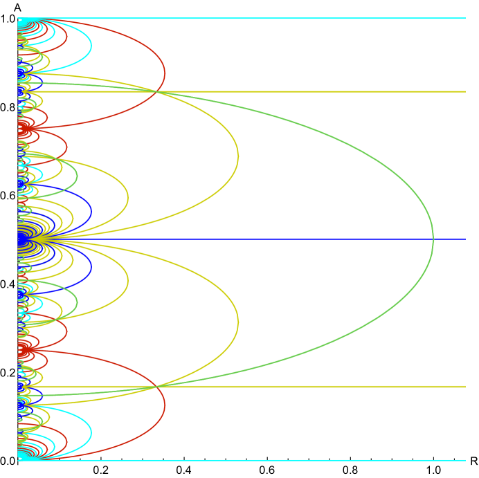
  $$\quad SU(8)\times SU(8)\times U(1)^{3}$$

  $$\quad SU(16)\times U(1)^{2}$$

  $$\quad SO(16)\times SO(16)\times U(1)$$

  $$\quad SU(9)\times SU(9)\times U(1)$$

  $$\quad E_{8}\times E_{8}\times U(1)$$

  $$\quad SU(8)\times SU(8)\times SU(2)\times U(1)$$

$${\fcolorbox{black}{rojo}{\rule{0pt}{3pt}\rule{3pt}{0pt}}}+{\fcolorbox{black}{amarillo}{\rule{0pt}{3pt}\rule{3pt}{0pt}}}+{\fcolorbox{black}{amarillo}{\rule{0pt}{3pt}\rule{3pt}{0pt}}}+{\fcolorbox{black}{verde}{\rule{0pt}{3pt}\rule{3pt}{0pt}}} \quad SU(18)$$

$${\fcolorbox{black}{azul}{\rule{0pt}{3pt}\rule{3pt}{0pt}}}+{\fcolorbox{black}{verde}{\rule{0pt}{3pt}\rule{3pt}{0pt}}} \quad E_{8}\times E_{8}\times SU(2)$$

Figure 27: $\Gamma_{8}\times\Gamma_{8}$ heterotic with Wilson line $A^{I}=\left((A)_{7},1-A,(A)_{7},1-A\right)$

In figure 27 we show this maximal enhancement on the intersection between one red, two yellow and one green curves. The integer states with $|w|=1$ are represented by the red curve, the half-integer states with $|w|=1$ give the yellow curve, the states with $|w|=3$ are represented by the green curve and the additional states with $w=0$ give the yellow horizontal line.

3.2.7 $U(1)\times SO(16)\times E_{8}\to SO(18)\times E_{8}$

Consider the $E_{8}\times E_{8}$ heterotic string compactified on a circle of radius $R=\frac{1}{\sqrt{2}}$, with Wilson line $A=\left(1,0^{7},0^{8}\right)$, which is of the form $(v0)$ according to the notation of Appendix A (see (A.10) in particular). This Wilson line leaves the second $E_{8}$ unbroken, while from the first $E_{8}$, the surviving states in sector 1 are the ones with integer entries, i.e. those in the first line of (3.2.4). The group $H$ from sector 1 is then $SO(16)\times E_{8}$ and the corresponding points in moduli space are illustrated by the grey dots in figure 1(b).

In sector 2 we have states with $w=\pm 1$ such that $s=1$, $|{\bf p}^{A}|^{2}=1$. The surviving states have the following momenta

$${\bf p_{L}}=(0,\underline{\pm 1,\pm 1,0_{6}}),\,w=0,\,|\pi|^{2}=2\quad\text{ $112$ roots}$$

$${\bf p_{L}}=(\pm 1,0,\underline{\pm 1,0_{6}}),\,w=\pm 1,|\pi|^{2}=2,\ \text{ $28$ roots}$$

$${\bf p_{L}}=(\pm 1,\pm 1,0_{7}),\,\ \ \ w=\pm 1,\pi=0,\qquad\text{$2$ roots}$$

$${\bf p_{L}}=(\pm 1,\mp 1,0_{7}),\,\ \ \ w=\pm 1,|\pi|^{2}=4,\quad\text{$2$ roots}\,,$$

where the first entry corresponds to the circle and the subsequent ones to the 8 directions along the Cartan of the first $E_{8}$ factor. The first line contains the states of sector 1. These are the 144 roots of SO(18). This point in moduli space, together with its equivalent ones, are illustrated by the green dots in figure 4(b), 6(b) and 7(b).

3.2.8 $U(1)\times SU(2)\times E_{7}\times E_{8}\to SU(2)\times E_{8}\times E_{8}$

This is an interesting example of enhancement-breaking in the $E_{8}\times E_{8}$ heterotic theory, where first the $E_{8}$ is broken to $SU(2)\times E_{7}$ by the Wilson line $A=\left(\left(\frac{1}{4}\right)_{8},0_{8}\right)$ and then enhanced by the circle direction to $SU(2)\times E_{8}$.

The Wilson line leaves the second $E_{8}$ unbroken, while the surviving roots from the first $E_{8}$ have 9-momenta

$${\bf p_{L}} =\pm(0,\underline{1,-1,0_{6}})$$ (3.29)

$${\bf p_{L}} =\pm\left(0,\left(\tfrac{1}{2}\right)_{8}\right)$$

$${\bf p_{L}} =\left(0,\underline{\left(\tfrac{1}{2}\right)_{4},-\left(\tfrac{1}{2}\right)_{4}}\right)$$

This, gives 128 roots, which together with the 8 Cartan directions, gives an unbroken gauge group $H=SU(2)\times E_{7}\subset E_{8}$.

Additionally at $R=\frac{1}{2}$ there are $114$ states in sector 2: two with $w=\pm 2$ and 112 with $w=\pm 1$ and momentum

$${\bf p_{L}} =\left(\pm\tfrac{\sqrt{2}}{2},\underline{\mp\left(\tfrac{3}{4}\right)_{2},\pm\left(\tfrac{1}{4}\right)_{6}}\right)$$ (3.30)

$${\bf p_{L}} =\left(\pm\tfrac{\sqrt{2}}{2},\underline{\pm\left(\tfrac{3}{4}\right)_{2},\mp\left(\tfrac{1}{4}\right)_{6}}\right)$$

These states give a total of 114 extra states that add up to the previous 136 states, plus the circle direction, adding up to the 251 states of $SU(2)\times E_{8}$. So at $R=\frac{1}{2}$ we get enhancement to $SU(2)\times E_{8}\times E_{8}$, which works very differently than the enhancement occurring at $R=1$, mentioned in section 3.1.

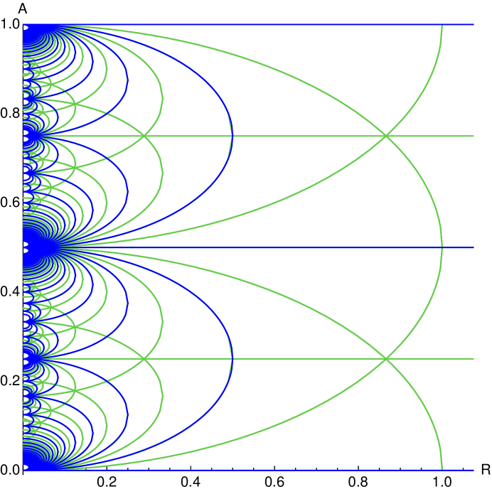
  $$\quad E_{7}\times E_{8}\times U(1)^{2}$$

  $$\quad SU(2)\times E_{7}\times E_{8}\times U(1)$$

  $$\quad E_{8}\times E_{8}\times U(1)$$

$${\fcolorbox{black}{azul}{\rule{0pt}{3pt}\rule{3pt}{0pt}}}+{\fcolorbox{black}{verde}{\rule{0pt}{3pt}\rule{3pt}{0pt}}} \quad SU(2)\times E_{8}\times E_{8}$$

$${\fcolorbox{black}{verde}{\rule{0pt}{3pt}\rule{3pt}{0pt}}}+{\fcolorbox{black}{verde}{\rule{0pt}{3pt}\rule{3pt}{0pt}}}+{\fcolorbox{black}{verde}{\rule{0pt}{3pt}\rule{3pt}{0pt}}} \quad SU(3)\times E_{7}\times E_{8}$$

Figure 25: $\Gamma_{8}\times\Gamma_{8}$ heterotic with Wilson line $A^{I}=\left((A)_{8},0_{8}\right)$

In figure 25 we present these maximal enhancements for the $\Gamma_{8}\times\Gamma_{8}$ theory, and we also show a maximal enhancement to $SU(3)\times E_{7}\times E_{8}$. The additional states with $w=0$ are represented by the cyan line and the states with $|w|=1$ together with the ones with $|w|=2$ are represented by the orange curve.

3.3 Exploring a slice of moduli space

In this section we present a detailed analysis of the slice of moduli space for compactifications of the heterotic theory on a circle at any radius and Wilson line given by

$$A=(A_{1},0_{15})\ .$$ (3.31)

The results of this section are displayed in figure 6. Here we present the main ingredients of the calculations, and leave further details to Appendix C.

For this type of Wilson line, the states with $w=0$ (sector 1) that survive, are those satisfying

$$\pi_{1}A_{1}\in{\mathbb{Z}}\,.$$ (3.32)

This preserves all the roots only if $A_{1}\in\mathbb{Z}$ for the $\Gamma_{16}$ case, or $A_{1}\in 2\mathbb{Z}$ for the $\Gamma_{8}\times\Gamma_{8}$ case. These correspond to the horizontal orange lines in figure 6, where at any generic radius, the gauge symmetry is $U(1)\times SO(32)$, or $U(1)\times E_{8}\times E_{8}$. If $A_{1}$ is an odd number, then the $SO(32)$ symmetry is unbroken, but the $E_{8}\times E_{8}$ is broken to $SO(16)\times E_{8}$, which is depicted with a black line at $A_{1}=1$ in figure 6(b).

If $A_{1}\notin\mathbb{Z}$, then we have just the roots with $\pi_{1}=0$. That is, the $420$ roots of $SO(30)$ or the $324$ roots of $SO(14)\times E_{8}$. This corresponds to the white regions in figure 6.

Now, depending on the value of $R$, we can have additional states in sector 2, i.e. states with non-zero winding which momenta satisfy $|{\bf p_{L}}|^{2}=2$ and have a quantized momentum number on the circle. Then, according to (3.2) and (3.6), they should obey

$$|\pi+wA|^{2}=2(1-w^{2}R^{2})\,,$$ (3.33)

$$\frac{1}{w}\left(1-\tfrac{1}{2}|\pi|^{2}\right)\in\mathbb{Z}\ .$$

The first equation implies $R^{-1}\geq w$, and the simplest solution is

$$\pi=\left(\pm\sqrt{2(1-w^{2}R^{2})}-wA_{1},0_{15}\right)\,.$$

But $\pi$ is in an even lattice, which implies $\pi_{1}=-2q$, $q\in\mathbb{Z}$. The quantization condition for $n$ yields

$$\tfrac{2q^{2}-1}{w}\in\mathbb{Z}\,,$$

so we have only the winding numbers that are divisors of the numbers that can be written as $2q^{2}-1$, for some integer $q$. In terms of $q$, the Wilson lines are of the form

$$A_{1}=\frac{2q\pm\sqrt{2-2w^{2}R^{2}}}{w}\equiv a_{w,q}(R)\ ,\quad\{w,q,\tfrac{2q^{2}-1}{w}\}\in{\mathbb{Z}}\,.$$ (3.34)

If the radius also satisfies $R<\frac{1}{\sqrt{2}w}<\frac{1}{w}$, we have additional solutions where some of the other components of $\pi$ are non-zero, such that

$$\pi+wA= \left(\pm\sqrt{1-2w^{2}R^{2}},\underline{\pm 1,0_{14}}\right)\text{ for $\Gamma_{16}$}\,,$$

$$\pi+wA= \left(\pm\sqrt{1-2w^{2}R^{2}},\underline{\pm 1,0_{6}},0_{8}\right)\text{ for $\Gamma_{8}\times\Gamma_{8}$ }\,.$$

The quantization conditions are the same as before, but now the Wilson lines have the following behavior as a function of the radius

$$A_{1}=\frac{2q+1\pm\sqrt{1-2w^{2}R^{2}}}{w}\equiv b_{w,q}(R)\ ,\quad\{w,q,\tfrac{2q^{2}-1}{w}\}\in{\mathbb{Z}}\,.$$ (3.35)

If additionally $R<(2\sqrt{2}w)^{-1}$ we have yet other possible solutions, but only for the $E_{8}\times E_{8}$ theory, where

$$\pi+wA= \left(\pm\tfrac{1}{2}\sqrt{1-8w^{2}R^{2}},\underline{(\pm\tfrac{1}{2})_{7}},0_{8}\right)\text{ for $\Gamma_{8}\times\Gamma_{8}$. }$$

The lines and quantization conditions are:

$$A_{1}=\frac{q+\tfrac{1}{2}\pm\sqrt{\tfrac{1}{4}-2w^{2}R^{2}}}{w}\equiv c_{w,q}(R)\ ,\quad\{w,q,\tfrac{q(q+1)}{2w}\}\in{\mathbb{Z}}\,,$$ (3.36)

where we used $(\pi_{1})^{2}=|\pi|^{2}-\tfrac{7}{4}$ and $\pi_{1}=-\left(q+\tfrac{1}{2}\right)$.

For a given $q$ and $w$, whenever the Wilson line is of the form $a_{w,q}$ in (3.34), we get $2$ massless states (one for $w>0$ and another one for $w<0$). If there are no more states, then we have enhancement to $U(1)\times SU(2)\times SO(30)$ and $U(1)\times SU(2)\times SO(14)\times E_{8}$. These correspond to the blue lines in figure 6, where for example in figure 6(a), the long blue line going from $(R,A_{1})=(0,\sqrt{2})$ to $(1,0)$ corresponds to $a_{1,0}=\sqrt{2(1-R^{2})}$, while its mirror one along the axis $A_{1}=1$ is $a_{1,1}=2-a_{1,0}$.

For Wilson lines of the form $b_{w,q}$ in (3.35), we get $60$ extra states for the $\Gamma_{16}$, and $28$ for $\Gamma_{8}\times\Gamma_{8}$. The former promote the enhancement to $U(1)\times SO(32)$, while the latter to $U(1)\times SO(16)\times E_{8}$, and they correspond respectively to the orange lines in figure 6(a) and the black lines in figure 6(b). The largest curved orange line in the former and black line in the latter going from $(0,0)$ to $(0,2)$ corresponds to $b_{0,1}=1\pm\sqrt{1-2R^{2}}$, where the plus sign is for the upper half of the curve, and the minus sign for the lower half.

Finally, Wilson lines of the form $c_{w,q}$ in (3.36) give in the $E_{8}\times E_{8}$ heterotic theory, $2\times 2^{6}=128$ states (the sign of one of the seven $(\pm\tfrac{1}{2})$ is determined by the sign of the other $6$ and the sign chosen for the Wilson line). Note that $c_{w,q}(R)=b_{2w,q}(R)$. It is not hard to show that a Wilson line that can be written as $c_{w,q}(R)$ can always be written as $b_{2w,q}(R)$, but the function $b$ can also have an odd $w$. Wilson lines $b$ that can also be written as $c$ bring then a total of $28+128=156$ states, which corresponds to the enhancement to $U(1)\times E_{8}\times E_{8}$ in the orange lines of figure 6(b).

There are only two kinds of intersections between lines, and the points of intersection correspond to points of maximal enhancement (see Appendix C for details):

• between a blue curve $a(R)$ with $w_{1}$ and an orange curve $b(R)$ with $w_{2}$, where the enhancement group is $SU(2)\times SO(32)$ ($SU(2)\times E_{8}\times E_{8})$ in the $SO(32)$ ($E_{8}\times E_{8}$) theory. These are the red dots of figure 6, and arise at

  $$(R,A_{1})=\left(\frac{1}{\sqrt{w_{1}^{2}+2w_{2}^{2}}},\frac{2}{w_{1}}\left(q\pm w_{2}R\right)\right)=\left(\frac{1}{C},\frac{2k}{C}\right)\ ,$$

  for some integer $k$, with $C=1,3,9,11,...$ are all the integers whose prime divisors are 1 or 3 (mod 8) (see Table 3).

• between two blue $a(R)$ with $w_{1}$ and $w_{2}$ and two orange (black) curves $b(R)$ with $w_{3}$ and $w_{4}$, where the enhancement group is $SO(34)$ ($SO(18)\times E_{8}$) for the $SO(32)$ ($E_{8}\times E_{8}$) theory. These are the green dots of figure 6, and arise at

  $$(R,A_{1})=\left(\frac{1}{\sqrt{w_{1}^{2}+w_{2}^{2}}},\frac{2}{w_{1}}\left(q\pm\tfrac{1}{\sqrt{2}}w_{2}R\right)\right)=\left(\frac{1}{\sqrt{2}C},\frac{k}{C}\right)\,,$$

  for some integer $k$, with $C=1,5,13,17,...$ are all the integers whose prime divisors are Pythagorean primes (see Table 3)

In Appendix C we give the details of the calculations and also prove that these are the only possible intersections for this type of Wilson lines. In Appendix D we present other slices of moduli space given by the radius and Wilson lines determined by a single parameter $A$. In section 3.5 we show how these points arise as fixed points of a duality symmetry.

3.4 T-duality in circle compactifications

In this section we discuss the action of T-duality in the heterotic string compactified on a circle. By T-duality we mean the action of certain type of transformations in $O(1,17,{\mathbb{Z}})$ that relate a given heterotic theory with 16-dimensional lattice $\Gamma$, compactified on a circle of radius $R$ and Wilson line $A$, to another heterotic theory with lattice $\Gamma^{\prime}$, compactified on a circle of radius $R^{\prime}$ and Wilson line $A^{\prime}$. In this section we discuss the usual T-duality exchanging momentum and winding numbers, while in the next section we discuss more general dualities, and their fixed points.

The duality generated by the matrix $O_{D}$ is the usual T-duality transformation exchanging momentum and winding numbers

$$(w^{\prime},n^{\prime},\pi^{\prime})=(n,w,\pi)\ .$$ (3.37)

Since $\pi$ stays untouched, this duality is possible if $\Gamma^{\prime}=\Gamma$. Its action on the background fields can be worked out from the generalized metric (2.13), which for the circle is

$${\cal M}=\begin{pmatrix}R^{2}(1+\tfrac{1}{2}{\mathbb{A}}^{2})^{2}&-\tfrac{1}{2}{\mathbb{A}}^{2}&(1+\tfrac{1}{2}{\mathbb{A}}^{2})A\\ -\tfrac{1}{2}{\mathbb{A}}^{2}&\frac{1}{R^{2}}&-\frac{1}{R^{2}}\,A\\ (1+\tfrac{1}{2}{\mathbb{A}}^{2})\,A^{t}&-\frac{1}{R^{2}}\,A^{t}&{\rm I}+\frac{1}{R^{2}}A^{t}A\end{pmatrix}\ ,$$ (3.38)

where we have defined the scalar

$${\mathbb{A}}^{2}\equiv\frac{|A|^{2}}{R^{2}}\ .$$ (3.39)

The action of $O_{D}$ transforms this into

$${\cal M}^{\prime}=O_{D}{\cal M}O^{t}_{D}={\cal M}^{-1}=\begin{pmatrix}\frac{1}{R^{2}}&-\tfrac{1}{2}{\mathbb{A}}^{2}&-\frac{1}{R^{2}}\,A\\ -\tfrac{1}{2}{\mathbb{A}}^{2}&R^{2}(1+\tfrac{1}{2}{\mathbb{A}}^{2})^{2}&(1+\tfrac{1}{2}{\mathbb{A}}^{2})A\\ -\frac{1}{R^{2}}\,A^{t}&(1+\tfrac{1}{2}{\mathbb{A}}^{2})\,A^{t}&{\rm I}+\frac{1}{R^{2}}A^{t}A\end{pmatrix}\,,$$ (3.40)

and thus we get

$$A^{\prime}=-\frac{A}{R^{2}(1+\tfrac{1}{2}{\mathbb{A}}^{2})}\ ,\qquad R^{\prime}=\frac{1}{R\,(1+\tfrac{1}{2}{\mathbb{A}}^{2})}\quad(\,\Rightarrow\,\frac{A^{\prime}}{R^{\prime}}=-\frac{A}{R}\,)\$$

in agreement with the heterotic Buscher rules for scalars [26]. We get that a background has $R^{\prime}=R$ for

$$R_{\rm sd}^{2}=1-\frac{1}{2}|A|^{2}\ \quad(\,\Rightarrow\,R^{\prime}=R\,,\,A^{\prime}=-A\,)$$ (3.41)

Additionally, if $2A\in\Gamma^{\prime}$, then $A^{\prime}=-A\sim A$, and therefore the background is fully self-dual, satisfying ${\cal M}={\cal M}^{-1}$ up to discrete transformations (these are of the form (2.19), (2.20) or (2.21), but for the circle the only non-trivial one is a $\Lambda$-shift (2.21)).

All the examples of enhancement discussed in section 3.2 except for 3.2.8 satisfy the self-duality condition (3.41). By perfoming a $\Lambda$-shift to the Wilson line of 3.2.8 we can bring it to the equivalent one $A=\left((-3/4)_{2},(1/4)_{6},0_{8}\right)$, which satisfies (3.41).

For Wilson lines with only one non-zero component, we have that the fixed “points” of this symmetry correspond actually to lines of non-maximal enhancement symmetry where the Wilson lines are functions of the radius ($A=A(R_{\rm{sd}})$), and are such that $A\sim A_{\rm{sd}}$, with $|A_{\rm{sd}}|^{2}=2(1-R^{2}_{\rm{sd}})$.

We now discuss the differences between fixed points of duality symmetries further, exploring more general dualities and their fixed points.

3.5 More general dualities and fixed points

The transformation $O_{D}$ discussed before is a particular type of transformation that changes the sign of $p_{R}$ while it rotates ${\bf p_{L}}$, preserving its norm (in compactifications of the bosonic theory on a circle, $p_{L}$ has a single component and $O_{D}$ just leaves it invariant, but in the heterotic theory $O_{D}$ rotates the 17-dimensional vector ${\bf p_{L}}$). It would be very interesting to understand what are all the possible transformations that do this, and obtain their fixed points. Here we do something more modest, namely we work out the set of transformations that change the sign of $p_{R}$ and rotate ${\bf p_{L}}$, leaving its circle direction component invariant. We thus require

$$(p_{L}^{\prime},p^{\prime A},p^{\prime}_{R})=(p_{L},U^{AB}p^{B},-p_{R})$$ (3.42)

with $U\in O(16,{\mathbb{Z}})$. These transformations generically link a given heterotic theory with lattice $\Gamma$, in a background defined by $(A,R)$ to another heterotic theory with lattice $\Gamma^{\prime}$ in a dual background with $(A^{\prime},R^{\prime})$. The duality transformation depends on the matrix $U$ and we use a convenient parameterization to relate the radii $R$ and $R^{\prime}$, namely we define a positive number $r$ such that

$$R^{\prime}=\frac{1}{rR}\ .$$ (3.43)

The duality transformation that achieves (3.42) should have the form

$$O_{U}=\begin{pmatrix}-\frac{r|A^{\prime}|^{2}}{2}&\frac{1}{r}+A^{\prime}UA^{t}+\frac{r|A|^{2}}{2}\frac{|A^{\prime}|^{2}}{2}&\frac{r|A^{\prime}|^{2}}{2}A+A^{\prime}U\\ r&-\frac{r|A|^{2}}{2}&-rA\\ -rA^{\prime t}&UA^{t}+\frac{r|A|^{2}}{2}A^{\prime t}&U+rA^{\prime t}A\end{pmatrix}\ .$$ (3.44)

Requiring this to be in $O(1,17;{\mathbb{Z}})$, we get a set of quantization conditions like for example (the full set of quantization conditions is given in (E.2))

$$r\,,\,\frac{r|A|^{2}}{2}\,,\,\frac{r|A^{\prime}|^{2}}{2}\,,\,\frac{1}{r}+A^{\prime}UA+r\frac{|A|^{2}}{2}\frac{|A^{\prime}|^{2}}{2}\in\mathbb{Z}\,.$$ (3.45)

It is instructive to decompose the matrices $O_{U}$ as the product $O_{\Lambda^{\prime}}O_{D}O_{N}O_{M}O_{\Lambda}$ with $\Lambda=-A,M=r$, $N=U$ and $\Lambda^{\prime}=A^{\prime}$, which allows to interpret the transformations as the following series of operations

1. $O_{-A}$: eliminates the Wilson line $A$ through a $\Lambda$-shift,

2. $O_{r}$: rescales $R\rightarrow rR$,

3. $O_{U}$ performs a change of basis in the heterotic directions

4. $O_{D}$: performs a T-duality along the circle ($\eta$),

5. $O_{A^{\prime}}$: adds the Wilson line $A^{\prime}$ through a $\Lambda$-shift.

We divide the discussion into the dualities where $\Gamma=\Gamma^{\prime}$, and those where the dual lattice is not the original one. To denote the different sublattices that will play a role, it is useful to use the $(0)$, $(v)$, $(s)$ and $(c)$ conjugacy classes of $SO(16)$, corresponding respectively to the root, vector, positive and negative-chirality spinor classes. These are defined in (A.4)-(A.7). The lattices $\Gamma_{16}$ and $\Gamma_{8}\times\Gamma_{8}$ contain the following vectors (see (A.10)-(A.11))

$$\Gamma_{16} =(00),(vv),(ss),(cc)$$ (3.46)

$$\Gamma_{8}\times\Gamma_{8} =(00),(ss),(0s),(s0)$$

One could have chosen different conventions in which some of the $s$ classes are turned into $c$ classes, and doing that build four other lattices, that we denote $\Gamma_{16}^{-}$, $\Gamma_{8}^{-}\times\Gamma_{8}^{-}$, $\Gamma_{8}^{-}\times\Gamma_{8}^{+}$ and $\Gamma_{8}^{+}\times\Gamma_{8}^{-}$. We give these in (A.14). Note that a lattice $\Gamma^{+}$ is equivalent to a lattice $\Gamma^{-}$, the choice $(s)$ versus $(c)$ conjugacy class is a convention with no physical relevance. Here it is important however to make the distinction whether a given duality maps, say, $\Gamma^{+}$ to $\Gamma^{+}$, or $\Gamma^{+}$ to $\Gamma^{-}$.

In the following we write the main results, leaving the details to Appendix E. The results for generic Wilson lines, assuming that $r$ is a prime number, are summarized in Table 4. We later concentrate on the situation where the Wilson lines are of the form (3.31), i.e. with only one non-zero component, as we did in section 3.3, to see what happens when the assumption that $r$ is prime is relaxed. For Wilson lines of this form, the $O(16)$ symmetry is broken to $O(15)$, and there are four inequivalent choices of $U$ that we will analyze in detail

$$U=\pm I\ \quad{\rm or}\quad U_{\pm}\equiv\pm\text{diag}(1,-1_{15})\ .$$ (3.47)

3.5.1 $\Gamma\leftrightarrow\Gamma$

The dualities for which the lattice does not change involve those where $\pi$ is invariant, such as the one discussed in the previous section. But as explained above, one can have more general dualities even when $\Gamma^{\prime}=\Gamma$, and thus more general fixed points. Fixed points of a duality are those for which $R^{\prime}=R$ and $A^{\prime}=A$.

To make the analysis tractable for generic Wilson lines, we restrict to the situation where $r$ is a prime number and $U=I$, and relax this assumption only in the setup where the Wilson lines have just one non-zero component. Under the assumption that $r$ is a prime number, the full set of quantization conditions (E.2) are satisfied if and only if (see details in Appendix E)

$$A\in\Gamma\,,\,A^{\prime}\in\Gamma\,,\quad r=1\ ,$$ (3.48)

and thus the fixed points of these transformations are at $R=1$ and $A$ any point in the lattice $\Gamma$. They correspond to enhancements to $SU(2)\times SO(32)$ and $SU(2)\times E_{8}\times E_{8}$ discussed in section 3.1. These points appear in the diagonal entries in Table 4.

Let us now analyze in more detail the fixed points of the dualities for the subset of Wilson lines of the form (3.31), i.e. with only one non-zero component. The quantization conditions evaluated at the fixed points turn into (see Appendix E for details of the calculation)

$$n\,,\,m\,,\frac{2n^{2}\pm 1}{m}\in\mathbb{Z}\quad{\rm for}\quad U=\pm I\quad{\rm where}\ n=\tfrac{1}{2}A_{1}R^{-1},m=R^{-1},$$ (3.49)

and

$$n\,,\,m\,,\frac{n^{2}\pm 1}{2m}\in\mathbb{Z}\quad{\rm for}\quad U=U_{\pm}\quad{\rm where\ now}\ n=\tfrac{1}{\sqrt{2}}A_{1}R^{-1},m=\tfrac{1}{\sqrt{2}}R^{-1}.$$ (3.50)

We write in Table 3 all the fixed points for $U=I$ and $U=U_{+}$ where $0\leq A_{1}\leq 1$. The lines $\pm A_{1}\text{ mod }2$ are also fixed points .

$$\begin{array}{cc}U=\text{diag}(1_{16})& U=\text{diag}(1,-1_{15})\\ & \\ \begin{array}{cc}{R}^{-1}& A_1\\ & \\ 1& 0\\ 3& \frac{2}{3}\\ 9& \frac{4}{9}\\ 11& \frac{8}{11}\\ 17& \frac{10}{17}\\ 19& \frac{6}{19}\\ 27& \frac{22}{27}\\ 33& \frac{8}{33},\frac{14}{33}\\ 41& \frac{30}{41}\\ 43& \frac{16}{43}\\ 51& \frac{10}{51},\frac{44}{51}\\ 57& \frac{32}{57},\frac{44}{57}\\ 59& \frac{36}{59}\\ 67& \frac{20}{67}\\ 73& \frac{12}{73}\\ 81& \frac{22}{81}\\ 83& \frac{74}{83}\\ 89& \frac{40}{89}\\ 97& \frac{80}{97}\\ 99& \frac{14}{99},\frac{58}{99}\end{array}& \begin{array}{cc}{R}^{-1}& A_1\\ & \\ \sqrt{2}& 1\\ 5\sqrt{2}& \frac{3}{5}\\ 13\sqrt{2}& \frac{5}{13}\\ 17\sqrt{2}& \frac{13}{17}\\ 25\sqrt{2}& \frac{7}{25}\\ 29\sqrt{2}& \frac{17}{29}\\ 37\sqrt{2}& \frac{31}{37}\\ 41\sqrt{2}& \frac{9}{41}\\ 53\sqrt{2}& \frac{23}{53}\\ 61\sqrt{2}& \frac{11}{61}\\ 65\sqrt{2}& \frac{47}{65},\frac{57}{65}\\ 73\sqrt{2}& \frac{27}{73}\\ 85\sqrt{2}& \frac{13}{85},\frac{47}{85}\\ 89\sqrt{2}& \frac{55}{89}\\ 97\sqrt{2}& \frac{75}{97}\\ 101\sqrt{2}& \frac{91}{101}\\ 109\sqrt{2}& \frac{33}{109}\\ 113\sqrt{2}& \frac{15}{113}\\ 125\sqrt{2}& \frac{57}{125}\\ 137\sqrt{2}& \frac{37}{137}\\ 145\sqrt{2}& \frac{17}{145},\frac{133}{145}\end{array}\\ & \\ SU(2)\times SO(32)& SO(34)\\ \mathrm{or}& \mathrm{or}\\ SU(2)\times E_8\times E_8& SO(18)\times E_8\end{array}$$

Table 3: Fixed points of the dualities $O_{U}$.

These points in moduli space are points of maximal enhancement symmetry. Those in the first column give rise to $SU(2)\times SO(32)$ for $\Gamma_{16}$ or $SU(2)\times E_{8}\times E_{8}$ for $\Gamma_{8}\times\Gamma_{8}$, and are depicted by red dots in figure 6. The second column contains all the points of maximal enhancement groups $SO(34)$ or $SO(18)\times E_{8}$, and correspond to the green dots in figure 6.

3.5.2 $\Gamma\leftrightarrow\Gamma^{\prime}$

Note that unless $\Gamma=\Gamma_{16}^{\pm}$ and $\Gamma^{\prime}=\Gamma_{8}^{\pm}\times\Gamma_{8}^{\pm}$ (or the other way around, and using any combination of signs) $-$ situations that we analyze separately in the next section $-$ there exists some $U_{1}\in O(16,{\mathbb{Z}})$ such that $\Gamma^{\prime}=U_{1}\Gamma$. In that case, the duality with $\Gamma^{\prime}\neq\Gamma$, $U_{2}$ and $A^{\prime}$ is equivalent to one between $\Gamma$ and $\Gamma^{\prime\prime}=\Gamma$, $U^{\prime\prime}=U_{1}U_{2}$ and has $A^{\prime\prime}=A^{\prime}U_{1}$. Restricting to diagonal matrices $U$, we see that the dualities with $U$ and $\Gamma^{\prime}=\Gamma$ are equivalent to the dualities with $U=I$ but where $\Gamma^{\prime}$ is

$$\Gamma^{\prime}=\Gamma^{\pm}_{16}\text{ for }\Gamma=\Gamma_{16}\text{ and det}(U)=\pm 1$$ (3.51)

$$\Gamma^{\prime}=\Gamma^{\pm_{1}}_{8}\times\Gamma^{\pm_{2}}_{8}\text{ for }\Gamma=\Gamma_{8}\times\Gamma_{8},\text{ det}_{1}(U)=\pm_{1}1\text{ and det}_{2}(U)=\pm_{2}1$$ (3.52)

where $\text{det}_{1}$ ($\text{det}_{2}$) is the product of the $8$ first (last) diagonal elements and the lattices $\Gamma^{\pm}$ are defined in Appendix A. If additionally the Wilson line $A$ is invariant under the action of $U$ (up to a $\Lambda$-shift) we get exactly the same fixed points that one gets for a duality with $\Gamma=\Gamma^{\prime}$. Since Wilson lines of the type (3.31) are invariant under the action of a diagonal $U$ such that the first component is +1, we get the same fixed points of section 3.5.1 that correspond to enhancement to $SO(34)$ or $SO(18)\times E_{8}$.

Under the assumption that $r$ is a prime number, the quantization conditions are satisfied if and only if

$$A\in(\Gamma\cap \Gamma^{\prime})^{*}\backslash\Gamma\,,\,A^{\prime}\in(\Gamma\cap\Gamma^{\prime})^{*}\backslash\Gamma^{\prime}\,,\,r=2$$ (3.53)

and thus the fixed points of these transformations are at $R=\tfrac{1}{\sqrt{2}}$, and correspond to the enhancements $SO(34)$ and $SO(18)\times E_{8}$. The possible Wilson lines for the different choices of $\Gamma$ and $\Gamma^{\prime}$ are given in Table 4.

3.5.3 $SO(32)\leftrightarrow E_{8}\times E_{8}$

There is no $U\in O(16,{\mathbb{Z}})$ that transforms the lattices $\Gamma_{16}$ and $\Gamma_{8}\times\Gamma_{8}$ into each other, and thus the case $\Gamma=\Gamma_{16}$ and $\Gamma^{\prime}=\Gamma_{8}\times\Gamma_{8}$ is different from the ones considered previously.

Here, for simplicity, we restrict to $U=1$, namely we analyze dualities such that $({\bf p_{L}}^{\prime},p^{\prime}_{R})=({\bf p_{L}},-p_{R})$. The quantization conditions under the assumption that $r$ is a prime number, are given in (3.53). For $\Gamma=\Gamma_{16}$ and $\Gamma^{\prime}=\Gamma_{8}\times\Gamma_{8}$, the possible Wilson lines are the following

$$A\in(\Gamma\cap\Gamma^{\prime})^{*}\backslash\Gamma=(0s),(s0),(vc),(cv)$$ (3.54)

$$A^{\prime}\in(\Gamma\cap\Gamma^{\prime})^{*}\backslash\Gamma^{\prime}=(vv),(cc),(vc),(cv)$$

However, there is something very curious here: the fixed points of these dualities, corresponding to $R=\frac{1}{\sqrt{2}}$, are not points of maximal enhancement but points of enhancement $U(1)\times SO(16)\times SO(16)$. Furthermore, this enhancement group arises at any radius, so Wilson lines of the form (3.54) give rise to lines in moduli space, and as such are also “fixed points” of dualities that do not involve $O_{D}$.

Let us illustrate this better with an example: Take $A=((\frac{1}{2})_{8},0_{8})\in(s0)$ and $A^{\prime}=(1,0_{7},1,0_{7})\in(vv)$. For the time being, we take $r=2$, i.e. $R^{\prime}=1/(2R)$, but we do not necessarily stand at the self-dual radius.

The Wilson line $A$ breaks the $SO(32)$ gauge symmetry to $SO(16)\times SO(16)$, as shown in section 3.2.3. For this Wilson line, one has additionally states which are neutral under $SO(16)\times SO(16)$, i.e. with $p^{A}=0$. Since these should have $\pi=-wA$, then only states with $w=2m$, $m\in\mathbb{Z}$ are allowed. These states have left and right-moving momenta on the circle

$$p_{L}=\frac{1}{\sqrt{2}R}\left(\tilde{n}+2R^{2}m\right)\,,\qquad p_{R}=\frac{1}{\sqrt{2}R}\left(\tilde{n}-2R^{2}m\right)\,,$$ (3.55)

where $\tilde{n}=n+w$. Let us pause for a second to show that there is no enhacement to $SU(2)\times SO(16)\times SO(16)$ with this Wilson line. We have shown in section 3.2.3 that there are no additional massless states charged under $SO(16)\times SO(16)$, i.e. with non-zero winding number and $p^{A}\neq 0$. Regarding extra neutral massless states, it is very easy to see from (3.55) that there are none of this form: states with momenta $(p_{L},p^{A},p_{R})=(\sqrt{2},0,0)$, satisfy $2R^{2}m=\tilde{n}$, while requiring at the same time $p_{L}=\sqrt{2}$ would lead to $\tilde{n}m=\tfrac{1}{2}$, which has no solution. Thus, the compactification of the $SO(32)$ heterotic string with Wilson line $A=((\frac{1}{2})_{8},0_{8})$ leads to $U(1)\times SO(16)\times SO(16)$ at any radius.

The Wilson line $A^{\prime}=(1,0_{7},1,0_{7})$ breaks the $E_{8}\times E_{8}$ symmetry also to $SO(16)\times SO(16)$. There are also states which are neutral under $SO(16)\times SO(16)$, of the same form as before, i.e. with momenta

$$p^{\prime}_{L}=\frac{1}{\sqrt{2}R^{\prime}}\left(\tilde{n}^{\prime}+2R^{\prime 2}m^{\prime}\right)\,,\qquad p^{\prime}_{R}=\frac{1}{\sqrt{2}R^{\prime}}\left(\tilde{n}^{\prime}-2R^{\prime 2}m^{\prime}\right)\,,$$ (3.56)

where $w^{\prime}=2m^{\prime}$ and $\tilde{n}^{\prime}=n^{\prime}+w^{\prime}$.

Comparing (3.56) and (3.55), we see that $(p^{\prime}_{L},p_{R})=(p_{L},-p_{R})$ if $(\tilde{n}^{\prime},m^{\prime})=(m,\tilde{n})$ and $RR^{\prime}=\frac{1}{2}$. This is true for any value of $R$.

In the following table we write the fixed points of the dualities between a theory with lattice $\Gamma$ (row) and another one with $\Gamma^{\prime}$ (column) for the smallest value of the parameter $r$ defined in (3.43), which are $r=1$ or $r=2$. We indicate the conjugation classes of the possible Wilson lines (for a given row and column, any $A$ given can be dualized to any $A^{\prime}$), and the enhancement group arising at the fixed point of the duality.

	$\Gamma_{16}$	$\Gamma^{-}_{16}$	$\Gamma_{8}\times\Gamma_{8}$	$\Gamma_{8}\times\Gamma^{-}_{8}$	$\Gamma^{-}_{8}\times\Gamma_{8}$	$\Gamma^{-}_{8}\times\Gamma^{-}_{8}$
$\Gamma_{16}$	$SO(32)\times SU(2)$	$SO(34)$	$SO(16)\times SO(16)\times U(1)$	-	-	$SO(16)\times SO(16)\times U(1)$
	$R=1$	$R=1/\sqrt{2}$	$R=1/\sqrt{2}$			$R=1/\sqrt{2}$
	$A=00,ss,vv,cc$	$A=0v,v0,cs,sc$	$A=vc,cv,0s,s0$			$A=vs,sv,0c,c0$
	$A^{\prime}=00,ss,vv,cc$	$A^{\prime}=0v,v0,ss,cc$	$A^{\prime}=vc,cv,vv,cc$			$A^{\prime}=vs,sv,vv,ss$
$\Gamma^{-}_{16}$		$SO(32)\times SU(2)$	-	$SO(16)\times SO(16)\times U(1)$	$SO(16)\times SO(16)\times U(1)$	-
		$R=1$		$R=1/\sqrt{2}$	$R=1/\sqrt{2}$
		$A=00,ss,sc,cs$		$A=vs,cv,s0,0c$	$A=sv,vc,0s,c0$
		$A^{\prime}=00,ss,sc,cs$		$A^{\prime}=vs,cv,cs,vv$	$A^{\prime}=sv,vc,sc,vv$
$\Gamma_{8}\times\Gamma_{8}$			$E_{8}\times E_{8}\times SU(2)$	$E_{8}\times SO(18)$	$SO(18)\times E_{8}$	-
			$R=1$	$R=1/\sqrt{2}$	$R=1/\sqrt{2}$
			$A=00,ss,0s,s0$	$A=0v,sv,0c,sc$	$A=v0,vs,c0,cs$
			$A^{\prime}=00,ss,0s,s0$	$A^{\prime}=0v,sv,0s,ss$	$A^{\prime}=v0,vs,s0,ss$
$\Gamma_{8}\times\Gamma^{-}_{8}$				$E_{8}\times{E_{8}}^{-}\times SU(2)$	-	$SO(18)\times{E_{8}}^{-}$
				$R=1$		$R=1/\sqrt{2}$
				$A=00,sc,0c,s0$		$A=v0,vc,c0,cc$
				$A^{\prime}=00,sc,0c,s0$		$A^{\prime}=v0,vc,s0,sc$
$\Gamma^{-}_{8}\times\Gamma_{8}$					${E_{8}}^{-}\times E_{8}\times SU(2)$	${E_{8}}^{-}\times SO(18)$
					$R=1$	$R=1/\sqrt{2}$
					$A=00,cs,0s,c0$	$A=0v,cv,0c,cc$
					$A^{\prime}=00,cs,0s,c0$	$A^{\prime}=0v,cv,0s,cs$
$\Gamma^{-}_{8}\times\Gamma^{-}_{8}$						${E_{8}}^{-}\times{E_{8}}^{-}\times SU(2)$
						$R=1$
						$A=00,cc,0c,c0$
						$A^{\prime}=00,cc,0c,c0$

Table 4: Points of symmetry enhancement as fixed points of duality symmetries

4 Effective action and Higgs mechanism

Now that we saw the rich structure of duality symmetry, we turn to its explicit target space realization. The global duality symmetry of the dimensionally reduced heterotic supergravity action has been deeply investigated in the seminal papers by J. Maharana and J. Schwarz [6] and N. Kaloper and R. Myers [7], and more recently in [8]. If the gauge fields are truncated to the Cartan subsector of the $E_{8}\times E_{8}$ or $SO(32)$ gauge group, the dimensional reduction of heterotic supergravity from 10 to $10-k$ dimensions produces a theory with $U(1)^{2k+16}$ abelian gauge symmetry and a continuous global $O(k,k+16;\mathbb{R})$ symmetry. If the reduction includes the full set of $E_{8}\times E_{8}$ or $SO(32)$ gauge fields and no Wilson lines, the global symmetry reduces to $O(k,k;\mathbb{R})$, while a compactification with Wilson lines for the Cartan gauge fields of a rank $16-r$ subgroup of the rank 16 gauge group $G_{L}$, gives an effective field theory with global $O(k,k+16-r;\mathbb{R})$ duality symmetry [8]. The analysis of [8] is based on string-theoretic arguments and holds to any order in the $\alpha^{\prime}$ expansion of the heterotic string effective field theory action involving all the massless string states, except those that become massless at self-dual points of the moduli space.

Including the massless states with nonzero winding or momentum number on $T^{k}$ in the effective field theory of the toroidally compactified heterotic string is not difficult, as it is a gauged supergravity. The action with at most two derivatives of the massless fields is then completely determined by the gauge group. Therefore, although the field theoretical Kaluza-Klein reduction of heterotic supergravity cannot describe the string modes that give rise to maximally enhanced gauge symmetry, the action is entirely fixed.

Nevertheless, we will see in the forthcoming sections that the explicit construction of the (toroidally compactified) heterotic string effective action from the scattering amplitudes of massless string modes at self dual points of the moduli space, and its manifestly duality-covariant reformulation, give important information. In particular, we will obtain novel relations between the $SO(32)$ and $E_{8}\times E_{8}$ theories. We will also consider the light states that acquire mass when slightly perturbing the background fields and revisit the gauge symmetry breaking and Higgs mechanism, both from the field theory and the string theory viewpoints.

4.1 Effective action of massless states

The three-point functions of all the (toroidally compactified) heterotic string massless vertex operators are reviewed in Appendix F, where we also compute the four point function of the massless scalars. These amplitudes are reproduced from the S-matrix of the following effective action

$$S = \frac{1}{{2\kappa_{d}^{2}}}\int d^{d}x{\sqrt{-G}}e^{-2{\varphi}}\left({R}+4\partial_{\mu}\varphi\partial^{\mu}\varphi-\frac{1}{12}H_{\mu\nu\rho}H^{\mu\nu\rho}-\frac{1}{4}F_{\mu\nu}^{\Gamma}F^{\mu\nu}_{\Gamma}-\frac{1}{4}\bar{F}_{\mu\nu}^{m}\bar{F}^{\mu\nu}_{m}\right.$$ (4.1)

$$\ \ \ \ \ \ \ -\frac{1}{4}D_{\mu}{\rm S}^{mn}D^{\mu}{\rm S}_{mn}-\frac{1}{{2}}{S}_{\Gamma m}F^{\Gamma}_{\mu\nu}\bar{F}^{m\mu\nu}-\ \frac{1}{4}\ {\rm S}_{\Gamma m}{\rm S}_{\Gamma^{\prime}}{}^{m}{\rm S}_{\Lambda n}{\rm S}_{\Lambda^{\prime}}{}^{n}f^{\Gamma\Lambda\Pi}f^{\Gamma^{\prime}\Lambda^{\prime}}{}_{\Pi}\Bigg{)},\ \ \ \ \$$

which also contains terms from higher point functions that we have not computed but need to be included on the basis of gauge symmetry. Here $\kappa_{d}$ is the effective Planck coupling constant (related to the gauge coupling $g_{d}$ as $g_{d}=\sqrt{2}\kappa_{d}$) and

$$H_{\mu\nu\rho} = 3\left(\partial_{[\mu}B_{\nu\rho]}+A^{\Gamma}_{[\mu}\partial_{\nu}A_{\rho]\Gamma}+\frac{1}{3}f_{\Gamma\Lambda\Omega}A_{\mu}^{\Gamma}A_{\nu}^{\Lambda}A_{\rho}^{\Omega}-\bar{A}^{m}_{[\mu}\partial_{\nu}\bar{A}_{\rho]m}\right)\,,$$ (4.2)

$$F_{\mu\nu}^{\Gamma} = \partial_{\mu}A_{\nu}^{\Gamma}-\partial_{\nu}A_{\mu}^{\Gamma}+f^{\Gamma}{}_{\Lambda\Omega}A_{\mu}^{\Lambda}A_{\nu}^{\Omega}\,,\quad\bar{F}_{\mu\nu}^{m}=\partial_{\mu}\bar{A}_{\nu}^{m}-\partial_{\nu}\bar{A}_{\mu}^{m}\,,$$

$$D_{\mu}{\rm S}^{\Gamma m} = \partial_{\mu}{\rm S}^{\Gamma m}+f^{\Gamma}{}_{\Lambda\Omega}A_{\mu}^{\Lambda}{\rm S}^{\Omega m}\,,$$ (4.3)

with ${\rm S}_{\Gamma m}=({\rm G}_{mn},{\rm B}_{mn},{\rm A}_{Im},{\rm A}_{\alpha m})$ denoting the scalar fields. The indices $m,n=1,\dots,k$ correspond to the dimensions on $T^{k}$ and $\Gamma,\Lambda=1,...,N$ are the adjoint indices of the Lie algebra associated to the gauge group $G_{L}$ of dimension $N$ and structure constants $f^{\Gamma}{}_{\Lambda\Omega}$.

For ten external dimensions (i.e. when there are no compact internal dimensions other than the 16 chiral “heterotic” ones), $d=10$, the gauge group is $E_{8}\times E_{8}$ or $SO(32)$ and $N=496$. There are neither scalar ${\rm S}_{\Gamma m}$ nor vector $A_{\mu}^{m},\bar{A}_{\mu}^{m}$ fields. Then the action reduces to the first four terms in (4.1), with $\Gamma=(I,\alpha)=1,\dots,496$, and the last term in $H_{\mu\nu\rho}$ vanishes.

For compactifications on $T^{k}$, $d=10-k$, at generic values of the background fields, the gauge group is $U(1)^{16+k}_{L}\times U(1)_{R}^{k}$, $N=16+k$, and the index $\Gamma\equiv\hat{I}=1,\dots,16+k$. The vectors and scalars are only those in sector 1 of section 2.3. We denote the gauge fields as the polarization vectors in the vertex operators $(A_{\mu}^{m},A_{\mu}^{I},\bar{A}_{\mu}^{m})$ and the scalar fields are ${\rm G}_{mn}={G}_{mn}+{S_{(mn)}(x)}$, ${\rm B}_{mn}=B_{mn}+{S_{[mn]}(x)}$, ${\rm A}_{Im}=A_{Im}+{S_{Im}(x)}$, where the fluctuations are denoted like the polarizations of the vertex operators creating the string scalar states. In this case, (4.1) agrees with the effective action obtained in [6] from dimensional reduction of heterotic supergravity with gauge group truncated to the Cartan subgroup. The theory has a global $O(k,k+16;\mathbb{R})$ symmetry.

At the specific points in moduli space where the gauge symmetry is enhanced, it is convenient to split the index $\Gamma=({\hat{I},\alpha=\overline{\alpha},\underline{\alpha}})$, where $\hat{I}=1,...,16+k$ denotes the Cartan generators and $\underline{\alpha}$ $(\overline{\alpha})$ are the positive (negative) roots of $G_{L}$. The vectors $A_{\mu}^{\hat{I}}$ and $\bar{A}_{\mu}^{m}$ correspond to the left and right Cartan generators in sector 1, respectively, while $A_{\mu}^{\alpha}$ correspond to the vectors of sector 2, as defined in section 2.3. The scalars ${\rm S}^{\hat{I}m}$ correspond to the $(16+k)\times k$ scalars in sector 1, while the ${\rm S}^{\alpha m}$ correspond to the scalars in sector 2. In this case, ${\rm G}_{mn}={G}^{sd}_{mn}+{S_{(mn)}(x)}$, ${\rm B}_{mn}=B^{sd}_{mn}+{S_{[mn]}(x)}$, ${\rm A}_{Im}=A^{sd}_{Im}+{S_{Im}(x)},{\rm A}_{\alpha m}={S_{\alpha m}(x)}$, and the superindex $sd$ refers to the self-dual values of the background fields. The algebra in the Cartan-Weyl basis is

$$\left[J^{\hat{I}},J^{\alpha}\right]=\alpha^{\hat{I}}J^{\alpha}\,,\ \ \ \ \left[J^{\alpha},J^{\beta}\right]=\left\{\begin{matrix}\varepsilon({\bf{\alpha,\beta}})J^{\alpha+\beta}&{\rm if}\ {\bf\alpha}+{\bf\beta}\ {\rm is\ a\ root}\\ {\alpha}_{\hat{I}}\ J^{\hat{I}}&{\rm if}\ {\bf\alpha}=-{\bf\beta}\\ 0&{\rm otherwise}\end{matrix}\right.\,,$$

where $\varepsilon(\alpha,\beta)=\pm 1$ for simply-laced algebras. Note that it is completely determined by the vertex operators of the vector states: the roots $\alpha^{\hat{I}}$ are the momenta of the string states and $\varepsilon(\alpha,\beta)$ is given by the cocycle factors in the currents (2.42) $c_{\alpha}c_{\beta}=\varepsilon(\alpha,\beta)c_{\alpha+\beta}$. When the gauge group $G_{L}$ is a product, the structure constants (and the indices $\Gamma,\hat{I},\alpha)$ split into those of each factor, e.g. for $SO(32)\times H$, $\Gamma=(\Gamma_{SO(32)},\Gamma_{H})$ with $\Gamma_{SO(32)}=(I=1,\dots,16;\alpha=1,\dots,480)$ and $\Gamma_{H}=(m=1,\dots,k;\alpha=1,\dots,N-496-k)$, while for $SO(32)\times U(1)_{L}^{k}$ or $SO(34)$ they are only those of the non-Abelian piece. The Cartan-Killing metric is defined to be a block diagonal matrix containing the Cartan-Killing metrics of the groups $\kappa={\rm diag}(\kappa_{SO(32)},\kappa_{H})$ or $\kappa={\rm diag}(\kappa_{SO(32)},1_{k\times k})$.

For gauge groups of the form $G_{L}\times U(1)_{L}^{k}\times U(1)_{R}^{k}$, the action (4.1) agrees with the dimensionally reduced heterotic supergravity action obtained in [8], including the scalar potential (although the reduction of [8] contains an additional term with six scalars that we have not computed). It possesses $O(k,k;\mathbb{R})$ global symmetry.

In the case of enhanced gauge groups of the form $G_{L}\times U(1)_{R}^{k}$, in which the $k$ left-moving Cartan generators are absorbed by the Cartan subgroups of the non-abelian group $G_{L}$, the structure constants completely break the global symmetry. However, (4.1) can be rewritten in $O(k,n)$ covariant form, where $n$ equals the dimension of the full gauge group. We review this rewriting in the next section, where we also present an alternative reformulation of (4.1) from a generalized Scherk-Schwarz compactification of double field theory. This will allow us to obtain novel relations between the $E_{8}\times E_{8}$ and $SO(32)$ heterotic theories.

From (4.1) one can see some of the features of the spontaneous breaking of gauge symmetry that occurs away from the enhancement points. An effective stringy Higgs mechanism is already encoded in the string theory computation, which can be interpreted as triggered by the vacuum expectation values of the scalar fields in the Cartan sector ${\rm S}_{\hat{I}m}$, which give mass to the vectors in the non-Cartan sector from the covariant derivatives in the kinetic terms, while the scalars without legs in the Cartan sector acquire mass from the scalar potential. We present the relevant details in the forthcoming sections.

4.2 Higgs mechanism in string theory

When moving away from the points in moduli space where the gauge symmetry is enhanced, ${\bf p_{R}}\neq 0$ and the extra massless vectors and scalars in sector 2 acquire mass. The dependence of the vertex operators on the background fields is contained in the exponential factors of the internal coordinates, which become

$$J^{\alpha}=c_{\alpha}e^{i\pi_{(\alpha)\hat{I}}Y_{L}^{\hat{I}}(z)}\rightarrow J^{p_{L},p_{R}}(z,\bar{z})=c^{\prime}_{\alpha}e^{ip_{L\hat{I}}Y_{L}^{\hat{I}}(z)+ip_{Rm}Y_{R}^{m}(\bar{z})}\,,$$ (4.4)

where $c^{\prime}_{\alpha}=c_{\alpha}$, as we will see later. In particular, the $[U(1)_{L}]^{k+16}\times[U(1)_{R}]^{k}$ charges of these states, $(q^{\hat{I}},\bar{q}^{m})=(p_{L}^{\hat{I}},p_{R}^{m})$, are generated by $J^{\hat{I}}\otimes J^{m}$.

The OPE of the energy-momentum tensor with the massive vector boson vertex operators develop a cubic pole, and it is necessary to combine these operators with those of the massive scalars in order to cancel the anomaly. As discussed in [12], the vertex operators of the massless vectors “eat” the scalars $S^{\alpha m}$ and the conformal anomalies can be canceled when redefining

$$A_{(0)}^{\prime}\sim J^{p_{L},p_{R}}(z,\bar{z})\left(A^{\alpha}_{\mu}(k)\bar{\Upsilon}^{\prime\mu}(\bar{z})-\xi S^{\alpha m}(k)\bar{\Upsilon}^{\prime}_{m}(\bar{z})\right)e^{ik\cdot X(z,\bar{z})}\,,$$ (4.5)

with

$${\bar{\Upsilon}}^{\prime\mu}=i\sqrt{2}\bar{\partial}X^{\mu}+\frac{1}{\sqrt{2}}k\cdot\bar{\psi}\bar{\psi}^{\mu}-p_{Rn}\bar{\chi}^{n}\bar{\psi}^{\mu}\,,\qquad{\bar{\Upsilon}}^{\prime m}=i\bar{\partial}Y^{m}+\frac{1}{\sqrt{2}}k\cdot\bar{\psi}\bar{\chi}^{m}-p_{Rn}\bar{\chi}^{n}\bar{\chi}^{m}\,,$$

if

$$k\cdot A_{\alpha}-\xi p^{m}_{R}S_{\alpha m}=0\,,$$ (4.6)

where $\xi$ is some coefficient. In terms of fields, this is

$$\partial_{\mu}A_{\alpha}^{\mu}+i\xi p_{R}^{m}S_{\alpha m}=0\,,$$ (4.7)

corresponding to the $R_{\xi}$ t’Hooft gauge condition where $p_{R}$ can be identified with a non vanishing vev. Then the physical massive vector boson vertices are actually $A^{\prime}$, and the scalars $S_{\alpha m}$ disappear from the spectrum.

Note that the fields associated to $A^{\prime}$ have well defined charges $(\bf{p_{L}},\bf{p_{R}})$, and since $m^{2}=-k^{2}$, the gauge condition can be written as

$$k\cdot\left(A_{\alpha}+k\xi\frac{1}{2p_{R}^{2}}p_{R}^{m}S_{\alpha m}\right)=0\,,$$ (4.8)

implying an effective polarization

$$A^{\prime}_{\alpha\mu}(p_{L},p_{R},k)=A_{\alpha\mu}-\xi\frac{k_{\mu}}{2p_{R}^{2}}p_{R}^{m}S_{\alpha m}\,.$$ (4.9)

This leads to a massive vector of the form

$$A^{\prime}_{\alpha\mu}=A_{\alpha\mu}-\xi\frac{1}{2p_{R}^{2}}p_{R}^{m}\partial_{\mu}S_{\alpha m}\,,$$ (4.10)

where $p_{R}^{2}\neq 0$ is related to the vevs. This is the usual massive vector field incorporating the would-be Goldstone bosons $p_{R}^{m}S_{\alpha m}$ that provide the longitudinal polarization.

Unlike the case of the toroidally compactified bosonic string, in the heterotic string all the massive scalars are Goldstone bosons. Since the gauge group in the supersymmetric right sector is abelian, there are no other massive scalars from the compactification of the massless states.

The non-vanishing three point functions involving massless and light states, i.e. states that are massless at the self-dual points and become massive when perturbing the background fields, are listed in Appendix C, and they lead to the following effective action

$$S^{\prime} = \frac{1}{2\kappa_{d}^{2}}\int d^{d}x{\sqrt{G}}{e^{-2\varphi}}\Big{(}{R}+4(\partial_{\mu}\varphi)^{2}-\frac{1}{12}H^{\prime}_{\mu\nu\rho}H^{\prime\mu\nu\rho}-\frac{1}{4}F_{\mu\nu}^{\hat{I}}F^{\mu\nu}_{\hat{I}}-\frac{1}{4}\bar{F}_{\mu\nu}^{m}\bar{F}^{\mu\nu}_{m}$$ (4.11)

$$\ \ \ \ \ \ \ \ -\frac{1}{4}{F^{\prime}}_{\mu\nu}^{p}F^{{}^{\prime}-p\mu\nu}-\frac{1}{2}p_{R}^{2}A^{\prime p}_{\mu}A^{\prime-p}_{\nu}G^{\mu\nu}-\frac{1}{4}\partial_{\mu}{\rm S}_{\hat{I}n}\partial^{\mu}{\rm S}^{\hat{I}n}+\sqrt{2}p_{L}^{\hat{I}}p_{R}^{m}A^{\prime p\mu}A^{\prime}_{p\mu}S_{\hat{I}m}$$

$$\ \ \ \ \ \ \ \ \left.-\frac{1}{{2}}F^{\hat{I}}_{\mu\nu}\bar{F}^{m\mu\nu}S_{\hat{I}m}+\frac{i}{2}p_{L}^{\hat{I}}A^{\prime p}_{\mu}A^{\prime-p}_{\nu}F^{\mu\nu}_{\hat{I}}-\frac{i}{2}p_{R}^{m}A^{\prime p}_{\mu}A^{\prime-p}_{\nu}\bar{F}_{\mu\nu}^{m}\right)$$

with

$$F^{\prime p_{1}}_{\mu\nu} = 2\partial_{[\mu}A^{\prime p_{1}}_{\nu]}+\varepsilon(p_{1},p_{2})A^{\prime-p_{2}}_{[\mu}A^{\prime p_{1}+p_{2}}_{\nu]}-2i{p_{1L}}_{\hat{I}}A_{[\mu}^{\hat{I}}A^{\prime p_{1}}_{\nu]}-2i{p_{1R}}_{m}\bar{A}_{[\mu}^{m}A^{\prime p_{1}}_{\nu]}$$

$$F_{\mu\nu}^{\hat{I}} = 2\partial_{[\mu}A_{\nu]}^{\hat{I}}\,,\qquad\bar{F}_{\mu\nu}^{m}=2\partial_{[\mu}\bar{A}_{\nu]}^{m}$$

$$H^{\prime}_{\mu\nu\rho} = 3\left(\partial_{[\mu}B_{\nu\rho]}+A^{\hat{I}}_{[\mu}\partial_{\nu}A_{\rho]\hat{I}}+A^{\prime p}_{[\mu}\partial_{\nu}A^{\prime}_{\rho]p}+\frac{1}{3}\varepsilon(p_{1},p_{2})A^{\prime p_{1}}_{\mu}A^{\prime p_{2}}_{\nu}A^{\prime-p_{1}-p_{2}}_{\rho}\right.$$ (4.12)

$$\left.\ \ \ \ \ \ \ \ \ \ \ \ \ -i\ p_{L\hat{I}}A^{\prime p}_{[\mu}A^{\prime-p}_{\nu}A_{\rho]}^{\hat{I}}-ip_{Rm}A^{\prime p}_{[\mu}A^{\prime-p}_{\nu}A_{\rho]}^{m}-\bar{A}^{m}_{[\mu}\partial_{\nu}\bar{A}_{\rho]m}\right)\,,$$

The S-matrix of this massive gauge field theory coupled to gravity reproduces the string theory three-point amplitudes. The non-Abelian pieces in the field strength of the massive gauge fields and in the Chern-Simons terms in $H^{\prime}_{\mu\nu\rho}$ correctly appear in terms of the charges of the corresponding fields $(q^{\hat{I}},q^{m})=(p^{\hat{I}}_{L},p^{m}_{R})$. These charges determine the coefficients of the vector boson three-point functions, which can be identified with structure constants

$$f^{m}{}_{\underline{p}\ \overline{p}}=ip_{R}^{m}\,,\qquad f^{\hat{I}}{}_{\underline{p}\ \overline{p}}=ip_{L}^{\hat{I}}\,,\qquad f^{p_{1}+p_{2}}{}_{p_{1}p_{2}}=\varepsilon(p_{1},p_{2})\,,$$ (4.13)

reflecting the fact that the gauge interactions in string theory are a manifestation of an underlying affine Lie algebra. This algebra is isomorphic to that of the enhanced $G_{L}$ group [15], which justifies the identification $c^{\prime}_{\alpha}=c_{\alpha}$ used in (4.4) (we will comment further on this result in the next section).

Not all the terms in the action can be obtained from the three-point functions, but we have completed the expressions so that they correctly reproduce the massless case when $p_{R}=0$ and $p_{L}\in\Gamma$.

All the terms of the scalar potential of the massless theory (4.1) are absorbed by the field strengths of the massive vectors or by interaction terms containing massive vectors.

5 Heterotic double field theory

Although the action (4.1) can be generically obtained by dimensional reduction of heterotic supergravity from 10 to $10-k$ dimensions, not all the effective actions of massless fields obtained from toroidally compactified heterotic string theory can be uplifted to higher dimensional supergravities. In particular, the states with nonzero winding or momentum number on $T^{k}$ cannot be captured by field theoretical Kaluza Klein compactifications. To find the higher dimensional description of these string modes, one has to refer to gauged double field theory (DFT) [23, 24, 27], an $O(D,D+N;\mathbb{R})$ covariant rewriting of heterotic supergravity, with $D$ the dimension of space-time and $N$ the dimension of the gauge group.

In this section we review this construction and show that the effective action (4.1) can be rewritten in terms of $O(k,N)$ multiplets. The reformulation is achieved essentially assembling the $N+k$ gauge fields as a vector, the $Nk$ moduli scalars as part of a symmetric tensor and the structure constants of the non-abelian gauge groups as an antisymmetric three-index tensor under $O(k,N)$ transformations. The procedure generalizes the analysis of [8] by including all the massless string modes at self-dual points of the moduli space, in which the $k$ left Kaluza-Klein vector fields become part of the Cartan subgroup of the maximally enhanced gauge group.

Furthermore, using the equivalence between gauged DFT and generalized Scherk-Schwarz (gSS) compactifications [24], we present an explicit realization of the internal generalized vielbein which reproduces the structure constants of all the enhanced gauge groups under generalized diffeomorphisms. In particular, we show that the structure constants of the $E_{8}\times E_{8}$ and $SO(32)$ groups can be obtained from the same deformation of the generalized diffeomorphisms and then the $E_{8}\times E_{8}$ and $SO(32)$ theories can be described as different solutions of the same heterotic DFT.

5.1 Gauged double field theory

The frame-like DFT action reproducing heterotic supergravity was originally introduced in [9] and further developed in [23]. The theory has a global $G=O(D,D+N;\mathbb{R})$ symmetry, a local double-Lorentz $H=O(D-1,1;\mathbb{R})\times O(1,D-1+N;\mathbb{R})$ symmetry, and a gauge symmetry generated by a generalized Lie derivative

$${\cal L}_{\xi}V_{\cal M} = \xi^{\cal P}\partial_{\cal P}V_{\cal M}+\left(\partial_{\cal M}\xi^{\cal P}-\partial^{\cal P}\xi_{\cal M}\right)V_{\cal P}\,.$$ (5.1)

The infinitesimal generalized parameter $\xi^{\cal M}$, with ${\cal M}=1,\dots,2D+N$, transforms in the fundamental representation of $G$, and $H$-transformations are generated by an infinitesimal parameter $\Lambda_{\cal A}{}^{\cal B}$, with ${\cal A,B}=1,\dots,2D+N$.

The constant symmetric and invertible metrics $\eta_{\cal MN}$ and $\eta_{\cal AB}$ raise and lower the indices that are rotated by $G$ and $H$, respectively. In addition there is a constant symmetric and invertible $H$-invariant metric ${\cal H}_{\cal AB}$ constrained to satisfy

$${\cal H}_{\cal A}{}^{\cal C}{\cal H}_{\cal C}{}^{\cal B}=\delta_{\cal A}^{\cal B}\ .$$ (5.2)

The three metrics $\eta_{\cal MN}$, $\eta_{\cal AB}$ and ${\cal H}_{\cal AB}$ are invariant under the action of ${\cal L}$, $G$ and $H$.

The fields of the theory are a generalized vielbein $E^{\cal A}{}_{\cal M}$ and a generalized dilaton $d$. The former is constrained to relate the metrics $\eta_{\cal AB}$ and $\eta_{\cal MN}$, and allows to define a generalized metric ${\cal H}_{\cal MN}$ from ${\cal H}_{\cal AB}$

$$\eta_{\cal MN}=E^{\cal A}{}_{\cal M}{}\eta_{\cal AB}E^{\cal B}{}_{\cal N}\ ,\ \ \ \ \ \ {\cal H}_{\cal MN}=E^{\cal A}{}_{\cal M}{\cal H}_{\cal AB}E^{\cal B}{}_{\cal N}\ .$$ (5.3)

The theory is defined on a $2D+N$ dimensional space but the coordinate dependence of fields and gauge parameters is restricted by a strong constraint

$$\partial_{\cal M}\partial^{\cal M}\dots=0\ ,\ \ \ \ \ \partial_{\cal M}\dots\ \partial^{\cal M}\dots=0\ ,$$ (5.4)

the derivatives $\partial_{\cal M}$ transforming in the fundamental representation of $G$ and the dots representing arbitrary products of fields.

DFT can be deformed in terms of so-called fluxes or gaugings $f_{\cal MNP}$ [23], a set of constants that satisfy linear and quadratic constraints

$$f_{\cal MNP}=f_{[\cal MNP]}\ ,\ \ \ \ f_{[\cal MN}{}^{\cal R}f_{\cal P]R}{}^{\cal Q}=0\ ,$$ (5.5)

and the following additional constraint is required to further restrict the coordinate dependence of fields and gauge parameters

$$f_{\cal MN}{}^{\cal P}\,\partial_{\cal P}\dots=0\ .$$ (5.6)

The generalized dilaton and frame transform under generalized diffeomorphisms and $H$-transformations as follows

$$\delta d = \xi^{\cal P}\partial_{\cal P}d-\frac{1}{2}\partial_{\cal P}\xi^{\cal P}\ \ \ \ \Leftrightarrow\ \ \ \ \delta e^{-2d}=\partial_{\cal P}\left(\xi^{\cal P}e^{-2d}\right)\,,$$ (5.7)

$$\delta E^{\cal A}{}_{\cal M} = \widehat{\cal L}_{\xi}E^{\cal A}{}_{\cal M}+\delta_{\Lambda}E^{\cal A}{}_{\cal M}\ ,$$ (5.8)

where

$$\widehat{\cal L}_{\xi}E^{\cal A}{}_{\cal M} = {\cal L}_{\xi}E^{\cal A}{}_{\cal M}+f_{\cal MP}{}^{\cal Q}\xi^{\cal P}E^{\cal A}{}_{\cal Q}\ ,$$ (5.9)

$$\delta_{\Lambda}E^{\cal A}{}_{\cal M} = E^{\cal B}{}_{\cal M}\Lambda_{\cal B}{}^{\cal A}\ .$$ (5.10)

The DFT action can be expressed in terms of the generalized fluxes

$${\cal F}_{\cal ABC} = 3\partial_{[{\cal A}}E_{\cal B}{}^{\cal N}E^{\cal P}{}_{\cal C]}\eta_{\cal NP}+f_{\cal MNP}E^{\cal M}{}_{\cal A}E_{\cal B}{}^{\cal N}E_{\cal C}{}^{\cal P}\ ,$$ (5.11)

$${\cal F}_{\cal A} = 2\partial_{\cal A}d-\partial_{\cal B}E_{\cal AM}E^{\cal BM}\ ,$$ (5.12)

as [27]

$$S = \int dXe^{-2d}\left[{\cal F}_{\cal ABC}{\cal F}_{\cal DEF}\left(\frac{1}{4}{\cal H}^{\cal AD}\eta^{\cal BE}\eta^{\cal CF}-\frac{1}{12}{\cal H}^{\cal AD}{\cal H}^{\cal BE}{\cal H}^{\cal CF}-\frac{1}{6}\eta^{\cal AD}\eta^{\cal BE}\eta^{\cal CF}\right)\right.$$ (5.13)

$$\qquad\qquad\qquad\left.+\left(2\partial_{\cal A}{\cal F}_{\cal B}-{\cal F}_{\cal A}{\cal F}_{\cal B}\right)\left({\cal H}^{\cal AB}-\eta^{\cal AB}\right)\right]\,,$$

and it is fixed by demanding $H$-invariance, since the generalized fluxes are not $H$-covariant.

5.2 Parameterization and choice of section

Choosing specific global and local groups and parameterizing the fields in terms of metric, two-form, vector and scalar fields one can make contact with the (toroidally compactified) heterotic string modes and effective actions of the previous sections. To this aim, we first consider the theory at points of the moduli space in which the gauge group is $G_{L}\times U(1)_{L}^{k}\times U(1)_{R}^{k}$, and in the next subsection extend the construction to account for the maximally enhanced gauge groups $G_{L}\times U(1)_{R}^{k}$.

Taking the space-time dimension $D=d+k$ and the gauge group $G_{L}\times U(1)_{L}^{k}\times U(1)_{R}^{k}$, the $G$ indices split as $V^{\cal M}=(V^{\mu},V_{\mu},V^{M})$ and the $H$ indices split as $V_{\cal A}=(V_{\overline{\mathbb{A}}},V_{\underline{\mathbb{A}}},V_{\bf a})$, where $\mu,\overline{\mathbb{A}},{\underline{\mathbb{A}}}=1,\dots,d$ (external) and $M,{\bf a}=1,\dots,2k+N$ (internal), $N$ being the dimension of $G_{L}$. The splitting breaks $G$ and $H$ into external and internal pieces

$$G\rightarrow G_{e}\times G_{i}\,,\qquad\qquad\qquad H\rightarrow H_{e}\times H_{i}$$ (5.14)

where

$$G_{e} = O(d,d;\mathbb{R})\,,\qquad\qquad\qquad\qquad\qquad\ \ \ G_{i}=O(k,k+N;\mathbb{R})\,,$$

$$H_{e} = O(d-1,1;\mathbb{R})\times O(1,d-1;\mathbb{R})\,,\qquad H_{i}=O(k;\mathbb{R})\times O(k+N;\mathbb{R})\,.$$

Then the $G$-vector $V^{\cal M}$ contains a $G_{e}$-vector $(V^{\mu},V_{\mu})$ and a $G_{i}$-vector $V^{M}=(V^{m},V_{m},V^{\Gamma})$ and the $H$-vector $V_{\cal A}$ contains a $H_{e}$-vector $(V_{\overline{\mathbb{A}}},V_{\underline{\mathbb{A}}})$ and a $H_{i}$-vector $V_{\bf a}=(V_{\overline{a}},V_{\underline{a}},V_{G})$. Under this decomposition, the degrees of freedom can be decomposed as

$${\rm dim}\ (G/H)=D(D+N) = \frac{d(d+1)}{2}+\frac{d(d-1)}{2}+~{}d(2k+N)~{}+~{}k\times(k+N)$$

$$\ \ \ \ G_{\mu\nu}\ \ \ \ \ \ \ \ \ \ \ B_{\mu\nu}\ \ \ \ \ \ \ \ \ \ {\cal A}_{\mu}{}^{M}\ \ \ \ \ \ \ \ \ \ \ \ {\cal E}_{M}{}^{\bf a}$$

where ${\cal E}_{M}{}^{\bf a}$ parameterizes the coset $G_{i}/H_{i}$. The $G$ and $H$ invariant metrics are

$$\eta_{\cal MN}=\begin{pmatrix}0&\delta_{\mu}{}^{\nu}&0&0&0\\ \delta^{\mu}{}_{\nu}&0&0&0&0\\ 0&0&0&\delta_{m}{}^{n}&0\\ 0&0&\delta^{m}{}_{n}&0&0\\ 0&0&0&0&\kappa_{\Gamma\Lambda}\end{pmatrix}\,,\quad\begin{matrix}\eta_{\cal AB}=\ diag(-g_{\overline{\mathbb{AB}}},g_{\underline{\mathbb{AB}}},-\delta_{\overline{a}\overline{b}},\delta_{\underline{a}\underline{b}},\delta_{FG})\,,\\ \\ \\ {\cal H}_{\cal AB}=\ diag(g_{\overline{\mathbb{AB}}},g_{\underline{\mathbb{AB}}},\delta_{\overline{a}\overline{b}},\delta_{\underline{a}\underline{b}},\delta_{FG})\,.\end{matrix}$$ (5.15)

We can parameterize the generalized frame in terms of the $d$-dimensional fields as

$$E^{\cal A}{}_{\cal M}=\frac{1}{\sqrt{2}}\begin{pmatrix}-e_{\overline{\mathbb{A}}\mu}-\hat{e}_{\overline{\mathbb{A}}}{}^{\nu}{\cal C}_{\nu\mu}&\hat{e}_{\overline{\mathbb{A}}}{}^{\mu}&-\hat{e}_{\overline{\mathbb{A}}}{}^{\rho}{\cal A}_{\rho M}\\ e_{\underline{\mathbb{A}}\mu}-\hat{e}^{\prime}_{\underline{\mathbb{A}}}{}^{\nu}{\cal C}_{\nu\mu}&\hat{e}_{\underline{\mathbb{A}}}{}^{\mu}&-\hat{e}_{\underline{\mathbb{A}}}{}^{\nu}{\cal A}_{\nu M}\\ \sqrt{2}{\cal E}^{\bf a}{}_{N}{\cal A}^{N}_{\mu}&0&\sqrt{2}{\cal E}^{\bf a}{}_{M}\end{pmatrix}\,,$$ (5.16)

where the vielbeins $e_{\mu}{}^{\overline{\mathbb{A}}}$ and $e_{\mu}{}^{\underline{\mathbb{A}}}$ for the right and left sectors define the same space-time metric ${\cal G}_{\mu\nu}=e_{\mu}{}^{\overline{\mathbb{A}}}g_{\overline{\mathbb{A}}\overline{\mathbb{B}}}e_{\nu}{}^{\overline{\mathbb{B}}}=e_{\mu}{}^{\underline{\mathbb{A}}}g_{\underline{\mathbb{A}}\underline{\mathbb{B}}}e_{\nu}{}^{\underline{\mathbb{B}}}$ and ${\cal C}_{\mu\nu}={\cal B}_{\mu\nu}+\frac{1}{2}{\cal A}_{\mu}^{M}{\cal A}_{\nu M}$.

The internal part of the generalized vielbein ${\cal E}^{\bf a}{}_{M}$ can be written in terms of the background fields and perturbations as ${\cal E}^{\bf a}{}_{M}={\cal E}_{0}^{\bf a}{}_{M}+\delta{\cal E}^{\bf a}{}_{M}$, with

$$\begin{pmatrix}{\cal E}_{0\overline{a}}\\ {\cal E}_{0\underline{a}}\\ {\cal E}_{0A}\end{pmatrix}=\frac{1}{\sqrt{2}}\begin{pmatrix}-e_{\overline{a}m}-\hat{e}_{\overline{a}}{}^{n}{\cal C}_{nm}&\hat{e}_{\overline{a}}{}^{m}&-\hat{e}_{\overline{a}}{}^{n}{\cal A}_{n}^{I}\\ e_{\underline{a}m}-\hat{e}_{\underline{a}}{}^{n}{\cal C}_{nm}&\hat{e}_{\underline{a}}{}^{m}&-\hat{e}_{\underline{a}}{}^{n}{\cal A}_{n}^{I}\\ \sqrt{2}\tilde{e}_{A}{}^{J}{\cal A}_{Jm}&0&\sqrt{2}\tilde{e}_{A}{}^{I}\end{pmatrix}\ ,$$ (5.17)

where $e^{\overline{a}}{}_{m}$ and $e^{\underline{a}}{}_{m}$ are two different frames for the same background metric ${\cal G}_{mn}$, $\hat{e}_{\overline{a}}{}^{m},\hat{e}_{\underline{a}}{}^{m}$ are the inverse frames and ${\cal C}_{mn}={\cal B}_{mn}+\frac{1}{2}{\cal A}_{m}^{I}{\cal A}_{nI}$.

Then the generalized metric is

$${\cal H}_{\cal MN}=\left(\begin{matrix}{\cal G}_{\mu\nu}+{\cal C}_{\rho\mu}{\cal C}_{\sigma\nu}{\cal G}^{\rho\sigma}+{\cal A}_{\mu}{}^{P}{\cal M}_{PQ}{\cal A}_{\nu}{}^{Q}&-{\cal G}^{\nu\rho}{\cal C}_{\rho\mu}&{\cal C}_{\rho\mu}{\cal G}^{\rho\sigma}{\cal A}_{\sigma N}+{\cal A}_{\mu}{}^{P}{\cal M}_{PN}\\ -{\cal G}^{\mu\rho}{\cal C}_{\rho\nu}&{\cal G}^{\mu\nu}&-{\cal G}^{\mu\rho}{\cal A}_{\rho N}\\ {\cal C}_{\rho\nu}{\cal G}^{\rho\sigma}{\cal A}_{\sigma M}+{\cal A}_{\nu}{}^{P}{\cal M}_{MP}&-{\cal G}^{\nu\rho}{\cal A}_{\rho M}&{\cal M}_{MN}+{\cal A}_{\rho M}{\cal G}^{\rho\sigma}{\cal A}_{\sigma N}\end{matrix}\right)\,,$$

and the symmetric and $G_{i}$-valued matrix ${\cal M}_{MN}={\cal E}^{\bf a}{}_{M}\delta_{\bf ab}{\cal E}^{\bf b}{}_{N}\in O(k,k+N;\mathbb{R})$ is

$${\cal M}_{MN}=\begin{pmatrix}{\cal G}_{mn}+{\cal C}_{lm}{\cal G}^{lk}{\cal C}_{kn}+{\cal A}_{m}^{\Gamma}{\cal A}_{\Gamma n}&-{\cal G}^{nk}{\cal C}_{km}&{\cal C}_{km}{\cal G}^{kl}{\cal A}_{l\Lambda}+{\cal A}_{m\Lambda}\\ -{\cal G}^{mk}{\cal C}_{kn}&{\cal G}^{mn}&-{\cal G}^{mk}{\cal A}_{k\Lambda}\\ {\cal C}_{kn}{\cal G}^{kl}{\cal A}_{l\Gamma}+{\cal A}_{nJ}&-{\cal G}^{nk}{\cal A}_{k\Gamma}&\kappa_{IJ}+{\cal A}_{k\Gamma}{\cal G}^{kl}{\cal A}_{l\Lambda}\end{pmatrix}\,,$$ (5.18)

where the fields depend on the external coordinates.

With this parameterization in (5.11), taking $e^{-2d}=\sqrt{-{\cal G}}e^{-2\varphi}$ in (5.12) and resolving the strong constraint (5.4) in the supergravity frame, after integrating (5.13) along the internal coordinates one gets an action of the form of (the electric bosonic sector of) half-maximal gauged supergravity [10]

$$S = \int d^{d}X\sqrt{-{\cal G}}e^{-2\varphi}\left[R+4D_{\mu}\varphi D^{\mu}\varphi-\frac{1}{12}H_{\mu\nu\rho}H^{\mu\nu\rho}-\frac{1}{4}{\cal F}_{\mu\nu}{}^{M}{\cal F}^{\mu\nu N}{\cal M}_{MN}\right.$$ (5.19)

$$\left.\qquad\qquad\qquad\qquad+\frac{1}{8}D_{\mu}{\cal M}_{MN}D^{\mu}{\cal M}^{MN}-V\right]\ ,$$

where

$$H_{\mu\nu\rho} = 3\left(\partial_{[\mu}{\cal B}_{\nu\rho]}-{\cal A}^{M}_{[\mu}\partial_{\nu}{\cal A}_{\rho]M}-\frac{1}{3}f_{MNP}{\cal A}^{M}_{[\mu}{\cal A}^{N}_{\nu}{\cal A}^{P}_{\rho]}\right)\,,$$

$${\cal F}^{M}_{\mu\nu} = 2\partial_{[\mu}{\cal A}_{\nu]}^{M}+f^{M}{}_{NP}{\cal A}^{N}_{\mu}{\cal A}^{P}_{\nu}\ .$$

$$D_{\mu}{\cal M}_{MN} = \partial_{\mu}{\cal M}_{MN}+f_{MP}{}^{Q}{\cal A}^{P}_{\mu}{\cal M}_{QN}+f_{NP}{}^{Q}{\cal A}^{P}_{\mu}{\cal M}_{MQ}$$ (5.20)

and the scalar potential is

$$V=\frac{1}{12}f_{MP}{}^{R}f_{NQ}{}^{S}{\cal M}^{MN}{\cal M}^{PQ}{\cal M}_{RS}+\frac{1}{4}f_{MP}{}^{Q}f_{NQ}{}^{P}{\cal M}^{MN}+\frac{1}{6}f_{MNP}f^{MNP}\ .$$ (5.21)

This action reproduces heterotic supergravity in ten external dimensions for $k=0$ and $G_{L}=SO(32)$ or $E_{8}\times E_{8}$, with the following identifications. The scalar frame is only non-vanishing for ${\cal E}_{A}{}^{M}=\tilde{e}_{A}{}^{M}$, and then ${\cal M}_{MN}=\kappa_{MN}$ is the constant Killing metric of $G_{L}$ with $M,N=\Gamma,\Lambda=1,\dots,496$, and the second line in (5.19) vanishes. The gaugings are non-vanishing only in the internal directions associated to the gauge group

$$f_{\cal MNP}=\left\{\begin{matrix}f_{\Lambda\Gamma\Omega}\ \ \ \ {\rm if}\ ({\cal M,N,P})=(\Lambda,\Gamma,\Omega)\\ 0\ \ \ \ \ \ {\rm otherwise}\ \ \ \ \ \ \ \ \ \ \ \ \ \ \ \ \end{matrix}\right.\ ,$$ (5.22)

and are taken to be the structure constants of $G_{L}$, satisfying the linear and quadratic constraints (5.5)

$$f_{\Lambda\Gamma\Omega}=f_{[\Lambda\Gamma\Omega]}\ ,\ \ \ \ f_{[\Lambda\Gamma}{}^{\Pi}f_{\Omega]\Pi}{}^{\Delta}=0\ .$$ (5.23)

Identifying ${\cal A}^{\Gamma}_{\mu}=A_{\mu}^{\Gamma},{\cal B}_{\mu\nu}=-B_{\mu\nu},{\cal G}_{\mu\nu}=G_{\mu\nu}$ one gets the ten dimensional heterotic string low energy effective action (4.1).

For $k\neq 0$ and generic values of the background fields, the gauge group is $U(1)^{2k+16}$ and then there are no gaugings. In this case, (5.19) reproduces (4.1) when identifying the generalized gauge fields with the string theory fields as

$${\cal A}_{\mu}{}^{M} = {\cal E}_{0\bf a}{}^{M}{\cal A}_{\mu}{}^{\bf a}={\cal E}_{0\overline{a}}{}^{M}{\cal A}_{\mu}{}^{\overline{a}}+{\cal E}_{0\underline{a}}{}^{M}{\cal A}_{\mu}{}^{\underline{a}}+{\cal E}_{0A}{}^{M}{\cal A}_{\mu}{}^{A}$$ (5.24)

$$= \frac{1}{\sqrt{2}}\begin{pmatrix}A_{\mu}^{m}+\bar{A}_{\mu}^{m}\\ G_{mn}(A_{\mu}^{n}-\bar{A}_{\mu}^{n})+C_{mn}(A_{\mu}^{n}+\bar{A}_{\mu}^{n})+\sqrt{2}A_{m}^{I}A_{I\mu}\\ -A_{n}^{I}(A_{\mu}^{n}+\bar{A}_{\mu}^{n})+\sqrt{2}A_{\mu}^{I}\end{pmatrix}\ ,$$

with $M,N=1,\dots,2k+16$. The components of the generalized scalar matrix ${\cal M}_{MN}$ are related with the background fields and massless modes of the string theory as ${\cal G}_{mn}=G_{mn}+{S_{(mn)}}$, ${\cal B}_{mn}=-B_{mn}-{S_{[mn]}},{\cal A}_{Im}=A_{Im}+{S_{Im}}$.

To make contact with (4.1) at the points of the moduli space giving $G_{L}\times U(1)^{2k}$ enhanced gauge symmetry, one simply extends the frame $\tilde{e}_{A}{}^{I}$ in (5.17) to $\tilde{e}_{G}{}^{\Gamma}$, the gauge fields ${A}_{\mu}^{I}$ in (5.24) to include the non-abelian sector 2 of section 2.3, i.e. ${A}_{\mu}^{I}\rightarrow{A}_{\mu}^{\Gamma}$, and the scalars in (5.18) to ${\cal A}_{m}^{\Gamma}=(A^{I}_{m}+{S^{I}_{m}},S^{\alpha}_{m})$, where the indices ${\Gamma,\Lambda,F,G}=1,\dots,N$. Plugging all this in (5.19) and taking for $f_{MNP}$ the structure constants of $G_{L}$, one recovers (4.1).

In the cases of maximal enhancement, we can take $G_{i}=O(k,N)$, with $N$ being the dimension of a simply-laced group of rank $16+k$. The $k$ left internal dimensions become part of the dimensions associated to the Cartan subgroup of the enhanced gauge group, the left KK gauge fields $A_{\mu}^{m}$ become Cartan components of the non-abelian gauge fields ${A}_{\mu}^{\Gamma}$ and the gaugings are the structure constants of the gauge group. In the next section we deal with these cases in full detail and we also show that the action (5.19) reproduces the right patterns of symmetry breaking when moving away from a point of enhancement.

5.3 Generalized Scherk-Schwarz reductions

We have seen that appropriately choosing the global and local symmetry groups and the gaugings deforming the generalized Lie derivative (5.9), one can account for both the un-compactified and the toroidally compactified versions of the heterotic string effective low energy theory with gauge group $G_{L}\times U(1)_{L}^{k}\times U(1)_{R}^{k}$. To describe the effective theory with maximally enhanced gauge group $G_{L}\times U(1)_{R}^{k}$, we perform a generalized Scherk-Schwarz (gSS) compactification of DFT. Recall that the result of gauging the theory and parameterizing the generalized fields in terms of the degrees of freedom of the lower dimensional theory is effectively equivalent to a gSS reduction of DFT [24], which has the advantage of providing an explicit realization of the generalized vielbein $E_{\cal A}{}^{\cal M}$ giving rise to the enhanced gauge algebra under the generalized diffeomorphisms (5.11) [12, 13]. In this section we extend the construction to the heterotic case, and in particular, we will show that the formulation of [13] allows to describe the $E_{8}\times E_{8}$ and $SO(32)$ theories as two solutions of the same heterotic DFT, even before compactification.

The generalized vielbein in gSS reductions is a product of two pieces, one depending on the $d$ external coordinates $x^{\mu}$ and the other one depending on the internal ones, $y_{L},y_{R}$:

$$E_{\cal A}(x,y_{L},y_{R})={\Phi}_{\cal A}{}^{\cal A^{\prime}}(x)\mathbb{E}_{\cal A^{\prime}}(y_{L},y_{R})\ .$$ (5.25)

The matrix ${\Phi}$ parameterizes the scalar, vector and tensor fields of the reduced $d$-dimensional action and the twist $\mathbb{E}$ characterizes the background.

Let us concentrate on the internal part of the vielbein

$${\mathcal{E}}_{\bf a}{}^{M}(x,y_{L})=\Phi_{\bf a}{}^{\bf b}(x)\mathbb{E}_{\bf b}{}^{M}(y_{L})\ ,$$ (5.26)

where $M={\bf a}=1,\dots,N+k$, and $N$ is now the dimension of $G_{L}$ (i.e. the $k$ left internal dimensions are absorbed by the Cartan directions of $G_{L}$). The matrix $\Phi_{{\bf a}}{}^{{\bf b}}$ describes the fluctuations over the background and the twist $\mathbb{E}_{\bf b}{}^{M}$ is an element of the coset $\frac{O(k,N)}{O(k)\times O(N)}$, generating the constant fluxes $f_{{\bf ab}}{}^{\bf c}$ which gauge (a subgroup of) the global $O(k,N)$ symmetry. We take $\mathbb{E}_{\bf b}{}^{M}$ to depend on $y_{L}$ only, as this is the only sector with a non-Abelian gauge group.

The scalar matrix can be written as

$$\mathcal{M}^{MN}=\delta^{{\bf ab}}{\mathcal{E}}_{\bf a}{}^{M}{\mathcal{E}}_{\bf b}{}^{N}={\bf M}^{\bf ab}(x)\mathbb{E}_{\bf a}{}^{M}(y_{L})\mathbb{E}_{\bf b}{}^{N}(y_{L}),$$ (5.27)

with

$${\bf M}^{{\bf ab}}(x)=\delta^{{\bf cd}}\Phi_{{\bf c}}{}^{{\bf a}}(x)\Phi_{{\bf d}}{}^{{\bf b}}(x)\ .$$ (5.28)

We now expand on the explicit parameterization of $\Phi(x)$ in terms of fluctuations that can be identified with the string theory fields and on the twist $\mathbb{E}_{\bf a}{}^{M}(y_{L})$ realizing the enhanced gauge algebra.

5.3.1 Fluctuations around generic points in moduli space

In order to identify the massless vector and scalar fields of the reduced theory with the corresponding string states at a generic point in moduli space, we first consider a reduction on an ordinary $2k+16$ torus ($i.e.$ no twist). There are no gaugings and therefore we get an ungauged action with $2k+16$ abelian $U(1)_{L}^{k+16}\times U(1)^{k}_{R}$ vectors ${A}_{\mu}^{m},{A}_{\mu}^{I},{\bar{A}}_{\mu}^{m}$ and $(k+16)\times k$ scalars encoded in ${\bf M}_{\bf ab}$. The vectors and scalars contain the 16 Cartan generators, the $2k$ KK fields and the fluctuations of the metric, $B$-field and Wilson lines on the torus, corresponding to the string states $a_{\mu}^{m},a_{\mu}^{I},\bar{a}_{\mu}^{m},g_{mn},b_{mn},a_{m}^{I}$ in sector 1. To get the precise relation, consider an expansion around a given point in moduli space corresponding to constant background metric $G$, $B$-field $B$ and Wilson line $A$.

The internal part of the generalized vielbein in the left-right basis reads, at first order,

$$\begin{pmatrix}E_{R}\\ E_{L}\\ E_{A}\end{pmatrix}=\frac{1}{\sqrt{2}}\begin{pmatrix}-e_{0}-\hat{e}_{0}C_{0}&\hat{e}_{0}&-\hat{e}_{0}A_{0}\\ e_{0}-\hat{e}_{0}C_{0}&\hat{e}_{0}&-\hat{e}_{0}A_{0}\\ \sqrt{2}\tilde{e}A_{0}^{t}&0&\sqrt{2}\tilde{e}\end{pmatrix}+\frac{1}{\sqrt{2}}\delta\begin{pmatrix}-e-\hat{e}C&\hat{e}&-\hat{e}A\\ e-\hat{e}C&\hat{e}&-\hat{e}A\\ \sqrt{2}\tilde{e}A^{t}&0&0\end{pmatrix}\ ,$$ (5.29)

where now we denote $e_{0}$ and $\hat{e}_{0}$ the frames and inverse frames for $G$ to lighten the notation. Note we are not varying the frame for the Killing metric $\tilde{e}$. Performing this expansion and accommodating the terms so that it has the form of a gSS reduction $\mathcal{E}=\Phi(x)\mathbb{E}$, where now the twist $\mathbb{E}$ is constant, one gets

$$\Phi(x)=\rm{Id}+\frac{1}{2}\begin{pmatrix}\varphi_{+}+\phi&\varphi_{-}-\phi&-\sqrt{2}(\hat{e}_{0}+\delta\hat{e})\delta A\hat{\tilde{e}}^{t}\\ \varphi_{-}+\phi&\varphi_{+}-\phi&-\sqrt{2}(\hat{e}_{0}+\delta\hat{e})\delta A\hat{\tilde{e}}^{t}\\ -\sqrt{2}\tilde{e}\delta A^{t}\hat{e}_{0}^{t}&\sqrt{2}\tilde{e}\delta A^{t}\hat{e}{}_{0}^{t}&0\end{pmatrix}$$

with

$$\varphi_{\pm} \equiv \delta\hat{e}e_{0}^{t}\pm\delta e\hat{e}_{0}^{t}\,,\qquad\phi\equiv(\hat{e}_{0}+\delta\hat{e})(\delta C-\delta AA_{0}^{t})\hat{e}_{0}^{t}\,,$$

The matrix of $\Phi$ is an element of $SO^{+}(k,k+16;\mathbb{R})$, the component of $O(k,k+16;\mathbb{R})$ connected to the identity. Inserting this into (5.28) we get, up to second order,

$${\bf M}^{\bf ab}=\delta^{\bf cd}\Phi_{\bf c}{}^{\bf a}\Phi_{\bf d}{}^{\bf b}=\begin{pmatrix}I_{\overline{a}\overline{b}}+\frac{1}{2}(M^{t}M)_{\overline{a}\overline{b}}&M^{t}_{\overline{a}\underline{b}}&M^{t}_{\overline{a}A}\\ M_{\underline{a}\overline{b}}&I_{\underline{a}\underline{b}}+\frac{1}{2}(MM^{t})_{\underline{a}\underline{b}}&0\\ M_{A\overline{b}}&0&I_{AA}+\frac{1}{2}(MM^{t})_{AA}\end{pmatrix}\,,$$ (5.30)

The $k\times k$ matrix $M_{\underline{a}\overline{b}}$ is

$$M_{\underline{a}\overline{b}} = -\hat{e}_{0\underline{a}}{}^{m}\hat{e}_{0\overline{b}}{}^{n}\left(\delta G_{mn}-\delta B^{\prime}_{mn}\right)\ ,\quad\delta B^{\prime}\equiv\delta B+\frac{\delta AA_{0}^{t}-A_{0}\delta A^{t}}{2}\ \ ,$$ (5.31)

where $\delta G=\delta e^{t}e_{0}+e^{t}_{0}\delta e+\delta e^{t}\delta e$ and $\delta B^{\prime}$ is the variation of $\delta B$ under an $O_{\Theta}$ shift (2.19) with $\Theta=\delta B$ and an $O_{\Lambda}$ shift (2.21) with $\Lambda=\delta A$ (see footnote 4). The $16\times k$ matrix $M_{A\overline{a}}$ is

$$M_{A\overline{a}}=\sqrt{2}\tilde{e}_{A}{}^{I}{}\delta A_{Im}\hat{e}_{0}^{m}{}_{\overline{a}}$$ (5.32)

The fluxes $f_{\bf ab}{}^{\bf c}$ computed from (5.11) vanish as the twist $\mathbb{E}$ is constant and the theory is not deformed. Then, taking the abelian field strengths $F^{\bf a}_{\mu\nu}=(F_{\mu\nu}^{\overline{a}},F_{\mu\nu}^{\underline{a}},F_{\mu\nu}^{A})$ for the $U(1)_{R}^{k}$ and $U(1)^{k+16}_{L}$ vector fields, we get (up to first order in fluctuations)

$$-\frac{1}{4}{\cal F}_{\mu\nu}^{M}{\cal M}_{MN}{\cal F}^{N\mu\nu} = -\frac{1}{4}{F}_{\mu\nu}^{\overline{a}}\delta_{\overline{ab}}{F}_{\mu\nu}^{\overline{b}}-\frac{1}{4}{F}_{\mu\nu}^{\underline{a}}\delta_{\underline{ab}}{F}_{\mu\nu}^{\underline{b}}-\frac{1}{4}{F}_{\mu\nu}^{A}\delta_{AB}{F}_{\mu\nu}^{B}$$

$$-\frac{1}{2}{F}_{\mu\nu}^{\overline{a}}M_{\overline{a}\underline{b}}{F}_{\mu\nu}^{\underline{b}}-\frac{1}{2}{F}_{\mu\nu}^{A}M_{A\overline{b}}{F}_{\mu\nu}^{\overline{b}}$$

and

$$\frac{1}{8}D_{\mu}{\cal M}_{MN}D^{\mu}{\cal M}^{MN} = \frac{1}{4}\partial_{\mu}\delta G_{mn}\partial^{\mu}{\delta G}^{mn}-\frac{1}{4}\partial_{\mu}\delta B_{mn}\partial^{\mu}{\delta B}^{mn}-\frac{1}{2}\partial_{\mu}\delta A_{Im}\partial^{\mu}{\delta A}^{Im}$$

Plugging these terms in (5.19), the effective action (4.1) derived from toroidally compactified string theory is reproduced if we identify, as in the previous section, $F^{\overline{a}}_{\mu\nu}=e_{0}^{\overline{a}}{}_{m}\bar{F}_{\mu\nu}^{m},F^{\underline{a}}_{\mu\nu}=e^{\underline{a}}_{0}{}_{m}F_{\mu\nu}^{m},F^{A}_{\mu\nu}=\tilde{e}^{A}{}_{I}F_{\mu\nu}^{I}$, $\delta G_{mn}=S_{(mn)},\delta B_{mn}=S_{[mn]},\delta A_{Im}=S_{Im}$, where the vector and scalar fields correspond to the string theory states $\bar{a}_{\mu}^{m},a_{\mu}^{m},a_{\mu}^{I},S_{\hat{I}m}$ in sector 1 of section 2.3.

5.3.2 Symmetry enhancement

In order to incorporate the massless degrees of freedom that enhance the $U(1)^{16+k}$ gauge symmetry to a $N$-dimensional group $G_{L}$ of rank $16+k$, we identify the $16+k$ torus with the maximal torus of the enhanced symmetry group, so that the $O(k,k+16;{\mathbb{R}})$ covariance of the abelian theory is promoted to $O(k,N;{\mathbb{R}})$. The $k+16$ left-moving vectors of the previous section combine with the extra massless vector states in sector 2 of section 2.3, giving a total of $N$ left-moving massless vectors $a^{\Gamma}_{\mu}$, which together with the $k$ right-moving vectors $\bar{a}^{m}_{\mu}$ transform in the fundamental representation of $O(k,N)$.

The $(N+k)\times(N+k)$ matrix ${\bf M}^{\bf ab}$ is expanded as in (5.30), where the scalar fluctuations $S_{\hat{I}n},S_{\alpha n}$ are now combined in the $N\times k$ block $M_{G\overline{a}}=\tilde{e}_{G}{}^{\Gamma}{}S_{\Gamma m}\hat{e}^{m}{}_{\overline{a}}$ as

$${\bf M}^{\bf ab}=\begin{pmatrix}I_{\overline{a}\overline{b}}+\frac{1}{2}(M^{t}M)_{\overline{a}\overline{b}}&M^{t}_{\overline{a}G}\\ M_{F\overline{b}}&I_{FG}+\frac{1}{2}(MM^{t})_{FG}\end{pmatrix}\,.$$ (5.33)

The effective action is formally as (5.19), where now the non-abelian left vector fields $A_{\mu}^{G}$ and scalars $S_{Gm}$ absorb the KK left vector and scalar fields, yielding

$$-\frac{1}{4}{\cal F}_{\mu\nu}^{M}{\cal M}_{MN}{\cal F}^{N\mu\nu} = -\frac{1}{4}{F}_{\mu\nu}^{\overline{a}}\delta_{\overline{ab}}{F}_{\mu\nu}^{\overline{b}}-\frac{1}{4}{F}_{\mu\nu}^{F}\delta_{FG}{F}_{\mu\nu}^{G}-\frac{1}{2}{F}_{\mu\nu}^{G}M_{G\overline{a}}{F}_{\mu\nu}^{\overline{a}}\,,$$

with $F_{\mu\nu}^{G}=\tilde{e}_{\Gamma}^{G}F_{\mu\nu}^{\Gamma}=\tilde{e}_{\Gamma}^{G}(2\partial_{[\mu}A_{\nu]}^{\Gamma}+f^{\Gamma}{}_{\Lambda\Omega}A_{\mu}^{\Lambda}A_{\nu}^{\Omega})$ and

$$\frac{1}{8}D_{\mu}{\cal M}_{MN}D^{\mu}{\cal M}^{MN} = \frac{1}{4}D_{\mu}M_{G\overline{a}}D^{\mu}{M}^{G\overline{a}}\,,$$

with $D_{\mu}M_{G\overline{a}}=\partial_{\mu}M_{G\overline{a}}+f^{H}{}_{FG}A_{\mu}^{F}M_{H\overline{a}}$.

The structure constants in the field strengths, covariant derivatives and scalar potential can be explicitly computed from the twist $\mathbb{E}_{\bf a}{}^{M}$, generalizing the procedure introduced for the bosonic string in [12, 13] (see also [28]). Namely, the extra massless vectors with non-trivial momentum and winding can be thought of as coming from a metric, a B-field and a Wilson line defined in an extended tangent space, with extra dimensions. The fields in this fictitious manifold depend on a set of coordinates dual to the components of momentum and winding along the compact directions. Promoting the internal piece of the vielbein $\mathbb{E}_{\bf a}{}^{M}$ to an element in $O(k,N;\mathbb{R})$, the fluxes computed from the deformed generalized Lie derivative by

$${f}_{\bf abc}=3\mathbb{E}_{[\bf a}{}^{M}\partial_{M}\mathbb{E}_{\bf b}{}^{N}\mathbb{E}_{\bf c]}{}^{P}\eta_{NP}+\Omega_{\bf abc}\,,$$ (5.34)

reproduce the structure constants of the enhanced gauge algebra, with the deformation $\Omega_{\bf abc}$ defined below. A dependence on the left internal coordinates is therefore mandatory, but we restrict it to dependence only on the Cartan subsector, namely on the $k+16$ coordinates $y_{L}^{\hat{I}}$, $\mathbb{E}_{\bf a}{}^{M}=\mathbb{E}_{\bf a}{}^{M}(y_{L}^{\hat{I}})$.

To be specific, start with the generalized vielbein

$$\mathbb{E}_{\bf a}=\begin{pmatrix}-\hat{e}{C}&\hat{e}&-\hat{e}{A}&\\ e&0&0\\ \tilde{e}{A}^{t}&0&{\tilde{e}}\end{pmatrix}\begin{pmatrix}dy^{m}\\ \partial_{y^{m}}\\ dy_{I}\end{pmatrix}\,,$$ (5.35)

where $e,\hat{e},\tilde{e},{A}$ and ${C}$ are the fields on the torus at the point of enhancement. Then, identify $\partial_{y^{m}}\leftrightarrow d\tilde{y}_{m}$, rotate to the left-right basis on the spacetime indices and bring the generalized vielbein to a block-diagonal form rotating the flat indices, which leads to

$$\mathbb{E}_{RL} = {\sqrt{2}}\left(\begin{array}[]{cccc}-e&0&0\\ 0&e&0\\ 0&0&{\tilde{e}}\end{array}\right)\begin{pmatrix}dy_{R}\\ dy_{L}\\ d\tilde{y}^{I}\end{pmatrix}\,,$$ (5.39)

where

$$dy_{L}^{m} = \frac{1}{2}G^{mn}[(G-C)_{nl}dy^{l}+d\tilde{y}_{n}-A_{n}^{I}dy_{I}]\,,\ dy_{R}^{m}=\frac{1}{2}G^{mn}[(G+C)_{nl}dy^{l}-d\tilde{y}_{n}+A_{n}^{I}dy_{I}]$$

$$d\tilde{y}^{I} = \kappa^{IJ}dy_{J}+\frac{1}{\sqrt{2}}A_{m}^{I}dy^{m}\ .$$

Finally, we extend this $(2k+16)\times(2k+16)$ matrix so that it becomes an element of $O(k,N)$ of the form

$$\mathbb{E}^{M}_{RL}(y_{L}) = {\sqrt{2}}\left(\begin{array}[]{cccc}-e&0&0&0\\ 0&e&0&0\\ 0&0&1_{16\times 16}&0\\ 0&0&0&\frac{1}{\sqrt{2}}{\cal J}\end{array}\right)\,,$$ (5.44)

where the index $M=1,\cdots,k+N$ and the $(N-(k+16))\times(N-(k+16))$ diagonal block ${\cal J}$ contains the left-moving ladder currents associated to the $\alpha_{i}$ roots of the enhanced gauge group, ${\cal J}_{\alpha}{}^{i}(y^{1}_{L},...,y^{k+16}_{L})=\delta_{\alpha}{}^{i}e^{i\sqrt{2}\alpha_{i}\cdot y_{L}}$. Note that the $(N+k)\times(N+k)$ matrix (5.44) depends only on the coordinates associated to the Cartan directions of the algebra. In case the gauge symmetry is enhanced to a product of groups, ${\cal J}$ contains the currents of all the factors, each set of currents depending on the corresponding Cartan directions.

Taking for the deformation

$$\Omega_{\bf abc}=\left\{\begin{matrix}\varepsilon(\alpha,\beta)\;\delta_{\alpha+\beta+\gamma}&\ \ {\rm if\ two\ roots\ are\ positive,}\\ -\varepsilon(\alpha,\beta)\;\delta_{\alpha+\beta+\gamma}&\ \ {\rm if\ two\ roots\ are\ negative,}\\ \end{matrix}\right.\,$$

if ${\bf a,b,c}$ are associated with roots, and zero if one or more indices correspond to Cartan generators, all the structure constants can be obtained replacing (5.44) in (5.34). The deformation accounts for the cocycle factors that were excluded from the CFT current operators in (5.44) but are necessary in order to compensate for the minus sign in the OPE $J^{\alpha}(z)J^{\beta}(w)$ when exchanging the two currents and their insertion points $z\leftrightarrow w$ ($c_{\alpha}c_{\beta}=\varepsilon(\alpha,\beta)c_{\alpha+\beta}$). It was conjectured in [29] that such factors would also appear in the gauge and duality transformations of double field theory, and actually, they can be included without spoiling the local covariance of the theory. Indeed, the cocycle tensor $\Omega_{\bf abc}$ satisfies the consistency constraints of gauged DFT, (5.5) and (5.6), and it breaks the $O(k,N)$ covariance of (5.19) to $O(k,k+16)$. In this way, all the structure constants can be obtained from (5.34) using the expression (5.44) for the generalized vielbein with the appropriate currents corresponding to the enhanced gauge groups. All the gaugings obtained in this way satisfy the quadratic constraints (5.23), and therefore the construction is consistent.

It is interesting to note that the deformation $\Omega_{{\bf abc}}$ can be chosen to be the same one for the $E_{8}\times E_{8}$ and $SO(32)$ groups. Indeed, we show in Appendix G that both groups have 26880 non-vanishing structure constants of the form $f_{\alpha\beta}{}^{\alpha+\beta}$, half of which can be chosen to be $+1$ and the other half $-1$, so that one unique deformation accounts for both heterotic theories. The generalized vielbeins giving the remaining structure constants which involve one Cartan index can be obtained from (5.44) with ${\cal J}$ containing the $E_{8}\times E_{8}$ or the $SO(32)$ currents. Choosing the former or the latter amounts to choosing a background, and in this sense the two heterotic theories can be considered as two solutions of the same gauged DFT, even before compactification.

Plugging all this in (5.19), we get precisely the effective action (4.1) derived from the string amplitudes, where the potential is, to lowest order in $M$,

$$V=\frac{1}{16}M_{F\bar{a}}M_{F^{\prime}}{}^{\bar{a}}M_{G\bar{b}}M_{G^{\prime}}{}^{\bar{b}}f^{FGH}f^{F^{\prime}G^{\prime}}{}_{H}\ .$$ (5.45)

Note that unlike in the bosonic theory, there is neither a cosmological constant nor a cubic piece in the potential, which is now bounded from below. Additionally, the quadratic piece cancels. There is also a sixth-order potential, but in order to get its explicit form we would need to expand $\bf M$ in (5.30) to quartic order in the fields.

5.4 Away from the self-dual points

In this section we show that moving away from a point of enhancement corresponds to giving a vacuum expectation value to $M^{\hat{A}\bar{a}}$, the piece in the matrix of scalar fields that belongs to the Cartan subsector, corresponding to the KK scalars for the metric, $B$-field and Wilson lines. In the next section we show that the mass acquired by the vectors and scalars that are not in the Cartan directions agree with the string theory masses.

In the neighborhood of a given point of enhancement, the scalars in the Cartan subsector acquire a vacuum expectation value $v^{\hat{A}\bar{a}}$. Then we redefine

$$M^{\hat{A}\bar{a}}\to v^{\hat{A}\bar{a}}+M^{\hat{A}\bar{a}}\,,$$ (5.46)

so that $\left\langle M^{G\bar{a}}\right\rangle=0$ for all indices $G,\bar{a}$. These vevs spontaneously break the enhanced symmetry: some or all of the left-moving vectors in non-Cartan directions $A_{\mu}^{\alpha}$ get a mass from the covariant derivative of the scalars, given by

$$m^{2}_{A^{\alpha}}=-f^{\overline{\alpha}}{}_{\overline{\alpha}\hat{A}}f_{\overline{\alpha}\underline{\alpha}\hat{B}}v^{\hat{A}a}v^{\hat{B}a}=\alpha_{\hat{A}}v^{\hat{A}\bar{a}}\alpha_{\hat{B}}v^{\hat{B}\bar{a}}=|\alpha\cdot v|^{2}\ .$$ (5.47)

Note that, as expected, this is always positive, unlike in the bosonic theory.

We discuss now in more detail the process of spontaneous symmetry breaking. It is simpler for this to use the Chevalley basis for the Cartan generators, where the Killing form is equal to the Cartan matrix $\kappa_{\hat{I}\hat{J}}={\cal C}_{\hat{I}\hat{J}}$, and the components of a simple root $\alpha^{\hat{I}}$ (where the subscript $\hat{I}$ labels the root) are $(\alpha^{\hat{I}})_{\hat{J}}=\delta^{\hat{I}}{}_{\hat{J}}$.

We thus have for simple roots $\alpha^{\hat{I}}$ and non-simple roots $\beta=(n^{\beta})_{\hat{I}}\alpha^{\hat{I}}$,

$$m^{2}_{A^{\alpha^{\hat{I}}}}=|v^{\hat{I}}|^{2}\ ,\quad m^{2}_{A^{\beta}}=|\beta\cdot v|^{2}=|n^{\beta}\cdot v|^{2}\,.$$ (5.48)

We see that by giving arbitrary vevs to all scalars in the Cartan subsector, all the gauge vectors corresponding to ladder generators acquire mass and the gauge symmetry is spontaneously broken to $U(1)_{L}^{k+16}\times U(1)_{R}^{k}$. Similarly, if $v$ has a row with all zeros, let’s say the row $\hat{I}_{0}$, then the corresponding (complex) vector $A^{\alpha^{\hat{I}}_{0}}$ remains massless, and there is at least an $SU(2)$ subgroup of $G_{L}$ that remains unbroken. The converse is also true, namely

$$v^{\hat{I}_{0}\bar{a}}=0\ \ \forall\bar{a}\qquad\Leftrightarrow\qquad m^{2}_{A^{\alpha^{\hat{I}_{0}}}}=0.$$ (5.49)

For the vectors associated to non-simple roots $\beta$ the situation is more tricky as it depends on which integers $n^{\beta}_{\hat{I}}$ are non-zero. $A^{\beta}$ remains massless if $v^{\hat{I}\bar{a}}=0$ for all $\hat{I}$ such that $n^{\beta}_{\hat{I}}\neq 0$ and for all $\bar{a}$.

Note that one cannot give masses only to the vectors corresponding to non-simple roots: if all the vectors corresponding to simple roots are massless, then necessarily $v=0$ and there is no symmetry breaking at all. This implies that the spontaneous breaking of symmetry always involves at least one $U(1)$ factor, corresponding to the Cartan of the $SU(2)$ associated to the simple root whose vector becomes massive. Thus we cannot go from one point of maximal enhancement in moduli space (given by a semi-simple group) to another point of maximal enhancement by a spontaneous breaking of symmetry.

Regarding the scalars, introducing the vevs for those in the Cartan subsector in the potential (5.45), we get at quadratic order in the scalar fields

$$\frac{1}{16}f^{FGH}f^{F^{\prime}G^{\prime}}{}_{H}({M^{t}M})_{FF^{\prime}}({M^{t}M})_{GG^{\prime}} \rightarrow \frac{1}{8}\sum_{\alpha,\bar{b},\bar{c}}\left(f^{\hat{A}\alpha H}f^{\hat{A}^{\prime}\alpha^{\prime}}{}_{H}\ v_{\hat{A}\bar{b}}v^{\bar{b}}{}_{\hat{A}^{\prime}}M_{\alpha\bar{c}}M_{\alpha^{\prime}}{}^{\bar{c}}\right.$$ (5.50)

$$\ \ \ \ \ \ \ \left.+\ 2f^{\hat{A}\alpha}{}_{H}f^{{\alpha^{\prime}}\hat{B}^{\prime}H}v_{\hat{A}\bar{b}}v_{\bar{c}\hat{B}^{\prime}}M_{\bar{b}\alpha^{\prime}}M_{\alpha\bar{c}}\right)\,.\ \ \ \ \ \ \ \ \$$

The first term gives

$$-\frac{1}{4}\sum_{\rm{all\,roots}\,\alpha,\bar{c}}m^{2}_{\alpha}|M^{\alpha\bar{c}}|^{2}\ ,\quad{\rm where}\ \ m^{2}_{\alpha}=\sum_{\bar{b}}(\alpha^{\hat{A}}v_{\hat{A}\bar{b}})^{2}\,,$$ (5.51)

and then replacing it in the action (5.19), we see that the mass of the scalar fields agrees with the mass of the vectors (5.47). The second term can be written as

$$\frac{1}{4}\sum_{\rm{all\,roots}\,\alpha}\left(\sum_{\bar{b}}m_{\bar{b}}M^{\alpha\bar{b}}\right)^{2}\ ,\quad{\rm where}\ \ m_{\bar{b}}=\sum_{\hat{A}}\ \alpha^{\hat{A}}v_{\hat{A}\bar{b}}$$ (5.52)

and $M^{\alpha}=\sum_{\bar{b}}m_{\bar{b}}M^{\alpha\bar{b}}$ is the Goldstone boson contribution which is eaten by the vectors to become massive. This agrees with the results in [15] on which we expand in the next section.

We thus get that for arbitrary vevs, all vectors and scalars except those along Cartan directions acquire masses, and the symmetry is broken to $U(1)_{L}^{k+16}\times U(1)_{R}^{k}$. If $v^{\hat{I}_{0}\bar{a}}=0$ for a given $\hat{I}_{0}$ and for all $\bar{a}$, while all other vevs are non-zero, then the remaining symmetry is at least $(SU(2)\times U(1)^{k+15})_{L}\times U(1)_{R}^{k}$ where the $SU(2)_{L}$ factor corresponds to the root $\alpha^{\hat{I}_{0}}$, and the massless scalars are, besides those purely along Cartan directions, at least all those of the form $M^{\alpha^{\hat{I}_{0}}\bar{a}}$.

5.4.1 Comparison with string theory

Let us compare the vector and scalar masses that we got in the previous section from the double field theory effective action, to those of string theory given by (2.16).

We decompose the generalized metric ${\cal M}$ as in (5.27), where $\mathbb{E}$ is the twist containing the information on the background at the point of enhancement and ${\bf M}^{ab}$ represents the fluctuations from the point, parameterized as in (5.30) in terms of the matrix $M$ in (5.31) . Inserting this in the mass formula (2.16) we get

$$m^{2}=2\left(N+\bar{N}-\left\{\begin{matrix}1&{\rm R\ sector}\\ \frac{3}{2}&{\rm NS\ sector}\end{matrix}\right.\right)+Z^{t}\mathbb{E}^{t}\begin{pmatrix}I_{k}+\frac{1}{2}M^{t}M&M^{t}\\ M&I_{k+16}+\frac{1}{2}MM^{t}\end{pmatrix}\mathbb{E}Z\ ,$$ (5.53)

On the other hand, from Eq. (2.34)

$$\mathbb{E}\,Z=\begin{pmatrix}p_{aR}\\ p_{aL}\\ p^{A}_{L}\end{pmatrix}\equiv\begin{pmatrix}p_{R}\\ p_{L}\end{pmatrix}\ .$$ (5.54)

We thus get

$$m^{2} = 2\left(N+\bar{N}-\left\{\begin{matrix}1&{\rm R\ sector}\\ \frac{3}{2}&{\rm NS\ sector}\end{matrix}\right.\right)+p^{t}_{R}(I_{k}+\tfrac{1}{2}M^{t}M)p_{R}+p^{t}_{L}(I_{k+16}+\frac{1}{2}MM^{t})p_{L}$$ (5.55)

$$\qquad\qquad\qquad\qquad\qquad\qquad\quad\,+p^{t}_{R}M^{t}p_{L}+p^{t}_{L}Mp_{R}\ .$$

The bosonic states that are massless at the point of enhancement (when $M=0$) have $p_{R}=0$ and $\bar{N}=\frac{1}{2}$ in the $NS$ sector.

The left-moving vectors have either $N=1$ and $p_{L}=0$, or $N=0$ and ${p}_{L}=\alpha$ with $\alpha$ a root of the enhanced gauge algebra (and thus $|\alpha|^{2}=2$). The former vectors (Cartan) are massless for any $M$, while, according to (5.55), the latter have mass

$$m_{A^{\alpha}}^{2}=\tfrac{1}{2}\alpha^{t}M^{t}M\alpha\ .$$ (5.56)

On the right sector the only massless vectors are the Cartan, which are massless for any $M$. This agrees with the masses (5.47) if we identify

$$v=-\hat{e}_{0}\big{(}(\delta G-\delta B^{\prime})\hat{e}_{0}^{t},\sqrt{2}\delta A\hat{\tilde{e}}^{t}\big{)}\ .$$ (5.57)

The scalars in sector 1 (both legs along Cartan directions) have $p_{L}=0$, $N=1$ and $\bar{N}=\frac{1}{2}$, and are massless for any $M$. The scalars in sector 2 have $N=0$, $\bar{N}=\frac{1}{2}$ in the $NS$ sector, and $p_{L}=\alpha$. Their masses are thus exactly those of the vectors corresponding to the same root, namely

$$m^{2}_{M^{\alpha\bar{a}}}=m^{2}_{A^{\alpha}}$$ (5.58)

in agreement with what we have found from DFT, Eq. (5.51), confirming that these are the Goldstone bosons of the spontaneous breaking of symmetry.

It is interesting to recall that the combinations $\tilde{f}_{\bar{a}}{}^{\underline{\alpha}\overline{\alpha}}\equiv f^{\hat{A}\underline{\alpha}\overline{\alpha}}v_{\hat{A}\bar{a}}$ appearing in the vector and scalar masses (5.47) and (5.50) agree with the coefficients of the string theory three-point functions involving one massless right or left vector and two massive left vectors. Then following [15], one could identify the DFT fluxes with the string theory three-point amplitudes and conclude that the fluxes depend on the moduli. Actually, from a gSS DFT point of view, the vevs can be thought of as being encoded either in the twists $\mathbb{E}_{\bf a}{}^{M}(y_{L})$ or in the fluctuations $\Phi_{\bf a}{}^{\bf b}(x)$. In this section we have developed the latter identification, i.e. the fluxes $f^{\hat{A}\underline{\alpha}\overline{\alpha}}$ are computed from (5.34) with the twist (5.44) containing the currents corresponding to the enhanced gauge group, and the symmetry is broken by the vevs shifting the fluctuations in (5.46). In the former case, i.e. to get moduli dependent fluxes, one can replace the currents in (5.44) by those of the massive vectors in (4.4), and then the twists depend on both the left- and the right-moving internal coordinates, $\mathbb{E}_{\bf a}{}^{M}(y_{L},y_{R})$. In this way, the fluxes computed from the deformed generalized Lie derivative (5.34) get mixed indices from the left and right moving sectors, reproducing the coefficients of the string theory three-point functions which involve massive vectors (4.13). One could then interpret that the fluxes $\tilde{f}_{\bar{a}}{}^{\underline{\alpha}\overline{\alpha}}$ encode the information about the background through the vertex operators creating the string theory vector and scalar states.

6 Summary and Outlook

In this paper we have analysed compactifications of the heterotic string on $T^{k}$, focusing on the phenomenon of symmetry enhancement arising at special points and curves in moduli space. The $O(k,k+16)$ covariant formulation and the rich structure of the moduli space of these compactifications were reviewed in section 2. At special points in moduli space, the abelian $U(1)^{k}_{R}\times U(1)^{k+16}_{L}$ symmetry that arises at generic points is enhanced on the left-moving sector to finite groups or product of groups of rank $k+16$ in ADE. While the symmetry group is maximal (i.e. has no $U(1)$ factors) at isolated points, non semi-simple groups arise at higher-dimensional subspaces of the moduli space.

The 17-dimensional moduli space of $S^{1}$ compactifications, involving the radius of the circle and the 16 components of the Wilson line along the Cartan directions of the $SO(32)$ or $E_{8}\times E_{8}$ gauge group, was studied in detail in section 3. We found all the possible maximal enhancements from the generalized Dynkin diagram of the Narain lattice $\Gamma^{1,17}$. These are displayed in Tables 1 and 2. In particular, we showed that the same enhancements can be achieved in both heterotic theories (e.g. $SO(34)$ enhancement from the $E_{8}\times E_{8}$ string) and briefly explained how to obtain them in Appendix B.

The discussion of the explicit enhancement process is split into compactifications with $\pi\cdot A\in\mathbb{Z}$ and $\pi\cdot A\notin\mathbb{Z}$. Although all the enhancements can be obtained with Wilson lines that are not on any lattice by appropriately choosing $R$ (including those with $SO(32)$ or $E_{8}\times E_{8}$ subgroups), the distinction is useful to understand the enhancement process. When the Wilson line has zero vacuum expectation value, or equivalently when the vev is on the root lattice $\Gamma_{g}$, the gauge group of the uncompactified theory is unbroken at generic radius, and the total gauge group on the external space is $U(1)_{R}\times\left(U(1)\times SO(32)\right)_{L}$ or $U(1)_{R}\times\left(U(1)\times E_{8}\times E_{8}\right)_{L}$. At $R=1$, there are additional states with momentum and winding that become massless and enhance the $U(1)_{L}$ to $SU(2)_{L}$. For other values of Wilson lines and generic $R$, the gauge symmetry is determined by the subset of heterotic momenta $\pi$ that have integer inner product with the Wilson line. In the $SO(32)$ theory, one has the interesting possibility of a Wilson line that has integer inner product with all $\pi$, i.e. a Wilson line in the dual root lattice, but which is not in the lattice, namely $A\in\Gamma_{v}$ or $A\in\Gamma_{c}$. These two possibilities lead to an unbroken $SO(32)$ gauge symmetry at any radius, while at $R^{2}=\tfrac{1}{2}$ there are extra massless states with non-zero momentum and/or winding number on the circle, giving a total 17-component left moving momentum with mixed circle and chiral heterotic directions which enhance the gauge symmetry to $SO(34)$.

We developed a method for computing and drawing two dimensional slices of the $17$-dimensional moduli space which neatly exhibit the distribution of the enhanced groups. The family of functions corresponding to each of the curves and the heterotic momentum of the additional massless states can be obtained from this analysis. While non maximal enhacement occurs at lines, maximal enhacement occurs at isolated points. More interesting figures arise at smaller radii, and the smaller the radius, the richer the pattern of enhanced gauge symmetries, as there are more winding numbers that lead to massless states. Moreover, we were able to univocally relate the intersections of the curves in the figures with the enhanced groups obtained from the generalized Dynkin diagram. An interesting output of the construction is that, in order to obtain groups that contain $SO(32)$ from the $\Gamma_{8}\times\Gamma_{8}$ theory or groups that contain $E_{8}\times E_{8}$ from the $\Gamma_{16}$ theory it is necessary to choose a slice where, for a generic point, the group is $SO(16)\times SO(16)$ or a subgroup of it.

The points of enhacement are fixed points of T-duality symmetries. In section 3.4, we presented the action of the standard T-duality exchanging momentun and winding number, and studied its fixed points, which are at $R^{2}=1-\frac{1}{2}|A|^{2}$. At these points, the dual background has the same radius and opposite Wilson line, $A^{\prime}=-A$. If $2A$ is in the root lattice, then $A^{\prime}=-A\sim A$ and the full background is self-dual. For Wilson lines with only one non-zero component, as those explored in section 3.3, the fixed “points” of the T-duality symmetry are not really points, but in this two-dimensional subspace of moduli space they correspond to lines of non-maximal enhancement symmetry, where the Wilson line is a function of the radius ($A=A(R_{\rm{sd}})$), and is such that $A\sim A_{\rm{sd}}$, with $|A_{\rm{sd}}|^{2}=2(1-R^{2}_{\rm{sd}})$.

More general dualities were studied in section 3.5, in which the dual spectrum, defined by the 17+1-dimensional vector of left and right-moving momentum of the states, has a minus sign on the right-moving component, while on the left-moving part of the vector, it leaves the circle direction invariant, while it inverts 0, 1, 15 or 16 of its components along the heterotic directions. For generic Wilson lines, we studied the fixed points of these symmetries that have the largest radius. The results are given in Table 4. The columns and rows in this table correspond respectively to the “theories” before and after the duality (the dualities that invert an odd number of components of the left-moving vector are dualities between a theory with a given lattice and a theory with another lattice, for example between the $SO(32)$ theory (denoted by $\Gamma_{16}$) and what we called $SO(32)^{-}$ ($\Gamma_{16}^{-}$), differing by the choice of chirality of the spinor representation). We indicate the radius of the fixed point and the possible Wilson lines before and after the duality transformation.

We then concentrated on the situation in which the Wilson line has only one non-zero component, in order to study in full generality the pattern of fixed points. We found that the fixed points of the symmetries that do not invert the momentum along the circle or the direction where the Wilson line has a vev, the enhancement of symmetry is maximal, given by $SU(2)\times SO(32)$ ($SU(2)\times E_{8}\times E_{8}$) for dualities that leave the full vector ${\bf p_{L}}$ invariant, and $SO(34)$ ($SO(18)\times E_{8}$) for dualities that leave invariant only the momentum along the circle and the direction where the Wilson line is, while invert the other directions. In the former case, the fixed points are those that satisfy the quantization conditions $\{R^{-1},\frac{1}{2}R^{-1}A,(\frac{1}{2}\frac{A^{2}}{R}+R)\}\in{\mathbb{Z}}$, while for the latter the requirements are $\{\tfrac{1}{\sqrt{2}}R^{-1},\tfrac{1}{\sqrt{2}}R^{-1}A,\tfrac{1}{\sqrt{2}}(\frac{1}{2}\frac{A^{2}}{R}+R)\}\in{\mathbb{Z}}$. We collect all the points satisfying these constraints, together with the corresponding Wilson lines, in Table 3.

The effective field theory reproducing the three and (some) four point functions of massless states at the enhancement points was constructed in section 4 and reformulated in terms of $O(k,N)$ multiplets, with $N$ the dimension of the gauge group. We verified that the string theory results are encoded in a generalized Scherk Schwarz (gSS) compactification of heterotic DFT, not only at the special points in moduli space giving maximally enhanced gauge symmetries, but also when moving slightly away from the selfdual points, where many of the fields acquire mass. In the process of symmetry breaking, there is always a $U(1)$ factor in the unbroken symmetry group at any point in the neighborhood, reflecting that non maximal enhancement appears at lines rather than isolated points in the slices of moduli space represented in the figures of the preceeding sections.

The equivalence between gSS compactifications and gauged DFT was used to show that a deformation of the generalized Lie derivative, defined by the cocycles of the gauge algebra, provides a gauge principle that determines the low energy effective field theory of the toroidally compactified string at the enhancement points. The construction of [13] was extended to obtain the toroidally compactified heterotic string effective field theory in arbitrary dimensions. In particular, we have shown that the $SO(32)$ and $E_{8}\times E_{8}$ algebras have the same cocycles, and hence a unique gauged DFT describes the two heterotic theories with these gauge groups in any dimension, and even before compactification. This is an interesting result, which extends the known equivalence of both heterotic string theories on $T^{k}$ to the (gauged) supergravity limits, even of the uncompactified theory. As a consequence, the low energy effective field theories with $SO(32)$ or $E_{8}\times E_{8}$ non-abelian symmetry in any dimension can be considered as two solutions of the same gauged DFT. In this theory, the generalized vielbeins producing the structure constants from the generalized Lie derivative are parameterized in terms of the currents in the vertex operators of the vector fields. The problem of finding a generalized vielbein or a bracket that gives rise to the full algebra without adding cocycles is left for future investigation.

An obvious natural extension of our work is to consider in more detail toroidal compactifications to lower dimensions. Not only should it be possible to find more appealing models from a phenomenological point of view, but a richer structure of gauge symmetries will certainly appear. Already in the next simplest step, that of examining the structure of the moduli space in compactifications on $T^{2}$, a non-vanishing $B$ field background turns the analysis more challenging but also more interesting, and important applications to F-theory are expected.

The possibility to construct a low energy effective action invariant under the discrete $O(k,k+16;\mathbb{Z})$ duality group, raised in [32], is another interesting question to address. Since string backgrounds related by duality yield the same physics, one expects that an $O(k,k+16;\mathbb{Z})$-invariant low energy effective theory exists. Generic $O(k,k+16;\mathbb{Z})$ transformations map states that are outside the Cartan subalgebra of the enhanced gauge group into massive modes, and the typical orbit of a string state has an infinite number of points. This theory should contain all the fields which correspond to string states that become massless at some point of the moduli space. The number of such fields is infinite, and on a given background all except a finite number of them are massive. Previous work in this direction includes the duality invariant low energy effective action for the ${\cal N}=4$ heterotic string constructed in [32, 33], the description of the entire moduli space from compactifications on higher dimensions performed in [13] and the introduction of a non-commutative product on the compact target space as well as new vector and scalar fields depending on double periodic coordinates that was suggested in [34].

The emphasis in our work has been to study gauge symmetry enhancement in toroidal compactifications of perturbative heterotic string theory, both for the characterization of the string theory moduli space and as a symmetry of the low energy effective theory. Clearly, it would also be desirable to explore extensions and generalizations to other internal spaces, as well as to include non-perturbative effects, where the physics of symmetry enhancement plays an important part. In particular, winding heterotic $E_{8}\times E_{8}$ states are related to the dynamics of $D$-particles in the presence of $D8$-branes and orientifold planes in type I’ superstring theory, and have been crucial in the understanding of subtle aspects of the Type I/heterotic duality [22, 21, 35]. We hope that the methods developed here are useful to analyze these questions further.

Acknowledgements

We thank D. Berman, Y. Cagnacci, A. Font, M. Green, S. Iguri, G. Inverso, D. Marqués, S. Massai and R. Minasian for interesting comments and valuable insights, and A. Capdepon for hospitality during the completion of the project. This work was partially supported by PIP-CONICET- 11220150100559CO (2015-2017), UBACyT 2014-2017, ANPCyT- PICT-2016-1358 (2017-2020) and ANR grant Black-dS-String.

Appendix A Lie algebras and lattices

Modular invariance of the one-loop partition function of the heterotic string implies that the 16-dimensional internal momenta must take values in an even self-dual Euclidean lattice, $\Gamma=\Gamma^{*}$, of dimension 16. There are only two of these: $\Gamma_{8}\times\Gamma_{8}$, where $\Gamma_{8}$ is the root lattice of $E_{8}$, and $\Gamma_{16}$, which is the root lattice of $SO(32)$ in addition to the $(s)$ or $(c)$ conjugacy class

$$\Gamma_{8}\times\Gamma_{8} = \Gamma_{g}\qquad\quad\,\rm{for}\ E_{8}\times E_{8}$$ (A.1)

$$\Gamma_{16} = \Gamma_{g}+\Gamma_{s}\quad\rm{for}\ SO(32)$$

In this Appendix we summarize some basic notions on these lattices, which are named Narain lattices.

Given a Lie algebra $g$ of rank $n$, taking arbitrary integer linear combinations of root vectors, one generates an $n$-dimensional Euclidean lattice $\Gamma_{g}$, called the root lattice. E.g., for the rank $n$ orthogonal groups $SO(2n)$, the $n$ component simple root vectors are

$$(\pm 1,\pm 1,0,\dots)\ \ {\rm all\ other\ entries\ zero,}$$ (A.2)

and all permutations of these. For $E_{8}$, the eight component vectors

$$\begin{matrix}(\pm 1,\pm 1,0,0,0,0,0,0)\ +\ {\rm permutations}\\ \\ \left(\pm\frac{1}{2},\pm\frac{1}{2},\pm\frac{1}{2},\pm\frac{1}{2},\pm\frac{1}{2},\pm\frac{1}{2},\pm\frac{1}{2},\pm\frac{1}{2}\right)\ {\rm even\ number\ of\ "-"\ signs}\end{matrix}$$ (A.3)

contain the 240 roots, i.e. the 112 root vectors of $SO(16)$ and 128 additional vectors.

Any Lie group $G$ has infinitely many irreducible representations which are characterized by their weight vectors. Irreducible representations fall into different conjugacy classes, and $\Gamma_{g}$ can be thought of as the $(0)$ conjugacy class. Two different representations are said to be in the same conjugacy class if the difference between their weight vectors is a vector of the root lattice.

While $E_{8}$ has only one conjugacy class, namely $(0)$, the $SO(2n)$ algebras have four inequivalent conjugacy classes:

• The $(0)$ conjugacy class, i.e. the root lattice, contains vectors of the form

  $$(n_{1},\dots,n_{n})\,,\quad n_{i}\in{\mathbb{Z}}\,,\quad\sum_{i=1}^{n}n_{i}=0\ {\rm mod}\ 2\,.$$ (A.4)

• The vector conjugacy class, denoted by (v), contains vectors of the form

  $$(n_{1},\dots,n_{n})\,,\quad n_{i}\in{\mathbb{Z}}\,,\quad\sum_{i=1}^{n}n_{i}=1\ {\rm mod}\ 2\,.$$ (A.5)

• The spinor conjugacy class, denoted by (s), contains vectors of the form

  $$(n_{1}+\frac{1}{2},\dots,n_{n}+\frac{1}{2})\,,\quad n_{i}\in{\mathbb{Z}}\,,\quad\sum_{i=1}^{n}n_{i}=0\ {\rm mod}\ 2\,.$$ (A.6)

• The (c) conjugacy class contains vectors of the form

  $$(n_{1}+\frac{1}{2},\dots,n_{n}+\frac{1}{2})\,,\quad n_{i}\in{\mathbb{Z}}\,,\quad\sum_{i=1}^{n}n_{i}=1\ {\rm mod}\ 2\,.$$ (A.7)

The weight lattice $\Gamma_{w}$ is formed by all weights of all conjugacy classes including the root lattice itself. Clearly $\Gamma_{g}\subset\Gamma_{w}$, and for a simply-laced Lie algebra, which roots have squared modulus 2, it can be shown that $\Gamma_{g}=\Gamma_{w}^{*}$. Therefore, the weight lattice of $E_{8}$ contains the weights of the form

$$\Gamma^{8}_{w}:\left\{\begin{matrix}(n_{1},\dots,n_{8})&&\\ \left(n_{1}+\frac{1}{2},\dots,n_{8}+\frac{1}{2}\right)\,,&&\sum_{i=1}^{8}n_{i}={\rm even\ integer}\end{matrix}\right.$$ (A.8)

with $n_{i}\in{\mathbb{Z}}$, is identical to its root lattice, which implies that it is even self-dual. It is also identical to the $SO(16)$ lattice with the $(0)$ and $(s)$ conjugacy classes

A necessary condition for a self-dual lattice is that it be unimodular. The $SO(2n)$ Lie algebra lattices are unimodular if they contain two conjugacy classes. The weight lattice of $Spin(32)/{\mathbb{Z}}_{2}$ is identical to the $SO(32)$ lattice with the $(0)$ and $(s)$ conjugacy classes. It is even self-dual and it’s vectors are:

$$\Gamma^{16}_{w}:\left\{\begin{matrix}(n_{1},\dots,n_{16})&&\\ \left(n_{1}+\frac{1}{2},\dots,n_{16}+\frac{1}{2}\right)&&\sum_{i=1}^{16}n_{i}={\rm even\ integer}\end{matrix}\right.$$ (A.9)

Both the root lattice of $E_{8}\times E_{8}$ and the weight lattice of $Spin(32)/{\mathbb{Z}}_{2}$ contain 480 vectors of (length)${}^{2}=2$ which are the roots of $E_{8}\times E_{8}$ and $SO(32)$, respectively.

It is convenient to write the conjugacy classes of $SO(32)$ in terms of conjugacy classes of representations of $SO(16)\times SO(16)$. We denote by $(xy)$ a vector with the first eight components in the conjugacy class $(x)$ of $SO(16)$ and the last eight in the class $(y)$. $x$ and $y$ can be $0$, $s$, $v$ or $c$. We then have $16$ conjugacy classes $(xy)$. The $SO(32)$ conjugacy classes correspond to the following $SO(16)\times SO(16)$ pairs

$$(0) =(00),(vv)$$ (A.10)

$$(s) =(ss),(cc)$$

$$(c) =(sc),(cs)$$

$$(v) =(0v),(v0)$$

We have then

$$\Gamma_{16} =\Gamma^{16}_{0}+\Gamma^{16}_{s}=(00),(vv),(ss),(cc)$$ (A.11)

$$\Gamma_{8}\times\Gamma_{8}\equiv\Gamma_{8+8} =(\Gamma^{8}_{0}+\Gamma^{8}_{s})\times(\Gamma^{8}_{0}+\Gamma^{8}_{s})=(00),(ss),(0s),(s0)$$

The dual to the root lattice of $SO(32)$ is

$$(\Gamma_{0}^{16})^{*} =\Gamma_{g}^{*}=(00),(vv),(ss),(cc),(0v),(v0),(sc),(cs).$$ (A.12)

We also use the following properties of the lattices

$$\Gamma_{8+8}\backslash\Gamma_{16} =(0s),(s0)$$ (A.13)

$$\Gamma_{16}\backslash\Gamma_{8+8} =(vv),(cc)$$

$$\Gamma_{16}\cap\Gamma_{8+8} =(00),(ss)$$

$$(\Gamma_{16}\cap\Gamma_{8+8})^{*} =(00),(ss),(vv),(cc),(vc),(cv),(0s),(s0)$$

$$(\Gamma_{16}\cap\Gamma_{8+8})^{*}\backslash(\Gamma_{16}\cup\Gamma_{8+8}) =(vc),(cv)\ .$$

Note that both for $SO(32)$ (or rather $Spin(32)/{\mathbb{Z}}_{2}$) and for $E_{8}$, one could have chosen the opposite chirality, namely the (c) class instead of (s). We will denote this choice $SO(32)^{-}$ and $E_{8}^{-}$. We can then build the following pairs

$$\Gamma_{16}^{-} =\Gamma^{16}_{0}+\Gamma^{16}_{c}=(00),(vv),(sc),(cs)$$ (A.14)

$$\Gamma_{8}^{-}\times\Gamma_{8}^{-} =(\Gamma^{8}_{0}+\Gamma^{8}_{c})\times(\Gamma^{8}_{0}+\Gamma^{8}_{c})=(00),(cc),(0c),(c0)$$

$$\Gamma_{8}^{+}\times\Gamma_{8}^{-} =(\Gamma^{8}_{0}+\Gamma^{8}_{s})\times(\Gamma^{8}_{0}+\Gamma^{8}_{c})=(00),(sc),(0c),(s0)$$

$$\Gamma_{8}^{-}\times\Gamma_{8}^{+} =(\Gamma^{8}_{0}+\Gamma^{8}_{c})\times(\Gamma^{8}_{0}+\Gamma^{8}_{s})=(00),(cs),(0s),(c0)$$

Appendix B Generalized Dynkin diagram of $\Gamma^{1,17}$

The equivalence of the two heterotic strings on $S^{1}$ is determined by the uniqueness of the Lorentzian $\Gamma^{1,17}$ root lattice. The generalized Dynkin diagram of $\Gamma^{1,17}$ is obtained by adding roots associated with the crosses in the following extension of the $SO(32)$ and $E_{8}\times E_{8}$ Dynkin diagrams respectively

(B.1)

(B.2)

The $17$-dimensional moduli space of inequivalent compactifications can be chosen to be delimited by $19$ boundaries, each of them associated with one of the nodes of the generalized Dynkin diagram

(B.3)

A possible fundamental region for the moduli space is determined by the points satisfying all of the following inequalities

Node	Fund region for $\Gamma_{16}$	Fund region $\Gamma_{8}\times\Gamma_{8}$
$1\leq i\leq 6$	$A_{i}\leq A_{i+1}$	$A_{i}\leq A_{i+1}$
7	$A_{7}\leq A_{8}$	$A_{7}\leq A_{8}+1$
8	$A_{8}\leq A_{9}$	$\sum_{i=1}^{16}A_{i}^{2}\geq 2-2R^{2}$
9	$A_{9}\leq A_{10}$	$A_{9}\leq A_{10}+1$
$10\leq i\leq 15$	$A_{i}\leq A_{i+1}$	$A_{i}\leq A_{i+1}$
16	$A_{16}\leq 1-A_{15}$	$A_{16}\leq-A_{15}$
17	$-A_{2}\leq A_{1}$	$-A_{2}\leq A_{1}$
18	$\sum_{i=1}^{16}A_{i}^{2}\geq 2-2R^{2}$	$\sum_{i=9}^{16}A_{i}\geq 0$
19	$\sum_{i=1}^{16}(A_{i}-\tfrac{1}{2})^{2}\geq 2-2R^{2}$	$\sum_{i=1}^{8}A_{i}\leq 0$

This defines a 17-dimensional surface resembling a chimney [21]. In $\Gamma_{16}$, the first $17$ nodes define walls parallel to the $R$ direction and the last two nodes define hyperspheres which delimit the bottom of the chimney. In $\Gamma_{8}\times\Gamma_{8}$, there are $18$ walls and only one hypersphere at the bottom defined by the $8$th node . At the borders of the fundamental region, where some equalities are saturated, the gauge symmetry is enhanced. The enhanced gauge group is obtained by removing all the nodes of the extended Dynkin diagram except those with saturated inequality. Hence, the maximally enhanced symmetries saturate all but $2$ of the inequalities. It can be shown that all the possible combinations of saturated inequalities produce Dynkin diagrams of the ADE classification.

Some sections of the bottom of the chimney are represented below in figures 9 to 24 by the red curves that intersect the horizontal axis and the purple curves that intersect the $A=\tfrac{1}{2}$ line. These are the sections of the hypersphere associated respectively to the nodes $18$ and $19$ in the $\Gamma_{16}$ case. The absence of purple curves in the first eight figures is related to the fact that for Wilson lines with more than $7$ zeros there are no spinorial roots which makes the inequality of the $19$th node impossible to saturate.

All the maximally enhanced groups of the heterotic string on $S^{1}$ are listed in the tables of section 3, where we give the point in moduli space lying in the fundamental region where these arise.

Appendix C Maximal enhancement points for $A=(A_{1},0_{15})$

In this Appendix we show how to obtain the maximal enhancement points for the particular case of Wilson lines with only one non-zero component, treated in section 3.3. We also prove that the only possible maximal enhancements for Wilson lines with only one non-zero entry are to $SU(2)\times SO(32)$, $SO(34)$, $SU(2)\times E_{8}\times E_{8}$ and $SO(18)\times E_{8}$.

The maximal enhancement points are those where two or more curves intersect. There are three types of intersections: $a_{w_{1},q_{1}}(R)=a_{w_{2},q_{2}}(R),b_{w_{1},q_{1}}(R)=b_{w_{2},q_{2}}(R)$ and $a_{w_{1},q_{1}}(R)=b_{w_{2},q_{2}}(R)$, that we treat separately. In the case of $\Gamma_{8}\times\Gamma_{8}$, the curves $b$ can in principle have a curve $c$ on top of them.

C.1 ${\bf a_{w_{1},q_{1}}(R)=a_{w_{2},q_{2}}(R)}$

$$a_{w_{1},q_{1}}(R)=\tfrac{2q_{1}\pm_{1}\sqrt{2-2w_{1}^{2}R^{2}}}{w_{1}},\quad\tfrac{2q_{1}^{2}-1}{w_{1}}\in\mathbb{Z}$$ (C.1)

$$a_{w_{2},q_{2}}(R)=\tfrac{2q_{2}\pm_{2}\sqrt{2-2w_{2}^{2}R^{2}}}{w_{2}},\quad\tfrac{2q_{1}^{2}-1}{w_{2}}\in\mathbb{Z}$$

imply

$$\mp_{1}w_{2}\sqrt{2-2w_{1}^{2}R^{2}}\pm_{2}w_{1}\sqrt{2-2w_{2}^{2}R^{2}}=2q_{1}w_{2}-2q_{2}w_{1}\equiv C^{\prime}=2C\in 2\mathbb{Z}\,.$$ (C.2)

The case $C=0$ is trivial, so we must assume $C\neq 0$, which leads to

$$R^{2}=\frac{2}{C^{\prime 2}}-\frac{(2w_{1}^{2}+2w_{2}^{2}-C^{\prime 2})^{2}}{8w_{1}^{2}w_{2}^{2}C^{\prime 2}}\,.$$ (C.3)

Defining $N=\tfrac{(1-2q_{1}^{2})}{w_{1}}w_{2}+\tfrac{(1-2q_{2}^{2})}{w_{2}}w_{1}+4q_{1}q_{2}\in\mathbb{Z}$, we can rewrite (C.3) as

$$N^{2}=4-2C^{\prime 2}R^{2}\,.$$ (C.4)

Since $(1-2q_{i}^{2})$ and $w_{i}$ are odd, $N$ is even. Also, since $C^{\prime}$ and $R$ are non-zero we get $N^{2}<4$, which implies $N=0$, then $R^{2}=\frac{2}{C^{\prime 2}}$. Then the radius where a curve $a$ with winding $w_{1}$ intersects another curve $a$ with winding $w_{2}$ is

$$R^{-2}=w_{1}^{2}+w_{2}^{2}\,.$$ (C.5)

The constraint

$$|q_{1}w_{2}-q_{2}w_{1}|=\sqrt{\tfrac{w_{1}^{2}+w_{2}^{2}}{2}}\implies\tfrac{w_{1}^{2}+w_{2}^{2}}{2}\ \ {\rm must\ be\ a\ perfect\ square}\ .$$

If $w_{1}=w_{2}=w$, then $q_{1}=q_{2}\pm 1$. The winding must be a divisor of both $2q_{1}^{2}-1$ and $2q_{2}^{2}-1$, but these numbers are coprime $\forall q_{1}$. Then the only possible value of $w$ is $1$. In conclusion, the only curves $a$ with the same winding number that intersect are $a_{1,q}(R)$ and $a_{1,q\pm 1}(R)$. And the intersection is on $R=\tfrac{1}{\sqrt{2}}$.

C.2 ${\bf b_{w_{1},q_{1}}(R)=b_{w_{2},q_{2}}(R)}$

$$b_{w_{1},q_{1}}(R)=\tfrac{2q_{1}+1\pm_{1}\sqrt{1-2w_{1}^{2}R^{2}}}{w_{1}},\quad\tfrac{2q_{1}(q_{1}+1)}{w_{1}}\in\mathbb{Z}$$ (C.6)

$$b_{w_{2},q_{2}}(R)=\tfrac{2q_{2}+1\pm_{2}\sqrt{1-2w_{2}^{2}R^{2}}}{w_{2}},\quad\tfrac{2q_{2}(q_{2}+1)}{w_{2}}\in\mathbb{Z}$$

In this case,

$$\mp_{1}w_{2}\sqrt{1-2w_{1}^{2}R^{2}}\pm_{2}w_{1}\sqrt{1-2w_{2}^{2}R^{2}}=(2q_{1}+1)w_{2}-(2q_{2}+1)w_{1}\equiv C\in\mathbb{Z}\,.$$ (C.7)

If $C=0$, then $w_{1}=w_{2}$ and $q_{1}=q_{2}$. If $C\neq 0$

$$R^{2}=\tfrac{1}{2C^{2}}-\tfrac{(w_{1}^{2}+w_{2}^{2}-C^{2})^{2}}{8w_{1}^{2}w_{2}^{2}C^{2}}\,.$$ (C.8)

Defining $N=\tfrac{2q_{1}(q_{1}+1)}{w_{1}}w_{2}+\tfrac{2q_{2}(q_{2}+1)}{w_{2}}w_{1}-(2q_{1}+1)(2q_{2}+1)\in\mathbb{Z}$, we get

$$N^{2}=1-2R^{2}C^{2}<1\implies N=0\,,$$ (C.9)

and then $R^{2}=\tfrac{1}{2C^{2}}$. Replacing in (C.8), $C^{2}=w_{1}^{2}+w_{2}^{2}$, and then the radius where curve $b$ with winding $w_{1}$ intersects curve $b$ with winding $w_{2}$ is $R^{-2}=2(w_{1}^{2}+w_{2}^{2})$.

The constraint

$$|(2q_{1}+1)w_{2}-(2q_{2}+1)w_{1}|=\sqrt{w_{1}^{2}+w_{2}^{2}}\implies w_{1}^{2}+w_{2}^{2}\ {\rm is\ a\ perfect\ square}\,.$$ (C.10)

If $w_{1}=w_{2}=w$ then $|2(q_{1}+q_{2})|=\sqrt{2}w$. The l.h.s. is integer and the r.h.s. is irrational, then there is no winding such that $b_{w,q_{1}}(R)=b_{w,q_{2}}(R)$.

C.3 ${\bf a_{w_{1},q_{1}}(R)=b_{w_{2},q_{2}}(R)}$

$$a_{w_{1},q_{1}}(R) = \tfrac{2q_{1}\pm_{1}\sqrt{2-2w_{1}^{2}R^{2}}}{w_{1}},\quad\tfrac{2q_{1}^{2}-1}{w_{1}}\in\mathbb{Z}$$ (C.11)

$$b_{w_{2},q_{2}}(R) = \tfrac{2q_{2}+1\pm_{2}\sqrt{1-2w_{2}^{2}R^{2}}}{w_{2}},\quad\tfrac{2q_{2}(q_{2}+1)}{w_{2}}\in\mathbb{Z}$$ (C.12)

$$\mp_{1}w_{2}\sqrt{2-2w_{1}^{2}R^{2}}\pm_{2}w_{1}\sqrt{1-2w_{2}^{2}R^{2}}=2q_{1}w_{2}-(2q_{2}+1)w_{1}=C\in\mathbb{Z}\,.$$ (C.13)

Since $w_{1}$ is always odd, then $C$ is also odd (in particular it is non-zero). Then

$$R^{2}=\frac{1}{C^{2}}-\frac{(w_{1}^{2}+2w_{2}^{2}-C^{2})^{2}}{8w_{1}^{2}w_{2}^{2}C^{2}}\quad{\rm and}\ \ N^{2}=2-2C^{2}R^{2}\,,$$ (C.14)

where $N=\tfrac{(1-2q_{1}^{2})}{w_{1}}w_{2}-\tfrac{2q_{2}(q_{2}+1)}{w_{2}}w_{1}+q_{1}(2q_{2}+1)\in\mathbb{Z}$, and then $N=0$ or $1$, which give $R^{2}=\tfrac{1}{C^{2}}$ or $R^{-2}=\tfrac{1}{2C^{2}}$. From (C.14) we obtain $C^{2}=w_{1}^{2}+2w_{2}^{2}$ or $C^{2}=(w_{1}-w_{2})^{2}+w_{2}^{2}$. Then the radii where a curve $a$ with $w_{1}$ intersects another curve $b$ with $w_{2}$ intersect are:

$$R^{-2}=w_{1}^{2}+2w_{2}^{2}\quad{\rm or}\ \ R^{-2}=2((w_{1}-w_{2})^{2}+w_{2}^{2})$$ (C.15)

For each case we have one of these constraints:

$$|2q_{1}w_{2}-(2q_{2}+1)w_{1}|=\sqrt{w_{1}^{2}+2w_{2}^{2}}\quad{\rm or}\ |2q_{1}w_{2}-(2q_{2}+1)w_{1}|=\sqrt{(w_{1}-w_{2})^{2}+w_{2}^{2}}$$

and then $w_{1}^{2}+2w_{2}^{2}$ or $(w_{1}-w_{2})^{2}+w_{2}^{2}$ must be a perfect square. If $w_{1}=w_{2}=w$ we get the constraints:

$$|2q_{1}-(2q_{2}+1)|=\sqrt{3}\quad{\rm or}\ \ |2q_{1}-(2q_{2}+1)|=1$$ (C.16)

leaving only the second case, with $q_{2}=q_{1}$ or $q_{1}-1$. The quantization conditions imply that $w$ must be a divisor of both $2q_{1}^{2}-1$ and $2q_{1}(q_{1}\pm 1)$. But it can be shown that these numbers are coprime, and then $w=1$. The only curves with the same windings that intersect are $a_{1,q}(R)$ and $b_{1,q}(R)$ or $b_{1,q-1}(R)$. The intersections are at $R=\tfrac{1}{\sqrt{2}}$.

Summarising, we have:

$$a_{w_{1},q_{1}}=a_{w_{2},q_{2}}\iff R^{-2}= w_{1}^{2}+w_{2}^{2}=C^{2}$$ (C.17)

$$b_{w_{1},q_{1}}=b_{w_{2},q_{2}}\iff R^{-2}= 2(w_{1}^{2}+w_{2}^{2})=2C^{2}$$

$$a_{w_{1},q_{1}}=b_{w_{2},q_{2}}\iff R^{-2}= \begin{cases}w_{1}^{2}+2w_{2}^{2}=C^{2}\\ 2((w_{1}-w_{2})^{2}+w_{2}^{2})=2C^{2}\end{cases}$$

The winding numbers on $b$ can in principle be any positive integer and those on $a$ can only be the divisors of some number of the form $2q^{2}-1$, $q\in\mathbb{Z}$.

C.4 Enhancements to $SO(34)$ or $SO(18)\times E_{8}$

Here we prove that $a_{w_{1},q_{1}}(R)=a_{w_{2},q_{2}}(R)$ implies that there exist integers $w_{3}$, $q_{3}$, $w_{4}$ and $q_{4}$ such that $a_{w_{1},q_{1}}(R)=b_{w_{3},q_{3}}(R)=b_{w_{4},q_{4}}(R)$.

We start with $R^{-2}=w_{1}^{2}+w_{2}^{2}$. If $w_{1}>w_{2}$, there are integers $w_{3}$ and $w_{4}$ such that $w_{1}=w_{3}+w_{4}$ and $w_{2}=w_{3}-w_{4}$, because $w_{1}$ and $w_{2}$ are odd numbers. Then

$$R^{-2}=w_{1}^{2}+(2w_{3}-w_{1})^{2}=2(w_{1}^{2}-2w_{3}w_{1}+w_{3}^{2}+w_{3}^{2})=2((w_{1}-w_{3})^{2}+w_{3}^{2})$$ (C.18)

Since $R^{-2}=2((w_{1}-w_{4})^{2}+w_{4}^{2})$ as well, there exist integers $w_{3}$, $w_{4}$, $q_{3}$ and $q_{4}$ such that $a_{w_{1},q_{1}}(R)=b_{w_{3},q_{3}}(R)=b_{w_{4},q_{4}}(R)$. Note that we can always find $q_{3}$ and $q_{4}$ because the functions $b$ admit any value of $w$.

Replacing $w_{3}=\tfrac{1}{2}(w_{1}+w_{2})$ and $w_{4}=\tfrac{1}{2}(w_{1}-w_{2})$ we get

$$a_{w_{1},q_{1}}(R)=a_{w_{2},q_{2}}(R)\implies a_{w_{1},q_{1}}(R)=a_{w_{2},q_{2}}(R)=b_{(w_{1}+w_{2})/2,q_{3}}(R)=b_{(w_{1}-w_{2})/2,q_{4}}(R)$$

Note that we can also write the radius as $2(w_{3}^{2}+w_{4}^{2})$. We want to satisfy

$$(\sqrt{2}R)^{-1}=|2q_{1}w_{3}-(2q_{3}+1)w_{1}|=|2q_{1}w_{4}-(2q_{4}+1)w_{1}|=|(2q_{3}+1)w_{4}-(2q_{4}+1)w_{3}|\,,$$

and we have that

$$(\sqrt{2}R)^{-1} = |q_{1}w_{2}-q_{2}w_{1}|=|2q_{1}w_{3}-(q_{1}+q_{2})w_{1}|=|2q_{1}w_{4}-(q_{1}-q_{2})w_{1}|$$

$$= |(q_{1}+q_{2})w_{4}-(q_{1}-q_{2})w_{3}|\,.$$

Then we need to identify $q_{1}+q_{2}=2q_{3}+1\,,q_{1}-q_{2}=2q_{4}+1$.

We still have to prove that $2q_{3}(q_{3}+1)$ and $2q_{4}(q_{4}+1)$ are divisible by $w_{3}$ and $w_{4}$, respectively, which amounts to proving that

$$w_{i}\text{ is a divisor of }2q_{i}^{2}-1\text{ and }|q_{1}w_{2}-q_{2}w_{1}|=\sqrt{\tfrac{w_{1}^{2}+w_{2}^{2}}{2}}$$ (C.19)

$$\implies w_{1}\pm w_{2}\text{ is a divisor of }(q_{1}\pm q_{2})^{2}-1$$

We checked that this is satisfied for the first 300 values of $q_{i}$.

Then we have that

$$a_{w_{1},q_{1}}(R) = a_{w_{2},q_{2}}(R)\implies b_{(w_{1}+w_{2})/2,(q_{1}+q_{2}-1)/2}(R)=b_{(w_{1}-w_{2})/2,(q_{1}-q_{2}-1)/2}(R)\,.$$

To prove that $b_{w_{3},q_{3}}(R)=b_{w_{4},q_{4}}(R)$ implies that there exists integers $w_{1}$, $q_{1}$, $w_{2}$ and $q_{2}$ such that $b_{w_{3},q_{3}}(R)=a_{w_{1},q_{1}}(R)=a_{w_{2},q_{2}}(R)$, we start with $R^{-2}=2(w_{3}^{2}+w_{4}^{2})$. Define integers $w_{1}$ and $w_{2}$ such that $w_{3}=\tfrac{1}{2}(w_{1}+w_{2})$ and $w_{4}=\tfrac{1}{2}(w_{1}-w_{2})$ (we assume $w_{3}>w_{4}$),

$$R^{-2}=2((w_{1}-w_{3})^{2}+w_{3}^{2})\quad{\rm and}\quad R^{-2}=2((w_{2}-w_{3})^{2}+w_{3}^{2})\,.$$

But we still need to satisfy the constraint that $w_{1}$ and $w_{2}$ are divisors of $2q_{1}^{2}-1$ and $2q_{2}^{2}-1$ for two integers $q_{1}$ and $q_{2}$. With the identifications $q_{1}+q_{2}=2q_{3}+1\,,q_{1}-q_{2}=2q_{4}+1$, we get the correct radius

$$R^{-1}=\sqrt{2}|(2q_{3}+1)w_{4}-(2q_{4}+1)w_{3}|=\sqrt{2}|2q_{1}w_{3}-(2q_{3}+1)w_{1}|\,,$$

$$b_{w_{3},q_{3}}(R)=b_{w_{4},q_{4}}(R)\implies b_{w_{3},q_{3}}(R)=b_{w_{4},q_{4}}(R)=a_{w_{3}+w_{4},q_{3}+q_{4}+1}(R)=a_{w_{3}-w_{4},q_{3}-q_{4}}(R)\,.$$

We still have to prove that $2q_{1}^{2}-1$ and $2q_{2}^{2}-1$ are divisible by $w_{1}$ and $w_{2}$, respectively. This is the same as proving that

$$q_{i}\text{ is a divisor of }2q_{i}(q_{i}+1)\text{ and }|(2q_{3}+1)w_{4}-(2q_{4}+1)w_{3}|=\sqrt{w_{3}^{2}+w_{4}^{2}}$$ (C.20)

$$\implies w_{3}\pm w_{4}\text{ is a divisor of }2\left[\left(q_{3}+1/2\right)\pm\left(q_{4}+1/2\right)\right]^{2}-1\,,$$

which we checked is satisfied.

In conclusion, we have that, for $R^{-2}=w_{1}^{2}+w_{2}^{2}$, $a_{w_{1},q_{1}}(R)=a_{w_{2},q_{2}}(R)\iff$

$$a_{w_{1},q_{1}}(R)=a_{w_{2},q_{2}}(R)=b_{(w_{1}+w_{2})/2,(q_{1}+q_{2}-1)/2}(R)=b_{(w_{1}-w_{2})/2,(q_{1}-q_{2}-1)/2}(R)$$

$$\iff b_{(w_{1}+w_{2})/2,(q_{1}+q_{2}-1)/2}(R)=b_{(w_{1}-w_{2})/2,(q_{1}-q_{2}-1)/2}(R)\,.$$

The Wilson lines that give this enhancement can be written in four different ways

$$\frac{2q_{1}}{w_{1}}\pm_{1}\sqrt{2}R\frac{w_{2}}{w_{1}}=\frac{2q_{2}}{w_{2}}\pm_{2}\sqrt{2}R\frac{w_{1}}{w_{2}}=\frac{2q_{3}+1}{w_{3}}\pm_{3}\sqrt{2}R\frac{w_{4}}{w_{3}}=\frac{2q_{4}+1}{w_{4}}\pm_{4}\sqrt{2}R\frac{w_{3}}{w_{4}}$$

Using that $w_{3}=\frac{w_{1}+w_{2}}{2}$, $w_{4}=\frac{w_{1}-w_{2}}{2}$, $q_{3}=\frac{q_{1}+q_{2}-1}{2}$ and $q_{4}=\frac{q_{1}-q_{2}-1}{2}$, after a few steps, we get $\mp_{4}=\pm_{3}=\pm_{2}=\mp_{1}$ and then the Wilson lines are

$$A_{1}=\frac{2q_{1}}{w_{1}}\pm\frac{w_{2}}{w_{1}}\sqrt{2}R,\quad A_{1}=\frac{2q_{2}}{w_{2}}\mp\frac{w_{1}}{w_{2}}\sqrt{2}R,$$ (C.21)

$$A_{1}=\frac{2q_{3}+1}{w_{3}}\mp\frac{w_{4}}{w_{3}}\sqrt{2}R,\quad A_{1}=\frac{2q_{4}+1}{w_{4}}\pm\frac{w_{3}}{w_{4}}\sqrt{2}R$$

From here,

$$(\sqrt{2}R)^{-1}=\mp(q_{1}w_{2}-q_{2}w_{1})\in\mathbb{Z}$$ (C.22)

and then, after a few steps, we can prove that

$$\frac{1}{\sqrt{2}R},\quad{\mathbb{A}},\quad\tfrac{R}{\sqrt{2}}\left(\tfrac{1}{2}\mathbb{A}^{2}+1\right)\quad\in\mathbb{Z}\,,$$ (C.23)

Defining integers $m=(\sqrt{2}R)^{-1}$ and $n=\mathbb{A}/\sqrt{2}$, all this type of enhancement points are given by

$$(R,A_{1})=\left(\frac{1}{m\sqrt{2}},\frac{n}{m}\right)\quad\text{ such that}\ \frac{n^{2}+1}{2m}\in\mathbb{Z}$$ (C.24)

and then

$$R^{-2}=2,50,338,578,1250,1682,2738,3362,5618,7442,8450,10658,\dots{}$$ (C.25)

These are all of the form $2C^{2}$ with $C$ an integer with prime divisors congruent to 1 mod 4. That is: $1,5,13,17,25,29,37,41,53,61,65,73,85,89,97,101,109,\dots$. Except for the $1$, these numbers are all Pythagorean primes or multiples of them.

We want to see if the $b$ lines considered here can be interposed with a $c$ line. $q_{3}$ and $q_{4}$ are suitable for curves $b$ with $w_{3}$ and $w_{4}$. For curves $c$ to coincide with them, we need $w_{i}$ even and $\tfrac{q_{i}(q_{i}+1)}{w_{i}}\in\mathbb{Z}$. If one of the two curves $b$ has also a curve $c$ then we have an intersection between an $a$ and a $c$ curve. Analyzing all the possibilities, it can be shown that there are no $c$ curves that intersect with more than one other curve.

C.5 Enhancements to $SU(2)\times SO(32)$ or $SU(2)\times E_{8}\times E_{8}$

The equality $a_{w_{1},q_{1}}(R)=b_{w_{2},q_{2}}(R)$ arises for two type of radius

$$R^{-2}=w_{1}^{2}+2w_{2}^{2}\quad{\rm or}\quad R^{-2}=2((w_{1}-w_{2})^{2}+w_{2}^{2})\,.$$ (C.26)

The second type gives $R^{-2}=w_{1}^{2}+w_{3}^{2}$ if $w_{2}=\tfrac{w_{3}+w_{1}}{2}$, which implies that there is an intersection with another curve $a$ of winding $w_{3}$. Then, we restrict to the first type, where $R^{-2}$ is odd for odd $w_{1}^{2}$. Thus the even $R^{-2}$ found in the previous section cannot have additional curves $a$ or $b$ on the intersection.

For $R^{-2}=w_{1}^{2}+2w_{2}^{2}$, the constraints are

$$|2q_{1}w_{2}-(2q_{2}+1)w_{1}|=\sqrt{w_{1}^{2}+2w_{2}^{2}}\,,\quad\tfrac{2q_{1}^{2}-1}{w_{1}}\in\mathbb{Z}\,,\quad\tfrac{2q_{2}(q_{2}+1)}{w_{2}}\in\mathbb{Z}$$ (C.27)

The Wilson line can be written as

$$A_{1}=\tfrac{2q_{1}\pm_{1}2Rw_{2}}{w_{1}}\,\quad{\rm or}\quad A_{1}=\tfrac{2q_{2}+1\pm_{2}Rw_{1}}{w_{2}}\,,$$ (C.28)

and equating them leads to $\pm_{2}=\mp_{1}$ and

$$R^{-1}=\mp\left(2q_{1}w_{2}-(2q_{2}+1)w_{1}\right)\,,$$ (C.29)

implying that $R^{-1}$ is an odd number. After some algebra, we get

$$\frac{1}{R},\quad{\mathbb{A}},\quad R\left(\tfrac{1}{2}\mathbb{A}^{2}+1\right)\quad\in\mathbb{Z}\,,$$ (C.30)

and then all this type of enhancement points satisfy

$$(R,A_{1})=\left(\frac{1}{m},\frac{2n}{m}\right)$$ (C.31)

for integer $m=R^{-1}$ and $n=\tfrac{R^{-1}A_{1}}{2}$, such that

$$\frac{2n^{2}+1}{m}\in\mathbb{Z}.$$ (C.32)

We obtain

$$R^{-1}=3,9,11,17,19,27,33,41,43,51,57,59,\dots{}$$ (C.33)

all integer numbers with prime divisors congruent to 1 or 3 (mod 8).

It is not hard to prove that all the curves $b$ that intersect just one curve $a$ are superimposed by a curve $c$ (in the $\Gamma_{8}\times\Gamma_{8}$ case).

Appendix D Other slices of moduli space

Here we analyse two-dimensional slices of moduli space given by the radius and one parameter in the Wilson lines. First we consider the $SO(32)$ theory compactified with Wilson lines of the form $A^{I}=\left((A)_{p},0_{16-p}\right)$. We then show how the generalized Dynkin diagrams give us the points of enhanement located in the fundamental region (in the conventions of Appendix B). Finally we invert the logic, and use the generalized Dynkin diagram for $\Gamma_{8}\times\Gamma_{8}$ to find certain points of enhancement, and determine interesting slies of moduli space to explore.

D.1 Slices for the $SO(32)$ theory

The results are summarized in the following figures, after which we present the calculations leading to them.

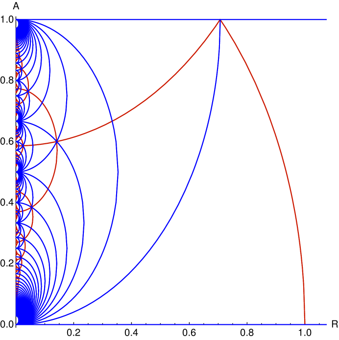
  $$\quad SO(30)\times U(1)^{2}$$

  $$\quad SU(2)\times SO(30)\times U(1)$$

  $$\quad SO(32)\times U(1)$$

$${\fcolorbox{black}{azul}{\rule{0pt}{3pt}\rule{3pt}{0pt}}}+{\fcolorbox{black}{rojo}{\rule{0pt}{3pt}\rule{3pt}{0pt}}} \quad SU(2)\times SO(32)$$

$${\fcolorbox{black}{azul}{\rule{0pt}{3pt}\rule{3pt}{0pt}}}+{\fcolorbox{black}{azul}{\rule{0pt}{3pt}\rule{3pt}{0pt}}}+{\fcolorbox{black}{rojo}{\rule{0pt}{3pt}\rule{3pt}{0pt}}}+{\fcolorbox{black}{rojo}{\rule{0pt}{3pt}\rule{3pt}{0pt}}} \quad SO(34)$$

Figure 9: $SO(32)$ heterotic with Wilson line $A^{I}=\left(A,0_{15}\right)$

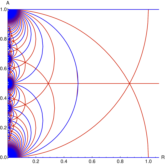
  $$\quad SU(2)\times SO(28)\times U(1)^{2}$$

  $$\quad SU(2)\times SU(2)\times SO(28)\times U(1)$$

  $$\quad SO(32)\times U(1)$$

$${\fcolorbox{black}{azul}{\rule{0pt}{3pt}\rule{3pt}{0pt}}}+{\fcolorbox{black}{rojo}{\rule{0pt}{3pt}\rule{3pt}{0pt}}} \quad SU(2)\times SO(32)$$

$${\fcolorbox{black}{rojo}{\rule{0pt}{3pt}\rule{3pt}{0pt}}}+{\fcolorbox{black}{rojo}{\rule{0pt}{3pt}\rule{3pt}{0pt}}}+{\fcolorbox{black}{rojo}{\rule{0pt}{3pt}\rule{3pt}{0pt}}} \quad SU(2)\times SU(3)\times SO(28)$$

Figure 10: $SO(32)$ heterotic with Wilson line $A^{I}=\left((A)_{2},0_{14}\right)$

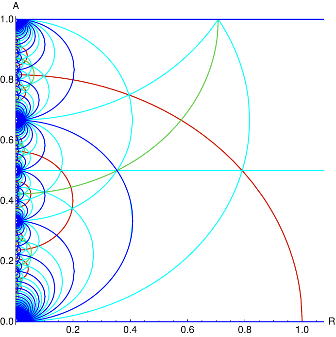
  $$\quad SU(3)\times SO(26)\times U(1)^{2}$$

  $$\quad SU(2)\times SU(3)\times SO(26)\times U(1)$$

  $$\quad SO(6)\times SO(26)\times U(1)$$

  $$\quad SU(3)\times SO(28)\times U(1)$$

  $$\quad SO(32)\times U(1)$$

$${\fcolorbox{black}{cyan}{\rule{0pt}{3pt}\rule{3pt}{0pt}}}+{\fcolorbox{black}{cyan}{\rule{0pt}{3pt}\rule{3pt}{0pt}}}+{\fcolorbox{black}{rojo}{\rule{0pt}{3pt}\rule{3pt}{0pt}}} \quad SU(5)\times SO(26)$$

$${\fcolorbox{black}{cyan}{\rule{0pt}{3pt}\rule{3pt}{0pt}}}+{\fcolorbox{black}{cyan}{\rule{0pt}{3pt}\rule{3pt}{0pt}}}+{\fcolorbox{black}{azul}{\rule{0pt}{3pt}\rule{3pt}{0pt}}}+{\fcolorbox{black}{verde}{\rule{0pt}{3pt}\rule{3pt}{0pt}}} \quad SO(34)$$

$${\fcolorbox{black}{rojo}{\rule{0pt}{3pt}\rule{3pt}{0pt}}}+{\fcolorbox{black}{verde}{\rule{0pt}{3pt}\rule{3pt}{0pt}}} \quad SU(2)\times SU(3)\times SO(28)$$

$${\fcolorbox{black}{rojo}{\rule{0pt}{3pt}\rule{3pt}{0pt}}}+{\fcolorbox{black}{azul}{\rule{0pt}{3pt}\rule{3pt}{0pt}}} \quad SU(2)\times SO(32)$$

Figure 11: $SO(32)$ heterotic with Wilson line $A^{I}=\left((A)_{3},0_{13}\right)$

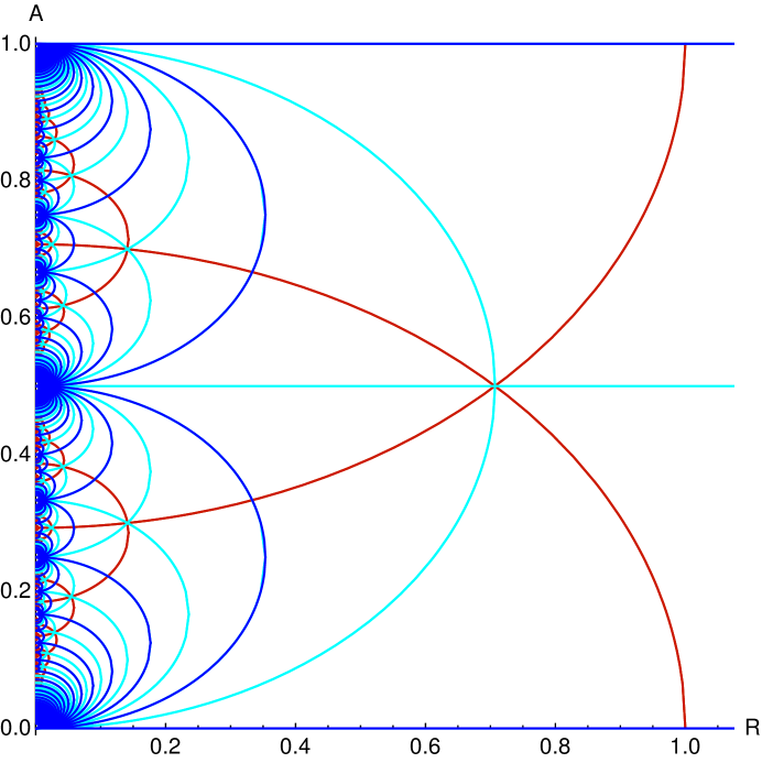
  $$\quad SU(4)\times SO(24)\times U(1)^{2}$$

  $$\quad SU(2)\times SU(4)\times SO(24)\times U(1)$$

  $$\quad SO(8)\times SO(24)\times U(1)$$

  $$\quad SO(32)\times U(1)$$

$${\fcolorbox{black}{cyan}{\rule{0pt}{3pt}\rule{3pt}{0pt}}}+{\fcolorbox{black}{cyan}{\rule{0pt}{3pt}\rule{3pt}{0pt}}}+{\fcolorbox{black}{rojo}{\rule{0pt}{3pt}\rule{3pt}{0pt}}}+{\fcolorbox{black}{rojo}{\rule{0pt}{3pt}\rule{3pt}{0pt}}} \quad SO(10)\times SO(24)$$

$${\fcolorbox{black}{rojo}{\rule{0pt}{3pt}\rule{3pt}{0pt}}}+{\fcolorbox{black}{azul}{\rule{0pt}{3pt}\rule{3pt}{0pt}}} \quad SU(2)\times SO(32)$$

Figure 12: $SO(32)$ heterotic with Wilson line $A^{I}=\left((A)_{4},0_{12}\right)$

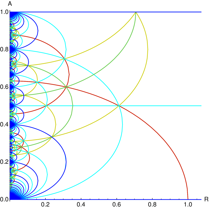
  $$\quad SU(5)\times SO(22)\times U(1)^{2}$$

  $$\quad SU(2)\times SU(5)\times SO(22)\times U(1)$$

  $$\quad SU(6)\times SO(22)\times U(1)$$

  $$\quad SO(10)\times SO(22)\times U(1)$$

  $$\quad SU(5)\times SO(24)\times U(1)$$

  $$\quad SO(32)\times U(1)$$

$${\fcolorbox{black}{cyan}{\rule{0pt}{3pt}\rule{3pt}{0pt}}}+{\fcolorbox{black}{cyan}{\rule{0pt}{3pt}\rule{3pt}{0pt}}}+{\fcolorbox{black}{amarillo}{\rule{0pt}{3pt}\rule{3pt}{0pt}}}+{\fcolorbox{black}{rojo}{\rule{0pt}{3pt}\rule{3pt}{0pt}}} \quad E_{6}\times SO(22)$$

$${\fcolorbox{black}{amarillo}{\rule{0pt}{3pt}\rule{3pt}{0pt}}}+{\fcolorbox{black}{amarillo}{\rule{0pt}{3pt}\rule{3pt}{0pt}}}+{\fcolorbox{black}{azul}{\rule{0pt}{3pt}\rule{3pt}{0pt}}}+{\fcolorbox{black}{verde}{\rule{0pt}{3pt}\rule{3pt}{0pt}}} \quad SO(34)$$

$${\fcolorbox{black}{rojo}{\rule{0pt}{3pt}\rule{3pt}{0pt}}}+{\fcolorbox{black}{rojo}{\rule{0pt}{3pt}\rule{3pt}{0pt}}}+{\fcolorbox{black}{verde}{\rule{0pt}{3pt}\rule{3pt}{0pt}}}+{\fcolorbox{black}{verde}{\rule{0pt}{3pt}\rule{3pt}{0pt}}} \quad SU(5)\times SO(26)$$

$${\fcolorbox{black}{cyan}{\rule{0pt}{3pt}\rule{3pt}{0pt}}}+{\fcolorbox{black}{verde}{\rule{0pt}{3pt}\rule{3pt}{0pt}}} \quad SO(10)\times SO(24)$$

$${\fcolorbox{black}{rojo}{\rule{0pt}{3pt}\rule{3pt}{0pt}}}+{\fcolorbox{black}{azul}{\rule{0pt}{3pt}\rule{3pt}{0pt}}} \quad SU(2)\times SO(32)$$

Figure 13: $SO(32)$ heterotic with Wilson line $A^{I}=\left((A)_{5},0_{11}\right)$

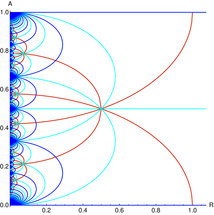
  $$\quad SU(6)\times SO(20)\times U(1)^{2}$$

  $$\quad SU(2)\times SU(6)\times SO(20)\times U(1)$$

  $$\quad SO(12)\times SO(20)\times U(1)$$

  $$\quad SO(32)\times U(1)$$

$${\fcolorbox{black}{rojo}{\rule{0pt}{3pt}\rule{3pt}{0pt}}}+{\fcolorbox{black}{azul}{\rule{0pt}{3pt}\rule{3pt}{0pt}}} \quad SU(2)\times SO(32)$$

$${\fcolorbox{black}{cyan}{\rule{0pt}{3pt}\rule{3pt}{0pt}}}+{\fcolorbox{black}{cyan}{\rule{0pt}{3pt}\rule{3pt}{0pt}}} +{\fcolorbox{black}{cyan}{\rule{0pt}{3pt}\rule{3pt}{0pt}}}+{\fcolorbox{black}{rojo}{\rule{0pt}{3pt}\rule{3pt}{0pt}}}+{\fcolorbox{black}{rojo}{\rule{0pt}{3pt}\rule{3pt}{0pt}}}+{\fcolorbox{black}{rojo}{\rule{0pt}{3pt}\rule{3pt}{0pt}}}\quad E_{7}\times SO(20)$$

Figure 14: $SO(32)$ heterotic with Wilson line $A^{I}=\left((A)_{6},0_{10}\right)$

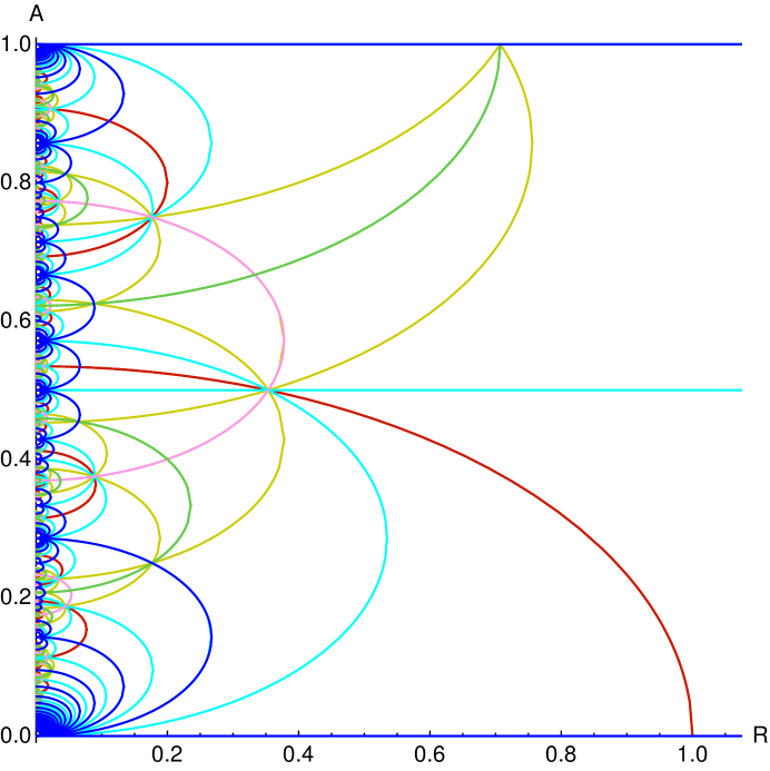
  $$\quad SU(7)\times SO(18)\times U(1)^{2}$$

  $$\quad SU(2)\times SU(7)\times SO(18)\times U(1)$$

  $$\quad SO(32)\times U(1)$$

  $$\quad SU(7)\times SO(20)\times U(1)$$

  $$\quad SO(14)\times SO(18)\times U(1)$$

  $$\quad SU(8)\times SO(18)\times U(1)$$

  $$\quad E_{7}\times SO(18)\times U(1)$$

$${\fcolorbox{black}{amarillo}{\rule{0pt}{3pt}\rule{3pt}{0pt}}}+{\fcolorbox{black}{amarillo}{\rule{0pt}{3pt}\rule{3pt}{0pt}}}+{\fcolorbox{black}{verde}{\rule{0pt}{3pt}\rule{3pt}{0pt}}}+{\fcolorbox{black}{azul}{\rule{0pt}{3pt}\rule{3pt}{0pt}}} \quad SO(34)$$

$${\fcolorbox{black}{azul}{\rule{0pt}{3pt}\rule{3pt}{0pt}}}+{\fcolorbox{black}{rojo}{\rule{0pt}{3pt}\rule{3pt}{0pt}}} \quad SU(2)\times SO(32)$$

$${\fcolorbox{black}{amarillo}{\rule{0pt}{3pt}\rule{3pt}{0pt}}}+{\fcolorbox{black}{amarillo}{\rule{0pt}{3pt}\rule{3pt}{0pt}}}+{\fcolorbox{black}{cyan}{\rule{0pt}{3pt}\rule{3pt}{0pt}}}+{\fcolorbox{black}{cyan}{\rule{0pt}{3pt}\rule{3pt}{0pt}}}+{\fcolorbox{black}{rojo}{\rule{0pt}{3pt}\rule{3pt}{0pt}}}+{\fcolorbox{black}{rosa}{\rule{0pt}{3pt}\rule{3pt}{0pt}}} \quad E_{8}\times SO(18)$$

$${\fcolorbox{black}{rosa}{\rule{0pt}{3pt}\rule{3pt}{0pt}}}+{\fcolorbox{black}{verde}{\rule{0pt}{3pt}\rule{3pt}{0pt}}} \quad E_{7}\times SO(20)$$

Figure 15: $SO(32)$ heterotic with Wilson line $A^{I}=\left((A)_{7},0_{9}\right)$

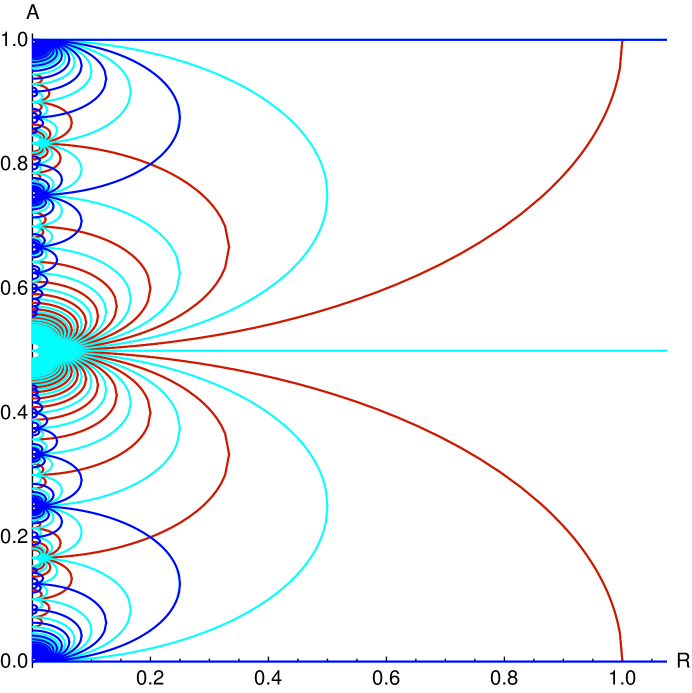
  $$\quad SU(8)\times SO(16)\times U(1)^{2}$$

  $$\quad SU(2)\times SU(8)\times SO(16)\times U(1)$$

  $$\quad SO(16)\times SO(16)\times U(1)$$

  $$\quad SO(32)\times U(1)$$

$${\fcolorbox{black}{rojo}{\rule{0pt}{3pt}\rule{3pt}{0pt}}}+{\fcolorbox{black}{blue}{\rule{0pt}{3pt}\rule{3pt}{0pt}}} \quad SU(2)\times SO(32)$$

Figure 16: $SO(32)$ heterotic with Wilson line $A^{I}=\left((A)_{8},0_{8}\right)$

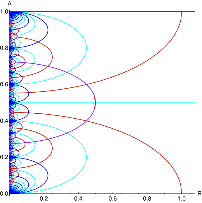
  $$\quad SU(10)\times SO(12)\times U(1)^{2}$$

  $$\quad SU(2)\times SU(10)\times SO(12)\times U(1)$$

  $$\quad SO(20)\times SO(12)\times U(1)$$

  $$\quad SO(32)\times U(1)$$

  $$\quad SU(10)\times E_{7}\times U(1)$$

$${\fcolorbox{black}{violeta}{\rule{0pt}{3pt}\rule{3pt}{0pt}}}+{\fcolorbox{black}{cyan}{\rule{0pt}{3pt}\rule{3pt}{0pt}}} \quad SO(20)\times E_{7}$$

$${\fcolorbox{black}{violeta}{\rule{0pt}{3pt}\rule{3pt}{0pt}}}+{\fcolorbox{black}{rojo}{\rule{0pt}{3pt}\rule{3pt}{0pt}}} \quad SU(2)\times SU(10)\times E_{7}$$

$${\fcolorbox{black}{blue}{\rule{0pt}{3pt}\rule{3pt}{0pt}}}+{\fcolorbox{black}{rojo}{\rule{0pt}{3pt}\rule{3pt}{0pt}}} \quad SU(2)\times SO(32)$$

Figure 18: $SO(32)$ heterotic with Wilson line $A^{I}=\left((A)_{10},0_{6}\right)$

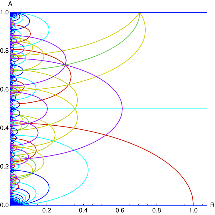
  $$\quad SU(11)\times SO(10)\times U(1)^{2}$$

  $$\quad SU(2)\times SU(11)\times SO(10)\times U(1)$$

  $$\quad SU(12)\times SO(10)\times U(1)$$

  $$\quad SO(22)\times SO(10)\times U(1)$$

  $$\quad SU(11)\times SO(12)\times U(1)$$

  $$\quad SO(32)\times U(1)$$

  $$\quad SU(11)\times E_{6}\times U(1)$$

$${\fcolorbox{black}{rojo}{\rule{0pt}{3pt}\rule{3pt}{0pt}}}+{\fcolorbox{black}{amarillo}{\rule{0pt}{3pt}\rule{3pt}{0pt}}} \quad SU(2)\times SU(12)\times SO(10)\times U(1)$$

$${\fcolorbox{black}{azul}{\rule{0pt}{3pt}\rule{3pt}{0pt}}}+{\fcolorbox{black}{verde}{\rule{0pt}{3pt}\rule{3pt}{0pt}}}+{\fcolorbox{black}{amarillo}{\rule{0pt}{3pt}\rule{3pt}{0pt}}}+{\fcolorbox{black}{amarillo}{\rule{0pt}{3pt}\rule{3pt}{0pt}}} \quad SO(34)$$

$${\fcolorbox{black}{violeta}{\rule{0pt}{3pt}\rule{3pt}{0pt}}}+{\fcolorbox{black}{violeta}{\rule{0pt}{3pt}\rule{3pt}{0pt}}}+{\fcolorbox{black}{verde}{\rule{0pt}{3pt}\rule{3pt}{0pt}}}+{\fcolorbox{black}{rojo}{\rule{0pt}{3pt}\rule{3pt}{0pt}}} \quad SU(11)\times E_{7}$$

$${\fcolorbox{black}{cyan}{\rule{0pt}{3pt}\rule{3pt}{0pt}}}+{\fcolorbox{black}{amarillo}{\rule{0pt}{3pt}\rule{3pt}{0pt}}}+{\fcolorbox{black}{amarillo}{\rule{0pt}{3pt}\rule{3pt}{0pt}}} \quad SO(24)\times SO(10)$$

$${\fcolorbox{black}{rojo}{\rule{0pt}{3pt}\rule{3pt}{0pt}}}+{\fcolorbox{black}{amarillo}{\rule{0pt}{3pt}\rule{3pt}{0pt}}}+{\fcolorbox{black}{amarillo}{\rule{0pt}{3pt}\rule{3pt}{0pt}}} \quad SU(13)\times SO(10)$$

$${\fcolorbox{black}{violeta}{\rule{0pt}{3pt}\rule{3pt}{0pt}}}+{\fcolorbox{black}{cyan}{\rule{0pt}{3pt}\rule{3pt}{0pt}}} \quad SO(22)\times E_{6}$$

$${\fcolorbox{black}{violeta}{\rule{0pt}{3pt}\rule{3pt}{0pt}}}+{\fcolorbox{black}{amarillo}{\rule{0pt}{3pt}\rule{3pt}{0pt}}} \quad SU(12)\times E_{6}$$

$${\fcolorbox{black}{violeta}{\rule{0pt}{3pt}\rule{3pt}{0pt}}}+{\fcolorbox{black}{rojo}{\rule{0pt}{3pt}\rule{3pt}{0pt}}} \quad SU(2)\times SU(11)\times E_{6}$$

$${\fcolorbox{black}{azul}{\rule{0pt}{3pt}\rule{3pt}{0pt}}}+{\fcolorbox{black}{rojo}{\rule{0pt}{3pt}\rule{3pt}{0pt}}} \quad SU(2)\times SO(32)$$

Figure 19: $SO(32)$ heterotic with Wilson line $A^{I}=\left((A)_{11},0_{5}\right)$

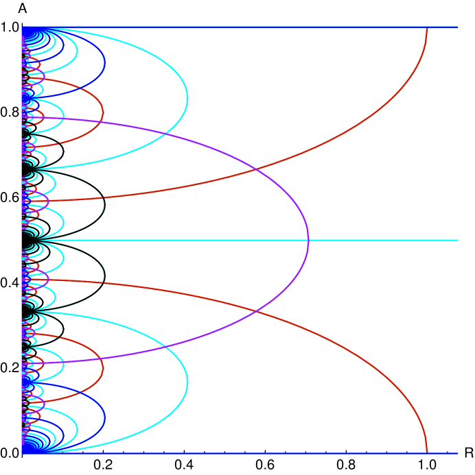
  $$\quad SU(12)\times SO(8)\times U(1)^{2}$$

  $$\quad SU(2)\times SU(12)\times SO(8)\times U(1)$$

  $$\quad SO(24)\times SO(8)\times U(1)$$

   $$\quad SO(32)\times U(1)$$

  $$\quad SU(12)\times SO(10)\times U(1)$$

$${\fcolorbox{black}{azul}{\rule{0pt}{3pt}\rule{-2pt}{0pt}}\fcolorbox{black}{negro}{\rule{0pt}{3pt}\rule{-2pt}{0pt}}}+{\fcolorbox{black}{rojo}{\rule{0pt}{3pt}\rule{3pt}{0pt}}} \quad SU(2)\times SO(32)$$

$${\fcolorbox{black}{violeta}{\rule{0pt}{3pt}\rule{3pt}{0pt}}}+{\fcolorbox{black}{rojo}{\rule{0pt}{3pt}\rule{3pt}{0pt}}} \quad SU(2)\times SU(12)\times SO(10)$$

$${\fcolorbox{black}{violeta}{\rule{0pt}{3pt}\rule{3pt}{0pt}}}+{\fcolorbox{black}{cyan}{\rule{0pt}{3pt}\rule{3pt}{0pt}}} \quad SO(24)\times SO(10)$$

Figure 20: $SO(32)$ heterotic with Wilson line $A^{I}=\left((A)_{12},0_{4}\right)$

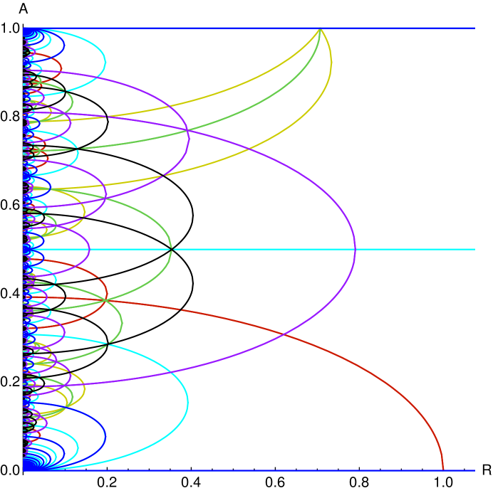
  $$\quad SU(13)\times SO(6)\times U(1)^{2}$$

  $$\quad SU(2)\times SU(13)\times SO(6)\times U(1)$$

  $$\quad SU(14)\times SO(6)\times U(1)$$

  $$\quad SO(26)\times SO(6)\times U(1)$$

  $$\quad SU(13)\times SO(8)\times U(1)$$

  $$\quad SO(32)\times U(1)$$

  $$\quad SU(13)\times SU(5)\times U(1)$$

  $$\quad SU(17)\times U(1)$$

$${\fcolorbox{black}{azul}{\rule{0pt}{3pt}\rule{3pt}{0pt}}}+{\fcolorbox{black}{verde}{\rule{0pt}{3pt}\rule{3pt}{0pt}}}+{\fcolorbox{black}{amarillo}{\rule{0pt}{3pt}\rule{3pt}{0pt}}}+{\fcolorbox{black}{amarillo}{\rule{0pt}{3pt}\rule{3pt}{0pt}}} \quad SO(34)$$

$${\fcolorbox{black}{violeta}{\rule{0pt}{3pt}\rule{3pt}{0pt}}}+{\fcolorbox{black}{violeta}{\rule{0pt}{3pt}\rule{3pt}{0pt}}}+{\fcolorbox{black}{verde}{\rule{0pt}{3pt}\rule{3pt}{0pt}}} \quad SU(13)\times SO(10)$$

$${\fcolorbox{black}{negro}{\rule{0pt}{3pt}\rule{3pt}{0pt}}}+{\fcolorbox{black}{negro}{\rule{0pt}{3pt}\rule{3pt}{0pt}}}+{\fcolorbox{black}{verde}{\rule{0pt}{3pt}\rule{3pt}{0pt}}}+{\fcolorbox{black}{cyan}{\rule{0pt}{3pt}\rule{3pt}{0pt}}} \quad SO(28)\times SO(6)$$

$${\fcolorbox{black}{rojo}{\rule{0pt}{3pt}\rule{3pt}{0pt}}}+{\fcolorbox{black}{violeta}{\rule{0pt}{3pt}\rule{3pt}{0pt}}} \quad SU(2)\times SU(13)\times SU(5)$$

$${\fcolorbox{black}{rojo}{\rule{0pt}{3pt}\rule{3pt}{0pt}}}+{\fcolorbox{black}{rojo}{\rule{0pt}{3pt}\rule{3pt}{0pt}}}+{\fcolorbox{black}{verde}{\rule{0pt}{3pt}\rule{3pt}{0pt}}}+{\fcolorbox{black}{verde}{\rule{0pt}{3pt}\rule{3pt}{0pt}}} \quad SU(13)\times SO(10)$$

$${\fcolorbox{black}{rojo}{\rule{0pt}{3pt}\rule{3pt}{0pt}}}+{\fcolorbox{black}{azul}{\rule{0pt}{3pt}\rule{3pt}{0pt}}} \quad SU(2)\times SO(32)$$

$${\fcolorbox{black}{negro}{\rule{0pt}{3pt}\rule{3pt}{0pt}}}+{\fcolorbox{black}{rojo}{\rule{0pt}{3pt}\rule{3pt}{0pt}}} \quad SU(2)\times SU(2)\times SU(17)$$

$${\fcolorbox{black}{violeta}{\rule{0pt}{3pt}\rule{3pt}{0pt}}}+{\fcolorbox{black}{cyan}{\rule{0pt}{3pt}\rule{3pt}{0pt}}} \quad SO(26)\times SU(5)$$

$${\fcolorbox{black}{negro}{\rule{0pt}{3pt}\rule{3pt}{0pt}}}+{\fcolorbox{black}{amarillo}{\rule{0pt}{3pt}\rule{3pt}{0pt}}}+{\fcolorbox{black}{violeta}{\rule{0pt}{3pt}\rule{3pt}{0pt}}} \quad SU(18)$$

$${\fcolorbox{black}{violeta}{\rule{0pt}{3pt}\rule{3pt}{0pt}}}+{\fcolorbox{black}{amarillo}{\rule{0pt}{3pt}\rule{3pt}{0pt}}} \quad SU(14)\times SU(5)$$

Figure 21: $SO(32)$ heterotic with Wilson line $A^{I}=\left((A)_{13},0_{3}\right)$

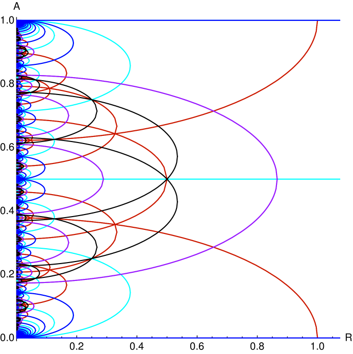
  $$\quad SU(14)\times SO(4)\times U(1)^{2}$$

  $$\quad SU(2)\times SU(14)\times SO(4)\times U(1)$$

  $$\quad SO(28)\times SO(4)\times U(1)$$

  $$\quad SO(32)\times U(1)$$

  $$\quad SU(14)\times SU(3)\times SU(2)\times U(1)$$

  $$\quad SU(16)\times SU(2)\times U(1)$$

$${\fcolorbox{black}{negro}{\rule{0pt}{3pt}\rule{3pt}{0pt}}}+{\fcolorbox{black}{negro}{\rule{0pt}{3pt}\rule{3pt}{0pt}}}+{\fcolorbox{black}{cyan}{\rule{0pt}{3pt}\rule{3pt}{0pt}}}+{\fcolorbox{black}{rojo}{\rule{0pt}{3pt}\rule{3pt}{0pt}}} \quad SU(2)\times SO(32)$$

$${\fcolorbox{black}{rojo}{\rule{0pt}{3pt}\rule{3pt}{0pt}}}+{\fcolorbox{black}{rojo}{\rule{0pt}{3pt}\rule{3pt}{0pt}}}+{\fcolorbox{black}{rojo}{\rule{0pt}{3pt}\rule{3pt}{0pt}}} \quad SU(3)\times SU(14)\times SO(4)$$

$${\fcolorbox{black}{violeta}{\rule{0pt}{3pt}\rule{3pt}{0pt}}}+{\fcolorbox{black}{cyan}{\rule{0pt}{3pt}\rule{3pt}{0pt}}} \quad SO(28)\times SU(3)\times SU(2)$$

$${\fcolorbox{black}{rojo}{\rule{0pt}{3pt}\rule{3pt}{0pt}}}+{\fcolorbox{black}{violeta}{\rule{0pt}{3pt}\rule{3pt}{0pt}}} \quad SU(2)\times SU(14)\times SU(3)\times SO(4)$$

$${\fcolorbox{black}{rojo}{\rule{0pt}{3pt}\rule{3pt}{0pt}}}+{\fcolorbox{black}{azul}{\rule{0pt}{3pt}\rule{3pt}{0pt}}} \quad SU(2)\times SO(32)$$

$${\fcolorbox{black}{rojo}{\rule{0pt}{3pt}\rule{3pt}{0pt}}}+{\fcolorbox{black}{negro}{\rule{0pt}{3pt}\rule{3pt}{0pt}}} \quad SU(2)\times SU(16)\times SO(4)$$

Figure 22: $SO(32)$ heterotic with Wilson line $A^{I}=\left((A)_{14},0_{2}\right)$

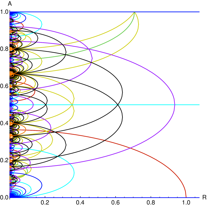
  $$\quad SU(15)\times U(1)^{3}$$

   $$\quad SU(2)\times SU(15)\times U(1)^{2}$$

   $$\quad SU(16)\times U(1)^{2}$$

  $$\quad SO(30)\times U(1)^{2}$$

  $$\quad SU(15)\times SO(4)\times U(1)$$

   $$\quad SO(32)\times U(1)$$

$${\fcolorbox{black}{amarillo}{\rule{0pt}{3pt}\rule{3pt}{0pt}}}+{\fcolorbox{black}{amarillo}{\rule{0pt}{3pt}\rule{3pt}{0pt}}}+{\fcolorbox{black}{verde}{\rule{0pt}{3pt}\rule{3pt}{0pt}}}+{\fcolorbox{black}{azul}{\rule{0pt}{3pt}\rule{3pt}{0pt}}} \quad SO(34)$$

$${\fcolorbox{black}{amarillo}{\rule{0pt}{3pt}\rule{-2pt}{0pt}}\fcolorbox{black}{negro}{\rule{0pt}{3pt}\rule{-2pt}{0pt}}}+{\fcolorbox{black}{amarillo}{\rule{0pt}{3pt}\rule{-2pt}{0pt}}\fcolorbox{black}{negro}{\rule{0pt}{3pt}\rule{-2pt}{0pt}}}+{\fcolorbox{black}{cyan}{\rule{0pt}{3pt}\rule{3pt}{0pt}}} \quad SO(32)\times U(1)$$

$${\fcolorbox{black}{violeta}{\rule{0pt}{3pt}\rule{3pt}{0pt}}}+{\fcolorbox{black}{cyan}{\rule{0pt}{3pt}\rule{3pt}{0pt}}} \quad SU(2)\times SO(30)\times U(1)$$

$${\fcolorbox{black}{amarillo}{\rule{0pt}{3pt}\rule{-2pt}{0pt}}\fcolorbox{black}{negro}{\rule{0pt}{3pt}\rule{-2pt}{0pt}}}+{\fcolorbox{black}{rojo}{\rule{0pt}{3pt}\rule{-2pt}{0pt}}\fcolorbox{black}{violeta}{\rule{0pt}{3pt}\rule{-2pt}{0pt}}} \quad SU(2)\times SU(16)\times U(1)$$

$${\fcolorbox{black}{rojo}{\rule{0pt}{3pt}\rule{3pt}{0pt}}}+{\fcolorbox{black}{azul}{\rule{0pt}{3pt}\rule{-2pt}{0pt}}\fcolorbox{black}{naranja}{\rule{0pt}{3pt}\rule{-2pt}{0pt}}} \quad SU(2)\times SO(32)$$

$${\fcolorbox{black}{rojo}{\rule{0pt}{3pt}\rule{3pt}{0pt}}}+{\fcolorbox{black}{violeta}{\rule{0pt}{3pt}\rule{3pt}{0pt}}} \quad SO(4)\times SU(15)\times U(1)$$

$${\fcolorbox{black}{rojo}{\rule{0pt}{3pt}\rule{3pt}{0pt}}}+{\fcolorbox{black}{negro}{\rule{0pt}{3pt}\rule{3pt}{0pt}}}+{\fcolorbox{black}{negro}{\rule{0pt}{3pt}\rule{3pt}{0pt}}} \quad SU(17)\times U(1)$$

$${\fcolorbox{black}{verde}{\rule{0pt}{3pt}\rule{3pt}{0pt}}}+{\fcolorbox{black}{negro}{\rule{0pt}{3pt}\rule{3pt}{0pt}}}+{\fcolorbox{black}{negro}{\rule{0pt}{3pt}\rule{3pt}{0pt}}} \quad SU(2)\times SU(17)$$

$${\fcolorbox{black}{violeta}{\rule{0pt}{3pt}\rule{3pt}{0pt}}}+{\fcolorbox{black}{negro}{\rule{0pt}{3pt}\rule{3pt}{0pt}}}+{\fcolorbox{black}{amarillo}{\rule{0pt}{3pt}\rule{3pt}{0pt}}} \quad SO(4)\times SU(16)$$

$${\fcolorbox{black}{violeta}{\rule{0pt}{3pt}\rule{3pt}{0pt}}}+{\fcolorbox{black}{violeta}{\rule{0pt}{3pt}\rule{3pt}{0pt}}}+{\fcolorbox{black}{verde}{\rule{0pt}{3pt}\rule{3pt}{0pt}}} \quad SU(15)\times SU(3)\times SU(2)$$

Figure 23: $SO(32)$ heterotic with Wilson line $A^{I}=\left((A)_{15},0\right)$

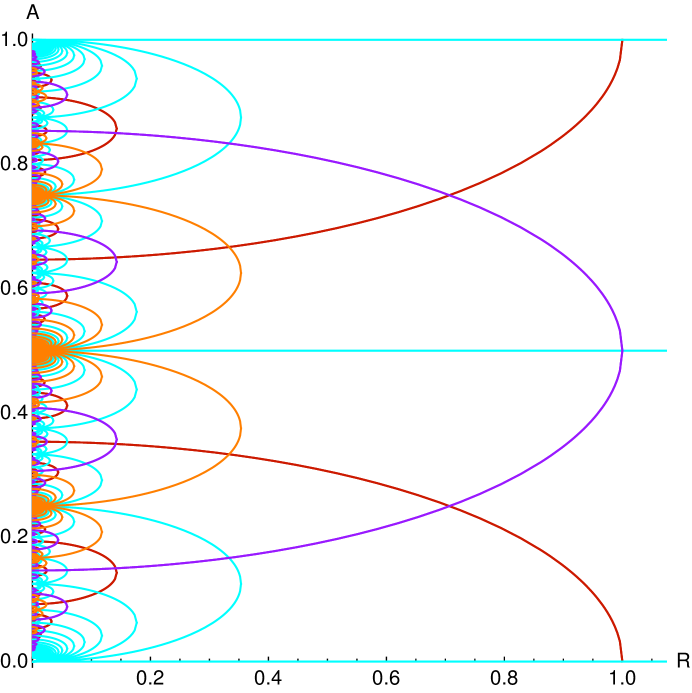
  $$\quad SU(16)\times U(1)^{2}$$

   $$\quad SU(2)\times SU(16)\times U(1)$$

   $$\quad SO(32)\times U(1)$$

$${\fcolorbox{black}{rojo}{\rule{0pt}{3pt}\rule{-2pt}{0pt}}\fcolorbox{black}{violeta}{\rule{0pt}{3pt}\rule{-2pt}{0pt}}}+{\fcolorbox{black}{cyan}{\rule{0pt}{3pt}\rule{-2pt}{0pt}}\fcolorbox{black}{naranja}{\rule{0pt}{3pt}\rule{-2pt}{0pt}}} \quad SU(2)\times SO(32)$$

$${\fcolorbox{black}{violeta}{\rule{0pt}{3pt}\rule{3pt}{0pt}}}+{\fcolorbox{black}{rojo}{\rule{0pt}{3pt}\rule{3pt}{0pt}}} \quad SO(4)\times SU(16)$$

Figure 24: $SO(32)$ heterotic with Wilson line $A^{I}=\left((A)_{16}\right)$

For Wilson lines of type $A^{I}=\left(\left(A\right)_{p},0_{16-p}\right)$ there are families of curves of enhancement parameterized by three integer numbers $\alpha$, $\beta$ and $\delta$. Inside each family there are different curves corresponding to different winding numbers and different integer values for $q$. If $R$ is sufficiently small then $w$ can be arbitrarily large.

$$A_{w,\alpha,\beta,\delta}(R) = \frac{pq+\alpha-\tfrac{p\delta}{2}\pm\sqrt{\left(\alpha-\tfrac{p\delta}{2}\right)^{2}-p\left(|\alpha|-\delta\alpha+\beta+4\delta-2+2w^{2}R^{2}\right)}}{pw}$$ (D.1)

$$= \frac{pq+\mu\pm\sqrt{\mu^{2}-p\left(\lambda+2w^{2}R^{2}\right)}}{pw}\,,$$

where we defined:

$$\mu\ =\ \alpha-\frac{p\delta}{2}\qquad{\rm and}\qquad\lambda\ =\ |\alpha|-\delta\alpha+\beta+4\delta-2\,.$$

The massless states associated with each family of curves are

$$\pi=\left(\underline{(q\pm(1-\tfrac{3}{2}\delta))_{\alpha},(q\pm\tfrac{1}{2}\delta)_{p-{\alpha}}},\underline{\beta\pm\tfrac{1}{2}\delta,(\pm\tfrac{1}{2}\delta)_{15-p}}\right)\,.$$ (D.2)

The possible values of the parameters are listed in the following table, with the colour we use to identify them on the figures and the corresponding gauge group.

Colour	$\delta$	$\beta$	$|\alpha|$	Gauge group
				$A_{p-1}\times D_{16-p}$
	$0$	$0$	$0$	$A_{1}\times A_{p-1}\times D_{16-p}$
	$0$	$0$	$1$	$A_{p}\times D_{16-p}$
	$0$	$0$	$2$	$D_{p}\times D_{16-p}$
	$0$	$0$	$3$	$E_{p}\times D_{16-p}$
	$0$	$1$	$0$	$A_{p-1}\times D_{17-p}$
	$0$	$1$	$1$	$D_{16}$
	$1$	$0$	$0$	$A_{p-1}\times E_{17-p}$
	$1$	$0$	$1$	$D_{16}$ for $p=12$, $A_{16}$ for $p=13$, $A_{15}\times A_{1}$ for $p=14$, $A_{15}\times D_{1}$ for $p=15$
	$1$	$0$	$2$	$D_{16}$

The number of states for each of these curves is given by

$$2\binom{p}{|\alpha|}(32-2p)^{\beta}2^{(15-p+\delta_{p,16})\delta}\,.$$ (D.3)

The allowed values for $q$ and $w$ are the ones that satisfy the quantization condition

$$\frac{pq^{2}+2\mu q+\lambda}{2w}\in\mathbb{Z}\,.$$ (D.4)

For arbitrary $A$, we get the $3p^{2}-63p+480$ roots of $U(1)^{2}\times SU(p)\times SO(32-2p)$. If $A$ is half-integer we get the $4p^{2}-64p+480$ roots of $U(1)\times SO(2p)\times SO(32-2p)$, so we can think of them as part of the family with $(\delta,\beta,\alpha)=(0,0,2)$ and $w=0$ which give $p^{2}-p$ additional states. For $p=2$ $(0,0,2)$ is equivalent to $(0,0,0)$.

If $A_{1}$ is integer we get the $480$ roots of $SO(32)\times U(1)$, so we can think of them as part of the family with $(\delta,\beta,\alpha)=(0,1,1)$ and $w=0$ superimposed with another one of the family with $(\delta,\beta,\alpha)=(0,0,2)$ and $w=0$, which give $63p-3p^{2}=(64p-4p^{2})+(p^{2}-p)$ additional states. For $p=16$ we only have the $(0,0,2)$. We can classify some of the enhancements by the colours of the curves that intersect, we list them on the table below:

Colours	Gauge group
${\fcolorbox{black}{rojo}{\rule{0pt}{3pt}\rule{3pt}{0pt}}}+{\fcolorbox{black}{azul}{\rule{0pt}{3pt}\rule{-2pt}{0pt}}\fcolorbox{black}{naranja}{\rule{0pt}{3pt}\rule{-2pt}{0pt}}}$	$A_{1}\times D_{16}$
${\fcolorbox{black}{rojo}{\rule{0pt}{3pt}\rule{3pt}{0pt}}}+{\fcolorbox{black}{violeta}{\rule{0pt}{3pt}\rule{3pt}{0pt}}}$	$A_{1}\times A_{p-1}\times E_{17-p}$
${\fcolorbox{black}{cyan}{\rule{0pt}{3pt}\rule{3pt}{0pt}}}+{\fcolorbox{black}{violeta}{\rule{0pt}{3pt}\rule{3pt}{0pt}}}$	$E_{p+1}\times D_{16-p}$
${\fcolorbox{black}{violeta}{\rule{0pt}{3pt}\rule{3pt}{0pt}}}+{\fcolorbox{black}{amarillo}{\rule{0pt}{3pt}\rule{3pt}{0pt}}}$	$A_{p}\times E_{17-p}$
${\fcolorbox{black}{rojo}{\rule{0pt}{3pt}\rule{3pt}{0pt}}}+{\fcolorbox{black}{rojo}{\rule{0pt}{3pt}\rule{3pt}{0pt}}}+{\fcolorbox{black}{rojo}{\rule{0pt}{3pt}\rule{3pt}{0pt}}}$	$A_{2}\times A_{p-1}\times D_{16-p}$

D.2 Relation to generalized Dynkin diagrams

Here we show how some of the previous enhancement curves and points can be obtained from the generalized Dynkin diagram in (B.3).

For Wilson lines of the form $(0_{16-p},(A)_{p})$ and at any radius, then the inequality $-A_{2}\leq A_{1}$, as well as all the $A_{i}\leq A_{i+1}$ inequalities are saturated except for $A_{16-p}=A_{17-p}$. This means that the gauge group is given by the generalized diagram with all the nodes except for $16$, $18$, $19$ and $16-p$. Then the diagram that gives the enhancement symmetry is:

(D.5)

which corresponds to the $A_{p-1}\times D_{16-p}(\times U(1)^{2})=SU(p)\times SO(32-2p)(\times U(1)^{2})$ at a generic value of $A$ and $R$. Choosing particular values for them, we can saturate one or more inequalities associated to the missing nodes. To obtain the horizontal lines we have to pick an arbitrary $R$, which discards the nodes $18$ and $19$. To get the nodes $16-p$ or $16$ we have only one possibility: $A=0$ for the former, and $A=\tfrac{1}{2}$ for the latter. We get, respectively:

(D.6)

(D.7)

and hence the gauge groups are $D_{16}=SO(32)$ ($\times U(1)$) and $D_{p}\times D_{16-p}=SO(2p)\times SO(32-2p)$ ($\times U(1)$) (blue and cyan lines). Finally, choosing a specific value of $R$, the inequality associated to the $18$th or $19$th node (not both at the same time) can be saturated. This gives maximal enhancements. In the $D_{16}$ case, the only possibility is to add the $18$th node, which gives $A_{1}\times D_{16}$ (intersection between a blue and a red curve):

(D.8)

In the $D_{p}\times D_{16-p}$ case, one can add the $18$th or the $19$th node, depending on which part of the diagram has less than $8$ nodes

(D.9)

(D.10)

This accounts for $D_{p}\times E_{17-p}$ (intersection between a cyan and other curves) and $E_{p+1}\times D_{16-p}$ (intersection between a cyan and a purple curve).

For $R(A)$ (with arbitrary $A$) saturating the inequality associated to the $18$th node, we obtain $A_{1}\times A_{p-1}\times D_{16-p}$ (red curves):

(D.11)

And in particular for $A=\tfrac{4}{p}$, we have:

(D.12)

which gives the gauge group $A_{1}\times E_{17-p}\times A_{p-1}$, considered in section 3.2.4 and seen in the figures at the intersections between the red and purple curves.

On the other hand, choosing $R(A)$ so that it saturates the inequality associated to the $19$th node, we obtain $E_{17-p}\times A_{p-1}$ (purple curves):

(D.13)

Then we can colour the dots on the generalized Dynkin diagram depending on which curves saturate their inequality:

(D.14)

The enhancements corresponding to each curve are obtained by removing all the coloured nodes except the node with that colour. The intersection of curves give the group associated to the diagram obtained by keeping the nodes with the colours of the involved curves.

Something odd happens for $p=1$

(D.15)

For generic $A$ and $R$, this is $D_{15}$. For $A=1$ (cyan dot) we get $D_{16}$ and if we also take $R^{2}=\tfrac{1}{2}$ (red dot) we get $D_{17}$. If, on the other hand, we take $A=0$ (blue dot) then we get $D_{16}$ and if we also select $R^{2}=1$ (red dot) we get $A_{1}\times D_{16}$. If we only take the appropriate $R$ to have the red dot, then we get $A_{1}\times D_{15}$. To compare with figure 9 we have to take into account that the cyan solutions are not well defined for $p<2$, and then we see them as blue curves.

For $p=15$, the equation for the seventh node no longer holds, and then we have:

(D.16)

For generic $A$ and $R$ this is $A_{14}$. Selecting a specific $R$, we can turn on the red and/or the purple nodes to get $A_{1}\times A_{14}$ or $D_{2}\times A_{14}$. Selecting $A=\tfrac{1}{2}$ (cyan dot) we obtain $D_{15}$ and for $A=0$ both blue dots are turned on and we get $D_{16}$. Only choosing $R=1$ (red dot) we get $A_{1}\times D_{16}$.

For $p=16$ we have a very different situation:

(D.17)

For generic $A$ and $R$ this is $A_{15}$. Selecting a specific $R$, the red and/or the purple nodes are turned on and we get $A_{1}\times A_{15}$ or $D_{2}\times A_{15}$. Selecting $A=\tfrac{1}{2}$ (cyan dot) we obtain $D_{16}$ and for $A=0$ (orange dot) we get $D_{16}$. Only choosing $R=1$ (red or purple dot) we get $A_{1}\times D_{16}$.

The enhancements of the curves that correspond to the other colours cannot be obtained with this construction. On one hand we see from the figures that the Wilson lines that give these curves are not in the fundamental region in the conventions of Appendix B. On the other hand, if this region is the fundamental region, it should contain all the possible enhancement groups, and as such all the curves with the different colours. However, it is easy to see that using this method, the Wilson lines in the fundamental region that give the missing enhancement groups are not of the form chosen, with $p$ equal components and the other zero. For example, to obtain the enhancement $A_{p}\times D_{16-p}$ corresponding to the yellow curves, we would need to replace the $15$th node with the $16$th one (and then add the 18th one), which requires $A_{16}=1-A_{15}$ which is not within the ansatz chosen for the Wilson lines.

D.3 Slices for the $E_{8}\times E_{8}$ theory

We applied the method based on generalized Dynkin diagrams used to obtain the slices of moduli space containing desired enhanement groups, to the case of $\Gamma_{8}\times\Gamma_{8}$. This forces us to consider now also Wilson lines where some of the components are of the form $1-A$. The slices shown in the figures contain most of the enhacement groups discussed in the main text.

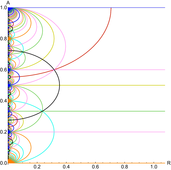
  $$\quad SO(16)\times SU(5)\times SO(6)\times U(1)^{2}$$

  $$\quad SO(18)\times SU(5)\times SO(6)\times U(1)$$

  $$\quad SO(16)\times SO(10)\times SO(6)\times U(1)$$

  $$\quad SO(26)\times SO(6)\times U(1)$$

  $$\quad SO(16)\times SO(16)\times U(1)$$

  $$\quad SO(16)\times SU(5)\times SU(5)$$

  $$\quad SO(16)\times SU(9)$$

  $$\quad SO(16)\times E_{8}$$

  $$\quad SO(24)\times SU(5)$$

$${\fcolorbox{black}{rojo}{\rule{0pt}{3pt}\rule{3pt}{0pt}}}+{\fcolorbox{black}{azul}{\rule{0pt}{3pt}\rule{3pt}{0pt}}} \quad SO(18)\times E_{8}$$

$${\fcolorbox{black}{amarillo}{\rule{0pt}{3pt}\rule{3pt}{0pt}}}+{\fcolorbox{black}{negro}{\rule{0pt}{3pt}\rule{3pt}{0pt}}} \quad SO(24)\times SO(10)$$

$${\fcolorbox{black}{cyan}{\rule{0pt}{3pt}\rule{3pt}{0pt}}}+{\fcolorbox{black}{rosa}{\rule{0pt}{3pt}\rule{3pt}{0pt}}} \quad SO(26)\times SU(5)$$

$${\fcolorbox{black}{rojo}{\rule{0pt}{3pt}\rule{3pt}{0pt}}}+{\fcolorbox{black}{rosa}{\rule{0pt}{3pt}\rule{3pt}{0pt}}}+{\fcolorbox{black}{rosa}{\rule{0pt}{3pt}\rule{3pt}{0pt}}}+{\fcolorbox{black}{negro}{\rule{0pt}{3pt}\rule{3pt}{0pt}}} \quad SO(26)\times SU(5)$$

$${\fcolorbox{black}{cyan}{\rule{0pt}{3pt}\rule{3pt}{0pt}}}+{\fcolorbox{black}{verde}{\rule{0pt}{3pt}\rule{3pt}{0pt}}}+{\fcolorbox{black}{verde}{\rule{0pt}{3pt}\rule{3pt}{0pt}}}+{\fcolorbox{black}{negro}{\rule{0pt}{3pt}\rule{3pt}{0pt}}} \quad SO(34)$$

Figure 28: $\Gamma_{8}\times\Gamma_{8}$ heterotic with Wilson line $A^{I}=\left(A-1,(A)_{4},0_{10},1\right)$

Appendix E More on fixed points and dualities

Here we collect the details of the calculations involved in section 3.5. The transformations $O_{U}$ in (3.44) acting on a vector $Z$ of momentum, winding and “heterotic” momenta, result in the transformed momenta

$$w^{\prime}= r\left(n-\tfrac{1}{2}|A|^{2}w-A\cdot\pi\right)\,,$$ (E.1)

$$n^{\prime}= \left(\tfrac{1}{r}+A^{\prime}UA\right)w+A^{\prime}U\pi-r\tfrac{|A^{\prime}|^{2}}{2}\left(n-\tfrac{1}{2}|A|^{2}w-A\cdot\pi\right)\,,$$

$$\pi^{\prime}= U\pi+UAw-rA^{\prime}\left(n-\tfrac{1}{2}|A|^{2}w-A\cdot\pi\right)\,.$$

Requiring these to be quantized leads to the conditions

$$r,\,\frac{r|A|^{2}}{2},\,\frac{r|A^{\prime}|^{2}}{2}\in\mathbb{Z};$$ (E.2)

$$\frac{1}{r}+A^{\prime}UA+r\frac{|A|^{2}}{2}\frac{|A^{\prime}|^{2}}{2}\in\mathbb{Z} \forall\,\,\pi\in\Gamma,\,\,\pi^{\prime}\in\Gamma^{\prime}:\ \pi^{\prime}U\pi+r(\pi\cdot A)(\pi^{\prime}\cdot A^{\prime})\in\mathbb{Z}\,;$$

$$rA,\,rA^{\prime}\in\Gamma\cap\Gamma^{\prime}\,;\qquad A^{\prime}U+\frac{r|A^{\prime}|^{2}}{2}A\in\Gamma\,;\qquad UA+\frac{r|A|^{2}}{2}A^{\prime}\in\Gamma^{\prime}\,$$

and $U\in O(16,\mathbb{Z})$.

We analyze these in more detail, depending whether the duality acts on the same theory or links two theories with different lattices $\Gamma$ and $\Gamma^{\prime}$.

E.1 $\Gamma\leftrightarrow\Gamma$

For Wilson lines of the form (3.31), and $U$ given by (3.47), the quantization conditions (E.2) become

$$\tfrac{(Q\pm 1)^{2}}{r}\,,\,(Q\pm 1)\sqrt{\tfrac{Q}{2r}}\,,\,\sqrt{\tfrac{Qr}{2}}\in\mathbb{Z}\,,\quad\text{and}\,\,\left\{\begin{matrix}Q\in 2\mathbb{Z}&\text{for}&U=\pm I\\ Q+1\in 2\mathbb{Z}&\text{for}&\,U=U_{\pm}\end{matrix}\right.$$ (E.3)

where $U_{\pm}$ are defined in (3.47),

$$Q\equiv\frac{rA_{1}^{2}}{2}=\left.\frac{1}{2}\frac{A_{1}^{2}}{R^{2}}\right|_{\rm{fp}}=\left.\frac{1}{2}\mathbb{A}^{2}\right|_{\rm fp}$$ (E.4)

and $\mathbb{A}$ is defined in (3.39). Here we have used that for the fixed points $R=R_{\rm{fp}}$, one has $r=R_{\rm{fp}}^{-2}$ since $R^{\prime}=\tfrac{1}{rR}=R$.

For $U=\pm I$ we define $p=\tfrac{(Q\pm 1)^{2}}{r}$and $q=Q/2$, then:

$$p,\ \ q,\ \ r,\ \ \sqrt{pq},\ \ \sqrt{qr}\ \in\ \mathbb{Z};\quad\sqrt{pr}=2q\pm 1\,.$$ (E.5)

Quotienting these equations, we see that $p,q$ $r$ can be written as

$$\sqrt{p}=t\sqrt{k},\quad\sqrt{q}=n\sqrt{k},\quad\sqrt{r}=m\sqrt{k}\,,$$ (E.6)

with $t,n,m,k\in\mathbb{Z}$. Then

$$k^{-1}=\pm(tm-2n^{2})\in\mathbb{Z}\,,$$ (E.7)

which implies $k=1$ and $t=\tfrac{2n^{2}\pm 1}{m}$. Taking into account that $n=\sqrt{\tfrac{Q}{2}}=\tfrac{R^{-1}A_{1}}{2}$ and $m=\sqrt{r}=R^{-1}$ must be integers, the only condition is

$$\frac{2n^{2}\pm 1}{m}\in\mathbb{Z}\,.$$ (E.8)

For $U=U_{\pm}$, defining $p=\tfrac{(Q\pm 1)^{2}}{2r}$ and $s=\tfrac{r}{2}$,

$$p,\ \ Q,\ \ s,\quad\sqrt{pQ},\quad\sqrt{Qs}\in\mathbb{Z}\quad{\rm and}\quad\sqrt{ps}=\tfrac{Q\pm 1}{2}\,,$$ (E.9)

where we have used the fact that as $Q$, $2p$ and $\sqrt{pQ}$ are integers with $Q$ odd, implies that $p$ is also integer. $\tfrac{Q+1}{2}$ is integer, then we have the same situation as in the first case. Analogously

$$\sqrt{p}=t\sqrt{k},\quad\sqrt{Q}=n\sqrt{k},\quad\sqrt{s}=m\sqrt{k}$$ (E.10)

with $t,n,m,k\in\mathbb{Z}$. Then

$$tmk=\tfrac{n^{2}k\pm 1}{2}\,\quad\implies\ \ k^{-1}=\pm(2tm-n^{2})\in\mathbb{Z}\,,$$ (E.11)

but this implies that $k=1$ and $t=\tfrac{n^{2}\pm 1}{2m}$. Then, taking into account that $n=\sqrt{Q}=\tfrac{R^{-1}A_{1}}{\sqrt{2}}$ and $m=\sqrt{\tfrac{r}{2}}=\tfrac{R^{-1}}{\sqrt{2}}$, the only condition is:

$$\frac{n^{2}\pm 1}{2m}\in\mathbb{Z}$$ (E.12)

The possible values of $m$ and $n$ that verify these conditions with the plus signs give the fixed points $(R,A_{1})$ presented in Table 1.

If we take $U=1$ then the quantization conditions (E.2) require $\pi\cdot\pi^{\prime}+r(\pi\cdot A)(\pi^{\prime}\cdot A^{\prime})\in\mathbb{Z}\,\,\left(\forall\,\,\pi,\pi^{\prime}\in\Gamma\right)$. As $\pi$ and $\pi^{\prime}$ belong to the same lattice, $\pi\cdot\pi^{\prime}\in\mathbb{Z}$, and then $\frac{hh^{\prime}}{r}\in\mathbb{Z}$, where $h=\pi\cdot rA$ and $h^{\prime}=\pi^{\prime}\cdot rA^{\prime}$. Restricting to $r$ prime, this implies that either $\pi\cdot A\in\mathbb{Z}$ or $\pi^{\prime}\cdot A^{\prime}\in\mathbb{Z}$.

If $A$ does not satisfy this for any $\pi\in\Gamma$, then $A^{\prime}\in\Gamma$, and viceversa, i.e. either $A\in\Gamma$ or $A^{\prime}\in\Gamma$. But $\frac{r|A^{\prime}|^{2}}{2}\in\mathbb{Z}$, $A^{\prime}+\frac{r|A^{\prime}|^{2}}{2}A\in\Gamma$ and the reciprocal conditions imply $A,A^{\prime}\in\Gamma$.

We just need to verify $\frac{1}{r}+A^{\prime}\cdot A+r\frac{|A|^{2}}{2}\frac{|A^{\prime}|^{2}}{2}\in\mathbb{Z}$. But $A^{\prime}\cdot A$ is integer and $|A|^{2}$, $|A^{\prime}|^{2}$ are even, then we get: $\frac{1}{r}\in\mathbb{Z}$, which is only possible for $r=1$. Then $1$ is the only non-composite possible value for $r$ when the duality does not change the lattice and $U=1$.

E.2 $\Gamma\leftrightarrow\Gamma^{\prime}\neq\Gamma$

The quantization conditions (E.2) for the case where the dual lattice is not the original one become

$$r,\,\frac{r|A|^{2}}{2},\,\frac{r|A_{U}|^{2}}{2}\in\mathbb{Z};$$ (E.13)

$$\frac{1}{r}+A_{U}\cdot A+r\frac{|A|^{2}}{2}\frac{|A_{U}|^{2}}{2}\in\mathbb{Z} \forall\,\,\pi\in\Gamma,\,\,\pi_{U}\in\Gamma_{U}:\ \pi_{U}\cdot\pi+r(\pi\cdot A)(\pi_{U}\cdot A_{U})\in\mathbb{Z}\,;$$

$$rA,\,rA_{U}\in\Gamma\cap\Gamma_{U}\,;\qquad A_{U}+\frac{r|A_{U}|^{2}}{2}A\in\Gamma\,;\qquad A+\frac{r|A|^{2}}{2}A_{U}\in\Gamma$$

where $\Gamma_{U}$ is the lattice obtained by applying the transformation $U$ to all the elements of $\Gamma^{\prime}$ and $A_{U}=A^{\prime}U$. This proves the statements at the beginning of 3.5.2.

Restricting to the case $U=1$ we get the conditions

$$r,\,\frac{r|A|^{2}}{2},\,\frac{r|A^{\prime}|^{2}}{2}\in\mathbb{Z};$$ (E.14)

$$\frac{1}{r}+A^{\prime}\cdot A+r\frac{|A|^{2}}{2}\frac{|A^{\prime}|^{2}}{2}\in\mathbb{Z} \forall\,\,\pi\in\Gamma,\,\,\pi^{\prime}\in\Gamma^{\prime}:\ \pi\cdot\pi^{\prime}+r(\pi\cdot A)(\pi^{\prime}\cdot A^{\prime})\in\mathbb{Z}\,;$$

$$rA,\,rA^{\prime}\in\Gamma\cap\Gamma^{\prime}\,;\qquad A^{\prime}+\frac{r|A^{\prime}|^{2}}{2}A\in\Gamma\,;\qquad A+\frac{r|A|^{2}}{2}A^{\prime}\in\Gamma^{\prime}\,.$$

Given that $rA^{\prime}\in\Gamma\cap\Gamma^{\prime}$, then $k=\pi^{\prime}\cdot rA^{\prime}\in\mathbb{Z}$. We first analyze the condition $\pi\cdot\pi^{\prime}+r(\pi\cdot A)(\pi^{\prime}\cdot A^{\prime})\in\mathbb{Z}$. Being both $h=r(\pi\cdot A)$ and $h^{\prime}=r(\pi^{\prime}\cdot A)$ integer, we get $\pi\cdot\pi^{\prime}+\frac{hh^{\prime}}{r}\in\mathbb{Z}$. For particular values of $\pi$ and $\pi^{\prime}$, one has:

If $\pi\in\Gamma\cap\Gamma^{\prime}$ then $\pi\cdot\pi^{\prime}\in\mathbb{Z}$ and $\frac{hh^{\prime}}{r}\in\mathbb{Z}$. If we restrict again to non-composite values for $r$ then at least one of $h$ or $h^{\prime}$ has to be divisible by $r$, and then $\pi\cdot A\in\mathbb{Z}$ or $\pi^{\prime}\cdot A^{\prime}\in\mathbb{Z}$. If $A^{\prime}$ is such that this does not hold for any $\pi^{\prime}\in\Gamma^{\prime}$, then $A$ must satisfy $\pi\cdot A\in\mathbb{Z}$ for all $\pi\in\Gamma\cap\Gamma^{\prime}$, i.e. $A\in(\Gamma\cap\Gamma^{\prime})^{*}$. In conclusion, if $A^{\prime}\notin\Gamma^{\prime}$, then $A\in(\Gamma\cap\Gamma^{\prime})^{*}$, i.e. either one of $A$ or $A^{\prime}$ has to be in one of those lattices.

Repeating this with $\pi^{\prime}\in\Gamma\cap\Gamma^{\prime}$, we get that if $A\notin\Gamma$, then $A^{\prime}\in(\Gamma\cap\Gamma^{\prime})^{*}$. But the additional restriction, $A^{\prime}+\frac{r|A^{\prime}|^{2}}{2}A\in\Gamma$, necessarily gives $A^{\prime}\in\Gamma$, since $\frac{r|A^{\prime}|^{2}}{2}\in\mathbb{Z}$ when $A\in\Gamma$. Analogously, when $A^{\prime}\in\Gamma^{\prime}$ we get $A\in\Gamma^{\prime}$. Then the possible Wilson lines are

$$A,A^{\prime} \in\Gamma\,,\quad A,A^{\prime} \in\Gamma^{\prime}\,,\quad A\in(\Gamma\cap\Gamma^{\prime})^{*}\backslash\Gamma, \,\,\quad A^{\prime}\in(\Gamma\cap\Gamma^{\prime})^{*}\backslash\Gamma^{\prime},$$ (E.15)

which implies $\pi\cdot A^{\prime},\pi\cdot A\in\mathbb{Z}\ \forall\,\,\pi\in\Gamma\cap\Gamma^{\prime}$.

The equation $A^{\prime}+\frac{r|A^{\prime}|^{2}}{2}A\in\Gamma$ is equivalent to $\pi\cdot A^{\prime}+\frac{r|A^{\prime}|^{2}}{2}(\pi\cdot A)\in\mathbb{Z}\,\,\forall\,\,\pi\in\Gamma$, but when $\pi\in\Gamma\cap\Gamma^{\prime}$ it holds trivially. Then we only have to verify the following equations

$$\pi\cdot A^{\prime}+\frac{r|A^{\prime}|^{2}}{2}(\pi\cdot A)\in\mathbb{Z}\,\,\forall\,\,\pi\in\Gamma\backslash\Gamma^{\prime},$$ (E.16)

$$\pi^{\prime}\cdot A+\frac{r|A|^{2}}{2}(\pi^{\prime}\cdot A^{\prime})\in\mathbb{Z}\,\,\forall\,\,\pi^{\prime}\in\Gamma^{\prime}\backslash\Gamma\,\,.$$

Depending on $\Gamma$ and $\Gamma^{\prime}$, it is possible that when $\pi\in\Gamma\backslash\Gamma^{\prime}$ and $\pi^{\prime}\in\Gamma^{\prime}\backslash\Gamma$ (i.e. $\pi,\pi^{\prime}\notin\Gamma\cap\Gamma^{\prime}$), then $\pi\cdot\pi^{\prime}=\frac{1}{2}\,\,mod(1)$. Assuming one of these cases holds, the condition $\pi\cdot\pi^{\prime}+\frac{hh^{\prime}}{r}\in\mathbb{Z}$ turns into $\frac{hh^{\prime}}{r}=\frac{1}{2}\,\,mod(1)$. That is, neither $h$ nor $h^{\prime}$ must be divisible by $r$: $\pi\cdot A\notin\mathbb{Z}$ and $\pi^{\prime}\cdot A^{\prime}\notin\mathbb{Z}$. These equations imply $A\notin\Gamma$ and $A^{\prime}\notin\Gamma^{\prime}$, and then the Wilson lines are

$$A\in(\Gamma\cap\Gamma^{\prime})^{*}\backslash\Gamma\,,\quad A^{\prime}\in(\Gamma\cap\Gamma^{\prime})^{*}\backslash\Gamma^{\prime}\,.$$ (E.17)

They can be split into two sets: $A,A^{\prime}\in(\Gamma\cap\Gamma^{\prime})^{*}\backslash(\Gamma\cup\Gamma^{\prime})$ and $A\in\Gamma^{\prime}\backslash\Gamma,A^{\prime}\in\Gamma\backslash\Gamma^{\prime}$, where we used $\Omega\cap(\Omega\cap\Sigma)^{*}=\Omega$.

Now we analyze the condition $\pi\cdot A^{\prime}+\frac{r|A^{\prime}|^{2}}{2}(\pi\cdot A)\in\mathbb{Z}\,\,\forall\,\,\pi\in\Gamma\backslash\Gamma^{\prime}$. All the cases that we will study verify $\pi\cdot A=\frac{1}{2}\,mod(1)\,\,\forall\,\,\pi\in\Gamma\backslash\Gamma^{\prime}$. Then the condition becomes

$$\pi\cdot A^{\prime}+\frac{r|A^{\prime}|^{2}}{4}\in\mathbb{Z}\,\forall\,\pi\in\Gamma\backslash\Gamma^{\prime}\,\,.$$ (E.18)

If $A^{\prime}\in\Gamma$, then $\frac{r|A^{\prime}|^{2}}{2}\in 2{\mathbb{Z}}$. Instead if $A^{\prime}\notin\Gamma$, then $\frac{r|A^{\prime}|^{2}}{2}$ is odd. Using the analogous equation for $A\in\Gamma^{\prime}$, $\frac{r|A|^{2}}{2}$ has to even and for $A\notin\Gamma^{\prime}$, $\frac{r|A|^{2}}{2}$ odd.

Summarizing, the condition requires $\frac{r|A|^{2}}{2}$ even if $A\in\Gamma^{\prime}\backslash\Gamma$ and odd if $A\in(\Gamma\cap\Gamma^{\prime})^{*}\backslash(\Gamma\cup\Gamma^{\prime})$ (and analogously for $A^{\prime}$). If additionally $(\Gamma\cap\Gamma^{\prime})^{*}\backslash(\Gamma\cup\Gamma^{\prime})$ is an integer lattice (which always is in the cases of our interest) then $\frac{r|A|^{2}}{2}$ is odd if $r=2$. Given that $r=2$ for $\Gamma\neq\Gamma^{\prime}$, then $r=1\iff\Gamma=\Gamma^{\prime}$ (when restricting to non-composite values of $r$).

Another condition that must hold is $2A\in\Gamma\cap\Gamma^{\prime}$. But this occurs trivially for the lattices that we consider. $2A$ will always be in the adjoint conjugacy class of $SO(16)\times SO(16)$, which is contained in all $\Gamma\cap\Gamma^{\prime}$ we will study (this could vary with other groups where, for instance, $(s)+(s)=(v)$…).

We now analyze the condition $\frac{1}{r}+A^{\prime}\cdot A+r\frac{|A|^{2}}{2}\frac{|A^{\prime}|^{2}}{2}\in\mathbb{Z}$, which can be rewritten as

$$\frac{1}{2}\left(1+|A|^{2}|A^{\prime}|^{2}\right)+A^{\prime}\cdot A+\in\mathbb{Z}\,.$$ (E.19)

If $A\cdot A^{\prime}\in\mathbb{Z}$, then $\frac{1}{2}(1+|A|^{2}|A^{\prime}|^{2})\in\mathbb{Z}$. This holds if both $|A|^{2}$ and $|A^{\prime}|^{2}$ are odd, i.e. $A,A^{\prime}\in(\Gamma\cap\Gamma^{\prime})^{*}\backslash(\Gamma\cup\Gamma^{\prime})$. The product of these Wilson lines verifies this as it is an integer lattice by hypothesis.

If $A\cdot A^{\prime}=\frac{1}{2}\,mod(1)$ then $\frac{1}{2}(1+|A|^{2}|A^{\prime}|^{2})=\frac{1}{2}\,mod(1)$. This holds if at least one of the Wilson lines has even modulus squared, i.e. $A\in\Gamma^{\prime}\backslash\Gamma$ and/or $A^{\prime}\in\Gamma\backslash\Gamma^{\prime}$. The product of these Wilson lines verifies this assuming the hypothesis holds: $\pi\cdot A=\frac{1}{2}\,mod(1)\,\,\forall\,\,\pi\in\Gamma\backslash\Gamma^{\prime}$ and its dual.

Summarizing, if the following hypothesis hold

$$\pi\cdot\pi^{\prime}=\frac{1}{2}\,\,mod(1)\,\,\forall\,\,\pi\in\Gamma\backslash\Gamma^{\prime}, \quad\pi^{\prime}\in\Gamma^{\prime}\backslash\Gamma\,,\quad\pi\cdot A=\frac{1}{2}\,mod(1)\,\,\forall\,\,\pi\in\Gamma\backslash\Gamma^{\prime}\,,$$

$$\pi^{\prime}\cdot A^{\prime}=\frac{1}{2}\,mod(1)\,\,\forall\,\,\pi^{\prime}\in\Gamma^{\prime}\backslash\Gamma (\Gamma\cap\Gamma^{\prime})^{*}\backslash(\Gamma\cup\Gamma^{\prime})\text{ is an integer lattice,}$$

then the duality must have

$$r= 2\,,\quad A\in(\Gamma\cap \Gamma^{\prime})^{*}\backslash\Gamma\,,A^{\prime}\in(\Gamma\cap \Gamma^{\prime})^{*}\backslash\Gamma^{\prime}$$

and the following conditions must be satisfied:

• If $A\in\Gamma\backslash\Gamma^{\prime}$, then $|A|^{2}\in 2\mathbb{Z}$.

• If $A^{\prime}\in\Gamma^{\prime}\backslash\Gamma$, then $|A^{\prime}|^{2}\in 2\mathbb{Z}$.

• If $A\in(\Gamma\cap\Gamma^{\prime})^{*}\backslash(\Gamma\cup\Gamma^{\prime})$, then $|A|^{2}\in 2\mathbb{Z}+1$.

• $A^{\prime}\in(\Gamma\cap\Gamma^{\prime})^{*}\backslash(\Gamma\cup\Gamma^{\prime})$ then $|A^{\prime}|^{2}\in 2\mathbb{Z}+1$.

These can be replaced by the more restrictive conditions

$$\Gamma\backslash\Gamma^{\prime},\Gamma^{\prime}\backslash\Gamma\,\ \ \text{ are even lattices}\,,\quad(\Gamma\cap\Gamma^{\prime})^{*}\backslash(\Gamma\cup\Gamma^{\prime})\ \ \ \text{ is an odd lattice.}$$

The hypothesis $\pi\cdot A=\frac{1}{2}\,mod(1)\,\,\forall\,\,\pi\in\Gamma\backslash\Gamma^{\prime}$ and $\pi^{\prime}\cdot A^{\prime}=\frac{1}{2}\,mod(1)\,\,\forall\,\,\pi^{\prime}\in\Gamma^{\prime}\backslash\Gamma$ can also be replaced by the more restrictive ones

$$\pi\cdot\pi^{\prime}=\frac{1}{2}\,mod(1)\,\,\forall\,\,\pi\in\Gamma\backslash\Gamma^{\prime},\,\,\pi^{\prime}\in(\Gamma\cap\Gamma^{\prime})^{*}\backslash\Gamma=\left[\Gamma^{\prime}\backslash\Gamma\right]\cup\left[(\Gamma\cap\Gamma^{\prime})^{*}\backslash(\Gamma\cup\Gamma^{\prime})\right]$$

$$\pi^{\prime}\cdot\pi=\frac{1}{2}\,mod(1)\,\,\forall\,\,\pi^{\prime}\in\Gamma^{\prime}\backslash\Gamma,\,\,\pi\in(\Gamma\cap\Gamma^{\prime})^{*}\backslash\Gamma=\left[\Gamma\backslash\Gamma^{\prime}\right]\cup\left[(\Gamma\cap\Gamma^{\prime})^{*}\backslash(\Gamma\cup\Gamma^{\prime})\right]$$

Then sufficient conditions for duality to exist (and only for $r=2$) are

$$\Gamma\backslash\Gamma^{\prime},\,\Gamma^{\prime}\backslash\Gamma\ \ \text{even lattices }\,,\quad(\Gamma\cap\Gamma^{\prime})^{*}\backslash(\Gamma\cup\Gamma^{\prime})\text{ odd lattice}\,,$$

$$\pi\cdot\pi^{\prime}=\frac{1}{2}\,mod(1)\,\text{if $\pi$ and $\pi^{\prime}$ belong to different lattices (from these three)}$$ (E.20)

$SO(32)\leftrightarrow E_{8}\times E_{8}$

The quantization conditions on the second line of (E.2) can be written as

$$r(\pi\cdot A)(\pi^{\prime}\cdot A^{\prime})\in\mathbb{Z}\text{ if }\pi\text{ or }\pi^{\prime}\in\Gamma_{(00),(ss)}\,,$$ (E.21)

$$r(\pi\cdot A)(\pi^{\prime}\cdot A^{\prime})+\tfrac{1}{2}\in\mathbb{Z}\text{ if }\pi\in\Gamma_{(vv),(cc)}\text{ and }\pi^{\prime}\in\Gamma_{(0s),(s0)}\,.$$ (E.22)

In the second situation, we get

$$\tfrac{1}{r}(\pi\cdot rA)(\pi^{\prime}\cdot rA^{\prime})+\tfrac{1}{2}\in\mathbb{Z}\,,\quad\tfrac{jl}{r}+\tfrac{1}{2}\in\mathbb{Z},\quad j,k\in\mathbb{Z}\,,$$ (E.23)

which imply that $r$ is even. We restrict to the simplest possibility, $r=2$, for which we get

$$|A|^{2},\,|A^{\prime}|^{2}\in\mathbb{Z};$$

$$\tfrac{1}{2}\left(1+2A^{\prime}\cdot A+|A|^{2}|A^{\prime}|^{2}\right)\in\mathbb{Z} \forall\,\,\pi\in\Gamma_{16},\,\,\pi^{\prime}\in\Gamma_{8}\times\Gamma_{8}:\ \pi^{\prime}\cdot\pi+2(\pi\cdot A)(\pi^{\prime}\cdot A^{\prime})\in\mathbb{Z}\,;$$

$$2A,\,2A^{\prime}\in\Gamma_{(00),(ss)}\,;\qquad A^{\prime}+|A^{\prime}|^{2}A\in\Gamma_{16}\,;\qquad A+|A|^{2}A^{\prime}\in\Gamma_{8}\times\Gamma_{8}$$ (E.24)

The Wilson lines that satisfy (E.24) are

$$A\in(\Gamma\cap\Gamma^{\prime})^{*}\backslash\Gamma=(0s),(s0),(vc),(cv)$$ (E.25)

$$A^{\prime}\in(\Gamma\cap\Gamma^{\prime})^{*}\backslash\Gamma^{\prime}=(vv),(cc),(vc),(cv)$$

Appendix F Three and four-point functions

For completeness, in this appendix we list the scattering amplitudes of massless states of the (toroidally compactified) heterotic string that give the effective action (4.1). The results hold for arbitrary points of the moduli space, including enhanced and broken symmetry points, and differ only on the possible values taken by the indices and structure constants. Details of the calculations can be found in [25, 30, 31].

We use the following expectation values

$$\left<X^{\mu}(z)X^{\nu}(w)\right> = -\frac{1}{2}\eta^{{\mu\nu}}ln(z-w)\,,\qquad\left<X^{\mu}(\bar{z})X^{\nu}(\bar{w})\right>=-\frac{1}{2}\eta^{{\mu\nu}}ln(\bar{z}-\bar{w})\,,$$

$$\left<\bar{\psi}^{\mu}(\bar{z})\bar{\psi}^{\nu}(\bar{w})\right> = \frac{\eta^{{\mu\nu}}}{\bar{z}-\bar{w}}\,,\quad\left<\phi(\bar{z})\phi(\bar{w})\right>=-ln(\bar{z}-\bar{w})\,,\qquad\left<\bar{\chi}^{m}(\bar{z})\bar{\chi}^{n}(\bar{w})\right>=\frac{\delta^{mn}}{\bar{z}-\bar{w}}\,,$$

$$\left<Y_{L}^{\hat{I}}(z)Y_{L}^{\hat{J}}(w)\right> = -\delta^{\hat{I}\hat{J}}ln(z-w)\,,\quad\left<Y_{R}^{m}(\bar{z})Y_{R}^{n}(\bar{w})\right>=-\delta^{mn}ln(\bar{z}-\bar{w})\,,$$

$$\langle J^{\Gamma}(z_{1})J^{\Lambda}(z_{2})\rangle = \frac{\delta^{\Gamma\Lambda}}{z_{12}^{2}}\,,\qquad\langle J^{\Gamma}(z_{1})J^{\Lambda}(z_{2})J^{\Omega}(z_{3}\rangle=\frac{if^{\Gamma\Lambda\Omega}}{z_{12}z_{13}z_{23}}\,.$$

F.1 Three-point functions of massless states

$\bullet$ Three left vectors:

$$A_{AAA} = -\frac{i}{\sqrt{2}}C_{S^{2}}g_{c}^{3}f^{\Gamma\Lambda\Omega}A_{\Gamma\mu}(k_{1})A_{\Lambda\nu}(k_{2})A_{\Omega\rho}(k_{3})\left({k_{1}}^{\nu}\eta^{\mu\rho}+{k_{2}}^{\rho}\eta^{\mu\nu}+k_{3}^{\mu}\eta^{\nu\rho}\right)\,$$

$$= 12\pi g_{c}\sqrt{2}f^{\Gamma\Lambda\Omega}\partial_{\mu}A_{\Gamma\nu}A^{\mu}_{\Lambda}A^{\nu}_{\Omega}\,,$$

where we used $C_{S^{2}}=\frac{8\pi}{g_{c}^{2}}$ from unitarity, and identified $k_{1}^{\mu}{A_{2}}_{\gamma}^{\Lambda}{A_{1}}_{\rho}^{\Gamma}\rightarrow-i\partial^{\mu}{A_{1}}_{\rho}^{\Gamma}{A_{2}}_{\gamma}^{\Lambda}$.

$\bullet$ Three tensors:

$$A_{VVV}(k_{1},\epsilon^{(1)},k_{2},\epsilon^{(2)},k_{3},\epsilon^{(3)}) = C_{S^{2}}g_{c}^{3}\frac{1}{2}\epsilon^{(1)}_{\mu\nu}(k_{1})\epsilon^{(2)}_{\tau\sigma}(k_{2})\epsilon^{(3)}_{\lambda\eta}(k_{3})\left(k_{1}^{\sigma}\eta^{\nu\eta}+k_{2}^{\eta}\eta^{\nu\sigma}+k_{3}^{\nu}\eta^{\sigma\eta}\right)$$

$$\times\left(\frac{1}{2}k_{1}^{\tau}k_{2}^{\lambda}k_{3}^{\mu}+k_{1}^{\tau}\eta^{\mu\lambda}+k_{2}^{\lambda}\eta^{\mu\tau}+k_{3}^{\mu}\eta^{\tau\lambda}\right)$$

$\bullet$ Two left vectors - one tensor:

$$A^{VAA}(k_{1},\epsilon_{1},k_{2},A_{2},k_{3},A_{3})$$

$$\ \ \ \ \ \ \ \ \ \ =4\pi g_{c}\Big{(}-k_{2}^{\mu}{\epsilon_{1}}_{\mu\nu}k_{3}^{\nu}A_{2\rho}^{\Gamma}A_{3\Gamma}^{\rho}+k_{2}^{\mu}{\epsilon_{1}}_{\mu\nu}{A_{2}}^{\nu\Gamma}k_{1}^{\sigma}A_{3\Gamma\sigma}+k_{3}^{\mu}{\epsilon_{1}}_{\mu\nu}{A_{3}}^{\nu\Gamma}k_{1}^{\rho}A_{2\rho\Gamma}\Big{)}$$

Replacing $V=g,b$ or $D$, we get respectively

$$A^{gAA}(k_{1},h_{1},k_{2},A_{2},k_{3},A_{3})=4\pi g_{c}g_{\mu\nu}\left(\partial^{\mu}A_{\rho}^{\Gamma}\partial^{\nu}A^{\rho}_{\Gamma}-2\partial^{\mu}A_{\rho}^{\Gamma}\partial^{\rho}A^{\nu}_{\Gamma}\right)\,,$$

$$A^{bAA}(k_{1},B_{1},k_{2},A_{2},k_{3},A_{3})=-8\pi g_{c}A_{\rho}^{\Gamma}\partial^{\mu}A^{\nu}_{\Gamma}\partial^{\rho}b_{\mu\nu}$$

or

$$A^{DAA}(k_{1},D,k_{2},A_{2},k_{3},A_{3})=4\pi g_{c}(k_{3}A_{2}^{\Gamma})(k_{2}A_{3\Gamma})=-\frac{4\pi g_{c}}{\sqrt{d-2}}D\partial^{\nu}A_{\mu}^{\Gamma}\partial^{\mu}A_{\Gamma\nu}\,.$$

$\bullet$ Two right vectors - one tensor:

$$A^{V\bar{A}\bar{A}}(k_{1},\epsilon_{1},k_{2},\bar{A}_{2},k_{3},\bar{A}_{3})=4\pi g_{c}{\epsilon_{1}}_{\mu\nu}\bar{A_{2}}^{m}_{\rho}\bar{A_{3}}_{m\sigma}\left(\frac{1}{2}k_{1}^{\rho}k_{2}^{\sigma}k_{3}^{\mu}+\eta^{\mu\rho}k_{2}^{\sigma}+\eta^{\mu\sigma}k_{1}^{\rho}+\eta^{\rho\sigma}k_{3}^{\mu}\right)k_{3}^{\nu}$$

which gives

$$A^{g\bar{A}\bar{A}}=4\pi g_{c}g_{\mu\nu}\left(\partial^{\mu}\bar{A}_{\rho}\cdot\partial^{\nu}\bar{A}^{\rho}-2\partial^{\rho}\bar{A}^{\mu}\cdot\partial^{\nu}\bar{A}_{\rho}+\frac{1}{2}\partial^{\sigma}\partial^{\mu}\bar{A}_{\rho}\cdot\partial^{\rho}\partial^{\nu}\bar{A}_{\sigma}\right)$$

$$A^{b\bar{A}\bar{A}}=-8\pi g_{c}\partial^{\rho}B_{\mu\nu}\bar{A}_{\rho}\cdot\partial^{\nu}\bar{A}^{\mu}=4\pi g_{c}\partial^{\rho}B_{\mu\nu}\bar{A}_{\rho}\cdot\bar{F}^{\mu\nu}$$

or

$$A^{D\bar{A}\bar{A}}=\frac{2\pi g_{c}}{\sqrt{d-2}}D\bar{F}^{\mu\nu}\cdot\bar{F}_{\mu\nu}$$

$\bullet$ Two scalars - one left vector :

$$A^{ASS}(k_{1},A_{1},k_{2},S_{2},k_{3},S_{3}) = 4\pi g_{c}\sqrt{2}if_{\Gamma\Lambda\Omega}k_{2}^{\mu}A_{1}^{\mu\Gamma}S_{2}^{\Lambda m_{2}}S_{3}^{\Omega m_{3}}\delta_{m_{2}m_{3}}$$

$$= 4\pi g_{c}\sqrt{2}f_{\Gamma\Lambda}{}^{\Omega}A^{\mu\Gamma}(\partial_{\mu}S^{\Lambda m})S_{\Omega m}$$

$\bullet$ Two scalars - one tensor:

$$A^{VSS}(k_{1},\epsilon_{1},k_{2},S_{2},k_{3},S_{3}) = -4\pi g_{c}{\epsilon_{1}}_{\mu\nu}S_{2}^{\Gamma m_{2}}S_{3}^{\Lambda m_{3}}\kappa_{\Gamma\Lambda}\delta_{m_{2}m_{3}}k_{2}^{\mu}k_{3}^{\nu}$$

$$= -4\pi g_{c}S_{2}^{\Gamma m}S_{3\Gamma m}(k_{2}\cdot\epsilon_{1}\cdot k_{3})$$

This is only non-vanishing for $V=g$

$$A^{gSS}(k_{1},\epsilon_{1},k_{2},S_{2},k_{3},S_{3}) = 4\pi g_{c}g_{\mu\nu}\partial^{\mu}S^{\Gamma m}\partial^{\nu}S_{\Gamma m}\,.$$

$\bullet$ One scalar - one right vector - one left vector:

$$A^{SA\bar{A}}(k_{1},S,k_{2},A,k_{3},\bar{A}) = -4\pi g_{c}S_{\Gamma m}k_{1}^{\mu}A_{\mu}^{\Gamma}k_{1}^{\nu}\bar{A}^{m}_{\nu}=-4\pi g_{c}S_{\Gamma m}\partial_{\mu}A_{\nu}^{\Gamma}\bar{F}^{m\mu\nu}\ \$$

F.2 Four-point function of massless scalars

We present some details of this computation which, to our knowledge, has not been previously published

$$\langle S_{(0)}S_{(0)}S_{(-1)}S_{(-1)}\rangle=S_{\Gamma m}S_{\Lambda n}S_{\Omega p}S_{\Delta q}\frac{|z_{34}|^{k_{3}\cdot k_{4}}|z_{24}|^{k_{2}\cdot k_{4}}|z_{14}|^{k_{1}\cdot k_{4}}|z_{23}|^{k_{2}\cdot k_{3}}|z_{13}|^{k_{1}\cdot k_{3}}|z_{12}|^{k_{1}\cdot k_{2}}}{\bar{z}_{34}}$$ (F.1)

$$\times\left[-\frac{k_{1}\cdot k_{2}}{2\bar{z}_{12}}\left(\frac{\delta^{mn}\delta^{pq}}{\bar{z}_{12}\bar{z}_{34}}-\frac{\delta^{mp}\delta^{nq}}{\bar{z}_{13}\bar{z}_{24}}+\frac{\delta^{mq}\delta^{np}}{\bar{z}_{14}\bar{z}_{23}}\right)+\frac{\delta^{mn}\delta^{pq}}{\bar{z}_{12}^{2}\bar{z}_{34}}\right]\langle J_{\Gamma}(z_{1})J_{\Lambda}(z_{2})J_{\Omega}(z_{3})J_{\Delta}(z_{4})\rangle$$

Using that

$$\langle J^{\Gamma}(z_{1})J^{\Lambda}(z_{2})J^{\Omega}(z_{3})J^{\Delta}(z_{4})\rangle = \frac{\kappa^{\Gamma\Lambda}\kappa^{\Omega\Delta}}{{z_{34}}^{2}z_{12}^{2}}+\frac{\kappa^{\Gamma\Omega}\kappa^{\Lambda\Delta}}{z_{13}^{2}z_{24}^{2}}+\frac{\kappa^{\Gamma\Delta}\kappa^{\Lambda\Omega}}{z_{14}^{2}z_{23}^{2}}$$

$$-\frac{f^{\Gamma\Lambda\Pi}f^{\Omega\Delta}{}_{\Pi}}{z_{12}z_{23}z_{24}z_{34}}+\frac{f^{\Gamma\Omega\Pi}f^{\Lambda\Delta}{}_{\Pi}}{z_{13}z_{23}z_{24}{z_{34}}}-\frac{f^{\Gamma\Delta\Pi}f^{\Lambda\Omega}{}_{\Pi}}{z_{14}z_{23}z_{24}{z_{34}}}\,,$$

we get

$$A^{SSSS}(k_{1},S_{1},k_{2},S_{2},k_{3},S_{3},k_{4},S_{4})\ =\ -8\pi g_{c}^{2}\frac{k_{1}\cdot k_{2}}{2}S_{\Gamma_{1}m}S_{\Gamma_{2}n}S_{\Gamma_{3}p}S_{\Gamma_{4}q}$$

$$\ \ \ \ \ \ \ \ \ \ \ \ \ \ \ \ \ \ \ \ \ \ \ \ \ \times\int d^{2}z_{1}\frac{|z_{34}|^{k_{3}\cdot k_{4}}|z_{24}|^{k_{2}\cdot k_{4}}|z_{14}|^{k_{1}\cdot k_{4}}|z_{23}|^{k_{2}\cdot k_{3}}|z_{13}|^{k_{1}\cdot k_{3}}|z_{12}|^{k_{1}\cdot k_{2}}}{\bar{z}_{12}}$$

$$\ \ \ \ \ \ \ \ \ \ \ \ \ \ \ \ \ \ \ \ \ \ \ \ \ \ \ \ \ \ \ \ \ \ \ \times\left(\frac{\delta^{mn}\delta^{pq}\bar{z}_{23}\bar{z}_{24}}{\bar{z}_{12}\bar{z}_{34}}\left(1-\frac{2}{k_{1}\cdot k_{2}}\right)-\frac{\delta^{mp}\delta^{nq}\bar{z}_{23}}{\bar{z}_{13}}+\frac{\delta^{mq}\delta^{np}\bar{z}_{24}}{\bar{z}_{14}}\right)$$

$$\ \ \ \ \ \ \ \ \ \ \ \ \ \ \ \ \ \ \ \ \ \ \ \ \ \ \ \ \ \ \ \ \ \ \ \times\left(\frac{\kappa^{\Gamma_{1}\Gamma_{2}}\kappa^{\Gamma_{3}\Gamma_{4}}z_{23}z_{24}}{{z_{34}}z_{12}^{2}}-\frac{f^{\Gamma_{1}\Gamma_{2}\Pi}f^{\Gamma_{3}\Gamma_{4}}{}_{\Pi}}{z_{12}}-(2\leftrightarrow 3)-(2\leftrightarrow 4)\right)\ \ \ \ \$$

Taking $z_{1}=z,z_{2}=0$, $z_{3}=1$, $z_{4}\rightarrow\infty$, the integral is

$$\lim_{x\to\infty}\int d^{2}z\frac{|1-\frac{z}{x}|^{k_{1}\cdot k_{4}}|1-z|^{k_{1}\cdot k_{3}}|z|^{k_{1}\cdot k_{2}}}{\bar{z}}$$

$$\ \ \ \ \ \ \ \ \ \ \ \ \ \ \times\left(\delta^{mn}\delta^{pq}\frac{-1}{\bar{z}}\left(1-\frac{2}{k_{1}\cdot k_{2}}\right)-\delta^{mp}\delta^{nq}\frac{1}{1-\bar{z}}-\delta^{mq}\delta^{np}\frac{1}{\frac{\bar{z}}{x}-1}\right)$$

$$\ \ \ \ \ \ \ \ \ \ \ \ \ \ \times\left(\frac{-\kappa^{\Gamma\Lambda}\kappa^{\Omega\Delta}}{z^{2}}-\frac{\kappa^{\Gamma\Omega}\kappa^{\Lambda\Delta}}{(1-z)^{2}}-\frac{\kappa^{\Gamma\Delta}\kappa^{\Lambda\Omega}}{(1-\frac{z}{x})^{2}}-\frac{f^{\Gamma\Lambda\Pi}f^{\Omega\Delta}{}_{\Pi}}{z}-\frac{f^{\Gamma\Omega\Pi}f^{\Lambda\Delta}{}_{\Pi}}{1-z}-\frac{f^{\Gamma\Delta\Pi}f^{\Lambda\Omega}{}_{\Pi}}{z-x}\right)$$

$$= -2\pi(-1)^{\frac{-k_{1}(k_{2}+k_{3})}{2}}\Big{(}\frac{\delta^{mn}\delta^{pq}\left(1-\frac{2}{k_{1}\cdot k_{2}}\right)}{\Gamma(2-\frac{k_{1}k_{2}}{2})\Gamma(-\frac{k_{1}k_{3}}{2})\Gamma(\frac{k_{1}(k_{2}+k_{3})}{2})}$$

$$\ \ \ \ \ \ \ \ \ \ \ \ \ \ \ \ \ \ +\frac{\delta^{mp}\delta^{nq}}{\Gamma(1-\frac{k_{1}k_{2}}{2})\Gamma(1-\frac{k_{1}k_{3}}{2})\Gamma(\frac{k_{1}(k_{2}+k_{3})}{2})}+\frac{\delta^{mq}\delta^{np}}{\Gamma(1-\frac{k_{1}k_{2}}{2})\Gamma(-\frac{k_{1}k_{3}}{2})\Gamma(1+\frac{k_{1}(k_{2}+k_{3})}{2})}\Big{)}$$

$$\ \ \ \ \ \ \ \ \ \ \ \ \ \ \times\ (-1)^{\frac{k_{1}(k_{2}+k_{3})}{2}}\Big{[}-\kappa^{\Gamma\Lambda}\kappa^{\Omega\Delta}\Gamma\left(-1+\frac{k_{1}k_{2}}{2}\right)\Gamma\left(1+\frac{k_{1}k_{3}}{2}\right)\Gamma\left(1-\frac{k_{1}(k_{2}+k_{3})}{2}\right)$$

$$\ \ \ \ \ \ \ \ \ \ \ \ \ \ \ \ \ \ \ \ \ \ \ \ \ \ \ \ \ \ \ \ \ \ \ \ \ \ -\kappa^{\Gamma\Omega}\kappa^{\Lambda\Delta}\Gamma\left(1+\frac{k_{1}k_{2}}{2}\right)\Gamma\left(-1+\frac{k_{1}k_{3}}{2}\right)\Gamma\left(1-\frac{k_{1}(k_{2}+k_{3})}{2}\right)$$

$$\ \ \ \ \ \ \ \ \ \ \ \ \ \ \ \ \ \ \ \ \ \ \ \ \ \ \ \ \ \ \ \ \ \ \ \ \ \ -{\kappa^{\Gamma\Delta}\kappa^{\Lambda\Omega}}\Gamma\left(1+\frac{k_{1}k_{2}}{2}\right)\Gamma\left(1+\frac{k_{1}k_{3}}{2}\right)\Gamma\left(-1-\frac{k_{1}(k_{2}+k_{3})}{2}\right)$$

$$\ \ \ \ \ \ \ \ \ \ \ \ \ \ \ \ \ \ \ \ \ \ \ \ \ \ \ \ \ \ \ \ \ \ \ \ \ \ \ +\ f^{\Gamma\Lambda\Pi}f^{\Omega\Delta}{}_{\Pi}\Gamma\left(\frac{k_{1}k_{2}}{2}\right)\Gamma\left(1+\frac{k_{1}k_{3}}{2}\right)\Gamma\left(-\frac{k_{1}(k_{2}+k_{3})}{2}\right)$$

$$\ \ \ \ \ \ \ \ \ \ \ \ \ \ \ \ \ \ \ \ \ \ \ \ \ \ \ \ \ \ \ \ \ \ \ \ \ \ \ +\ f^{\Gamma\Omega\Pi}f^{\Lambda\Delta}{}_{\Pi}\Gamma\left(1+\frac{k_{1}k_{2}}{2}\right)\Gamma\left(\frac{k_{1}k_{3}}{2}\right)\Gamma\left(-\frac{k_{1}(k_{2}+k_{3})}{2}\right)\Big{]}$$

where we used

$$I(m,n,\alpha,\beta)=\int d^{2}z(1-z)^{m}z^{n}|z|^{2\alpha}|1-z|^{2\beta}=2\pi(-1)^{m+n}\times$$ (F.2)

$$\times\frac{\Gamma(1+n+\alpha)\Gamma(1+m+\beta)\Gamma(-1-n-m-\alpha-\beta)}{\Gamma(-\alpha)\Gamma(-\beta)\Gamma(2+\alpha+\beta)}\,.$$

In terms of Mandelstam variables $s=-2k_{1}\cdot k_{2}$, $t=-2k_{1}\cdot k_{3}$, $u=-2k_{1}\cdot k_{4}$ and summing over all cyclic orderings of the vertex operators to compensate for the fixing of $z_{2}$, $z_{3}$ and $z_{4}$, we get

$$A^{SSSS} = \frac{\pi^{2}}{12}g_{c}^{2}S_{\Gamma_{1}m_{1}}S_{\Gamma_{2}m_{2}}S_{\Gamma_{3}m_{3}}S_{\Gamma_{4}m_{4}}\frac{\Gamma(-s/4)\Gamma(-t/4)\Gamma(-u/4)}{\Gamma(1+s/4)\Gamma(1+t/4)\Gamma(1+u/4)}$$

$$\ \ \ \ \ \ \ \ \ \ \ \ \ \ \ \ \ \ \ \ \ \ \ \times\ \Big{(}\delta^{m_{1}m_{2}}\delta^{m_{3}m_{4}}tu+\delta^{m_{1}m_{3}}\delta^{m_{2}m_{4}}su+\delta^{m_{1}m_{4}}\delta^{m_{2}m_{3}}st\Big{)}$$

$$\ \ \ \ \ \ \ \ \ \ \ \ \ \ \ \ \ \ \ \ \ \ \ \times\ \Big{(}-3\frac{\kappa^{\Gamma_{1}\Gamma_{2}}\kappa^{\Gamma_{3}\Gamma_{4}}tu}{(s+4)}-3\frac{\kappa^{\Gamma_{1}\Gamma_{3}}\kappa^{\Gamma_{2}\Gamma_{4}}su}{(t+4)}-3\frac{{\kappa^{\Gamma_{1}\Gamma_{4}}\kappa^{\Gamma_{2}\Gamma_{3}}}st}{(u+4)}$$

$$\ \ \ \ \ \ \ \ \ \ \ \ \ \ \ \ \ \ \ \ \ \ \ \ \ \ \ \ \ +\ tf^{\Gamma_{1}\Gamma_{2}\Pi}f^{\Gamma_{3}\Gamma_{4}}{}_{\Pi}+sf^{\Gamma_{1}\Gamma_{3}\Pi}f^{\Gamma_{2}\Gamma_{4}}{}_{\Pi}+uf^{\Gamma_{1}\Gamma_{3}\Pi}f^{\Gamma_{4}\Gamma_{2}}{}_{\Pi}$$

$$\ \ \ \ \ \ \ \ \ \ \ \ \ \ \ \ \ \ \ \ \ \ \ \ \ \ \ \ \ +\ tf^{\Gamma_{1}\Gamma_{4}\Pi}f^{\Gamma_{3}\Gamma_{2}}{}_{\Pi}+sf^{\Gamma_{1}\Gamma_{4}\Pi}f^{\Gamma_{2}\Gamma_{3}}{}_{\Pi}+uf^{\Gamma_{1}\Gamma_{2}\Pi}f^{\Gamma_{4}\Gamma_{3}}{}_{\Pi}\Big{)}$$

Expanding on $s=t=u=0$ and using

$$\frac{\Gamma(-s/4)\Gamma(-t/4)\Gamma(-u/4)}{\Gamma(1+s/4)\Gamma(1+t/4)\Gamma(1+u/4)}=-\frac{64}{stu}-2\zeta(3)+\mathcal{O}(stu)\,,$$ (F.3)

we finally get

$$A^{SSSS} = -\frac{16\pi^{2}}{3}g_{c}^{2}S_{\Gamma_{1}m_{1}}S_{\Gamma_{2}m_{2}}S_{\Gamma_{3}m_{3}}S_{\Gamma_{4}m_{4}}$$

$$\times\Big{(}\ \frac{t}{s}\delta^{m_{1}m_{2}}\delta^{m_{3}m_{4}}(f^{\Gamma_{1}\Gamma_{2}\Pi}f^{\Gamma_{3}\Gamma_{4}}{}_{\Pi}+f^{\Gamma_{1}\Gamma_{4}\Pi}f^{\Gamma_{3}\Gamma_{2}}{}_{\Pi})+\delta^{m_{1}m_{3}}\delta^{m_{2}m_{4}}f^{\Gamma_{1}\Gamma_{2}\Pi}f^{\Gamma_{3}\Gamma_{4}}{}_{\Pi}$$

$$\ \ \ +\frac{t}{u}\delta^{m_{1}m_{4}}\delta^{m_{2}m_{3}}(f^{\Gamma_{1}\Gamma_{2}\Pi}f^{\Gamma_{3}\Gamma_{4}}{}_{\Pi}+f^{\Gamma_{1}\Gamma_{4}\Pi}f^{\Gamma_{3}\Gamma_{2}}{}_{\Pi})+\delta^{m_{1}m_{2}}\delta^{m_{3}m_{4}}f^{\Gamma_{1}\Gamma_{3}\Pi}f^{\Gamma_{2}\Gamma_{4}}{}_{\Pi}$$

$$\ \ \ +\frac{s}{t}\delta^{m_{1}m_{3}}\delta^{m_{2}m_{4}}(f^{\Gamma_{1}\Gamma_{3}\Pi}f^{\Gamma_{2}\Gamma_{4}}{}_{\Pi}+f^{\Gamma_{1}\Gamma_{4}\Pi}f^{\Gamma_{2}\Gamma_{3}}{}_{\Pi})+\delta^{m_{1}m_{4}}\delta^{m_{2}m_{3}}f^{\Gamma_{1}\Gamma_{2}\Pi}f^{\Gamma_{4}\Gamma_{3}}{}_{\Pi}$$

$$\ \ \ +\frac{u}{t}\delta^{m_{1}m_{3}}\delta^{m_{4}m_{2}}(f^{\Gamma_{1}\Gamma_{3}\Pi}f^{\Gamma_{4}\Gamma_{2}}{}_{\Pi}+f^{\Gamma_{1}\Gamma_{2}\Pi}f^{\Gamma_{4}\Gamma_{3}}{}_{\Pi})+\delta^{m_{1}m_{4}}\delta^{m_{3}m_{2}}f^{\Gamma_{1}\Gamma_{3}\Pi}f^{\Gamma_{4}\Gamma_{2}}{}_{\Pi}$$

$$\ \ \ +\frac{u}{s}\delta^{m_{1}m_{2}}\delta^{m_{3}m_{4}}(f^{\Gamma_{1}\Gamma_{3}\Pi}f^{\Gamma_{4}\Gamma_{2}}{}_{\Pi}+f^{\Gamma_{1}\Gamma_{2}\Pi}f^{\Gamma_{4}\Gamma_{3}}{}_{\Pi})+\delta^{m_{1}m_{3}}\delta^{m_{4}m_{2}}f^{\Gamma_{1}\Gamma_{4}\Pi}f^{\Gamma_{3}\Gamma_{2}}{}_{\Pi}$$

$$\ \ \ +\frac{s}{u}\delta^{m_{1}m_{4}}\delta^{m_{2}m_{3}}(f^{\Gamma_{1}\Gamma_{4}\Pi}f^{\Gamma_{2}\Gamma_{3}}{}_{\Pi}+f^{\Gamma_{1}\Gamma_{3}\Pi}f^{\Gamma_{2}\Gamma_{4}}{}_{\Pi})+\delta^{m_{1}m_{2}}\delta^{m_{4}m_{3}}f^{\Gamma_{1}\Gamma_{4}\Pi}f^{\Gamma_{2}\Gamma_{3}}{}_{\Pi}\Big{)}$$

which adds up to

$$A^{SSSS}=(4!)2\pi^{2}g_{c}^{2}S_{\Gamma m}S_{\Gamma^{\prime}}{}^{m}S_{\Lambda n}S_{\Lambda^{\prime}}{}^{n}f^{\Gamma\Lambda\Pi}f^{\Gamma^{\prime}\Lambda^{\prime}}{}_{\Pi}$$ (F.4)

when using $\frac{t}{s}+\frac{s}{t}+\frac{u}{t}+\frac{t}{u}+\frac{s}{u}+\frac{u}{s}=-3$ and $S_{\Gamma m}S_{\Lambda}{}^{m}S_{\Gamma^{\prime}n}S_{\Lambda^{\prime}}{}^{n}f^{\Gamma\Lambda\Pi}f^{\Gamma^{\prime}\Lambda^{\prime}}{}_{\Pi}=0$.

F.3 Three-point functions involving slightly massive states

It is easy to see that the amplitudes of three massless right vectors or three massless scalars vanish at the enhancement points. However, in the neighborhood of these points, the currents acquire dependence on ${\bf p}_{R}$ and then the amplitude of three scalars or that of two left and one right vectors get a non-vanishing value and give extra terms in the effective action. Here we compute the three point functions involving states that become massive when slightly moving away from the enhancement points, so that their masses are smaller than other massive string states which we are not considering.

$\bullet$ One right vector - two massive left vectors:

$$\frac{A^{\bar{A}A^{\prime}A^{\prime}}}{C_{S^{2}}g_{c}^{3}}=\frac{\delta^{p_{2}+p_{3}}}{\sqrt{2}}\bar{A}_{\mu m}k_{2}^{\mu}{A^{\prime}}^{p_{2}}_{\nu}{A^{\prime}}^{p_{3}\nu}p_{2R}^{m}$$

where we used $k_{1}+k_{2}+k_{3}=0$, $k_{1}^{2}=0$, $k_{2}^{2}=k_{3}^{2}=-m^{2}=-2p_{2R}^{2}$, $k_{1}\cdot k_{2}=k_{1}\cdot k_{3}=0$ and $k_{2}\cdot k_{3}=2p_{2R}^{2}$. This gives the term

$$\frac{-i}{\sqrt{2}}p_{R}^{m}\bar{A}_{\mu m}{A^{\prime}}^{-p\nu}\partial^{\mu}{A^{\prime}}^{p}_{\nu}$$

in the effective action.

$\bullet$ One massless - two massive left vectors:

$$\frac{A^{AA^{\prime}A^{\prime}}}{C_{S^{2}}g_{c}^{3}}=\frac{\delta^{p_{2}+p_{3}}}{\sqrt{2}}p_{2L\hat{I}}\left[(A^{\hat{I}}\cdot k_{2})({A^{\prime}}^{p_{2}}\cdot{A^{\prime}}^{p_{3}})+(k_{1}\cdot{A^{\prime}}^{p_{3}})(A^{\hat{I}}\cdot{A^{\prime}}^{p_{2}})-(k_{1}\cdot{A^{\prime}}^{p_{2}})(A^{\hat{I}}\cdot{A^{\prime}}^{p_{3}})\right]$$

giving in the effective action

$$-\frac{i}{\sqrt{2}}p_{\hat{I}L}\left[{A^{\prime}}^{-p\nu}A^{\hat{I}}_{\mu}\partial^{\mu}{A^{\prime}}^{p}_{\nu}+2{A^{\prime}}^{p\nu}{A^{\prime}}^{-p}_{\mu}\partial^{\mu}A^{\hat{I}}_{\nu}\right]$$

$\bullet$ One massless tensor - two massive left vectors:

$$\frac{A^{VA^{\prime}A^{\prime}}}{C_{S^{2}}g_{c}^{3}}=\frac{1}{2}\epsilon_{\mu\nu}\delta^{p_{2}+p_{3}}{A^{\prime}}^{p_{2}}_{\mu_{2}}{A^{\prime}}^{p_{3}}_{\mu_{3}}\Big{(}-k_{2}^{\mu}k_{3}^{\nu}\eta^{\mu_{2}\mu_{3}}+k_{1}^{\mu_{3}}\eta^{\nu\mu_{2}}k_{2}^{\mu}+k_{1}^{\mu_{2}}\eta^{\nu\mu_{3}}k_{3}^{\mu}\Big{)}$$

giving in the effective action

$$\frac{1}{2}\Big{(}\epsilon_{\mu\nu}\partial^{\mu}{A^{\prime}}^{p}_{\rho}\partial^{\nu}{A^{\prime}}^{-p\rho}-2\partial^{\rho}\epsilon_{\mu\nu}\partial^{\mu}{A^{\prime}}^{p\nu}{A^{\prime}}^{-p}_{\rho}\Big{)}$$

$\bullet$ One massless scalar - two massive left vectors:

$$\frac{A^{SA^{\prime}A^{\prime}}}{C_{S^{2}}g_{c}^{3}}=\delta^{p_{2}+p_{3}}S_{\hat{I}m}{A^{\prime}}^{p_{2}}_{\mu_{2}}{A^{\prime}}^{p_{3}}_{\mu_{3}}p^{m}_{2R}p^{\hat{I}}_{2L}\eta^{\mu_{2}\mu_{3}}=p^{\hat{I}}_{L}S_{\hat{I}m}p^{m}_{R}{A^{\prime}}^{p}_{\mu}{A^{\prime}}^{-p\mu}$$

$\bullet$ Three massive left vectors:

$$\frac{A^{A^{\prime}A^{\prime}A^{\prime}}}{C_{S^{2}}g_{c}^{3}}=\frac{-i\varepsilon(p_{1},p_{2})}{\sqrt{2}}{A^{\prime}}^{p_{1}}_{\mu_{1}}{A^{\prime}}^{p_{2}}_{\mu_{2}}{A^{\prime}}^{-p_{1}-p_{2}}_{\mu_{3}}\left(k_{2}^{\mu_{1}}\eta^{\mu_{2}\mu_{3}}+k_{1}^{\mu_{3}}\eta^{\mu_{1}\mu_{2}}+k_{3}^{\mu_{2}}\eta^{\mu_{1}\mu_{3}}\right)$$

where we used $k_{i}\cdot{A^{\prime}}^{p_{i}}=0$ and conservation of momentum implies $k_{i}\cdot k_{j}=-2p_{Ri}\cdot p_{Rj}$ and $p_{iL}^{2}-p_{iR}^{2}=2\longrightarrow p_{iL}\cdot p_{jL}-p_{iR}\cdot p_{jR}=-1$ if $i\neq j$.

This gives in the effective action the term

$$\frac{3}{\sqrt{2}}\varepsilon(p_{1},p_{2}){A^{\prime}}^{p_{1}}_{\nu}\partial^{\nu}{A^{\prime}}^{p_{2}}_{\mu}{A^{\prime}}^{-p_{1}-p_{2}\mu}\ .$$

Appendix G Counting structure constants of $SO(32)$ and $E_{8}\times E_{8}$

In this Appendix we count and compare the number of non-vanishinig structure constants of the $SO(32)$ and $E_{8}\times E_{8}$ algebras, which in the Weyl-Cartan basis are

$$f^{\alpha\beta}{}_{\gamma}=\delta^{\alpha+\beta}_{\gamma}f^{\alpha\beta}{}_{\alpha+\beta}+\delta^{\beta}_{\overline{\alpha}}\delta^{A}_{\gamma}f^{\underline{\alpha}\overline{\alpha}}{}_{A}$$ (G.1)

with $\overline{\alpha}=-\underline{\alpha}$.

To calculate the number of combinations of $\alpha,\beta$ indices giving non-vanishing structure constants of $SO(32)$ , it is convenient to denote the $480$ roots as

$$(i\pm,j\pm)=(0_{i-1},\pm 1,0_{j-i-1},\pm 1,0_{16-j})\,,$$ (G.2)

with $1\leq i<j\leq 16$, and split them in subsets $(+,+)$, $(-,-)$, $(+,-)$, $(-,+)$ of $120$ elements each. Then we have

$$|(+,+)+(+,+)|^{2}\geq 4\ \ \ {\rm or}\ \ |(-,-)+(-,-)|^{2}\geq 4\rightarrow\text{there are no roots}$$ (G.3)

$$(i+,j+)+(k-,l-)=\begin{cases}0\text{ if }i=k,\,j=l\\ (j+,l-)\text{ if }i=k,\,j<l\\ (l-,j+)\text{ if }i=k,\,j>l\\ (i+,k-)\text{ if }j=l,\,i<k\\ (k-,i+)\text{ if }j=l,\,i>k\\ (i+,l-)\text{ if }j=k\\ (k-,j+)\text{ if }i=l\\ \text{no roots}\text{ if }i\neq k\text{ and }j\neq l\end{cases}$$

The number of pairs of roots $(i+,j+),(k-,l-)$ is:

$$\left\{\begin{matrix}120&{\rm if}~{}i=k,j=l\\ \sum\limits_{i=1}^{15}(16-i)(16-i-1)=1120&{\rm if}~{}i=k,i<j,i<l\neq j\left\{\begin{matrix}560~{}{\rm with}~{}j>l\\ 560~{}{\rm with}~{}j<l\end{matrix}\right.\\ \\ \sum\limits_{j=1}^{15}(16-j)(16-j-1)=1120&{\rm if}~{}j=l,i\neq k\left\{\begin{matrix}560~{}{\rm with}~{}i>k\\ 560~{}{\rm with}~{}i<k\end{matrix}\right.\\ \sum\limits_{j=2}^{15}(j-1)(16-j)=560&{\rm if}~{}j=k,i<j~{}{\rm and}~{}j<l\\ 560&{\rm if}~{}i=l\end{matrix}\right.$$ (G.4)

Then there are

$$(+,+)+(-,-)=\begin{cases}0\longrightarrow 120\\ (+,-)\longrightarrow 3\times 560=1680\\ (-,+)\longrightarrow 3\times 560=1680\\ \end{cases}$$ (G.5)

That is, $1680$ non-vanishing structure constants of type $f^{(+,+)(-,-)}{}_{(+,-)}$ and $1680$ of type $f^{(+,+)(-,-)}{}_{(-,+)}$. And analogously, there are $1680$ non-vanishing structure constants of type $f^{(-,-)(+,+)}{}_{(+,-)}$ and $1680$ of type $f^{(-,-)(+,+)}{}_{(-,+)}$.

$$(i+,j+)+(k+,l-)=\begin{cases}(i+,k+)\text{ if }j=l,\,i<k\\ (k+,i+)\text{ if}j=l,\,i>k\\ (k+,j+)\text{ if }i=l\\ \text{ no roots}\text{ if }i\neq l\neq j\text{ or }i=k\text{ ó }j=k\end{cases}$$ (G.6)

The number of pairs $(i+,j+),(k+,l-)$ with $j=l$, $i\neq k$ is $1120$, of which $560$ correspond to $i>k$ and $560$ to $i<k$. And for $i=l$ there are $560$ pairs. That is

$$(+,+)+(+,-)=(+,+)\longrightarrow 3\times 560=1680~{}{\rm non-vanishing}~{}f^{(+,+)(+,-)}{}_{(+,+)}$$ (G.7)

And analogously, there are 1680 non-vanishing structure constants of each of the types $f^{(+,-)(+,+)}{}_{(+,+)},$ $f^{(+,+)(-,+)}{}_{(+,+)},$ $f^{(-,+)(+,+)}{}_{(+,+)},$ $f^{(-,-)(+,-)}{}_{(-,-)},$ $f^{(+,-)(-,-)}{}_{(-,-)},$ $f^{(-,-)(-,+)}{}_{(-,-)},$ and $f^{(-,+)(-,-)}{}_{(-,-)}.$

$$(i+,j-)+(k+,l-)=\begin{cases}(i+,l-)\text{ if }j=k\\ (k+,j-)\text{ if }i=l\\ \text{no roots}\text{ if }i=k\text{ or }j=l\text{ ó }i\neq l,\,j\neq k\end{cases}$$ (G.8)

The number of pairs $(i+,j-),(k+,l-)$ with $j=k$ is $560$ and with $i=l$ is also $560$. Then we have

$$(+,-)+(+,-)=(+,-)\longrightarrow 2\times 560=1120~{}{\rm non-vanishing}~{}f^{(+,-)(+,-)}{}_{(+,-)}$$ (G.9)

And analogously, $1120$ of the type $f^{(-,+)(-,+)}{}_{(-,+)}$.

$$(i+,j-)+(k-,l+)=\begin{cases}0\text{ if }i=k,j=l\\ (j-,l+)\text{ if }i=k,\,j<l\\ (l+,j-)\text{ if }i=k,\,j>l\\ (i+,k-)\text{ if }j=l,\,i<k\\ (k-,i+)\text{ if }j=l,\,i>k\\ \text{there are no roots}\text{ if }i=l\text{ or }j=k\text{ or }i\neq k,\,j\neq l\end{cases}$$ (G.10)

The number of pairs of roots $(i+,j-),(k-,l+)$ verifying $i=k$, $j=l$ is $120$; with $i=k$, $j\neq l$ there are $1120$ of which $560$ correspond to $j>l$ and $560$ to $j<l$; and for $j=l$, $i\neq k$ there are $1120$ of which $560$ correspond to $i>k$ and $560$ to $i<k$. Then there are

$$(+,-)+(-,+)=\begin{cases}0\longrightarrow 120\\ (+,-)\longrightarrow 2\times 560=1120\\ (-,+)\longrightarrow 2\times 560=1120\\ \end{cases}$$ (G.11)

That is, $1120$ structure constants of type $f^{(+,-)(-,+)}{}_{(+,-)}$ and $1120$ of type $f^{(+,-)(-,+)}{}_{(-,+)}$. And analogously $1120$ $f^{(-,+)(+,-)}{}_{(+,-)}$ and $1120$ $f^{(-,+)(+,-)}{}_{(-,+)}$.

Summarizing there are $12\times 560=6720$ combinations giving $(+,+)$, $6720$ giving $(-,-)$, $6720$ giving $(+,-)$ and $6720$ giving $(-,+)$. That is $26880$ non-vanishing structure constants $f^{\alpha\beta}{}_{\alpha+\beta}$, and $4\times 120\times 16=7680$ non-vanishing structure constants $f^{\alpha\bar{\alpha}}{}_{A}$.

In the case $E_{8}\times E_{8}$, we denote the roots

$$(1;i\pm,j\pm)=(0_{i-1},\pm 1,0_{j-i-1},\pm 1,0_{16-j})$$ (G.12)

$$(2;i\pm,j\pm)=(0_{8+i-1},\pm 1,0_{j-i-1},\pm 1,0_{8-j})$$

with $1\leq i<j\leq 8$; and:

$$(1;s)=\left(\left(\pm\frac{1}{2}\right)_{8\text{(even)}},0_{8}\right)$$ (G.13)

$$(2;s)=\left(0_{8},\left(\pm\frac{1}{2}\right)_{8\text{(even)}}\right)$$

where $s$ can take $2^{7}$ values. It can be thought of as a binary number of $7$ digits (one depending on the others because there must be an even number of $-$ signs).

Split the $480$ roots of $E_{8}\times E_{8}$ into $8$ subsets of $28$ elements: $(1;+,+)$, $(1;-,-)$, $(1;+,-)$, $(1;-,+)$, $(2;+,+)$, $(2;-,-)$, $(2;+,-)$, $(2;-,+)$ and $2$ subsets $(1;s)$, $(2;s)$ of $128$ elements.

If $|(1;\cdots)+(2;\cdots)|^{2}=4,|(1;+,+)+(1;+,+)|^{2}\geq 4,\ {\rm or}\ |(1;-,-)+(1;-,-)|^{2}\geq 4,\text{there are no roots}$.

$$(1;i+,j+)+(1;k-,l-)=\begin{cases}0\text{ if }i=k,\,j=l\\ (1;j+,l-)\text{ if }i=k,\,j<l\\ (1;l-,j+)\text{ if }i=k,\,j>l\\ (1;i+,k-)\text{ if }j=l,\,i<k\\ (1;k-,i+)\text{ if }j=l,\,i>k\\ (1;i+,l-)\text{ if }j=k\\ (1;k-,j+)\text{ if }i=l\\ \text{there are no roots}\text{ if }i\neq k\text{ and }j\neq l\end{cases}$$ (G.14)

The number of pairs of roots $(1;i+,j+),(1;k-,l-)$ is

$$\left\{\begin{matrix}28&{\rm with}~{}i=k,j=l\\ \sum\limits_{i=1}^{7}(8-i)(8-i-1)=112&{\rm with}~{}i=k,j\neq l\left\{\begin{matrix}56~{}{\rm with}~{}j>l\\ 56~{}{\rm with}~{}j<l\end{matrix}\right.\\ 112&{\rm with}~{}j=l,i\neq k\left\{\begin{matrix}56&{\rm with}~{}i>k\\ 56&{\rm with}~{}i<k\end{matrix}\right.\\ \sum\limits_{j=2}^{7}(j-1)(8-j)=56&{\rm with}~{}j=k,\\ 56&{\rm with}~{}i=l\end{matrix}\right.$$ (G.15)

The second line counts the number of pairs $j,l$ such that $i<j$ and $i<l\neq j$, and the fourth one, the number of pairs $i,l$ such that $i<j$ and $j<l$. Then we have

$$(1;+,+)+(1;-,-)=\begin{cases}0\longrightarrow 28\\ (+,-)\longrightarrow 3\times 56=168\\ (-,+)\longrightarrow 3\times 56=168\\ \end{cases}$$ (G.16)

i.e. $168$ structure constants of type $f^{(1;+,+)(1;-,-)}{}_{(1;+,-)}$ and $168$ of type $f^{(1;+,+)(1;-,-)}{}_{(1;-,+)}$. And analogously, there are $168$ of type $f^{(1;-,-)(1;+,+)}{}_{(1;+,-)}$ and $168$ of type $f^{(1;-,-)(1;+,+)}{}_{(1;-,+)}$.

For the other roots of the kind $(1;\pm,\pm)$, the analysis is as in the $SO(32)$ case, but now the number of non-vanishing structure constants is one tenth as before: $12\times 56=672$ combinations giving $(1;+,+)$, $672$ giving $(1;-,-)$, $672$ giving $(1;+,-)$ and $672$ giving $(1;-,+)$.

We also have

$$(1;s)+(1;s)=\begin{cases}0\longrightarrow 2^{7}=128\\ (1;+,+)\longrightarrow 28\times 2^{5}=896\\ (1;-,-)\longrightarrow 896\\ (1;+,-)\longrightarrow 896\\ (1;-,+)\longrightarrow 896\\ \end{cases}$$ (G.17)

For the sum of two roots of the kind $(1;s)$ to give $(1,1,0_{14})$ it is necessary that they are of the form $(+1/2,+1/2,r,s,t,u,v,w)$ and $(+1/2,+1/2,-r,-s,-t,-u,-v,-w)$. Then there are $2^{5}=32$ possible choices of parameters $r,s,t,u,v$ ($w$ is not independent). Since there are $28$ roots of the kind $(1;+,+)$, the number of non-vanishing structure constants $f^{(1;s)(1;s)}{}_{(1;+,+)}$ is $32\times 28=896$. And analogously there are $896$ $f^{(1;s)(1;s)}{}_{(1;+,+)}$, $896$ $f^{(1;s)(1;s)}{}_{(1;-,-)}$, $896$ $f^{(1;s)(1;s)}{}_{(1;+,-)}$ and $896$ $f^{(1;s)(1;s)}{}_{(1;-,+)}$, and

$$(1;s)+(1;++)=(1;s)\longrightarrow 28\times 2^{5}=896$$ (G.18)

To have $(1;s)+(1,1,0_{14})=(1;s)$, it is necessary that $(1;s)=(-1/2,-1/2,r,s,t,u,v,w)$. Then there are $2^{5}=32$ possible choices of parameters $r,s,t,u,v$ ($w$ is not independent). Since there are $28$ roots of the kind $(1;+,+)$, the number of non-vanishing structure constants of the type $f^{(1;s)(1;+,+)}{}_{(1;s)}$ is $32\times 28=896$. And analogously there are $896$ structure constants of type $f^{(1;s)(1;-,-)}{}_{(1;s)}$, $896$ $f^{(1;s)(1;+,-)}{}_{(1;s)}$, $896$ $f^{(1;s)(1;-,+)}{}_{(1;s)}$, $896$ $f^{(1;+,+)(1;s)}{}_{(1;s)}$,$896$ $f^{(1;-,-)(1;s)}{}_{(1;s)}$, $896$ $f^{(1;+,-)(1;s)}{}_{(1;s)}$ and $896$ $f^{(1;-,+)(1;s)}{}_{(1;s)}$.

The same holds for the sum of two roots of type $(2,\cdots)$, and then there are a total of $2\times(12\times 56+896)=3136$ combinations giving $(+,+)$, $3136$ giving $(-,-)$, $3136$ giving $(+,-)$, $3136$ giving $(-,+)$ and $2\times 8\times 896=14336$ giving $(1,s)$. That is $26880$ non-vanishing structure constants of type $f^{\alpha\beta}{}_{\alpha+\beta}$.

In addition, there are $2\times(4\times 28+128)\times 16=7680$ structure constants of type $f^{\alpha\bar{\alpha}}{}_{A}$.

In conclusion, the number of structure constants of type $f^{\alpha\beta}{}_{\alpha+\beta}$ is $26880$ and of type $f^{\underline{\alpha}\overline{\alpha}}{}_{A}$ is 7680, for both the $SO(32)$ and the $E_{8}\times E_{8}$ groups.

References

- [1] K. S. Narain, “New Heterotic String Theories in Uncompactified Dimensions ¡ 10,” Phys. Lett. 169B, 41 (1986).
- [2] K. S. Narain, M. H. Sarmadi and E. Witten, “A Note on Toroidal Compactification of Heterotic String Theory,” Nucl. Phys. B 279, 369 (1987). doi:10.1016/0550-3213(87)90001-0
- [3] P. Ginsparg, “On Toroidal Compactification of Heterotic Superstrings,” Phys. Rev. D 35, 648 (1987).
- [4] A. Giveon, E. Rabinovici and G. Veneziano, “Duality in String Background Space,” Nucl. Phys. B 322, 167 (1989).
- [5] A. Giveon, M. Porrati and E. Rabinovici, “Target space duality in string theory,” Phys. Rept. 244, 77 (1994) [hep-th/9401139].
- [6] J. Maharana and J. H. Schwarz, “Noncompact symmetries in string theory,” Nucl. Phys. B 390, 3 (1993) [hep-th/9207016].
- [7] N. Kaloper and R. C. Myers, “The Odd story of massive supergravity,” JHEP 9905, 010 (1999) doi:10.1088/1126-6708/1999/05/010 [hep-th/9901045].
- [8] O. Hohm, A. Sen and B. Zwiebach “Heterotic Effective Action and Duality Symmetries Revisited,” JHEP 1502, 079 (2015) [arXiv:1411.5696 [hep-th]].
- [9] W. Siegel, “Superspace duality in low-energy superstrings,” Phys. Rev. D 48 (1993) 2826 [hep-th/9305073]. W. Siegel, “Two vierbein formalism for string inspired axionic gravity,” Phys. Rev. D 47 (1993) 5453 [hep-th/9302036]. N. Hitchin, “Generalized Calabi-Yau manifolds,” Quart. J. Math. 54, 281 (2003) doi:10.1093/qjmath/54.3.281 [math/0209099 [math-dg]]. M. Gualtieri, “Generalized complex geometry,” math/0401221 [math-dg]. C. Hull and B. Zwiebach, “Double Field Theory,” JHEP 0909 (2009) 099 [arXiv:0904.4664 [hep-th]]. O. Hohm, C. Hull and B. Zwiebach, “Generalized metric formulation of double field theory,” JHEP 1008 (2010) 008 [arXiv:1006.4823 [hep-th]].
- [10] G. Aldazabal, W. Baron, D. Marques and C. Nunez, “The effective action of Double Field Theory,” JHEP 1111, 052 (2011) Erratum: [JHEP 1111, 109 (2011)] [arXiv:1109.0290 [hep-th]]. D. Geissbuhler, “Double Field Theory and N=4 Gauged Supergravity,” JHEP 1111, 116 (2011) [arXiv:1109.4280 [hep-th]].
- [11] N. Hitchin, “Lectures on generalized geometry,” arXiv:1008.0973 [math.DG]. P. Koerber, “Lectures on Generalized Complex Geometry for Physicists,” Fortsch. Phys. 59, 169 (2011) doi:10.1002/prop.201000083 [arXiv:1006.1536 [hep-th]]. G. Aldazabal, D. Marques and C. Nunez, “Double Field Theory: A Pedagogical Review,” Class. Quant. Grav. 30, 163001 (2013) [arXiv:1305.1907 [hep-th]]. O. Hohm, D. Lüst and B. Zwiebach, “The Spacetime of Double Field Theory: Review, Remarks, and Outlook,” Fortsch. Phys. 61, 926 (2013) [arXiv:1309.2977 [hep-th]]. D. S. Berman and D. C. Thompson, “Duality Symmetric String and M-Theory,” Phys. Rept. 566, 1 (2014) [arXiv:1306.2643 [hep-th]].
- [12] G. Aldazabal, M. Graña, S. Iguri, M. Mayo, C. Nuñez and J. A. Rosabal, “Enhanced gauge symmetry and winding modes in Double Field Theory,” JHEP 1603, 093 (2016) [arXiv:1510.07644 [hep-th]].
- [13] Y. Cagnacci, M. Graña, S. Iguri and C. Núñez, “The bosonic string on string-size tori from double field theory,” JHEP 1706, 005 (2017) [arXiv:1704.04242 [hep-th]].
- [14] G. Aldazabal, E. Andres, M. Mayo and J. A. Rosabal, “Gauge symmetry enhancing-breaking from a Double Field Theory perspective,” JHEP 1707, 045 (2017) [arXiv:1704.04427 [hep-th]].
- [15] G. Aldazabal, E. Andres, M. Mayo and V. Penas, “Double Field Theory description of Heterotic gauge symmetry enhancing-breaking,” arXiv:1708.07148 [hep-th].
- [16] M. Grana, R. Minasian, M. Petrini and D. Waldram, “T-duality, Generalized Geometry and Non-Geometric Backgrounds,” JHEP 0904, 075 (2009) doi:10.1088/1126-6708/2009/04/075 [arXiv:0807.4527 [hep-th]]. A. Coimbra, C. Strickland-Constable and D. Waldram, “Supergravity as Generalised Geometry I: Type II Theories,” JHEP 1111, 091 (2011) [arXiv:1107.1733 [hep-th]]. A. Coimbra, C. Strickland-Constable and D. Waldram, “ generalised geometry, connections and M theory,” JHEP 1402, 054 (2014) [arXiv:1112.3989 [hep-th]]. D. Andriot, O. Hohm, M. Larfors, D. Lust and P. Patalong, “Non-Geometric Fluxes in Supergravity and Double Field Theory,” Fortsch. Phys. 60, 1150 (2012) doi:10.1002/prop.201200085 [arXiv:1204.1979 [hep-th]].
- [17] A. Coimbra, R. Minasian, H. Triendl and D. Waldram, “Generalised geometry for string corrections,” JHEP 1411, 160 (2014) [arXiv:1407.7542 [hep-th]]. O. A. Bedoya, D. Marques and C. Nunez, “Heterotic ’-corrections in Double Field Theory,” JHEP 1412, 074 (2014) [arXiv:1407.0365 [hep-th]]. D. Marques and C. A. Nunez, “T-duality and -corrections,” JHEP 1510, 084 (2015) [arXiv:1507.00652 [hep-th]]. O. Hohm, “Background Independent Double Field Theory at Order : Metric vs. Frame-like Geometry,” Phys. Rev. D 95, no. 6, 066018 (2017) [arXiv:1612.06453 [hep-th]]. W. H. Baron, J. J. Fernandez-Melgarejo, D. Marques and C. Nunez, “The Odd story of -corrections,” JHEP 1704, 078 (2017), [arXiv:1702.05489 [hep-th]].
- [18] P. Goddard and D. I. Olive, “Algebras, Lattices And Strings,” In *Goddard, P. (Ed.), Olive, D. (Ed.): Kac-Moody and Virasoro algebras* 210-255
- [19] V. V. Nikulin, “Integral symmetric bilinear forms and some of their applications,” Mathematics of the USSR-Izvestiya 14 (1), 103 (1980).
- [20] T. Mohaupt, “Critical Wilson lines in toroidal compactifications of heterotic strings,” Int. J. Mod. Phys. A 8, 3529 (1993) [hep-th/9209101].
- [21] F. A. Cachazo and C. Vafa, “Type I’ and real algebraic geometry,” hep-th/0001029.
- [22] C. P. Bachas, M. B. Green and A. Schwimmer, “(8,0) quantum mechanics and symmetry enhancement in type I’ superstrings,” JHEP 9801, 006 (1998) [hep-th/9712086].
- [23] O. Hohm and S. K. Kwak, “Double Field Theory Formulation of Heterotic Strings,” JHEP 1106, 096 (2011) [arXiv:1103.2136 [hep-th]]. O. Hohm and S. K. Kwak, “N=1 Supersymmetric Double Field Theory,” JHEP 1203, 080 (2012) [arXiv:1111.7293 [hep-th]].
- [24] M. Grana and D. Marques, “Gauged Double Field Theory,” JHEP 1204 (2012) 020 [arXiv:1201.2924 [hep-th]].
- [25] J. Polchinski, String Theory Vol. II: Superstring Theory and Beyond, Cambridge University Press (1998).
- [26] M. Serone and M. Trapletti, “A Note on T-duality in heterotic string theory,” Phys. Lett. B 637, 331 (2006) [hep-th/0512272].
- [27] D. Geissbuhler, D. Marques, C. Nunez and V. Penas, “Exploring Double Field Theory,” JHEP 1306 (2013) 101 [arXiv:1304.1472 [hep-th]].
- [28] O. Hohm and D. Marques, “Perturbative Double Field Theory on General Backgrounds,” Phys. Rev. D 93, no. 2, 025032 (2016) doi:10.1103/PhysRevD.93.025032 [arXiv:1512.02658 [hep-th]].
- [29] C. Hull and B. Zwiebach, “The Gauge algebra of double field theory and Courant brackets,” JHEP 0909, 090 (2009) doi:10.1088/1126-6708/2009/09/090 [arXiv:0908.1792 [hep-th]].
- [30] R. Blumenhagen, D. Lust and S. Theisen, Basic Concepts of String Theory, Springer(2013)
- [31] J. Maharana, “Scattering of Stringy States in Compactified Closed Bosonic String,” Nucl. Phys. B 896, 657 (2015) [arXiv:1412.3888 [hep-th]].
- [32] A. Giveon and M. Porrati, “A Completely Duality Invariant Effective Action of Heterotic Strings,” Phys. Lett. B 246, 54 (1990).
- [33] A. Giveon and M. Porrati, “Duality invariant string algebra and D = 4 effective actions,” Nucl. Phys. B 355, 422 (1991)
- [34] G. Aldazabal, E. Andrés, M. Mayo and V. Penas, “Symmetry enhancement interpolation, non-commutativity and Double Field Theory,” arXiv:1805.10306 [hep-th].
- [35] O. Bergman, M. R. Gaberdiel and G. Lifschytz, “Branes, orientifolds and the creation of elementary strings,” Nucl. Phys. B 509, 194 (1998) [hep-th/9705130]. O. Bergman, M. R. Gaberdiel and G. Lifschytz, “String creation and heterotic type I’ duality,” Nucl. Phys. B 524, 524 (1998) [hep-th/9711098].