r-instance Learning for Missing People Tweets Identification

Abstract

The number of missing people (i.e., people who get lost) greatly increases in recent years. It is a serious worldwide problem, and finding the missing people consumes a large amount of social resources. In tracking and finding these missing people, timely data gathering and analysis actually play an important role. With the development of social media, information about missing people can get propagated through the web very quickly, which provides a promising way to solve the problem. The information in online social media is usually of heterogeneous categories, involving both complex social interactions and textual data of diverse structures. Effective fusion of these different types of information for addressing the missing people identification problem can be a great challenge. Motivated by the multi-instance learning problem and existing social science theory of “homophily”, in this paper, we propose a novel $r$-instance (RI) learning model. In the model, textual content information is analyzed in a new perspective based on the complex data structure, which is derived from word embedding methods. Together with the structural information, the textual information is fused in a unified way in the RI learning model based on a new mathematical optimization framework. Experimental results on a real-world dataset demonstrate the effectiveness of our proposed framework in detecting missing people information.

1 Introduction

Missing people denote the individuals who are out of touch, and their status as alive or dead are unknown and cannot be confirmed. The cause of these missing people come from different categories: unreported accidents, dementia due to Alzheimer diseases with the senior people, criminal abductions about the kids and women and so on. Missing people reports frequently appeared on newspapers and TV programs， and the statistics may beyond everyone’s imagine. According to Wall Street Journal [60], 8 million children get lost all around the world every year, which is almost of the same size as the population of Switzerland. According to a 2007 UNICEF [18] report on Child Trafficking in Europe, 2 million children are being trafficked in Europe every year. Illegal child trafficking can cause great physical and psychological harms to the kids. The BBC News reported that “usually the child is found quickly, but the ordeal can sometimes last months, even years.” Hence, it’s very important to find the missing people timely.

Though many International-Governmental Organizations (IGO) and Non-Governmental Organizations (NGO) have spent a lot of time and efforts to tackle this problem. For instance, as proposed in [18], missing people finding consumes lots of social resources, and the police spends 14% of their time on missing people incidents. The challenges actually come from several perspectives. The main challenge lies in the lack of sufficient and timely data to track the missing people. Another severe challenge is that the data collected from multiple sources are unstructured and heterogeneous, and it presents great difficulties in effective automatic information extraction for missing people detection. Thus we propose to examine this problem from a novel perspective.

With the development of social networks, the online social media data (e.g, tweets) offers a good opportunity to identify correlated information about the missing people. Timely online tweets about the missing people can get propagated through the web very quickly. For example, if a child is lost in downtown area, the parents can call the police and publish posts/photos reporting it on Twitter to ask nearby people for help. In addition, some other people who have spotted the missing child can also report it online with tweets and photos. Naturally, social networks effectively bridge the gap between the missing people and their family members.

However, the tweets about missing people are only a small proportion of the total online tweets and can get buried and unnoticed very easily, which motivates us to exploit machine learning and natural language processing techniques to identify the tweets from the massive and complex data. In recent years, both the high order text features generated from neural network for NLP and the homophily driven from social science bring about great opportunities and challenges for solving the problem. From the high order text features perspective, few traditional learning methods can be applied to deal with the complicated features directly. It has been proved that word embedding features are useful for text classification [35]. For short text classification, it’s easy for traditional machine learning methods to handle the sentence2vec [47]. However, the word2vec features, which contain the complete information, make the feature matrix of tweets as a complex tensor. Due to the different length of tweets posted online, the samples in the tensor have different dimensions, which makes the problem more challenging. From the homophily perspective, many missing people tweets are short. They don’t contain detailed information of the individuals, and determining the tweets is relevant to missing people merely based on the content information is extremely difficult. The retweet and reply behaviors of these tweets also play an important role [23] in identifying the missing people tweets. Therefore, effective incorporation of the behavior features into a model will be desired.

Existing multi-instance learning and social science studies provide important insights for solving the aforementioned challenges. On the one hand, the emergence of multi-instance learning provides a great chance to analyze the relation between samples and instances (words). Tweets reporting missing people usually involve some related keywords, like “missing”, “lost”, etc. Multi-instance learning shows a way to select related words from each tweet, which could help identify the tweets reporting the missing people. On the other hand, the “homophily”, i.e. assortativity concept [75] introduced in social science, indicates that a network’s vertices attach to others that are similar in some way. The homophily concept offers a sociological perspective to help model the classification problem since two vertices will share a similar label when they are in the same community in the social networks. Motivated by the above studies, we propose to investigate how word embedding features and homophily could help solve the missing people problem.

In this paper, we study the problem of identifying and understanding missing people tweets from social media. Essentially, through our study, we aim at answering the following questions. 1) How to define the problem of missing people text identification? 2) How to extract and select the textual content/network structure information? and 3) How to integrate network structure and textual content information in a unified model? By answering the above questions, the main contributions are summarized as follows:

• Formally define the problem of missing people text identification with content and network features.

• Innovatively propose an r-instance learning method to model the content information, which can automatically select features and instances.

• Propose a unified model to effectively integrate network structure and content information. A novel optimization framework is introduced to solve the non-convex optimization problem.

• Evaluate the proposed model on social network data and demonstrate the effectiveness.

2 Problem Specification.

Let $x\in\mathbb{R}^{m\times\sum_{i=1}^{m}n_{i}\times k}$ denote the data matrix, where $m$ is the number of tweets, $n_{i}$ is the number of of words in tweet $i$ and $k$ is the number of features for a word. Bias is added as one in the feature dimension. $y\in\mathbb{R}^{m}$ is the label matrix of $m$ samples. $u\in\mathbb{R}^{m\times\sum_{i=1}^{m}n_{i}}$ and $\beta\in\mathbb{R}^{k}$ are the parameters of the model. $\beta\in\mathbb{R}^{k}$ is the weight of $k$ features. $||u_{i}||_{0}\leq r$ is used to select the top-r representative words in tweet $i$.

To understand the proposed model well, we firstly introduce the content information. In Figure 1, each row in ‘Tweets-Words’ dimension represents a tweet, in which each unit in a tweet is a word. For each tweet $i$, it contains $n_{i}$ words (instances). In the ‘Words-Features’ dimension, each row represents a word. Each word is represented as a vector in $\mathbb{R}^{k}$, which is obtained by training a neural network on a very large corpus. According to the analysis on the short texts, we can see that positive tweets contain more positive related words (instances) as depicted in Figure 1. Hence, we try to iteratively identify all the positive related words in each tweet. The tweet, which contain more positive words, are labeled as positive. Red unit represents that the word is positive related, otherwise it is white. The yellow unit $i$ represents that the word $i$ is a positive word related feature, otherwise it is green. In real world application, the data matrix is more complex in that the length of each tweet is different.

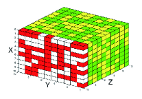
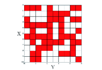
Figure 1: Each row in ‘X-Y’ dimension represents a tweet, in which each unit in a tweet is a word. In ‘X-Z’ dimension, each row represents a word vector. Red square represents that the word is positive related, otherwise it is white. The yellow square $i$ represents that the feature $i$ is positive related, otherwise it is green. Different tweets contain different words. Hence, the units in the same column on Y dimension probably represent different words.

Let a graph $G=(B,F)$ denote a user-user network, in which the edges represent the behaviors among users. These behaviors of users can be easily extracted from the raw data, and they play an important role in identifying the missing people tweets. However, our aim is to identify missing people tweet in this paper, but not users. Hence, it’s vital to build a tweet-tweet network, in which the edges represent the retweet and reply relationship among tweets. In this case, we can exploit the behaviors information to help solve the missing people tweet identification problem. In this paper, a simple algorithm is employed to convert the adjacency matrix of $G=(B,F)$ to the edge adjacency matrix of $H=(U,V)$, as shown in Figure 2. The main idea of conversion algorithm is that if two edges share the same start or end node, there is a link between them. It means that the tweets, which are retweeted or replied by the same user, probably have the same labels.

Figure 2: Reformulation of the user behavior network. The original network is represented as a user-user matrix. The converted network is represented as a tweet-tweet matrix.

With the given notations, we formally define the missing people related tweets identification problem as follows:
Given a set of users $B$ with their tweets with content information $x\in\mathbb{R}^{m\times\sum_{i=1}^{m}n_{i}\times k}$, network information $H=(U,V)$ and the label information $y\in\mathbb{R}^{m}$. We try to learn a classifier $\beta$ to automatically label the unknown tweets as missing people related or not.

3 The model

We first introduce how we model the textual content information and the network information, respectively. Then, a unified model is proposed to combine these two information.

3.1 Modeling Content Information

The most important task is to distinguish missing people tweets from other social media topics. The key idea is that missing people tweets contain more missing people related words. We propose the $r$-instance learning method to model the content information and find the top-$r$ missing people related words in each iteration. In multi-instance learning task, only positive samples contain positive instances. Different from multi-instance learning, both the missing people related (positive) tweets and irrelevant (negative) tweets contain positively related instances. Hence, it’s more challenging to solve the problem in our paper. The proposed r-instance learning model, which picks up $r$ positive related words in each iteration, can identify the missing people tweets by the proportion of missing people related words in each tweet. The main idea of how we construct the model is as follows:

One of the most widely used methods for classification is Logistic Regression, which is an efficient and interpretable model. The classifiers can be learned by minimizing the following cross-entropy error function instead of sum-of-squares for a classification problem. It leads to faster training as well as improved generalization:

(3.1) $$\begin{split}&J(\beta)=\sum_{i=1}^{m}log(h_{\beta}(x))\\ &s.t.\quad h_{\beta}(x)=({1+e^{-y<{\beta},x>}})^{-1}\end{split}$$

where $x$ is the content feature matrix of the training data and $\beta$ is the weight of features. The goal is to get the optimal $\beta$ in minimizing the loss function $J(\beta)$.

However, the content feature matrix $x\in\mathbb{R}^{m\times\sum_{i=1}^{m}n_{i}\times k}$ in our paper is a complex tensor. For each tweet $i$, the length of which $n_{i}$ is different from others. It makes the Logistic Regression unable to handle the complicated data. Hence, we add $u_{i}$ to evaluate the weights of words in each tweet $i$.

The following formulation is proposed to introduce parameter $u$ into the model:

(3.2) $$\begin{split}&h_{\beta,u}(x_{i})=({1+e^{-y_{i}<{\beta},x_{i}^{T}u_{i}>}})^{-1}\end{split}$$

The corresponding loss function is as follows:

(3.3) $$\begin{split}&J(\beta,u)=\sum_{i=1}^{m}log(h_{\beta,u}(x_{i}))\end{split}$$

where the parameter $\beta$ is to evaluate the importance of each feature dimension. In fact, not all words are missing people related. Hence, we intend to automatically select positive related words in each iteration and neglect the negatively related words. The $\ell_{0}$-norm is proposed to restrict the number of positive related words we select in each iteration. We get

(3.4) $$\begin{split}&J(\beta,u)=\sum_{i=1}^{m}log(h_{\beta,u}(x_{i}))\\ &\qquad\qquad s.t.\ ||u_{i}||_{0}\leq r,i=1,2,....,n\\ &\qquad\qquad\qquad h_{\beta,u}(x_{i})=({1+e^{y_{i}<{\beta},x_{i}^{T}u_{i}>}})^{-1}\end{split}$$

where parameter $\ell_{0}$-norm of $u_{i}$ is to substantially select missing people related words in tweet $i$. $r\in R$ is the constraint of a number of selected words in a single iteration.

To avoid overfitting and increase the generalization of the model, we add the $\ell_{2}$-norm penalization of $\beta$.

(3.5) $$\underset{\beta,u}{min}\ \sum_{i=1}^{m}log(h_{\beta,u}(x_{i}))+\frac{\lambda_{1}}{2}||\beta||_{2}$$

$$\qquad s.t.\ ||u_{i}||_{0}\leq r,i=1,2,....,n$$

However, high-dimensional feature space makes the computational task extremely difficult. As we know, sparse learning method has shown its effectiveness in many real-world applications such as [55] to handle the high-dimensional feature space. Hence, we propose to make use of the sparse learning for selecting the most effective features. Sparse learning methods [29] are widely used in many areas, such as the sparse latent semantic analysis and image retrieval. Another superiority of sparse learning methods is that they can generate a more efficient and interpretable model. A widely used regularized version of least squares is lasso (least absolute shrinkage and selection operator) [55]. Hence, we can further learn a classifier through solving the $\ell_{1}$-norm penalization:

(3.6) $$\underset{\beta,u}{min}\ \sum_{i=1}^{m}log(h_{\beta,u}(x_{i}))+\frac{\lambda_{1}}{2}||\beta||_{2}+\lambda_{2}||\beta||_{1}$$

$$\qquad s.t.\ ||u_{i}||_{0}\leq r,i=1,2,....,n$$

3.2 Modeling Network Information

It is vital to consider network information in solving the missing people problem, as missing people tweets contain the useful behavior network information. Meanwhile, this information cannot be obtained from pure content information. Several studies have utilized network information in solving real-world problems: influential users identification [46], recommendation [53] and topic detection [6]. It is indicated that the concept “homophily” is helpful for the classification, i.e. the vertices in the same community and the vertices connected with each other probably have similar labels. Motivated by these theories, we employ homophily and community structure to help identify the missing people tweets.

Many studies [43],[15] have been done to classify the vertices in networks. The vertice $u$’s in-degree is defined as $d^{in}_{u}=\sum_{[v,u]}{H(v,u)}$, and the vertice $u$’s out-degree is defined as $d^{out}_{u}=\sum_{[u,v]}{H(u,v)}$. $P$ is defined as the transition probability matrix of random walk in a graph with $P(u,v)=H(u,v)/d^{out}_{u}$. The stationary distribution $\pi$ of the random walk satisfies the following equation:

(3.7) $$\begin{split}\sum_{u\in V}{\pi(u)}=1,~{}~{}~{}\pi(v)=\sum_{[u,v]}{\pi(u)P(u,v)}.\end{split}$$

The network information is used to smooth the unified model. The classification problem can be formulated as minimizing

(3.8) $$R(f):=\frac{1}{2}\sum_{[u,v]\in E}{\pi(u)P(u,v)||\hat{Y_{u}}-\hat{Y_{v}}||^{2}},$$

where $\hat{Y_{u}}=\frac{f(u)}{\sqrt{\pi{(u)}}}$ is the predicted label of tweet $u$, and $\hat{Y_{v}}=\frac{f(v)}{\sqrt{\pi{(v)}}}$ is the predicted label of tweet $v$. $\mathcal{H}(V)$ is the function space, and $f\in\mathcal{H}(V)$ is the classification function, which assigns a label sign $f(v)$ to each vertex $v\in V$. If two tweets $u$ and $v$ are close to each other and have different predicted labels, the above loss function will have a penalty. For solving the Equation 3.8, we introduce an operator $\Theta:\mathcal{H}(V)\rightarrow\mathcal{H}(V)$.

(3.9) $$\begin{split}(\Theta f)(v)=&\frac{1}{2}\bigg{(}\sum_{u\rightarrow v}{\frac{\pi(u)P(u,v)f(u)}{\sqrt{\pi(u)\pi(v)}}}\\ &+\sum_{u\leftarrow v}{\frac{\pi(v)P(v,u)f(u)}{\sqrt{\pi(v)\pi(u)}}}\bigg{)}.\end{split}$$

It has been showed that the objective function can be interpreted by the following equation:

(3.10) $$R(f)=tr(\hat{Y}\mathcal{L}\hat{Y}^{T}),$$

where the $\mathcal{L}=I-\Theta$.

(3.11) $$\Theta=\frac{\Pi^{1/2}P\Pi^{-1/2}+\Pi^{-1/2}P^{T}\Pi^{1/2}}{2},$$

where $\Pi$ is a diagonal matrix with entries $\Pi(v,v)=\pi(v)$. $\pi$ denotes the eigenvector of the transition probability $P$, and $P^{T}$ is the transpose of $P$. If the original network is an undirected network, the $\mathcal{L}$ is reduced to $D-A$. $\mathcal{L}$ is symmetric and positive-semidefinite. $D$ is degree matrix and $A$ is adjacency matrix of the graph. Hence, the final objective function Equation 3.8 can be rewritten to the following formula:

(3.12) $$\begin{split}\frac{1}{2}||\beta^{T}(Xu)^{T}\mathcal{L}(Xu)\beta||\end{split}$$

3.3 Objective Function

Traditional text classification methods intend to add new features or propose effective classifiers to successfully solve the problem. On the one hand, the dimension of the text feature is always high. Traditional methods are not able to handle high dimension features. These methods have to select features first, and then learn a model to classify the texts. Sparse learning method, which can automatically select features and learn a model, is a good choice to solve the problem. On the other hand, network structure information plays an important role in the problem of missing people tweets identification. The homophily and community structure are used to formulate the behaviors among tweets. The behavior network contains much useful information that text information doesn’t have. Hence, we further integrate two kinds of features.

We propose to consider both network and content information in a unified model. By considering both network and content information, the missing people tweets recognition problem can be formulated as the optimization problem:

(3.13) $$\begin{split}&J(\beta,u)=\sum_{i=1}^{m}log(h_{\beta,u}(x_{i}))\\ &+\frac{\lambda_{1}}{2}||\beta||_{2}+\lambda_{2}||\beta||_{1}+\frac{\lambda_{3}}{2}||\beta^{T}(Xu)^{T}\mathcal{L}(Xu)\beta||\\ &\qquad s.t.\ ||u_{i}||_{0}\leq r,i=1,2,....,n\end{split}$$

3.4 The Optimization Algorithm

The objective function contains two parameters $\beta$ and $u_{i},\ i=1,2,...,m$. The exists of $u_{i}$ is a non-convex sparsity-inducing regularizer. Hence, it’s a highly non-convex and non-smooth optimization problem. Traditional gradient descent algorithm failed to find the optimal of the problem. Thus, we employ an iterative coordinate descent algorithm to efficiently solve the optimization problem. Take the $p=(\beta,u_{1},...,u_{m})$ as the parameter in each iteration. Then, the optimization problem is as follows:

(3.14) $$\begin{split}&\underset{p}{min}\ J(p)=f(p)+\sum_{i=1}^{m}r_{i}(p_{i})\end{split}$$

where $r_{i}(p_{i})=\frac{\lambda_{1}}{2}||\beta||_{2}+\lambda_{2}||\beta||_{1}$. The BCD method of Gauss-Seidel type iteration method [67] is adopted to iteratively update the the parameters. We make a prox-linear surrogate function to approximate the upper bound of the loss function $J(p^{k+1})$, and then each parameter $p$ can be updated as follows:

(3.15) $$\begin{split}p_{i}^{k+1}\in\ arg\ \underset{p_{i}}{min}&\ f_{i}^{k}(\hat{p}_{i}^{k+1})+<\hat{g}_{i}^{k},p_{i}-\hat{p_{i}}^{k+1}>\\ &+\frac{1}{2\alpha_{k}}||p_{i}-\hat{p_{i}}^{k+1}||_{2}+r_{i}(p_{i})\end{split}$$

where the $g_{i}$ is the gradient in each iteration and the $\alpha_{k}$ is the step size in each iteration. As the first item in the above equation is a constant. We can get the following formula:

(3.16) $$\begin{split}arg\ \underset{p_{i}}{min}<\hat{g}_{i}^{k},p_{i}-\hat{p_{i}}^{k+1}>+\frac{1}{2\alpha_{k}}||p_{i}-\hat{p_{i}}^{k+1}||_{2}+r_{i}(p_{i})\end{split}$$

where $\hat{p_{i}}^{k+1}=p_{i}^{k}+\eta_{k}(p_{i}^{k}-p_{i}^{k-1})$. Similar to the Nesterov’s accelerated gradient descent [36], the weight $\eta_{k}$ can be iteratively calculated, which can greatly speed up the convergence. And the proper step size $\alpha_{k}$ is calculated by the backtracking line search under the criterion:

(3.17) $$\begin{split}f(p^{k})\leq f(\hat{p}^{k-1})+<\bigtriangledown f_{i}^{k}(\hat{p}^{k-1}),p_{i}-\hat{p_{i}}^{k+1}>+\frac{L_{k}}{2}||p_{i}-\hat{p_{i}}^{k+1}||_{2}.\end{split}$$

where the $L_{k}$ is the Lipschitz constant, which is defined by the $\alpha_{k}=\frac{\xi}{L_{k}}$ with $\xi\in(0,1]$.

To optimize $\beta$, we fix $u_{i}$. The gradient of loss function is

(3.18) $$\begin{split}\bigtriangledown&J(\beta)=\sum_{i=1}^{m}({1+e^{-y_{i}(<\beta,x_{i}^{T}u_{i}>)}})^{-1}*e^{-y_{i}(<\beta,x_{i}^{T}u_{i}>)}\\ &*(-y_{i}(x_{i}^{T}u_{i}))+\lambda_{1}\beta+\lambda_{2}sign(\beta)+\lambda_{3}(Xu)^{T}\mathcal{L}(Xu)\beta\end{split}$$

The $\beta$ can be updated by the following eqation:

(3.19) $$\begin{split}\beta^{k+1}=\beta^{k}-\alpha_{k}\bigtriangledown J(\beta^{k})\end{split}$$

To optimize $u_{i}$, we keep the $\beta$ fixed. The gradient of the loss function is

(3.20) $$\begin{split}\bigtriangledown J(u_{i})=&({1+e^{-y_{i}<\beta,x_{i}^{T}u_{i}>}})^{-1}*e^{-y_{i}<\beta,x_{i}^{T}u_{i}>}\\ &*<\beta,x_{i}^{T}>+\lambda_{3}X^{T}\mathcal{L}Xu\beta\beta^{T}\end{split}$$

The $u_{i}$ can be updated by the following eqation:

(3.21) $$\begin{split}u_{i}^{k+1}=proj(u_{i}^{k}-\alpha_{k}\bigtriangledown J(u_{i}^{k}))\end{split}$$

where $proj$ is a projection operator with the constraint $||u_{i}||_{0}\leq r$. The optimization algorithm is shown in Algorithm 1. The convergence process is shown in Figure 3. Suppose the optimization algorithm takes $T$ iterations with $m$ samples, the overall time complexity is $O(Tm^{3}+Tm^{2})$ The loss of the objective function goes down shparply in the first 50 iterations. The subtle fluctuation of the line in the figure lies in the non-convex property of the objective function.

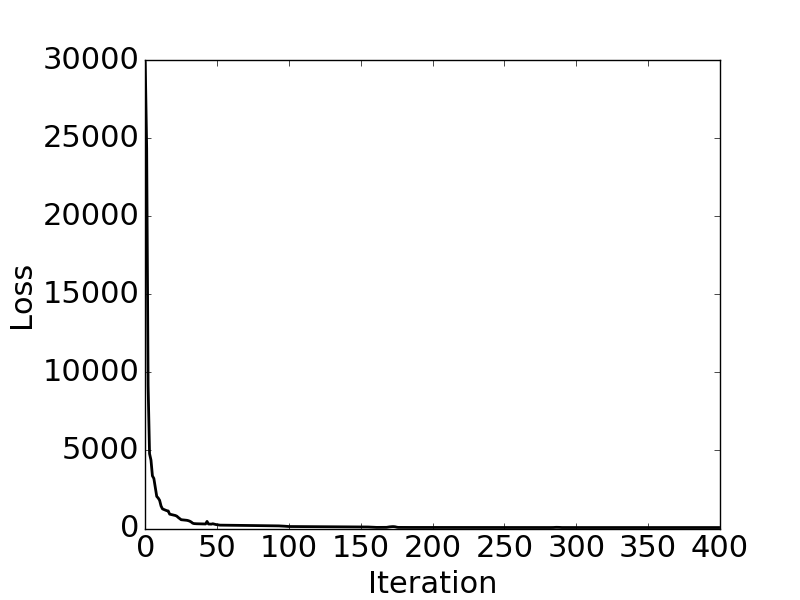
Figure 3: The convergence rate of the optimization algorithm.

Algorithm 1 The optimization algorithm for the unified objective function.

0:     The set of tweets text information: X The label of the tweets set: Y The Laplacian Matrix of tweets: L

0:     Parameter: $\beta$

  Initialize parameters $\beta$,$u_{i}$ and step size $\alpha_{k}$

  

  while it is not convergence do

       Compute the gradient of $\beta$ by Eq. 3.18

       Backtracking line search to identify the $\alpha_{k}$

       Update $\beta^{k+1}$ by Eq. 3.19

       for each sample $i$ in all tweets

         Compute the gradient of $u_{i}$ by Eq. 3.20

         Backtracking line search to identify the $\alpha_{k}$

         Update $u_{i}$ by Eq. 3.21

       end for

       $k=k+1$

  end while

4 Experiments

In this section, we introduce the dataset, and then give a case study of the missing people tweet. Then, we evaluate the effectiveness of the proposed method in this paper, and analyze the effectiveness of the network structure and content information. The experiments in this section focus on solving the following questions,

1. How effective is the proposed method compared with the baseline methods?

2. What are the effects of the network structure and content information?

4.1 Data Set

The real-world weibo data set used in our experiment is crawled from September 2014 to February 2015. We generally sampled a 40,373 tweets datasets with 1,404 positive samples, which contain keyword ‘missing people’. The positive ratio is 3.48%. Hence, we use the undersampling technique to iteratively update the parameters. 5 students annotate these data as positive and negative according to whether the tweet is looking for missing people.

Each tweet is retweeted or replied by 16.8 times on average. The retweet/reply frequencies follow the power law distribution, which indicates that few of the tweets draw much attention, as shown in Figure 4 , and most of the tweets are neglected by social media users.

Table 1: Summary of the Experimental Data set

Tweets	Positive ratio
40,373	3.48%
Users	Characteristic path length
40,579	5.878

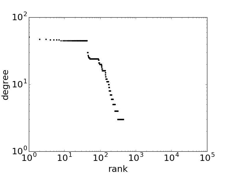
Figure 4: The degree distribution of the network. The degree distribution of the network fits the power law distribution. The vertices with 0 degree are omitted. And 20% of the tweets are retweeted or replied for 80% times.

4.2 Case study

The missing people tweets are shown in Table 2. The labels lie in the first column. The tweet content lies in the second column. We replace the name and HTTP link with #USERNAME# and #HTTP#, respectively. The topic hashtag of the tweet is deleted. The first tweet in the Table is a standard missing people tweet. It contains detailed information of the missing people: name, age, location, height, and so on. The second tweet is also a missing people tweet to find an old man with the Alzheimer’s disease. The third tweet is a missing person that post a tweet to find his parents. The fourth and fifth tweets are just complaints on social network. Traditional machine learning methods can successfully identify most of the missing people tweets except the second one in the table. The second tweet doesn’t contain any detailed information. However, it has a hyperlink which contains information of the missing people and it is retweeted by many commonweal organization users who ever retweeted missing people tweets. In our model, we introduce the behaviors of users by incorporating the Laplacian matrix into RI model. In this case, the parameter $\beta$ is greatly smoothed. It leads to increase the precision of the model but decrease the recall to some extent. That’s the reason why our model gets a good performance with a relatively balanced precision and recall.

Table 2: A case study of missing people tweets

Label	Tweet
1	#USERNAME# 10 yrs old, was last seen in Haidianat the swimming Pool. He approximately 5′0″, with light brown hair and a large birthmark on his right forearm. Last seen wearing jeans and either a white or red Nike shirt.
1	#USERNAME# with Alzheimer’s disease, was seen at 11am #HTTP#
1	I was born on sep 4 1989. Abandoned at Jingde, Jiangxi. Single eyelid. A birthmark on left side of her forehead. Height 167cm. Blood: O. Foster parents found me with a paper sticked to clothes.
0	Constantly hearing her mom talk about more people going missing or dead. It’s a terrifying thought.
0	I end up missing the people who did nothing but make me sad.

4.3 Experimental Setup

In particular, we apply different machine learning methods on the data set. Precision, recall and F1-measure are used as the performance metrics. F1 measure that combines precision and recall is the harmonic mean of precision and recall.

(4.22) $$F=2\cdot\frac{precision\cdot recall}{precision+recall}.$$

4.4 Feature Engineering

We analyze the data set according to the network structure and content, respectively. We discuss how we preprocess the texts and extract features from the texts first. Then, the homophily and modularity of the network are introduced to interpret the property of the network.

4.4.1 Preprocessing

The missing people related tweets are informative although they are noisy and sparse. We follow a standard process to remove stemming and stopwords first. Any user mentions processed by a “@” are replaced by the anonymized user name “USERNAME”. Any URLs starting with “Http” are replaced by the token “HTTP”. Emoticons, such as ‘:)’ or ‘T.T’, are also included as tokens.

4.4.2 Features

We investigate the tweets and propose domain-specific features. The linear combination of POS colored feature, tag based feature, morphological feature, NER feature, tweet length feature and Laplacian matrix is called general feature.

• Word2vec: It is a two-layer neural net that processes text. Its input is a text corpus and its output is a set of feature vectors for words in that corpus

• Word based features: Part-Of-Speech (POS) colored unigrams+bigrams. POS tagging is done by the Jieba package. When the corpus is large, the dimensions of the unigrams and unigram+bigrams features are too high for a PC to handle. Hence, we pick up the POS colored unigrams+bigrams feature.

• Tag based features: Most of the missing people tweets have tags. Having a tag in the tweet may promote more users reach the information.

• Morphological features: These include the feature each for frequencies of

  • the number in the sentence

  • the question mark in the sentence

  • the exclamation mark in the sentence

  • the quantifiers in the sentence

• NER features: Most of the positively related tweets contain the name, location, organization and time.

• Tweet features: the length of tweets

• Laplacian matrix: the structure information

4.4.3 Network Analysis

With the development of online social networks, social network analysis is introduced to solve many practical problems. Network analysis examines the structure of relationships among social entities. Since the 1970s, the empirical study of networks has played a central role in social science, and many of the mathematical and statistical tools are used for studying networks in sociology. In this part, we intend to employ the sociology theory and network analysis techniques to gradually analyze the network feature on the missing people information network.

A network is constructed based on the users’ behaviors on the data. An example is shown in Figure 5.

a) Vertices lying in a densely linked subgraph are likely to have the same labels. The modularity of the network is 0.84, which means that the network has a strong community structure. The figure shows that the red links are probably clustered in several communities. The bridges/spanners among communities are probably missing people tweets. The reason may lie in that the missing people tweets propagate further than normal tweets.

b) The nominal assortativity coefficient of the network is a way to specify the extent to which the connections stay within categories. Assuming that the edges belong to two different categories (missing people tweets or not), the following function calculates the assortativity coefficient $r$.

(4.23) $$r=\frac{\sum_{i}{e_{ii}-{\sum_{i}a_{i}b_{i}}}}{{1-\sum_{i}a_{i}b_{i}}}=\frac{Tr(e)-||e^{2}||}{1-||e^{2}||}.$$

where $e$ is the category matrix of the network and $||e^{2}||$ is the sum of all elements of the matrix $e^{2}$. $a_{i}$ and $b_{i}$ are labels.

On missing people tweets network, the assortativity coefficient is 0.422, which indicates that the similar edges are classified into the same class. More specifically, a pair of edges linked by a vertice are likely to have the same labels. As shown in Figure 5, almost all red/green edges (tweets) share the same starting or ending vertices. Hence, tweets in homophilic relationships share common characteristics, i.e. edges that have same starting or ending vertices have similar labels. Based on the above analysis, we find that social network structure information provides much useful information to help identify the missing people tweets.

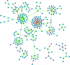
Figure 5: A typical structure of the missing people information network. The vertices represent tweets. The edges are replied/retweeted behaviors. If the tweet is missing people related, the edge is marked as green. Otherwise, it is red.

4.5 Performance Evaluation

Missing people tweets contain more missing people related words. The proposed method finds the top-r missing people related words in each iteration. When the optimal algorithm converges, the overall proportion of the missing people related words in each tweet identifies the label of the tweet. Hence, the prediction is to label the tweet as positive, if the tweet contains more missing people related words with threshold 0.6. Missing people related word $j$ in tweet $i$ is defined as $\sum{(\beta\times x_{ij})}\geq 0.9$.

Table 3: Performance on 40,373 tweets with word2vec features

Method	F1	Precision	Recall
SVM	0.849532	0.809052	0.896852
LR	0.843561	0.824009	0.868482
GNB	0.318648	0.194617	0.883459
SGD	0.849432	0.802560	0.879655
DT	0.794477	0.798115	0.787521
RF	0.795088	0.802738	0.792527
RIWN	0.814815	0.745020	0.899038
RI	0.863706	0.844311	0.884013

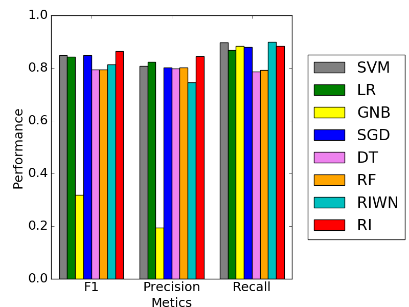
Figure 6: The performance of all models on the dataset.

We compare our proposed method with the baseline methods: SVM [52], Logistic Regression (LR) [16], Gaussian Naive Bayes (GNB) [21], SGD [64], Decision Tree (DT) [12, 45], Random Forests (RF) [26] and r-instance learning without network information (RIWN). According to the results in Table 3 and Figure 6, we can draw a conclusion that the RI model outperforms other methods in precision and F1-measure. Without network information, the RIWN model achieves a high recall, while the RI model achieves a relatively balanced precision and recall with network regularization. Most of these methods have a high recall and low precision. Compared with the RIWN, the network information greatly smooths the parameters in RI model, and make the RI model get a relatively balanced precision and recall. The performance of SGD is not as good as that of SVM. The reason is that the poor performance of L2 regularization is linked to rotational invariance. GaussianNB method has a small precision value on both word2vec and general features, which results in wrongly identifying some of the positive tweets. GaussianNB, which is a non-linear model, is really not a good estimator for text classification task.

To compare the performance of the word2vec and general features on many traditional machine learning methods, we use the remaining features (exluding word2vec) on the baseline methods. The results are shown in Tables 3 and 4. In Table 3, we apply word2vec features on many traditional methods. The feature of tweet $i$ is a linear combination of each word vector in tweet $i$. In Table 4, we apply traditional machine learning methods on the general feature. As shown in Tables 3 and 4, word2vec feature outperforms the combination of domain-specific features in almost all models.

Table 4: Performance on 40,373 tweets with general features.

Method	F1	Precision	Recall
SVM	0.794475	0.813730	0.776212
LR	0.787828	0.831698	0.758183
GNB	0.579885	0.504899	0.791644
SGD	0.747827	0.725033	0.702323
DT	0.825986	0.823979	0.824728
RF	0.828921	0.823824	0.826044

The performance of all the methods cannot solve the classification problem perfectly. The reasons are as follows: (1) Though we provide instructions for annotators, some tweets are so ambiguous that they cannot distinguish the class of the tweet. For instance, some tweets with a hyperlink contain only 2 words–“missing people”. The information is too limited to judge whether it is a spam or not.

(2) Some tweets search an unfamiliar charming boy/girl that the user met by accident in the real world. It’s a “searching” people tweet. And the feature of this kind of tweet is similar to the missing people “missing people” related tweets. Annotators have different criterions. They mark these tweets as different marks.

4.6 Parameter Analysis

In this section, we will further explore the values of the parameters in the RI model. $\lambda_{1}$ is responsible for avoiding overfitting. $\lambda_{2}$ is responsible for controlling the sparseness of the selected feature and model. $\lambda_{3}$ is responsible for balancing the importance of the content and social network information to the model. $\lambda_{1}$ is empirically set to 0.002, $\lambda_{2}$ is set to 0.1, and $\lambda_{3}$ is set to 0.2. The restictions on the $\ell_{0}$-norm on $u_{i}$ is set to 50.

4.7 The Effectiveness of the Proposed Method

We use t-test to justify the effectiveness of our method with the SVM. According to the experimental results, we can get two groups of F1-values for the proposed method and Logistic Regression.The corresponding F-values are $\bar{F}_{t}$ and $\bar{F}_{l}$. The null hypothesis is that there is no significant difference between the two groups of F1-values, $H_{0}:\mathit{\bar{F}}_{t}=\mathit{\bar{F}}_{l}$; while the alternative hypothesis is the mean F-value of the proposed method is larger than that of Logistic Regression, as shown in Equation $H_{0}:\mathit{\bar{F}}_{t}=\mathit{\bar{F}}_{l},\ H_{1}:\mathit{\bar{F}}_{t}>\mathit{\bar{F}}_{l}$. The null hypothesis is rejected at the significant level $\alpha=0.05$.

The t-test results show that the observation value is 68.352, and p-value is 0.00, which is less than the significance level. Hence, the variances of two groups of F1-values have significant differences. The results of other methods are similar, which proves the effectiveness of RI model.

5 Conclusions

The word embedding features and social theories provide a good chance to help identify and analyze the missing people tweets. We employ both the content and network information to perform effective missing people tweets recognition. The RI model in this paper combines the content and network information into a unified model. We also propose an efficient algorithm to solve the non-smooth convex optimization problem. The experimental results on a real weibo data set indicate that RI model can effectively detect missing people tweets, and outperform the alternative supervised learning methods.

References

- [1] Rutvica Andrijasevic. Beautiful dead bodies: gender, migration and representation in anti-trafficking campaigns. feminist review, 86(1):24–44, 2007.
- [2] Christopher Anton. Adverse drug reactions and social media. Adverse Drug Reaction Bulletin, 286(1):1103–1106, 2014.
- [3] Francis R Bach and Michael I Jordan. Kernel independent component analysis. The Journal of Machine Learning Research, 3:1–48, 2003.
- [4] Samy Bengio, Fernando Pereira, Yoram Singer, and Dennis Strelow. Group sparse coding. In Advances in Neural Information Processing Systems, pages 82–89, 2009.
- [5] Xi Chen, Weike Pan, James T Kwok, and Jaime G Carbonell. Accelerated gradient method for multi-task sparse learning problem. In Ninth IEEE International Conference on Data Mining, pages 746–751. IEEE, 2009.
- [6] Yan Chen, Zhoujun Li, Liqiang Nie, Xia Hu, Xiangyu Wang, Tat-Seng Chua, and Xiaoming Zhang. A semi-supervised bayesian network model for microblog topic classification. In Proceedings of the 24th International Conference on Computational Linguistics, 2012.
- [7] Yilun Chen, Yuantao Gu, and Alfred O Hero. Regularized least-mean-square algorithms. arXiv preprint arXiv:1012.5066, 2010.
- [8] Fan Chung. Laplacians and the cheeger inequality for directed graphs. Annals of Combinatorics, 9(1):1–19, 2005.
- [9] Mike Dottridge. Trafficking in children in west and central africa. Gender & Development, 10(1):38–42, 2002.
- [10] Ender M Eksioglu. Group sparse rls algorithms. International Journal of Adaptive Control and Signal Processing, 28(12):1398–1412, 2014.
- [11] Xiao Feng, Yang Shen, Chengyong Liu, Wei Liang, and Shuwu Zhang. Chinese short text classification based on domain knowledge. In International Joint Conference on Natural Language Processing, pages 859–863, 2013.
- [12] Mark A Friedl and Carla E Brodley. Decision tree classification of land cover from remotely sensed data. Remote Sensing of Environment, 61(3):399–409, 1997.
- [13] Jerome Friedman, Trevor Hastie, and Robert Tibshirani. A note on the group lasso and a sparse group lasso. arXiv preprint arXiv:1001.0736, 2010.
- [14] Oren Glickman, Ido Dagan, and Moshe Koppel. A probabilistic classification approach for lexical textual entailment. In Twentieth National Conference on Artificial Intelligence (AAAI, 2005.
- [15] Matthew Hansen, R Dubayah, and R DeFries. Classification trees: an alternative to traditional land cover classifiers. International Journal of Remote Sensing, 17(5):1075–1081, 1996.
- [16] David W Hosmer Jr and Stanley Lemeshow. Applied Logistic Regression. John Wiley & Sons, 2004.
- [17] Xia Hu and Huan Liu. Text analytics in social media. In Mining text data, pages 385–414. Springer, 2012.
- [18] ILO-IPEC. Child trafficking - essentials. 2010.
- [19] Keyuan Jiang and Yujing Zheng. Mining twitter data for potential drug effects. In Advanced Data Mining and Applications, pages 434–443. Springer, 2013.
- [20] Thorsten Joachims. Making large scale svm learning practical. Technical report, Universität Dortmund, 1999.
- [21] George H John and Pat Langley. Estimating continuous distributions in bayesian classifiers. In Proceedings of the Eleventh Conference on Uncertainty in Artificial Intelligence, pages 338–345. Morgan Kaufmann Publishers Inc., 1995.
- [22] A Jordan. On discriminative vs. generative classifiers: A comparison of logistic regression and naive bayes. Advances in neural information processing systems, 14:841, 2002.
- [23] Jihie Kim and Jaebong Yoo. Role of sentiment in message propagation: Reply vs. retweet behavior in political communication. In Social Informatics (SocialInformatics), 2012 International Conference on, pages 131–136. IEEE, 2012.
- [24] Kwanho Kim, Beom-suk Chung, Yerim Choi, Seungjun Lee, Jae-Yoon Jung, and Jonghun Park. Language independent semantic kernels for short-text classification. Expert Systems with Applications, 41(2):735–743, 2014.
- [25] Charles L Lawson and Richard J Hanson. Solving least squares problems, volume 161. SIAM, 1974.
- [26] Andy Liaw and Matthew Wiener. Classification and regression by randomforest. R News, 2(3):18–22, 2002.
- [27] J. Liu, S. Ji, and J. Ye. SLEP: Sparse Learning with Efficient Projections. Arizona State University, 2009.
- [28] Jun Liu, Shuiwang Ji, and Jieping Ye. Multi-task feature learning via efficient l 2, 1-norm minimization. In Proceedings of the twenty-fifth conference on uncertainty in artificial intelligence, pages 339–348. AUAI Press, 2009.
- [29] Jun Liu, Shuiwang Ji, and Jieping Ye. Slep: Sparse learning with efficient projections. Arizona State University, 6:491, 2009.
- [30] Jun Liu and Jieping Ye. Fast overlapping group lasso. arXiv preprint arXiv:1009.0306, 2010.
- [31] Tao Liu, Xiaoyong Du, Yongdong Xu, Minghui Li, and Xiaolong Wang. Partially supervised text classification with multi-level examples. Twenty-Fifth AAAI Conference on Artificial Intelligence, 2011.
- [32] Qing Lu and Lise Getoor. Link-based Text Classification. In International Joint Conference on Artificial Intelligence.
- [33] Craig McGill. Human traffic sex, slaves and immigration. Vision Paperbacks, 2003.
- [34] Scott Menard. Applied Logistic Regression analysis, volume 106. Sage, 2002.
- [35] Tomas Mikolov, Kai Chen, Greg Corrado, and Jeffrey Dean. word2vec. 2014.
- [36] Yurii Nesterov. A method of solving a convex programming problem with convergence rate o (1/k2). In Soviet Mathematics Doklady, volume 27, pages 372–376, 1983.
- [37] Yurii Nesterov. Introductory lectures on convex optimization, volume 87. Springer Science & Business Media, 2004.
- [38] Mark Newman. Networks: an introduction. Oxford University Press, 2010.
- [39] Feiping Nie, Heng Huang, Xiao Cai, and Chris H Ding. Efficient and robust feature selection via joint l2, 1-norms minimization. In Advances in Neural Information Processing Systems, pages 1813–1821, 2010.
- [40] Kamal Nigam, Andrew Kachites McCallum, Sebastian Thrun, and Tom Mitchell. Text classification from labeled and unlabeled documents using em. Machine learning, 39(2-3):103–134, 2000.
- [41] Elaine Pearson. Human traffic, human rights: Redefining victim protection. Anti-Slavery International, 2002.
- [42] Xuan-Hieu Phan, Le-Minh Nguyen, and Susumu Horiguchi. Learning to classify short and sparse text & web with hidden topics from large-scale data collections. In Proceedings of the 17th international conference on World Wide Web, pages 91–100. ACM, 2008.
- [43] John C Platt, Nello Cristianini, and John Shawe-Taylor. Large margin dags for multiclass classification. In Advances in Neural Information Processing Systems 12, volume 12, pages 547–553, 1999.
- [44] Qiang Pu and Guo-Wei Yang. Short-text classification based on ica and lsa. In International Symposium on Neural Networks, pages 265–270. Springer, 2006.
- [45] J. Ross Quinlan. Generating Production Rules from Decision Trees. In International Joint Conference on Artificial Intelligence, pages 304–307, 1987.
- [46] Roshan Rabade, Nishchol Mishra, and Sanjeev Sharma. Survey of influential user identification techniques in online social networks. In Recent Advances in Intelligent Informatics, pages 359–370. Springer, 2014.
- [47] Radim Řehůřek and Petr Sojka. Software framework for topic modelling with large corpora. In Proceedings of the LREC 2010 Workshop on New Challenges for NLP Frameworks, pages 45–50. ELRA, May 2010.
- [48] Shari Kessel Schneider, Lydia O’Donnell, Ann Stueve, and Robert WS Coulter. Cyberbullying, school bullying, and psychological distress: A regional census of high school students. American Journal of Public Health, 102(1):171–177, 2012.
- [49] Louise Shelley and M Lee. Human trafficking as a form of transnational crime. Human trafficking, pages 116–137, 2007.
- [50] Bharath Sriram, Dave Fuhry, Engin Demir, Hakan Ferhatosmanoglu, and Murat Demirbas. Short text classification in twitter to improve information filtering. In Proceedings of the 33rd international ACM SIGIR conference on Research and development in information retrieval, pages 841–842. ACM, 2010.
- [51] Aixin Sun. Short text classification using very few words. In Proceedings of the 35th international ACM SIGIR conference on Research and development in information retrieval, pages 1145–1146. ACM, 2012.
- [52] Johan AK Suykens and Joos Vandewalle. Least squares support vector machine classifiers. Neural Processing Letters, 9(3):293–300, 1999.
- [53] Jiliang Tang, Xia Hu, and Huan Liu. Social recommendation: a review. Social Network Analysis and Mining, 3(4):1113–1133, 2013.
- [54] David TAPP and Susan JENKINSON. Trafficking of children. Criminal Law and Justice Weekly, 177(9):134–136, 2013.
- [55] Robert Tibshirani. Regression shrinkage and selection via the lasso. Journal of the Royal Statistical Society. Series B (Methodological), pages 267–288, 1996.
- [56] Bing-kun Wang, Yong-feng Huang, Wan-xia Yang, and Xing Li. Short text classification based on strong feature thesaurus. Journal of Zhejiang University SCIENCE C, 13(9):649–659, 2012.
- [57] Jie Wang and Jieping Ye. Two-layer feature reduction for sparse-group lasso via decomposition of convex sets. In Advances in Neural Information Processing Systems, pages 2132–2140, 2014.
- [58] Senzhang Wang, Xia Hu, Philip S. Yu, and Zhoujun Li. Mmrate: Inferring multi-aspect diffusion networks with multi-pattern cascades. In KDD, 2014.
- [59] Stanley Wasserman. Social network analysis: Methods and applications, volume 8. Cambridge university press, 1994.
- [60] Melanie Grayce West. Pooling resources to fight child abuse and abduction. 2012.
- [61] Phil Williams. Trafficking in women and children: A market perspective. Transnational Organized Crime, 3(4):145–171, 1997.
- [62] Diane K Wysowski and Lynette Swartz. Adverse drug event surveillance and drug withdrawals in the united states, 1969-2002: the importance of reporting suspected reactions. Archives of internal medicine, 165(12):1363–1369, 2005.
- [63] Shuo Xiang, Xiaotong Shen, and Jieping Ye. Efficient nonconvex sparse group feature selection via continuous and discrete optimization. Artificial Intelligence, 2015.
- [64] Lin Xiao. Dual averaging method for regularized stochastic learning and online optimization. In Advances in Neural Information Processing Systems, pages 2116–2124, 2009.
- [65] Jun-Ming Xu, Kwang-Sung Jun, Xiaojin Zhu, and Amy Bellmore. Learning from bullying traces in social media. In Proceedings of the 2012 conference of the North American chapter of the association for computational linguistics: Human language technologies, pages 656–666. Association for Computational Linguistics, 2012.
- [66] Jun-Ming Xu, Xiaojin Zhu, and Amy Bellmore. Fast learning for sentiment analysis on bullying. In Proceedings of the First International Workshop on Issues of Sentiment Discovery and Opinion Mining, page 10. ACM, 2012.
- [67] Yangyang Xu and Wotao Yin. A globally convergent algorithm for nonconvex optimization based on block coordinate update. arXiv preprint arXiv:1410.1386, 2014.
- [68] Rui YAN, Xian-bin CAO, and Kai LI. Dynamic assembly classification algorithm for short text. Acta Electronica Sinica, 37(5):1019–1024, 2009.
- [69] Yi Yang, Heng Tao Shen, Zhigang Ma, Zi Huang, and Xiaofang Zhou. l2,1-norm regularized discriminative feature selection for unsupervised learning. In IJCAI Proceedings-International Joint Conference on Artificial Intelligence, volume 22, page 1589. Citeseer, 2011.
- [70] Lei Yuan, Jun Liu, and Jieping Ye. Efficient methods for overlapping group Lasso. In Advances in Neural Information Processing Systems, pages 352–360, 2011.
- [71] Sarah Zelikovitz. Using background knowledge to improve text classification. PhD thesis, Rutgers, The State University of New Jersey, 2002.
- [72] Sarah Zelikovitz and Haym Hirsh. Improving short text classification using unlabeled background knowledge to assess document similarity. In Proceedings of the seventeenth international conference on machine learning, volume 2000, pages 1183–1190, 2000.
- [73] Sarah Zelikovitz and Finella Marquez. Transductive learning for short-text classification problems using latent semantic indexing. International Journal of Pattern Recognition and Artificial Intelligence, 19(02):143–163, 2005.
- [74] Harry Zhang. The optimality of naive bayes. AA, 1(2):3, 2004.
- [75] Dengyong Zhou, Jiayuan Huang, and Bernhard Schölkopf. Learning from labeled and unlabeled data on a directed graph. In Proceedings of the 22nd International Conference on Machine Learning, pages 1036–1043. ACM, 2005.
- [76] Hui Zou and Trevor Hastie. Regularization and variable selection via the elastic net. Journal of the Royal Statistical Society: Series B (Statistical Methodology), 67(2):301–320, 2005.