Tunable coupling between a superconducting resonator and an artificial atom

Abstract

Coherent manipulation of a quantum system is one of the main themes in current physics researches. In this work, we design a circuit QED system with a tunable coupling between an artificial atom and a superconducting resonator while keeping the cavity frequency and the atomic frequency invariant. By controlling the time dependence of the external magnetic flux, we show that it is possible to tune the interaction from the extremely weak coupling regime to the ultrastrong coupling one. Using the quantum perturbation theory, we obtain the coupling strength as a function of the external magnetic flux. In order to show its reliability in the fields of quantum simulation and quantum computing, we study its sensitivity to noises.

I Introduction

The light-matter interaction in circuit quantum electrodynamics (QED) finds lots of applications in many quantum information processes, such as the simulation of resonance fluorescence Toyli et al. (2016), an experimental proposal for boson sampling Borja Peropadre and Aspuru-Guzik (2016) and the single-photon scattering on an atom Zhou et al. (2008); He et al. (2017); Forn-Díaz et al. (2017). All these achievements show that circuit QED is an excellent platform for studying the physics induced by light-matter interaction Forndiaz et al. (2010); Forn-Díaz et al. (2017); Gu et al. (2017); Yoshihara et al. (2017).

In previous studies, the photon-photon interaction Peropadre et al. (2013a); Baust et al. (2015); Wulschner et al. (2016) and the atom-atom interaction Kim (2006) have been investigated with elaborate superconducting Josephson junction circuits, and the photon-atom interaction has been studied in all coupling regimes. Nevertheless, we note that it is rarely mentioned how to control the light-matter interaction during an adiabatic process Tong et al. (2007), which is inevitable and valuable in such experiments. To this end, it becomes an urgent need to design a superconducting circuit for implementing the light-atom interaction with a continuously tunable coupling strength and with a fixed qubit frequency.

Designing such a circuit is equivalent to devising an unusual qubit. The widely used superconducting qubits includes phase qubit Martinis et al. (2005), transmon Koch et al. (2007), and Xmon Barends et al. (2013), which are different assemblies of Josephson junctions and other circuit components like capacitance, inductance. Because of different structures of these qubits, they can be manipulated by different external signals and sensitive to diverse noise sources. In the circuit QED, the single mode cavity can be realized by a LC oscillator or a microwave transmission line. To construct a quantum network, we need to couple qubits and photons, which can be implemented by the capacitance connection Inomata et al. (2012), the mutual inductance Mariantoni et al. (2008); van den Brink et al. (2005) and the direct connection Peropadre et al. (2010). In particular, it is worthy to point out that the direct connection between a qubit and a microwave transmission line has led the coupling strength into the ultrastrong regime Peropadre et al. (2010); Forn-Díaz et al. (2017).

Up to now, the qubit-resonator coupling strength can be tuned from zero to a finite value Gambetta et al. (2011); Srinivasan et al. (2011); Bruschi et al. (2013); Mezzacapo et al. (2014). This coupling strength is controlled by the direct capacitance between the upper island and the lower island, which can’t be tuned in time. Other than directly changing the capacitance, the external signals like magnetic flux can also be used to modify the photon-atom interaction. In general, the qubit frequency will be changed with the variation of the coupling strength Forn-Díaz et al. (2017). If we ignore the tiny variation of the qubit frequency, the dc-SQUID can be used as a tunable coupler to modulate the coupling strength Lu et al. (2017). However, the coupling strength controlled by this circuit design cannot be tuned in all coupling regimes.

Inspired by Refs. Inomata et al. (2012) and Peropadre et al. (2010), we devise an artificial atom based on the superconducting loop containing two dc-SQUIDs and make the photon-atom coupling flux-controlled. To see clearly the underlying mechanism, we theoretically calculate the coupling strength between two coupled states. As an application, we investigate the adiabatic dynamics of the qubit in superconducting resonators in all coupling regimes. Furthermore, we discuss the influence of the resistance of Josephson junctions on our circuit and show its extensive applicability in quantum simulations. For example, our system allows the adiabatic switching of the coupling strength from the strong to the ultra strong coupling regime which makes it a reliable tool for implementing a quantum memory Kyaw et al. (2015). Moreover, if fast-tuning is possible, our system can also be used for simulating the relativistic effects Felicetti et al. (2015); Garciaalvarez et al. (2017).

The rest of this paper is organized as follows. In Sec. II, after introducing our design, we analytically study the Hamiltonian of the artificial atom. With the help of quantum perturbation theory, we obtain the explicit formula of the coupling strength and the energy difference between two lowest eigenstates of the atom, which are detailed derived in Appendix A. Based on the formula, we propose the tunable coupling scheme, which makes our system a tunable coupling Rabi model. To test the experimental feasibility of our circuit, we consider the dissipation of the artificial atom in Sec. III. With all these analytical results, we estimate the proper value of device parameters of our qubit in a circuit QED experiment in Sec. IV. In Sec. V, we draw the conclusions.

II Tunable coupling

In this section, we study the mechanism for the coupling between an artificial atom and the superconducting resonator. The artificial atom is based on superconducting quantum interference devices (SQUIDs), which are widely used in circuit QED. To manipulate the energy splitting of the system as well as the coupling strength with outsides, we control three time-dependent magnetic fluxes. Since the coupling strength need to be tuned into the ultrastrong regime, we directly connect the atom to the transmission line. Based on the two previous ideas, we theoretically design the artificial atom schematically shown in Fig. 1. We will give its Hamiltonian and derive the expression for the coupling strength.

II.1 System Hamiltonian

Figure 1: (Color online). The schematic of the circuit layout of an artificial atom sharing an inductance with a coplanar transmission line. In the lumped element approximation, this transmission line resonator is constructed by two LC oscillators with the inductance $L_{0}$ and capacitance $C_{0}$. The artificial atom in the dashed gray rectangle is composed of a superconducting loop with two dc-SQUIDs. $C_{J}$ represents the capacitance of every Josephson junction. Three external magnetic fluxes are denoted as $\Phi_{1},\Phi_{2}$ and $\Phi_{3}$. $\phi^{a(b)}_{\rm{L}}$ and $\phi^{a(b)}_{\rm{R}}$ are the reduced node flux for each side of the LC resonator.

In Fig. 1, an artificial atom is galvanically attached to the center of the coplanar waveguide transmission line resonator which is described as a two-mode LC resonator with its inductance $L_{0}$ and capacitance $C_{0}$. As shown in the dashed gray rectangle of Fig. 1, this atom contains four Josephson junctions that are designed with the same area and combined into two dc-SQUIDs. Similar to the flux qubit, our atom adopts a superconducting coil to connect dc-SQUIDs in series. In order to eliminate the induced currents flowing to the connecting loop with self-inductance $L_{r}$, the penetrating fluxes of the two dc-SQUIDs have the same value ($\Phi_{1}=\Phi_{2}$) but are in opposite directions.

For simplicity, we neglect the additional flux generated by the circulating loop current in the dc-SQUIDs, which is equivalent to restricting our discussion to the screening parameter $\beta_{L}=\dfrac{L_{S}I_{c}}{\varphi_{0}}\ll 1$. Here, $L_{S}$ is the loop inductance of the dc-SQUID, $I_{c}$ is the critical current of the Josephson junctions, and $\varphi_{0}=\dfrac{\hbar}{2e}$ is the reduced flux quantum.

As shown in Fig. 1, we divide the system into two parts: the circuits inside and those outside of the dashed rectangle. The Lagrangian of our system is

$$\hat{L}=\hat{L}^{\prime}+\hat{L}^{\prime\prime}$$ (1)

with

$$\hat{L}^{\prime}=\sum^{4}_{i=1}\left[\dfrac{1}{2}C_{J}\varphi^{2}_{0}\dot{\phi}^{2}_{i}-E_{J}(1-\cos\phi_{i})\right]-\varphi_{0}^{2}\dfrac{(\phi^{b}_{\rm{L}}-\phi^{a}_{\rm{R}})^{2}}{2L_{r}},$$ (2a)

$$\hat{L}^{\prime\prime}=\dfrac{C_{0}}{2}\varphi^{2}_{0}[(\dot{\phi}^{a}_{\rm{L}})^{2}+(\dot{\phi}^{b}_{\rm{R}})^{2}]-\varphi^{2}_{0}\dfrac{(\phi^{a}_{\rm{L}}-\phi^{a}_{\rm{R}})^{2}+(\phi^{b}_{\rm{L}}-\phi^{b}_{\rm{R}})^{2}}{2L_{0}},$$ (2b)

where $L^{\prime}$ and $L^{\prime\prime}$ are the Lagrangian of the inside part and that of the outside part respectively, $\phi_{i}~{}(i=1,2,3,4)$ is the phase difference across the $i$-th junction, and $\phi^{a(b)}_{\rm{L(R)}}=\dfrac{1}{\varphi_{0}}\int^{t}_{-\infty}V^{a(b)}_{\rm{L(R)}}(\tau)d\tau$ is the reduced node flux Devoret (1995) which corresponds to the electric potential $V^{a(b)}_{\rm{L(R)}}$ for each side of the LC resonator.

Following Ref. Peropadre et al. (2010, 2013b), we introduce $\varphi_{\pm}=\phi^{b}_{\rm{R}}\pm\phi^{a}_{\rm{L}}$, $\Phi_{+}=\phi^{b}_{\rm{L}}+\phi^{a}_{\rm{R}}$ and consider $\phi_{r}=\phi^{b}_{\rm{L}}-\phi^{a}_{\rm{R}}$, then we rewrite the Lagrangian (2a) and (2b) into

$$\hat{L}^{\prime}=\sum^{4}_{i=1}\left[\dfrac{1}{2}C_{J}\varphi^{2}_{0}\dot{\phi}^{2}_{i}-E_{J}(1-\cos\phi_{i})\right]-\varphi_{0}^{2}\dfrac{\phi_{r}^{2}}{2L_{r}},$$ (3a)

$$\hat{L}^{\prime\prime}=\dfrac{C_{0}}{4}\varphi^{2}_{0}(\dot{\varphi}^{2}_{+}+\dot{\varphi}^{2}_{-})-\varphi^{2}_{0}\dfrac{(\varphi_{+}-\Phi_{+})^{2}+(\varphi_{-}-\phi_{r})^{2}}{4L_{0}}.$$ (3b)

Note that the conditions of fluxoid quantization along the independent loops in the circuit are given by

$$\phi_{2}-\phi_{1}=f,$$ (4a)

$$\phi_{3}-\phi_{4}=f,$$ (4b)

$$\phi_{2}+\phi_{4}-\phi_{r}=f^{\prime},$$ (4c)

where

$$f=\dfrac{\Phi_{1}}{\varphi_{0}}=\dfrac{\Phi_{2}}{\varphi_{0}},$$ (5a)

$$f^{\prime}=\dfrac{\Phi_{3}}{\varphi_{0}}.$$ (5b)

With the Lagrangian (3) and the relation (4), we write the Hamiltonian of our system

$$\begin{split}&\hat{H}^{\prime}=\dfrac{\Omega^{2}_{J}p^{2}_{+}}{8\hbar\omega_{r}}+\dfrac{\Omega^{2}_{J}p^{2}_{-}}{8\hbar\omega_{r}}+2\hbar\omega_{r}\phi^{2}_{+}+2E_{J}\left\{2-\cos\dfrac{f}{2}\right.\\ &\left.\times\left[\cos(\phi_{+}+\phi_{-}-\dfrac{f-f^{\prime}}{2})+\cos(\phi_{+}-\phi_{-}+\dfrac{f+f^{\prime}}{2})\right]\right\},\end{split}$$ (6)

and

$$\begin{split}\hat{H}^{\prime\prime}=&\dfrac{\omega^{2}_{c}p^{\prime 2}_{+}}{\hbar\omega_{0}}+\dfrac{\hbar\omega_{0}\varphi^{2}_{+}}{4}+\dfrac{\hbar\omega_{0}\Phi^{2}_{+}}{4}-\dfrac{\hbar\omega_{0}}{2}\varphi_{+}\Phi_{+}\\ &+\dfrac{\omega^{2}_{c}p^{\prime 2}_{-}}{\hbar\omega_{0}}+\dfrac{\hbar\omega_{0}\varphi^{2}_{-}}{4}+\hbar\omega_{0}\phi^{2}_{+}-\hbar\omega_{0}\varphi_{-}\phi_{+},\end{split}$$ (7)

where $\Omega_{J}=\dfrac{1}{\sqrt{L_{r}C_{J}}}$, $\hbar\omega_{r}=\dfrac{\varphi^{2}_{0}}{L_{r}}$, $\omega_{c}=\dfrac{1}{\sqrt{L_{0}C_{0}}}$, $\hbar\omega_{0}=\dfrac{\varphi^{2}_{0}}{L_{0}}$, and $p_{\pm}=4C_{J}\varphi^{2}_{0}\dot{\phi}_{\pm}$ is the conjugate momentum with corresponding phase difference $\phi_{\pm}=\dfrac{(\phi_{2}-f^{\prime}/2)\pm(\phi_{4}-f^{\prime}/2)}{2}$, $p^{\prime}_{\pm}=\dfrac{1}{2}C_{0}\varphi^{2}_{0}\dot{\varphi}_{\pm}$ is the canonical momentum which corresponds to $\varphi_{\pm}$.

From Eqs. (6) and (7), we can indicate that $\hat{H}^{\prime}$ represents the Hamiltonian of the artificial atom without outside connections, $\hat{H}^{\prime\prime}$ describes the two-mode LC resonator with intrinsic frequency $\omega_{c}$. Since $\phi_{+}$ forms the part of the qubit while $\Phi_{+}$ does not, we conclude that the qubit only couples with one mode of the resonator and $-\hbar\omega_{0}\varphi_{-}\phi_{+}$ represents the qubit-resonator interaction. In this sense, we can treat the circuit shown in Fig. 1 as a coupling system with one atom and a single-mode cavity. In this simplified system, the atomic Hamiltonian should consider not only the inside part of the dashed rectangle but also the renormalization $\hbar\omega_{0}\phi^{2}_{+}$ from outsides. Then the Hamiltonian of our system is

$$\hat{H}=\hat{H}_{\rm{atom}}+\hat{H}_{\rm{cav}}+\hat{H}_{\rm{int}},$$ (8)

where

$$\hat{H}_{\rm{atom}}=\hat{H}^{\prime}+\hbar\omega_{0}\phi^{2}_{+},$$ (9a)

$$\hat{H}_{\rm{cav}}=\dfrac{\omega^{2}_{c}p^{\prime 2}_{-}}{\hbar\omega_{0}}+\dfrac{\hbar\omega_{0}\varphi^{2}_{-}}{4},$$ (9b)

$$\hat{H}_{\rm{int}}=-\hbar\omega_{0}\varphi_{-}\phi_{+}.$$ (9c)

In the second quantization representation, the cavity Hamiltonian (9b) is rewritten as

$$\hat{H}_{\rm{cav}}=(\hat{a}^{\dagger}\hat{a}+\dfrac{1}{2})\hbar\omega_{c},$$ (10)

where $\hat{a}=\sqrt{\dfrac{\omega_{0}}{4\omega_{c}}}\left(\hat{\varphi}_{-}+\dfrac{2i\omega_{c}}{\hbar\omega_{0}}\hat{p}^{\prime}_{-}\right)$ is the photon annihilation operator for the cavity. Then the interaction Hamiltonian (9c) can be changed to

$$\hat{H}_{\rm{int}}=-\hbar\sqrt{\omega_{0}\omega_{c}}\phi_{+}(\hat{a}^{\dagger}+\hat{a}),$$ (11)

which implies that the tunable coupling to the cavity is mainly determined by $\phi_{+}$.

II.2 Theoretical analysis of the coupling strength

To give a theoretical analysis of the coupling strength, we resort to the quantum perturbation theory Sakurai and Napolitano (2011). Now we consider the case of $f=\pi-\Delta$ ($\Delta\ll\pi$). For simplicity, we define the charging energy $E_{c}=\dfrac{e^{2}}{2C_{J}}$ and $\hbar\omega^{\prime}_{r}=\dfrac{\varphi^{2}_{0}}{L^{\prime}_{r}}$ with $L^{\prime}_{r}=\dfrac{2L_{0}L_{r}}{2L_{0}+L_{r}}$. Then we divide the Hamiltonian (9a) into two parts, $\hat{H}_{\rm{atom}}=\hat{H}_{0}+\hat{V}$, where the unperturbed Hamiltonian

$$\hat{H}_{0}=\dfrac{E_{c}}{\hbar^{2}}\hat{p}^{2}_{+}+2\hbar\omega^{\prime}_{r}\phi^{2}_{+}+\dfrac{E_{c}}{\hbar^{2}}\hat{p}^{2}_{-}+4E_{J},$$ (12)

and a perturbation term

$$\hat{V}=-2\Delta E_{J}\cos(\phi_{+}+\dfrac{f^{\prime}}{2})\sin(\phi_{-}+\dfrac{\Delta}{2})$$ (13)

with $\Delta$ being a small parameter.

In the unperturbed Hamiltonian (12), the conjugate momentum $\hat{p}_{+}$ and its corresponding coordinate $\phi_{+}$ describe a harmonic oscillator, and the other canonical momentum $\hat{p}_{-}=\hat{n}_{-}\hbar$ with $\hat{n}_{-}$ being the relative cooper pair number operator between the two dc-SQUIDs. In other words, the unperturbed Hamiltonian given by Eq. (12) can be rewritten as

$$\hat{H}_{0}=E_{b}(\hat{b}^{\dagger}\hat{b}+\dfrac{1}{2})+E_{c}\hat{n}^{2}_{-}+4E_{J},$$ (14)

where $E_{b}=\sqrt{8\hbar\omega^{\prime}_{r}E_{c}}$, $\hat{b}=\dfrac{1}{2\lambda}\left(\hat{\phi}_{+}+\dfrac{2i\lambda^{2}}{\hbar}\hat{p}_{+}\right)$ is the annihilation operator with $\lambda=\sqrt{\dfrac{E_{c}}{E_{b}}}$. We solve the eigen problem of $\hat{H}_{0}$:

$$\hat{H}_{0}|n;n_{-}\rangle=E^{(0)}_{n;n_{-}}|n;n_{-}\rangle,$$ (15)

where $\hat{b}^{\dagger}\hat{b}|n\rangle=n|n\rangle$, $\hat{n}_{-}|n_{-}\rangle=n_{-}|n_{-}\rangle$, and

$$E^{(0)}_{n;n_{-}}=(n+\dfrac{1}{2})E_{b}+E_{c}n^{2}_{-}+4E_{J}.$$ (16)

It is easy to see that all excited states with $n_{-}\neq 0$ of $\hat{H}_{0}$ are two-fold degenerate. In our paper, we focus on the region of $E_{b}\gg E_{c}$, where the lower energy eigen states satisfies $n=0$, e.g., $|0;0\rangle$ is the ground state, and $|0;\pm 1\rangle$ are the lowest degenerate excited states.

To determine the eigenstates of $\hat{H}_{\text{atom}}$, we first perform the symmetry analysis of the Hamiltonian. In fact, the Hamiltonian is invariant under the transformation $\phi_{-}\to f-\phi_{-}$, which corresponds to the parity operator

$$\begin{split}\hat{P}=&\int d\phi_{-}|f-\phi_{-}\rangle\langle\phi_{-}|\\ =&\sum_{n_{-}}\sum_{n^{\prime}_{-}}\int d\phi_{-}|n_{-}\rangle\langle n_{-}|\pi-\phi_{-}-\Delta\rangle\langle\phi_{-}|n^{\prime}_{-}\rangle\langle n^{\prime}_{-}|\\ =&\dfrac{1}{2\pi}\sum_{n_{-}}\sum_{n^{\prime}_{-}}\int d\phi_{-}|n_{-}\rangle e^{-in_{-}(\pi-\phi_{-}-\Delta)}e^{in^{\prime}_{-}\phi_{-}}\langle n^{\prime}_{-}|\\ =&\sum_{n_{-}}|n_{-}\rangle e^{-in_{-}(\pi-\Delta)}\langle-n_{-}|,\end{split}$$ (17)

where $|\phi_{-}\rangle$ is the eigenstate of $\hat{\phi}_{-}$ with the eigenvalue $\phi_{-}$. Actually, it is easy to check that $[\hat{P},\hat{H}_{0}]=[\hat{P},\hat{V}]=[\hat{P},\hat{H}_{\rm{atom}}]=0$. Therefore we can always choose the eigenstate of $\hat{H}_{\text{atom}}$ with definite parity, whose zero-order eigenstate has the same parity. The eigen problem of $\hat{P}$ is given by for any positive integer $n_{-}$

$$\hat{P}|\pm_{n_{-}}\rangle=\pm|\pm_{n_{-}}\rangle,$$ (18)

where

$$|\pm_{n_{-}}\rangle =e^{in_{-}\Delta/2}\frac{|n_{-}\rangle\pm\hat{P}|n_{-}\rangle}{\sqrt{2}}$$

$$=\frac{e^{in_{-}\Delta/2}|n_{-}\rangle\pm(-1)^{n_{-}}e^{-in_{-}\Delta/2}|-n_{-}\rangle}{\sqrt{2}}.$$ (19)

It is worthy to note that the state $|n_{-}=0\rangle$ is with even parity: $\hat{P}|0\rangle=|0\rangle$.

Using the parity operator $\hat{P}$, we write the zero-order eigenstates of two lowest excited states as

$$|\psi^{(0)}_{+}\rangle=|0;+_{1}\rangle,$$ (20a)

$$|\psi^{(0)}_{-}\rangle=|0;-_{1}\rangle$$ (20b)

which obeys $\hat{P}|\psi^{(0)}_{+}\rangle=|\psi^{(0)}_{+}\rangle$ and $\hat{P}|\psi^{(0)}_{-}\rangle=-|\psi^{(0)}_{-}\rangle$, that is, $|\psi^{(0)}_{+}\rangle$ and the zero-order ground state $|\psi^{(0)}_{0}\rangle=|0;0\rangle$ are the states with even parity and $|\psi^{(0)}_{-}\rangle$ is that with odd parity. Then the three lowest eigenstates of $\hat{H}_{\text{atom}}$, $|\psi_{0}\rangle$, $|\psi_{+}\rangle$, and $|\psi_{-}\rangle$ have the same parity as their zero-order eigenstates $|\psi_{0}^{(0)}\rangle$, $|\psi_{+}^{(0)}\rangle$, and $|\psi_{-}^{(0)}\rangle$ respectively.

Since $[\hat{\phi}_{+},\hat{P}]=0$, we have

$$\langle\psi_{0}|\hat{\phi}_{+}|\psi_{-}\rangle=\langle\psi_{0}|\hat{P}\hat{\phi}_{+}\hat{P}|\psi_{-}\rangle=-\langle\psi_{0}|\hat{\phi}_{+}|\psi_{-}\rangle,$$ (21a)

$$\langle\psi_{+}|\hat{\phi}_{+}|\psi_{-}\rangle=\langle\psi_{+}|\hat{P}\hat{\phi}_{+}\hat{P}|\psi_{-}\rangle=-\langle\psi_{+}|\hat{\phi}_{+}|\psi_{-}\rangle,$$ (21b)

which implies that $\langle\psi_{0}|\hat{\phi}_{+}|\psi_{-}\rangle=\langle\psi_{+}|\hat{\phi}_{+}|\psi_{-}\rangle=0$. Hence we can restrict the Hilbert space of the artificial atom into the subspace with the bases $\{|g\rangle=|\psi_{0}\rangle,|e\rangle=|\psi_{+}\rangle\}$. In this subspace, the Hamiltonians

$$\hat{H}_{\text{atom}} =E_{g}|g\rangle\langle g|+E_{e}|e\rangle\langle e|,$$ (22a)

$$\hat{H}_{\text{int}} =-\hbar\sqrt{\omega_{0}\omega_{c}}\left(\langle e|\hat{\phi}_{+}|g\rangle|e\rangle\langle g|+\langle g|\hat{\phi}_{+}|e\rangle|g\rangle\langle e|\right.$$

$$\quad\left.+\langle g|\hat{\phi}_{+}|g\rangle|g\rangle\langle g|+\langle e|\hat{\phi}_{+}|e\rangle|e\rangle\langle e|\right)(\hat{a}^{\dagger}+\hat{a}),$$ (22b)

where

$$E_{g}\approx\frac{1}{2}E_{b}+4E_{J}-2\Delta^{2}E_{J}^{2}e^{-\lambda^{2}}\left(\dfrac{\cos^{2}\dfrac{f^{\prime}}{2}}{E_{c}}+\dfrac{\lambda^{2}\sin^{2}\dfrac{f^{\prime}}{2}}{E_{b}}\right),$$ (23)

$$\begin{split}E_{e}\approx&\frac{1}{2}E_{b}+E_{c}+4E_{J}+\dfrac{5}{3}\Delta^{2}\dfrac{E_{J}^{2}}{E_{c}}e^{-\lambda^{2}}\cos^{2}\dfrac{f^{\prime}}{2}\\ &-3\Delta^{2}\dfrac{E^{2}_{J}}{E_{b}}\lambda^{2}\sin^{2}\dfrac{f^{\prime}}{2},\end{split}$$ (24)

and

$$\langle e|\hat{\phi}_{+}|g\rangle =(\langle g|\hat{\phi}_{+}|e\rangle)^{\ast}\approx i2\sqrt{2}\Delta\lambda^{2}\dfrac{E_{J}}{E_{b}}e^{-\lambda^{2}/2}\sin\dfrac{f^{\prime}}{2},$$ (25a)

$$\langle g|\hat{\phi}_{+}|g\rangle \approx-\dfrac{4\Delta^{2}E^{2}_{J}\lambda^{2}e^{-\lambda^{2}}}{E_{b}E_{c}}\sin f^{\prime},$$ (25b)

$$\langle e|\hat{\phi}_{+}|e\rangle \approx\dfrac{10\Delta^{2}E^{2}_{J}\lambda^{2}e^{-\lambda^{2}}}{3E_{b}E_{c}}\sin f^{\prime}.$$ (25c)

Finally we rewrite the Hamiltonian (8) as

$$\hat{H}=(\hat{a}^{\dagger}\hat{a}+\dfrac{1}{2})\hbar\omega_{c}+\dfrac{\delta E}{2}\hat{\sigma}_{z}+\hbar(g\hat{\sigma}_{y}+g_{0}\hat{\sigma}_{0}+g_{z}\hat{\sigma}_{z})(\hat{a}^{\dagger}+\hat{a}),$$ (26)

where the Pauli operators $\hat{\sigma}_{z}=|e\rangle\langle e|-|g\rangle\langle g|$, $\hat{\sigma}_{y}=-i|e\rangle\langle g|+i|g\rangle\langle e|$, $\hat{\sigma}_{0}=|e\rangle\langle e|+|g\rangle\langle g|$,

$$\begin{split}\delta E=&E_{e}-E_{g}\\ \approx&E_{c}+\Delta^{2}E_{J}^{2}e^{-\lambda^{2}}\left(\frac{11}{3E_{c}}\cos^{2}\frac{f^{\prime}}{2}-\dfrac{\lambda^{2}}{E_{b}}\sin^{2}\dfrac{f^{\prime}}{2}\right)\end{split}$$ (27)

is the energy level splitting of the atom,

$$g\approx\sqrt{8\omega_{0}\omega_{c}}\Delta\lambda^{2}\dfrac{E_{J}}{E_{b}}e^{-\lambda^{2}/2}\sin\dfrac{f^{\prime}}{2}$$ (28)

and

$$g_{0} \approx g\dfrac{\sqrt{2}\Delta E_{J}}{6E_{c}}e^{-\lambda^{2}/2}\cos\dfrac{f^{\prime}}{2},$$ (29a)

$$g_{z} \approx-g\dfrac{11\sqrt{2}\Delta E_{J}}{6E_{c}}e^{-\lambda^{2}/2}\cos\dfrac{f^{\prime}}{2}$$ (29b)

are the coupling strength which corresponds to $\hat{\sigma}_{y}$, $\hat{\sigma}_{0}$ and $\hat{\sigma}_{z}$ respectively (see detailed derivations in Appendix A).

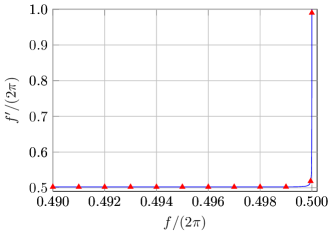
(a) $f^{\prime}(f)$.

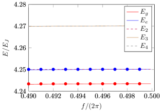
(b) $E(f)$.

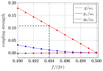
(c) $g(f)$.

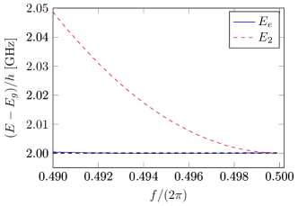
(d) Zoom in of LABEL:sub@fig:Ef.

Figure 2: (Color online). (a) The external flux $f^{\prime}$ as a function of $f$ for a fixed $\delta E$. (b) The five lowest eigenenergies of $\hat{H}_{\text{atom}}$ as a function of $f$ for a fixed $\delta E$. Results obtained via the numerical diagonalization are represented by lines with different colors. $E_{g}$ and $E_{e}$ obtained by Eqs. (23) and (24) are denoted as red and blue solid circles respectively. (c) The coupling strength as a function of $f$ for a fixed $\delta E$. The triangles represent results obtained via the numerical diagonalization, and the solid lines represent results obtained by Eqs. (28), (29a) and (29b). (d) The energies $E_{e}$ and $E_{2}$ of two lowest excited states relative to $E_{g}$. The black dashed line represents the value of the fixed atomic frequency $\delta E/h$. Here we take $\dfrac{E_{J}}{E_{c}}=150,~{}E_{J}/h=300\rm{GHz}$ and $\delta E/h=\dfrac{\omega_{c}}{2\pi}=2.00005254655\rm{GHz}$, $L_{0}=0.06192867473\rm{nH}$, $L_{r}=12.29291953901\rm{nH}$.

From Eqs. (27) and (28), we can get

$$\begin{split}&\dfrac{g^{2}E^{2}_{b}}{8\omega_{0}\omega_{c}\lambda^{4}E^{2}_{J}}=\Delta^{2}e^{-\lambda^{2}}\sin^{2}\dfrac{f^{\prime}}{2}\\ =&\dfrac{11E_{b}\Delta^{2}e^{-\lambda^{2}}}{11E_{b}+3\lambda^{2}E_{c}}-\dfrac{3E_{b}E_{c}(\delta E-E_{c})}{(11E_{b}+3\lambda^{2}E_{c})E^{2}_{J}}.\end{split}$$ (30)

In this article, we attempt to tune the coupling strength $g$ from zero to a finite value. In order to get an extremely small $g$, we should have $\delta E>E_{c}$ according to Eq. (30). In this sense, $f^{\prime}$ needs to satisfy the condition that

$$f^{\prime}>2\pi-\arccos\left(\dfrac{3\lambda^{4}-11}{11+3\lambda^{4}}\right)$$ (31)

for $\delta E$ being fixed.

As illustrated in Fig. 2a, we show how to change $f^{\prime}$ for different $f$ to keep the atomic energy level splitting $\delta E$ constant. With the same relation between $f^{\prime}$ and $f$, the five lowest eigenenergies of $\hat{H}_{\text{atom}}$ and the coupling strength $g$ as functions of $f$ are given in Figs. 2b and 2c respectively. When we zoom in Fig. 2b, we observe that $E_{e}-E_{g}$ is invariant with external flux $f$ which can seen in Fig. 2d.

In Fig. 2c, we observe that $g/\omega_{c}$ becomes smaller with the increase of $f$, and it limits to zero when $f$ tends to $\pi$. We also note that $|g_{0}/g|$ and $|g_{z}/g|$ increase with the decrease of $f$. When $f$ is far below $\pi$, $g_{z}$ is comparable with $g$ which makes it nonnegligible. In this case, our system can simulate a tunable coupling generalized Rabi model Braak (2011). If we restrict the value range of $f$ and $f^{\prime}$, we can get a tunable coupling Rabi model. For example, as shown in Fig. 2c, $|g_{z}/g|\ll 1$ and $|g_{0}/g|\ll 1$ when $f>0.988\pi$. Therefore, we can propose the tunable coupling scheme that changing the values of external flux $f$ and $f^{\prime}$ to tune the coupling strength from the extremely weak coupling regime to the ultrastrong coupling one and leave the energy splitting $\delta E$ unchanged. Moreover, it is worthy to point out that all the results in Fig. 2 obtained by quantum perturbation theory agree well with those from the numerical exact diagonalization, which verifies the validness of our calculations.

III Dissipation of the qubit

In general, the coupling of a superconducting qubit to its environment will cause two different dissipative processes, relaxation and pure dephasing, each with their characteristic time constants $T_{1}$ and $T_{\varphi}$. In this section, we discuss the performance of the qubit in terms of these two time constants in the tunable coupling scheme proposed above.

III.1 Estimates for the relaxation time $T_{1}$

As the de-excitation process of a qubit, the relaxation is originated from a perturbation which couples the qubit with its noise sources. In this perturbation, the qubit operator is defined as $\dfrac{\partial\hat{H}_{\rm{atom}}}{\partial\mu}$ where $\mu$ is the external parameter in the qubit’s Hamiltonian which corresponds to the noise source Ithier et al. (2005). For weak noise sources, we follow Ref. Schoelkopf et al. (2003) and give $T^{(\mu)}_{1}$ by Fermi’s golden rule

$$\Gamma^{(\mu)}_{1}=\dfrac{1}{T^{(\mu)}_{1}}=\dfrac{1}{\hbar^{2}}\left|\left\langle e\left|\dfrac{\partial\hat{H}_{\text{atom}}}{\partial\mu}\right|g\right\rangle\right|^{2}S_{\mu}(\omega),$$ (32)

where $S_{\mu}(\omega)$ is the spectral density of the bath noise. To this end, we can obtain the relaxation time with Eq. (32).

Compared to other solid-state qubits Bouchiat et al. (1998); Nakamura et al. (1999); Friedman et al. (2000); Der Wal et al. (2000); Koch et al. (2007); Barends et al. (2013), our qubit is remarkably sensitive to flux noise due to its unique structure. Therefore, it is reasonable to investigate the qubit’s dissipation caused by the flux noise at first.

Reviewing the qubit architecture in Fig. 1, we find that the coupling of our qubit to three external magnetic flux biases opens up an additional channel for energy relaxation, which is the internal coupling between the circuit and the flux biases through mutual inductance $M_{i}$ ($i=1,2,3$). After introducing the flux noise power spectrum

$$S_{\Phi_{i}}(\omega)=M^{2}_{i}S_{I_{i}}(\omega)=2M^{2}_{i}\Theta(\omega)\hbar\omega/Z_{\rm{R}}$$ (33)

with $\omega=\dfrac{\delta E}{\hbar}$ and the environmental impedance $Z_{\rm{R}}$ for low temperature $k_{B}T\ll\hbar\omega$, we get

$$\begin{split}T^{(\Phi)}_{1}\approx&\frac{\hbar^{2}\varphi^{2}_{0}Z_{\rm{R}}}{E^{2}_{J}\delta E}e^{\lambda^{2}}\left[M^{2}_{1}\cos^{2}\frac{\Delta+f^{\prime}}{2}+M^{2}_{2}\cos^{2}\frac{\Delta-f^{\prime}}{2}\right.\\ &\left.+\Delta^{2}M^{2}_{3}\sin^{2}\frac{f^{\prime}}{2}\right]^{-1}.\end{split}$$ (34)

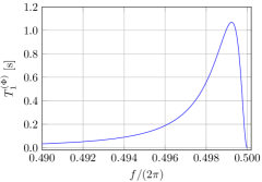
(a) $T^{(\Phi)}_{1}(f)$.

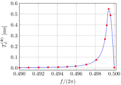
(b) $T^{(\Phi)}_{\varphi}(f)$.

Figure 3: (Color online). The characteristic time $T^{(\Phi)}_{1}$ and $T^{(\Phi)}_{\varphi}$ as a function of the external flux $f$. Here we take the same parameters as those of Fig. 2 and $M_{1}=M_{2}=40\Phi_{0}/A$, $M_{3}=35\Phi_{0}/A$, $Z_{\rm{R}}=50\Omega$, $A_{\Phi_{1}}=A_{\Phi_{2}}=A_{\Phi_{3}}=10^{-6}\Phi_{0}$. In Fig. LABEL:sub@fig:T2, the red triangles represent results obtained via the numerical diagonalization, and the solid lines represent results obtained by Eq. (37).

With the same qubit for Fig. 2 and realistic device parameters, we plot the relation between the relaxation time $T^{(\Phi)}_{1}$ and $f$. As shown in Fig. 3a, $T^{(\Phi)}_{1}$ reaches its maximum ($1.06893\rm{s}$) near $f=0.998487\pi$. Obviously, $T^{(\Phi)}_{1}$ is much longer than the time unit (ns) of a clock cycle used in experiments, which indicates that the relaxation induced by flux coupling is unlikely to limit the manipulation of our qubit.

Similar to the flux noise, the charge noise is an important noise source which limits the applications of charge type superconducting qubits. To our qubit, the charge noise corresponds to the qubit operator $\dfrac{\partial\hat{H}_{\rm{atom}}}{\partial\hat{n}_{-}}=2E_{c}\hat{n}_{-}$.

Since $\hat{n}_{-}\hat{P}+\hat{P}\hat{n}_{-}=0$, we have

$$\langle e|\hat{n}_{-}|g\rangle=\langle e|\hat{n}_{-}\hat{P}\hat{P}|g\rangle=-\langle e|\hat{P}\hat{n}_{-}\hat{P}|g\rangle=-\langle e|\hat{n}_{-}|g\rangle,$$ (35)

which implies that $\langle e|\hat{n}_{-}|g\rangle=0$. With Eqs. (32) and (35), we can show that the relaxation transition rate of our qubit induced by the charge noise is zero. In this sense, the charge noise will not affect the relaxation process of our qubit in the tunable coupling scheme.

III.2 Estimation of the pure dephasing time $T_{\varphi}$

The coupling with the environment results not only in relaxation but also in pure dephasing. As we know, the origin of dephasing can be interpreted as the qubit transition frequency fluctuations induced by noises from outside. In order to study the dephasing of our qubit, we define $T_{\varphi}$ as the characteristic time for the decay of the off-diagonal density matrix element. For sufficiently low frequencies, we assume that the environment provides $1/f$ noise Paladino et al. (2014) to our qubit. In this sense, we have Koch et al. (2007)

$$T^{(s)}_{\varphi}\simeq\dfrac{\hbar}{A_{s}}\left|\dfrac{\partial\delta E}{\partial s}\right|^{-1},$$ (36)

where $A_{s}$ is the $1/f$ amplitude corresponding to the external parameter represented by $s$ for different noise sources.

According to Eq. (27), $\delta E$ is dominated by the external flux and the Josephson energy $E_{J}$, which implies that the flux noise and the critical current noise are the main noise sources for our qubit. By Eq. (36), we have

$$\begin{split}T^{(\Phi)}_{\varphi}=&\dfrac{2\hbar\varphi_{0}}{\Delta A_{\Phi}E^{2}_{J}}e^{\lambda^{2}}\left[\left(\dfrac{11}{3E_{c}}-\dfrac{\lambda^{2}}{E_{b}}\right)+\left(\dfrac{11}{3E_{c}}+\dfrac{\lambda^{2}}{E_{b}}\right)\right.\\ &\times\left(\cos f^{\prime}-\dfrac{3\Delta}{2}\sin f^{\prime}\right)+\left|\left(\dfrac{11}{3E_{c}}-\dfrac{\lambda^{2}}{E_{b}}\right)\right.\\ &\left.\left.+\left(\dfrac{11}{3E_{c}}+\dfrac{\lambda^{2}}{E_{b}}\right)\left(\cos f^{\prime}+\dfrac{\Delta}{2}\sin f^{\prime}\right)\right|\right]^{-1}\end{split}$$ (37)

with $A_{\Phi}=A_{\Phi_{1}}=A_{\Phi_{2}}=A_{\Phi_{3}}$. For $A_{\Phi}=10^{-6}\Phi_{0}$ Yoshihara et al. (2006), the same qubit of Fig. 2 yields a dephasing time of the order of $T^{(\Phi)}_{\varphi}\sim 10\rm{\mu s}$. Fig. 3b shows the variation of $T^{(\Phi)}_{\varphi}$ with $f$ in our tunable coupling scheme.

For the critical current noise, we choose $A_{I_{c}}=10^{-6}I_{c}$ Van Harlingen et al. (2004). Then Eq. (36) gives

$$T^{(I_{c})}_{\varphi}\simeq\dfrac{\hbar}{A_{I_{c}}}\left|\dfrac{\partial\delta E}{\partial I_{c}}\right|^{-1}=\dfrac{\hbar}{2(A_{I_{c}}/I_{c})(\delta E-E_{c})}\approx 1.51442s$$ (38)

for our qubit in Fig. 2.

Furthermore, the fluctuation of our qubit transition frequency can also be induced by the fluctuation of the relative cooper pair number between the two dc-SQUIDs. Assuming that the relative cooper pair number $\hat{n}_{c}$ can be decomposed into the noiseless charge number $\hat{n}_{-}$ and a small noise term, i.e., $\hat{n}_{c}=\hat{n}_{-}+\delta n_{-}$ with $\delta n_{-}\ll n_{-}$. Then a Taylor expansion of $\hat{H}_{\rm{atom}}$ yields

$$\hat{H}_{\rm{atom}}\to\hat{H}_{0}+\hat{V}+2E_{c}\hat{n}_{-}\delta n_{-}.$$ (39)

Considering the relation between $\hat{n}_{-}$ and the parity operator $\hat{P}$, we introduce the odd-parity excited state $|\psi_{-}\rangle$ with its corresponding eigenenergy

$$E_{2}=\dfrac{E_{b}}{2}+E_{c}+4E_{J}-\Delta^{2}E^{2}_{J}e^{-\lambda^{2}}\left(\dfrac{\cos^{2}\dfrac{f^{\prime}}{2}}{3E_{c}}+\dfrac{\lambda^{2}\sin^{2}\dfrac{f^{\prime}}{2}}{E_{b}+3E_{c}}\right).$$ (40)

Therefore, we use

$$\langle\psi_{-}|\hat{n}_{-}|g\rangle \approx-\dfrac{i\sqrt{2}\Delta E_{J}e^{-\lambda^{2}/2}\cos\dfrac{f^{\prime}}{2}}{E_{c}},$$ (41a)

$$\langle\psi_{-}|\hat{n}_{-}|e\rangle \approx 1+2\Delta^{2}E^{2}_{J}e^{-\lambda^{2}}\left(\dfrac{\cos^{2}\dfrac{f^{\prime}}{2}}{9E^{2}_{c}}-\dfrac{\lambda^{2}\sin^{2}\dfrac{f^{\prime}}{2}}{(E_{b}+3E_{c})^{2}}\right)$$ (41b)

to get the modification of the energy level splitting $\delta E(n_{-})$ from the coupling between $|\psi_{-}\rangle$ and $|e\rangle$, $|g\rangle$ by the charge noise term $2E_{c}\hat{n}_{-}\delta n_{-}$

$$\begin{split}\delta[\delta E]=&\delta E(n_{-}+\delta n_{-})-\delta E(n_{-})\\ =&4E^{2}_{c}(\delta n_{-})^{2}\left(\dfrac{|\langle\psi_{-}|\hat{n}_{-}|g\rangle|^{2}}{E_{2}-E_{g}}-\dfrac{|\langle\psi_{-}|\hat{n}_{-}|e\rangle|^{2}}{E_{2}-E_{e}}\right),\end{split}$$ (42)

which is proportional to the square of $\delta n_{-}$. In other words, the second order contributions of the charge noise will dominate the pure dephasing process.

(a) $T^{(c)}_{\varphi}(f)$.

(b) Zoom in of LABEL:sub@fig:T2CN.

Figure 4: (Color online). The characteristic time $T^{(c)}_{\varphi}$ as a function of the external flux $f$. Here we take the same parameters as those of Fig. 2 and $A_{c}=10^{-4}e$.

Based on the above consideration, we generalize Eq. (36) to the second order

$$\begin{split}T^{(c)}_{\varphi}\simeq&\left|\dfrac{\pi^{2}A^{2}_{c}}{\hbar}\dfrac{\partial^{2}\delta E}{\partial(e\delta n_{-})^{2}}\right|^{-1}\\ =&\dfrac{\hbar e^{2}}{\pi^{2}A^{2}_{c}}\left|\lim_{\delta n_{-}\to 0}\left[\dfrac{\delta E(n_{-}+2\delta n_{-})-\delta E(n_{-}+\delta n_{-})}{(\delta n_{-})^{2}}\right.\right.\\ &\quad\qquad\left.\left.-\dfrac{\delta E(n_{-}+\delta n_{-})-\delta E(n_{-})}{(\delta n_{-})^{2}}\right]\right|^{-1}\\ =&\dfrac{\hbar e^{2}}{8\pi^{2}A^{2}_{c}E^{2}_{c}}\left|\dfrac{|\langle\psi_{-}|\hat{n}_{-}|g\rangle|^{2}}{E_{2}-E_{g}}-\dfrac{|\langle\psi_{-}|\hat{n}_{-}|e\rangle|^{2}}{E_{2}-E_{e}}\right|^{-1},\end{split}$$ (43)

where $A_{c}$ is the amplitude of the charge $1/f$ noise.

With the same parameters in Fig. 2 and $A_{c}=10^{-4}e$ Zorin et al. (1996), we find that $T^{(c)}_{\varphi}$ reaches its minimum $1.00293\rm{ms}$ near $f=0.99951\pi$ which can be seen in Fig. 4. In this sense, our qubit has an excellent performance suppressing the charge noise.

IV Estimation of device parameters

In order to apply our design to experiments, we should choose proper value of device parameters such as $L_{0}$, $L_{r}$. In this paper, we attempt to tune the atom-photon coupling strength from weak coupling regime into the ultra strong one while keeping the cavity frequency and the atomic frequency invariant. With Eq. (28), we can write the formula of the coupling strength with respect to the cavity frequency

$$\dfrac{g}{\omega_{c}}=\sqrt{\dfrac{8\omega_{0}}{\omega_{c}}}\Delta\lambda^{4}\dfrac{E_{J}}{E_{c}}e^{-\lambda^{2}/2}\sin\dfrac{f^{\prime}}{2},$$ (44)

which indicates that $\lambda$, the ratio $\dfrac{E_{J}}{E_{c}}$ and $\dfrac{\omega_{0}}{\omega_{c}}$ are the main factors influencing its value.

During the derivation process of $\delta E$ and $g$, we assume that $\Delta\ll\pi$ and $\lambda\ll 1$ ($E_{b}\gg E_{c}$) to ensure the establishment of quantum perturbation theory. In this sense, we have

$$\dfrac{1}{2L_{0}}+\dfrac{1}{L_{r}}=\dfrac{1}{L^{\prime}_{r}}\gg\dfrac{E_{c}}{8\varphi^{2}_{0}},$$ (45)

which means that $L_{0}$ and $L_{r}$ are both far more less than $\dfrac{8\varphi^{2}_{0}}{E_{c}}$. In Fig. 2, we take $E_{c}/h=2\rm{GHz}$, then Eq. (45) gives $\{L_{0},L_{r}\}\ll 0.653983\rm{\mu H}$ which implies the reasonableness of our choice.

Generally, the relaxation time of a qubit in a circuit QED experiment should be long enough. According to Eqs. (34), (37), (38) and (43), the characteristic time $T_{1}$ and $T_{\varphi}$ are proportional to the ratio $\dfrac{E_{J}}{E_{c}}$ once $E_{J}$ is fixed. It seems that we need to take $\dfrac{E_{J}}{E_{c}}\gg 1$ to get a sufficiently large coupling strength. However, as expressed in Eqs. (29a) and (29b), the ratio $\dfrac{g_{z}}{g}$ and $\dfrac{g_{0}}{g}$ are inversely proportional to $\dfrac{E_{J}}{E_{c}}$. Therefore the value of $\dfrac{E_{J}}{E_{c}}$ should be restricted by $\left|\dfrac{g_{z}}{g}\right|\ll 1$ if we want to simulate the Rabi model.

Besides, focusing on Eq. (44), we can find that the transverse coupling strength is proportional to the square root of $\dfrac{\omega_{0}}{\omega_{c}}$. This indicates that we need to take a sufficiently small $L_{0}$ to obtain a relatively large $\dfrac{g}{\omega_{c}}$.

V Conclusion

In this article, we present a theoretical proposal with a tunable coupling between an artificial two-level atom and a waveguide transmission line resonator by controlling the external magnetic fluxes. In our scheme, the coupling can be continuously tuned from zero to the ultrastrong regime while keeping fixed atomic level splitting. We also investigate the performance of our qubit under the influences of the environment, and find that our system operates well against the main noises. Our analytical results are based on quantum perturbation theory with the parity symmetry, which are verified by the numerical simulations. In order to apply our qubit design to experiments, we discuss how to choose the device parameters by our analytical results. We hope that our work will stimulate the coherent manipulation of the circuit QED system in the fields of quantum simulation and quantum computing.

Appendix A Derivation of the energy splitting and the coupling strength

Because $E_{b}\gg E_{c}$, we can restrict ourselves in the subspace with the bases $\{|n=0\rangle,|n=1\rangle\}$. In this subspace, the term

$$\begin{split}&\cos(\phi_{+}+\frac{f^{\prime}}{2})=\cos\frac{f^{\prime}}{2}\cos\phi_{+}-\sin\frac{f^{\prime}}{2}\sin\phi_{+}\\ =&\cos\frac{f^{\prime}}{2}\left(\langle 0|\cos\phi_{+}|0\rangle|0\rangle\langle 0|+\langle 1|\cos\phi_{+}|1\rangle|1\rangle\langle 1|\right)-\sin\frac{f^{\prime}}{2}\left(\langle 0|\sin\phi_{+}|1\rangle|0\rangle\langle 1|+\langle 1|\sin\phi_{+}|0\rangle|1\rangle\langle 0|\right)\\ =&\cos\frac{f^{\prime}}{2}\left(e^{-\lambda^{2}/2}|0\rangle\langle 0|+(1-\lambda^{2})e^{-\lambda^{2}/2}|1\rangle\langle 1|\right)-\sin\frac{f^{\prime}}{2}\lambda e^{-\lambda^{2}/2}\left(|0\rangle\langle 1|+|1\rangle\langle 0|\right),\end{split}$$ (46)

where we use the following expressions:

$$\langle 0|\cos\phi_{+}|0\rangle=\frac{1}{2}\left(\langle 0|e^{i\lambda(\hat{b}+\hat{b}^{\dagger})}|0\rangle+\langle 0|e^{-i\lambda(\hat{b}+\hat{b}^{\dagger})}|0\rangle\right)=\frac{e^{-\lambda^{2}/2}}{2}\left(\langle 0|e^{i\lambda\hat{b}^{\dagger}}e^{i\lambda\hat{b}}|0\rangle+\langle 0|e^{-i\lambda\hat{b}^{\dagger}}e^{-i\lambda\hat{b}}|0\rangle\right)=e^{-\lambda^{2}/2},$$ (47)

$$\langle 1|\cos\phi_{+}|1\rangle=\frac{1}{2}\left(\langle 1|e^{i\lambda(\hat{b}+\hat{b}^{\dagger})}|1\rangle+\langle 1|e^{-i\lambda(\hat{b}+\hat{b}^{\dagger})}|1\rangle\right)=\frac{e^{-\lambda^{2}/2}}{2}\left(\langle 1|e^{i\lambda\hat{b}^{\dagger}}e^{i\lambda\hat{b}}|1\rangle+\langle 1|e^{-i\lambda\hat{b}^{\dagger}}e^{-i\lambda\hat{b}}|1\rangle\right)=(1-\lambda^{2})e^{-\lambda^{2}/2},$$ (48)

$$\langle 1|\sin\phi_{+}|0\rangle=\frac{1}{2i}\left(\langle 1|e^{i\lambda(\hat{b}+\hat{b}^{\dagger})}|0\rangle-\langle 1|e^{-i\lambda(\hat{b}+\hat{b}^{\dagger})}|0\rangle\right)=\frac{e^{-\lambda^{2}/2}}{2i}\left(\langle 1|e^{i\lambda\hat{b}^{\dagger}}e^{i\lambda\hat{b}}|0\rangle-\langle 1|e^{-i\lambda\hat{b}^{\dagger}}e^{-i\lambda\hat{b}}|0\rangle\right)=\lambda e^{-\lambda^{2}/2},$$ (49)

$$\langle 0|\sin\phi_{+}|1\rangle=(\langle 1|\sin\phi_{+}|0\rangle)^{\ast}=\lambda e^{-\lambda^{2}/2}.$$ (50)

In addition, in the subspace with even parity $\{|0\rangle,|+\rangle_{n}\}$, the term

$$-2\sin\left(\phi_{-}+\frac{\Delta}{2}\right)=i\left(e^{i\left(\phi_{-}+\frac{\Delta}{2}\right)}-e^{-i\left(\phi_{-}+\frac{\Delta}{2}\right)}\right)=i\sum_{n>0}\left(|+_{n+1}\rangle\langle+_{n}|-|+_{n}\rangle\langle+_{n+1}|\right)+i\sqrt{2}(|+_{1}\rangle\langle 0|-|0\rangle\langle+_{1}|).$$ (51)

Thus we obtain the expression for the perturbation $\hat{V}$ in the relative subspace for our problem. Using the perturbation theory, we obtain

$$\begin{split}|g\rangle=&|0;0\rangle-\dfrac{\langle 0;+_{1}|\hat{V}|0;0\rangle}{E_{c}}|0;+_{1}\rangle-\dfrac{\langle 1;+_{1}|\hat{V}|0;0\rangle}{E_{b}+E_{c}}|1;+_{1}\rangle+\dfrac{\langle 0;+_{2}|\hat{V}|0;+_{1}\rangle\langle 0;+_{1}|\hat{V}|0;0\rangle}{4E^{2}_{c}}|0;+_{2}\rangle\\ &+\dfrac{\langle 0;+_{2}|\hat{V}|1;+_{1}\rangle\langle 1;+_{1}|\hat{V}|0;0\rangle}{4E_{c}(E_{b}+E_{c})}|0;+_{2}\rangle+\dfrac{\langle 1;+_{2}|\hat{V}|0;+_{1}\rangle\langle 0;+_{1}|\hat{V}|0;0\rangle}{(E_{b}+4E_{c})E_{c}}|1;+_{2}\rangle\\ &+\dfrac{\langle 1;+_{2}|\hat{V}|1;+_{1}\rangle\langle 1;+_{1}|\hat{V}|0;0\rangle}{(E_{b}+4E_{c})(E_{b}+E_{c})}|1;+_{2}\rangle+\dfrac{\langle 1;0|\hat{V}|0;+_{1}\rangle\langle 0;+_{1}|\hat{V}|0;0\rangle}{E_{b}E_{c}}|1;0\rangle\\ &+\dfrac{\langle 1;0|\hat{V}|1;+_{1}\rangle\langle 1;+_{1}|\hat{V}|0;0\rangle}{E_{b}(E_{b}+E_{c})}|1;0\rangle,\\ \end{split}$$ (52)

and

$$\begin{split}|e\rangle=&|0;+_{1}\rangle-\dfrac{\langle 0;+_{2}|\hat{V}|0;+_{1}\rangle}{3E_{c}}|0;+_{2}\rangle+\dfrac{\langle 0;0|\hat{V}|0;+_{1}\rangle}{E_{c}}|0;0\rangle-\dfrac{\langle 1;+_{2}|\hat{V}|0;+_{1}\rangle}{E_{b}+3E_{c}}|1;+_{2}\rangle-\dfrac{\langle 1;0|\hat{V}|0;+_{1}\rangle}{E_{b}-E_{c}}|1;0\rangle\\ &+\dfrac{\langle 0;+_{3}|\hat{V}|0;+_{2}\rangle\langle 0;+_{2}|\hat{V}|0;+_{1}\rangle}{24E^{2}_{c}}|0;+_{3}\rangle+\dfrac{\langle 0;+_{3}|\hat{V}|1;+_{2}\rangle\langle 1;+_{2}|\hat{V}|0;+_{1}\rangle}{8E_{c}(E_{b}+3E_{c})}|0;+_{3}\rangle\\ &+\dfrac{\langle 1;+_{3}|\hat{V}|0;+_{2}\rangle\langle 0;+_{2}|\hat{V}|0;+_{1}\rangle}{3E_{c}(E_{b}+8E_{c})}|1;+_{3}\rangle+\dfrac{\langle 1;+_{3}|\hat{V}|1;+_{2}\rangle\langle 1;+_{2}|\hat{V}|0;+_{1}\rangle}{(E_{b}+8E_{c})(E_{b}+3E_{c})}|1;+_{3}\rangle\\ &+\dfrac{\langle 1;+_{1}|\hat{V}|0;+_{2}\rangle\langle 0;+_{2}|\hat{V}|0;+_{1}\rangle}{3E_{b}E_{c}}|1;+_{1}\rangle-\dfrac{\langle 1;+_{1}|\hat{V}|0;0\rangle\langle 0;0|\hat{V}|0;+_{1}\rangle}{E_{b}E_{c}}|1;+_{1}\rangle\\ &+\dfrac{\langle 1;+_{1}|\hat{V}|1;+_{2}\rangle\langle 1;+_{2}|\hat{V}|0;+_{1}\rangle}{E_{b}(E_{b}+3E_{c})}|1;+_{1}\rangle+\dfrac{\langle 1;+_{1}|\hat{V}|1;0\rangle\langle 1;0|\hat{V}|0;+_{1}\rangle}{E_{b}(E_{b}-E_{c})}|1;+_{1}\rangle,\end{split}$$ (53)

where

$$\langle 0;+_{1}|\hat{V}|0;0\rangle=i\sqrt{2}\Delta E_{J}e^{-\lambda^{2}/2}\cos\dfrac{f^{\prime}}{2},$$ (54a)

$$\langle 1;+_{1}|\hat{V}|0;0\rangle=\langle 0;+_{1}|\hat{V}|1;0\rangle=-i\sqrt{2}\Delta E_{J}\lambda e^{-\lambda^{2}/2}\sin\dfrac{f^{\prime}}{2},$$ (54b)

$$\langle 0;+_{2}|\hat{V}|0;+_{1}\rangle=\langle 0;+_{3}|\hat{V}|0;+_{2}\rangle=i\Delta E_{J}e^{-\lambda^{2}/2}\cos\dfrac{f^{\prime}}{2},$$ (54c)

$$\langle 1;+_{2}|\hat{V}|0;+_{1}\rangle=\langle 0;+_{2}|\hat{V}|1;+_{1}\rangle=\langle 0;+_{3}|\hat{V}|1;+_{2}\rangle=\langle 1;+_{3}|\hat{V}|0;+_{2}\rangle=-i\Delta E_{J}\lambda e^{-\lambda^{2}/2}\sin\dfrac{f^{\prime}}{2},$$ (54d)

$$\langle 1;+_{2}|\hat{V}|1;+_{1}\rangle=\langle 1;+_{3}|\hat{V}|1;+_{2}\rangle=i\Delta E_{J}(1-\lambda^{2})e^{-\lambda^{2}/2}\cos\dfrac{f^{\prime}}{2},$$ (54e)

$$\langle 1;0|\hat{V}|1;+_{1}\rangle=-i\sqrt{2}\Delta E_{J}(1-\lambda^{2})e^{-\lambda^{2}/2}\cos\dfrac{f^{\prime}}{2}.$$ (54f)

Therefore

$$\begin{split}E_{g}=&\frac{1}{2}E_{b}+4E_{J}-2\Delta^{2}\frac{E_{J}^{2}}{E_{c}}\cos^{2}\frac{f^{\prime}}{2}e^{-\lambda^{2}}-2\Delta^{2}\frac{E_{J}^{2}}{E_{b}+E_{c}}\sin^{2}\frac{f^{\prime}}{2}\lambda^{2}e^{-\lambda^{2}}\\ \approx&\frac{1}{2}E_{b}+4E_{J}-2\Delta^{2}E_{J}^{2}e^{-\lambda^{2}}\left(\dfrac{\cos^{2}\dfrac{f^{\prime}}{2}}{E_{c}}+\dfrac{\lambda^{2}\sin^{2}\dfrac{f^{\prime}}{2}}{E_{b}}\right),\end{split}$$ (55)

$$\begin{split}E_{e}=&\frac{1}{2}E_{b}+E_{c}+4E_{J}+\frac{5}{3}\Delta^{2}\frac{E_{J}^{2}}{E_{c}}\cos^{2}\frac{f^{\prime}}{2}e^{-\lambda^{2}}-2\Delta^{2}\frac{E_{J}^{2}}{E_{b}-E_{c}}\sin^{2}\frac{f^{\prime}}{2}\lambda^{2}e^{-\lambda^{2}}-\Delta^{2}\frac{E_{J}^{2}}{E_{b}+3E_{c}}\sin^{2}\frac{f^{\prime}}{2}\lambda^{2}e^{-\lambda^{2}}\\ \approx&\frac{1}{2}E_{b}+E_{c}+4E_{J}+\Delta^{2}E_{J}^{2}e^{-\lambda^{2}}\left(\dfrac{5\cos^{2}\dfrac{f^{\prime}}{2}}{3E_{c}}-\dfrac{3\lambda^{2}\sin^{2}\dfrac{f^{\prime}}{2}}{E_{b}}\right).\end{split}$$ (56)

Then the energy splitting is

$$\begin{split}\delta E=&E_{e}-E_{g}=E_{c}+\frac{11}{3}\Delta^{2}\frac{E_{J}^{2}}{E_{c}}\cos^{2}\frac{f^{\prime}}{2}e^{-\lambda^{2}}-4\Delta^{2}\frac{E_{c}E_{J}^{2}}{E_{b}^{2}-E_{c}^{2}}\sin^{2}\frac{f^{\prime}}{2}\lambda^{2}e^{-\lambda^{2}}-\Delta^{2}\frac{E_{J}^{2}}{E_{b}+3E_{c}}\sin^{2}\frac{f^{\prime}}{2}\lambda^{2}e^{-\lambda^{2}}\\ \approx&E_{c}+\Delta^{2}E_{J}^{2}e^{-\lambda^{2}}\left(\frac{11}{3E_{c}}\cos^{2}\frac{f^{\prime}}{2}-\dfrac{\lambda^{2}}{E_{b}}\sin^{2}\dfrac{f^{\prime}}{2}\right).\end{split}$$ (57)

The approximation is valid due to the assumption $E_{b}\gg E_{c}$.

Now we can calculate the operator $\hat{\phi}_{+}$ up to the second order:

$$\begin{split}\langle g|\hat{\phi}_{+}|g\rangle\approx&\lambda\left(\dfrac{\langle 0;0|\hat{V}|0;+_{1}\rangle\langle 1;+_{1}|\hat{V}|0;0\rangle}{E_{c}(E_{b}+E_{c})}+\dfrac{\langle 1;0|\hat{V}|0;+_{1}\rangle\langle 0;+_{1}|\hat{V}|0;0\rangle}{E_{b}E_{c}}+\dfrac{\langle 1;0|\hat{V}|1;+_{1}\rangle\langle 1;+_{1}|\hat{V}|0;0\rangle}{E_{b}(E_{b}+E_{c})}+\text{h.c.}\right)\\ =&-2\Delta^{2}E^{2}_{J}\lambda^{2}e^{-\lambda^{2}}\sin f^{\prime}\left[\dfrac{1}{E_{c}(E_{b}+E_{c})}+\dfrac{1}{E_{b}E_{c}}+\dfrac{1-\lambda^{2}}{E_{b}(E_{b}+E_{c})}\right]\\ =&-2\Delta^{2}E^{2}_{J}\lambda^{2}\dfrac{2E_{b}+(2-\lambda^{2})E_{c}}{E_{b}E_{c}(E_{b}+E_{c})}e^{-\lambda^{2}}\sin f^{\prime}\approx-\dfrac{4\Delta^{2}E^{2}_{J}\lambda^{2}e^{-\lambda^{2}}\sin f^{\prime}}{E_{b}E_{c}},\\ \end{split}$$ (58)

$$\begin{split}\langle e|\hat{\phi}_{+}|e\rangle\approx&\lambda\left(\dfrac{\langle 1;+_{2}|\hat{V}|0;+_{1}\rangle\langle 0;+_{1}|\hat{V}|0;+_{2}\rangle}{3E_{c}(E_{b}+3E_{c})}-\dfrac{\langle 1;0|\hat{V}|0;+_{1}\rangle\langle 0;+_{1}|\hat{V}|0;0\rangle}{E_{c}(E_{b}-E_{c})}+\dfrac{\langle 1;+_{1}|\hat{V}|0;+_{2}\rangle\langle 0;+_{2}|\hat{V}|0;+_{1}\rangle}{3E_{b}E_{c}}\right.\\ &\left.-\dfrac{\langle 1;+_{1}|\hat{V}|0;0\rangle\langle 0;0|\hat{V}|0;+_{1}\rangle}{E_{b}E_{c}}+\dfrac{\langle 1;+_{1}|\hat{V}|1;+_{2}\rangle\langle 1;+_{2}|\hat{V}|0;+_{1}\rangle}{E_{b}(E_{b}+3E_{c})}+\dfrac{\langle 1;+_{1}|\hat{V}|1;0\rangle\langle 1;0|\hat{V}|0;+_{1}\rangle}{E_{b}(E_{b}-E_{c})}+\text{h.c.}\right)\\ =&2\Delta^{2}E^{2}_{J}\lambda^{2}e^{-\lambda^{2}}\left[\sin f^{\prime}\left(\dfrac{5}{6E_{b}E_{c}}+\dfrac{1}{E_{c}(E_{b}-E_{c})}-\dfrac{3(1-\lambda^{2})E_{c}+E_{b}}{6E_{b}E_{c}(E_{b}+3E_{c})}\right)-\dfrac{\lambda(1-\cos f^{\prime})}{E_{b}(E_{b}-E_{c})}\right]\\ =&2\Delta^{2}E^{2}_{J}\lambda^{2}e^{-\lambda^{2}}\left[\dfrac{\lambda(\cos f^{\prime}-1)}{E_{b}(E_{b}-E_{c})}+\dfrac{10E^{2}_{b}+(26+3\lambda^{2})E_{b}E_{c}-3(4+\lambda^{2})E^{2}_{c}}{6E_{b}E_{c}(E_{b}+3E_{c})(E_{b}-E_{c})}\sin f^{\prime}\right]\\ \approx&\dfrac{10}{3}\Delta^{2}\dfrac{E^{2}_{J}}{E_{b}E_{c}}\lambda^{2}e^{-\lambda^{2}}\sin f^{\prime},\end{split}$$ (59)

and

$$\langle e|\hat{\phi}_{+}|g\rangle\approx-\dfrac{\lambda\langle 1;+_{1}|\hat{V}|0;0\rangle}{E_{b}+E_{c}}-\dfrac{\lambda(\langle 1;0|\hat{V}|0;+_{1}\rangle)^{\ast}}{E_{b}-E_{c}}=\dfrac{i2\sqrt{2}\Delta E_{J}E_{b}\lambda^{2}e^{-\lambda^{2}/2}}{E^{2}_{b}-E^{2}_{c}}\sin\dfrac{f^{\prime}}{2}\approx\dfrac{i2\sqrt{2}\Delta E_{J}\lambda^{2}e^{-\lambda^{2}/2}}{E_{b}}\sin\dfrac{f^{\prime}}{2}.$$ (60)

With Eqs. (58), (59) and (60), we can rewrite Eq. (22b) as

$$\hat{H}_{\text{int}}=\hbar(g_{x}\hat{\sigma}_{x}+g\hat{\sigma}_{y}+g_{0}\hat{\sigma}_{0}+g_{z}\hat{\sigma}_{z})(\hat{a}^{\dagger}+\hat{a}),$$ (61)

where

$$g_{x}= -\sqrt{\omega_{0}\omega_{c}}\dfrac{\langle e|\hat{\phi}_{+}|g\rangle+\langle g|\hat{\phi}_{+}|e\rangle}{2}=0,$$ (62a)

$$g= -i\sqrt{\omega_{0}\omega_{c}}\dfrac{\langle e|\hat{\phi}_{+}|g\rangle-\langle g|\hat{\sigma}_{+}|e\rangle}{2}\approx\dfrac{\sqrt{8\omega_{0}\omega_{c}}\Delta E_{J}\lambda^{2}e^{-\lambda^{2}/2}}{E_{b}}\sin\dfrac{f^{\prime}}{2},$$ (62b)

$$g_{0}= -\sqrt{\omega_{0}\omega_{c}}\dfrac{\langle e|\hat{\phi}_{+}|e\rangle+\langle g|\hat{\phi}_{+}|g\rangle}{2}\approx\dfrac{\sqrt{\omega_{0}\omega_{c}}\Delta^{2}E^{2}_{J}\lambda^{2}e^{-\lambda^{2}}}{3E_{b}E_{c}}\sin f^{\prime},$$ (62c)

$$g_{z}= -\sqrt{\omega_{0}\omega_{c}}\dfrac{\langle e|\hat{\phi}_{+}|e\rangle-\langle g|\hat{\phi}_{+}|g\rangle}{2}\approx-\dfrac{11\sqrt{\omega_{0}\omega_{c}}\Delta^{2}E^{2}_{J}\lambda^{2}e^{-\lambda^{2}}}{3E_{b}E_{c}}\sin f^{\prime}.$$ (62d)

References

- Toyli et al. (2016) D. M. Toyli, A. W. Eddins, S. Boutin, S. Puri, D. Hover, V. Bolkhovsky, W. D. Oliver, A. Blais, and I. Siddiqi, Phys. Rev. X 6, 031004 (2016).
- Borja Peropadre and Aspuru-Guzik (2016) J. H. Borja Peropadre, Gian Giacomo Guerreschi and A. Aspuru-Guzik, Phys. Rev. Lett. 117, 140505 (2016).
- Zhou et al. (2008) L. Zhou, Z. R. Gong, Y.-x. Liu, C. P. Sun, and F. Nori, Phys. Rev. Lett. 101, 100501 (2008).
- He et al. (2017) Q.-K. He, W. Zhu, Z. H. Wang, and D. L. Zhou, J. Phys. B: At. Mol. Opt. Phys. 50, 145002 (2017).
- Forn-Díaz et al. (2017) P. Forn-Díaz, J. García-Ripoll, B. Peropadre, J.-L. Orgiazzi, M. Yurtalan, R. Belyansky, C. Wilson, and A. Lupascu, Nat. Phys. 13, 39 (2017).
- Forndiaz et al. (2010) P. Forndiaz, J. Lisenfeld, D. Marcos, J. J. Garciaripoll, E. Solano, C. J. P. M. Harmans, and J. E. Mooij, Phys. Rev. Lett. 105, 237001 (2010).
- Gu et al. (2017) X. Gu, A. F. Kockum, A. Miranowicz, Y. xi Liu, and F. Nori, Physics Reports 718-719, 1 (2017).
- Yoshihara et al. (2017) F. Yoshihara, T. Fuse, S. Ashhab, K. Kakuyanagi, S. Saito, and K. Semba, Nat. Phys. 13, 44 (2017).
- Peropadre et al. (2013a) B. Peropadre, D. Zueco, F. Wulschner, F. Deppe, A. Marx, R. Gross, and J. J. Garciaripoll, Phys. Rev. B 87 (2013a).
- Baust et al. (2015) A. Baust, E. Hoffmann, M. Haeberlein, M. J. Schwarz, P. Eder, E. P. Menzel, K. G. Fedorov, J. Goetz, F. Wulschner, E. Xie, et al., Phys. Rev. B 91 (2015).
- Wulschner et al. (2016) F. Wulschner, J. Goetz, F. R. Koessel, E. Hoffmann, A. Baust, P. Eder, M. Fischer, M. Haeberlein, M. J. Schwarz, M. Pernpeintner, et al., EPJ Quantum Technology 3, 10 (2016).
- Kim (2006) M. D. Kim, Phys. Rev. B 74, 184501 (2006).
- Tong et al. (2007) D. Tong, K. Singh, L. C. Kwek, and C. H. Oh, Phys. Rev. Lett. 98, 150402 (2007).
- Martinis et al. (2005) J. M. Martinis, K. B. Cooper, R. McDermott, M. Steffen, M. Ansmann, K. D. Osborn, K. Cicak, S. Oh, D. P. Pappas, R. W. Simmonds, and C. C. Yu, Phys. Rev. Lett. 95, 210503 (2005).
- Koch et al. (2007) J. Koch, M. Y. Terri, J. Gambetta, A. A. Houck, D. Schuster, J. Majer, A. Blais, M. H. Devoret, S. M. Girvin, and R. J. Schoelkopf, Phys. Rev. A 76, 042319 (2007).
- Barends et al. (2013) R. Barends, J. Kelly, A. Megrant, D. Sank, E. Jeffrey, Y. Chen, Y. Yin, B. Chiaro, J. Mutus, C. Neill, et al., Phys. Rev. Lett. 111, 080502 (2013).
- Inomata et al. (2012) K. Inomata, T. Yamamoto, P.-M. Billangeon, Y. Nakamura, and J. S. Tsai, Phys. Rev. B 86, 140508 (2012).
- Mariantoni et al. (2008) M. Mariantoni, F. Deppe, A. Marx, R. Gross, F. K. Wilhelm, and E. Solano, Phys. Rev. B 78, 104508 (2008).
- van den Brink et al. (2005) A. M. van den Brink, A. J. Berkley, and M. Yalowsky, New J. Phys. 7, 230 (2005).
- Peropadre et al. (2010) B. Peropadre, P. Forn-Díaz, E. Solano, and J. J. García-Ripoll, Phys. Rev. Lett. 105, 023601 (2010).
- Gambetta et al. (2011) J. M. Gambetta, A. A. Houck, and A. Blais, Phys. Rev. Lett. 106, 030502 (2011).
- Srinivasan et al. (2011) S. Srinivasan, A. Hoffman, J. Gambetta, and A. Houck, Phys. Rev. Lett. 106, 083601 (2011).
- Bruschi et al. (2013) D. E. Bruschi, A. R. Lee, and I. Fuentes, J. Phys. A: Math. Theor. 46, 165303 (2013).
- Mezzacapo et al. (2014) A. Mezzacapo, L. Lamata, S. Filipp, and E. Solano, Phys. Rev. Lett. 113, 050501 (2014).
- Lu et al. (2017) Y. Lu, S. Chakram, N. Leung, N. Earnest, R. K. Naik, Z. Huang, P. Groszkowski, E. Kapit, J. Koch, and D. I. Schuster, Phys. Rev. Lett. 119, 150502 (2017).
- Kyaw et al. (2015) T. H. Kyaw, S. Felicetti, G. Romero, E. Solano, and L. C. Kwek, Scientific Reports 5, 8621 (2015).
- Felicetti et al. (2015) S. Felicetti, C. Sabín, I. Fuentes, L. Lamata, G. Romero, and E. Solano, Phys. Rev. B 92, 064501 (2015).
- Garciaalvarez et al. (2017) L. Garciaalvarez, S. Felicetti, E. Rico, E. Solano, and C. Sabin, Scientific Reports 7, 657 (2017).
- Devoret (1995) M. Devoret, Les Houches, Session LXIII 7, 351 (1995).
- Peropadre et al. (2013b) B. Peropadre, D. Zueco, D. Porras, and J. J. García-Ripoll, Phys. Rev. Lett. 111, 243602 (2013b).
- Sakurai and Napolitano (2011) J. J. Sakurai and J. J. Napolitano, Modern Quantum Mechanics, 2nd Edition (Addison-Wesley & Pearson, 2011) pp. 285–304.
- Braak (2011) D. Braak, Phys. Rev. Lett. 107, 100401 (2011).
- Ithier et al. (2005) G. Ithier, E. Collin, P. Joyez, P. Meeson, D. Vion, D. Esteve, F. Chiarello, A. Shnirman, Y. Makhlin, J. Schriefl, et al., Phys. Rev. B 72, 134519 (2005).
- Schoelkopf et al. (2003) R. J. Schoelkopf, A. Clerk, S. Girvin, K. W. Lehnert, and M. Devoret, in Proc. SPIE, Vol. 5115 (International Society for Optics and Photonics, 2003) pp. 356–377.
- Bouchiat et al. (1998) V. Bouchiat, D. Vion, P. Joyez, D. Esteve, and M. Devoret, Physica Scripta 1998, 165 (1998).
- Nakamura et al. (1999) Y. Nakamura, Y. A. Pashkin, and J. S. Tsai, Nature 398, 786 (1999).
- Friedman et al. (2000) J. R. Friedman, V. Patel, W. Chen, S. K. Tolpygo, and J. E. Lukens, Nature (London) 406, 43 (2000).
- Der Wal et al. (2000) C. H. V. Der Wal, A. C. J. T. Haar, F. K. Wilhelm, R. N. Schouten, C. J. P. M. Harmans, T. P. Orlando, S. Lloyd, and J. E. Mooij, Science 290, 773 (2000).
- Paladino et al. (2014) E. Paladino, Y. Galperin, G. Falci, and B. Altshuler, Rev. Mod. Phys. 86, 361 (2014).
- Yoshihara et al. (2006) F. Yoshihara, K. Harrabi, A. Niskanen, Y. Nakamura, and J. Tsai, Phys. Rev. Lett. 97, 167001 (2006).
- Van Harlingen et al. (2004) D. Van Harlingen, T. Robertson, B. Plourde, P. Reichardt, T. Crane, and J. Clarke, Phys. Rev. B 70, 064517 (2004).
- Zorin et al. (1996) A. B. Zorin, F.-J. Ahlers, J. Niemeyer, T. Weimann, H. Wolf, V. A. Krupenin, and S. V. Lotkhov, Phys. Rev. B 53, 13682 (1996).