Abstract

We consider tomography of the Earth’s interior using the neutrino pair beam which has recently been proposed. The beam produces a large amount of neutrino and antineutrino pairs from the circulating partially stripped ions and provides the possibility to measure precisely the energy spectrum of neutrino oscillation probability together with a sufficiently large detector. It is shown that the pair beam gives a better sensitivity to probe the Earth’s crust compared with the neutrino sources at present. In addition we present a method to reconstruct a matter density profile by means of the analytic formula of the oscillation probability in which the matter effect is included perturbatively to the second order.

1 Introduction

Our understanding of neutrino has improved greatly since the end of the last century. The observation of flavor oscillations of neutrinos has shown the presence of non-zero masses of neutrinos contrary to the prediction of the Standard Model. This is a clear signature of new physics beyond the Standard Model. Thanks to the remarkable efforts of various neutrino experiments, the mass squared differences and mixing angles of (active) neutrinos have been measured very precisely at present  [1]. The origin of neutrino masses is, however, unknown and then it is important to investigate the fundamental theory of neutrino physics. Moreover, it should be useful to consider seriously the application of neutrino physics to various fields of basic science.

In the Standard Model neutrinos are unique matter particles which possess only the weak interaction (in addition to gravity), and their interaction rates are very suppressed accordingly. It is found that most of them can penetrate the Earth without a scattering when the energy is smaller than ${\cal O}(10^{5})$ GeV [2]. This shows that neutrinos can be used to probe the deep interior of the Earth.

The idea of the neutrino tomography has been pointed out in the 1970s [3, 4]. By measuring the absorption rates of neutrinos passing through the object from different angles, the image of the object can be reconstructed. This is similar to the computed tomography using x-rays, which enables us to probe inside solids without destruction. This method is called as the the neutrino absorption tomography [3]–[23]. In addition to this there have been proposed two other methods of neutrino tomography. One is the method using neutrino oscillations [24]–[44], and the other is the tomography using neutrino diffraction [45, 46].

The former one utilizes the energy spectrum of the neutrino oscillation probability, which is distorted, compared to the vacuum one, by the interaction with matter through which neutrinos pass from the production to the detection point. The distortion pattern depends on the profile of the number density of electron in matter, that can be translated into the matter density profile by assuming the charge neutrality and the equality of neutron and proton numbers in matter. It is then possible to probe the deep interior of the Earth by measuring the oscillation probability at the sufficient accuracy.

In this letter we revisit the possibility to realize the neutrino oscillation tomography. The main difficulties of its feasibility include the lack of the powerful neutrino source and no established method to reconstruct the profile of the Earth’s interior compared with the medical computed tomography. As for the first difficulty we consider the neutrino pair beam proposed in Refs. [47, 48]. It has been shown that pairs of neutrino and antineutrino can be produced from the partially stripped ions in circular motion at a larger rate than the current neutrino sources from pion and muon decays.

On the other hand, the second one is inherent in the tomography using the oscillation between flavor neutrinos. It has been shown [49, 50, 51] that the flavor oscillation probability with the density profile $\rho(x)$ is the same as that with $\rho(L-x)$ where $x=0$ or $L$ is the production or detection position, if only two flavors of neutrinos are considered. In general the $\nu_{\alpha}\to\nu_{\beta}$ oscillation probability $P(\nu_{\alpha}\to\nu_{\beta})$ with $\rho(x)$ is equal to $P(\nu_{\beta}\to\nu_{\alpha})$ with $\rho(L-x)$ and an opposite sign of the Dirac-type CP-violating phase [51]. Because of the unitarity conditions $1=\sum_{\alpha}P(\nu_{\alpha}\to\nu_{\beta})=\sum_{\beta}P(\nu_{\alpha}\to\nu_{\beta})$ and the absence of the Dirac-type CP-violation in the two-flavor case $P(\nu_{\alpha}\to\nu_{\beta})$ is invariant under $\rho(x)\to\rho(L-x)$. Even for the realistic three flavor case the invariance holds for the oscillations $\nu_{e}\to\nu_{e}$ and $\bar{\nu}_{e}\to\bar{\nu}_{e}$ [52, 53] since they are independent on the Dirac-type phase. In such cases unambiguous reconstruction of $\rho(x)$ is possible only if the profile has the symmetric property with $\rho(x)=\rho(L-x)$. Otherwise, there exist degenerate solutions of reconstruction. It has been, however, proposed that the difficulty can be avoided by using the transition probability of mass eigenstate to flavor eigenstate, which can be realized for the solar and supernova neutrinos [54, 32]. Here we focus on the reconstruction of the symmetric density profile with $\rho(x)=\rho(L-x)$, and provide a useful procedure of its reconstruction. Procedures so far proposed are based on the $\chi^{2}$ analysis (see, for example, Refs. [27, 28]), the inverse Fourier transformation [32], and so on. The advantage of ours is that the reconstruction with a sufficient spatial resolution is possible even with a low numerical cost.

This letter is organized as follows: In section 2 we briefly review the neutrino oscillation in matter and present the analytic formula of the oscillation probability based on the perturbation of the matter effect, which will be used to reconstruct the density profile $\rho(x)$. In section 3 it is discussed the oscillation tomography using the neutrino pair beam. We show the possibility of the tomography under the ideal situation. It is then considered how to reconstruct $\rho(x)$ in section 4. Finally, our results are summarized in section 5.

2 Neutrino Oscillation in Matter

We begin with briefly reviewing the neutrino oscillation with matter effects [55, 56, 57]. The transition amplitude of the $\nu_{\alpha}$ $\to$ $\nu_{\beta}$ oscillation ($\alpha,\beta=e,\mu,\tau$) at the distance $x$ from neutrino source is denoted as

$$A_{\beta\alpha}(x)=\langle\nu_{\beta}|\nu_{\alpha}(x)\rangle\,,$$ (1)

where the initial condition is $|\nu_{\alpha}(0)\rangle=|\nu_{\alpha}\rangle$. It satisfies the following evolution equation.

$$i\frac{d}{dx}A_{\beta\alpha}(x)=\left[H_{0}^{F}+V^{F}(x)\right]_{\beta\gamma}\,A_{\gamma\alpha}(x)\,.$$ (2)

Here and hereafter we assume that all the neutrinos are ultrarelativistic. The free Hamiltonian in the basis of flavor neutrinos is $H_{0}^{F}$ is given by

$$H_{0}^{F} =U\,H_{0}\,U^{\dagger}~{}~{}~{}\mbox{with}~{}~{}H_{0}=\mbox{diag}\left(\,\frac{m_{1}^{2}}{2E_{\nu}}\,,~{}\frac{m_{2}^{2}}{2E_{\nu}}\,,~{}\frac{m_{3}^{2}}{2E_{\nu}}\,\right)\,,$$ (3)

where $E_{\nu}$ is a neutrino energy, $m_{i}$ ($i=1,2,3$) is a neutrino mass eigenvalue and $U_{\alpha i}$ is the Pontecorvo-Maki-Nakagawa-Sakata (PMNS) mixing matrix [58, 59]. The effective potential in the flavor basis is given by

$$V^{F}(x) =\mbox{diag}\left(\sqrt{2}\,G_{F}\,n_{e}(x)\,,~{}0\,,~{}0\right)\,,$$ (4)

where $G_{F}$ is the Fermi constant and $n_{e}(x)$ is the number density of electrons at the distance $x$. By taking $n_{p}=n_{n}=n_{e}$ and $m_{p}=m_{n}$ in matter $n_{e}$ can be written as

$$n_{e}(x)=\frac{\rho(x)}{2m_{p}}\,.$$ (5)

The matter density profile is denoted by $\rho(x)$. The oscillation probability measured by the detector at the distance $x=L$ is given by

$$P(\nu_{\alpha}\to\nu_{\beta};E_{\nu})=\big{|}A_{\beta\alpha}(L)\big{|}^{2}\,,$$ (6)

where the initial condition of the amplitude is $A_{\alpha\gamma}(0)=\delta_{\alpha\gamma}$. On the other hand, the amplitude of the antineutrino mode $\bar{A}_{\beta\alpha}(x)=\langle\bar{\nu}_{\beta}|\bar{\nu}_{\alpha}(x)\rangle$ is obtained by the replacements $U\to U^{\ast}$ and $V^{F}\to-V^{F}$.

The oscillation probability for a given matter density profile can be obtained by solving numerically Eq. (2). On the other hand, when the matter effect is sufficiently small, it is obtained analytically based on the perturbation theory [50, 60]. We shall expand the amplitude as

$$A_{\beta\alpha}(x)=A^{(0)}_{\beta\alpha}(x)+A^{(1)}_{\beta\alpha}(x)+A^{(2)}_{\beta\alpha}(x)+\cdots\,,$$ (7)

where $A^{(n)}_{\beta\alpha}(x)$ is the $n$-th order correction of the matter effect. The explicit expressions up to the second order are

$$A_{\beta\alpha}^{(0)}(x) =U_{\beta j}U_{\alpha j}^{*}e^{-iE_{j}x}\,,$$ (8)

$$A_{\beta\alpha}^{(1)}(x) =-iU_{\beta j}U_{ej}^{*}U_{ek}U_{\alpha k}^{*}e^{-iE_{j}x}\int_{0}^{x}dx_{1}e^{i(E_{j}-E_{k})x_{1}}v(x_{1})\,,$$ (9)

$$A_{\beta\alpha}^{(2)}(x) =-U_{\beta j}U_{ej}^{*}U_{ek}U_{ek}^{*}U_{el}U_{\alpha l}^{*}e^{-iE_{j}x}\int_{0}^{x}dx_{1}\int_{0}^{x_{1}}dx_{2}e^{i(E_{j}-E_{k})x_{1}}e^{i(E_{k}-E_{l})x_{2}}v(x_{1})v(x_{2})\,,$$ (10)

where $E_{i}=\frac{m_{i}^{2}}{2E_{\nu}}$ and $v(x)$ is given by the density profile as

$$v(x)=\frac{G_{F}}{\sqrt{2}m_{p}}\rho(x)\,.$$ (11)

The oscillation probabilities at $x=L$ up to the second order are then given by

$$P^{(0)}(\nu_{\alpha}\to\nu_{\beta};E_{\nu}) =|A^{(0)}_{\beta\alpha}(L)|^{2}\,,$$ (12)

$$P^{(1)}(\nu_{\alpha}\to\nu_{\beta};E_{\nu}) =A^{(0)}_{\beta\alpha}{}^{\ast}(L)A^{(1)}_{\beta\alpha}{}^{\ast}(L)+h.c.\,,$$ (13)

$$P^{(2)}(\nu_{\alpha}\to\nu_{\beta};E_{\nu}) =|A^{(1)}_{\beta\alpha}(L)|^{2}+\left[A^{(0)}_{\beta\alpha}{}^{\ast}(L)A^{(2)}_{\beta\alpha}{}^{\ast}(L)+h.c.\right]\,,$$ (14)

When there are only two flavors of neutrinos ($\nu_{e}$ and $\nu_{\mu}$), the mixing matrix is given by

$$U=\begin{pmatrix}\cos{\theta}&\sin{\theta}\\ -\sin{\theta}&\cos{\theta}\end{pmatrix}\,,$$ (15)

which leads to the zeroth and first order probabilities

$$P^{(0)}(\nu_{e}\rightarrow\nu_{e};E_{\nu}) =1-\sin^{2}(2\theta)\sin^{2}\left(\frac{\Phi L}{2}\right)\,,$$ (16)

$$P^{(1)}(\nu_{e}\rightarrow\nu_{e};E_{\nu}) =\frac{1}{2}\sin^{2}(2\theta)\cos(2\theta)\int_{0}^{L}dx_{1}v(x_{1})\big{[}\sin(\Phi L)-\sin(\Phi x_{1})-\sin(\Phi(L-x_{1}))\big{]}\,,$$ (17)

where the mass squared difference $\Delta m^{2}=m_{2}^{2}-m_{1}^{2}$ and

$$\Phi=E_{2}-E_{1}=\frac{\Delta m^{2}}{2E_{\nu}}\,.$$ (18)

On the other hand, the second order expression is given by

$$P^{(2)}(\nu_{e}\rightarrow\nu_{e};E_{\nu}) =P^{(2a)}(\nu_{e}\rightarrow\nu_{e};E_{\nu})+P^{(2b)}(\nu_{e}\rightarrow\nu_{e};E_{\nu})\,,$$ (19)

where

$$P^{(2a)}(\nu_{e}\rightarrow\nu_{e};E_{\nu})= \big{[}\cos^{8}{\theta}+\sin^{8}{\theta}+2\cos^{4}{\theta}\sin^{4}{\theta}\cos{(\Phi L)}\big{]}\,G_{1}^{2}(L)$$

$$+\cos^{4}{\theta}\sin^{4}{\theta}\,\big{[}G_{2}^{2}(L)+G_{3}^{2}(L)\big{]}$$

$$+2\big{(}\cos^{4}{\theta}+\sin^{4}{\theta}\big{)}\cos^{2}{\theta}\sin^{2}{\theta}\,G_{1}(L)\,G_{2}(L)\,,$$ (20)

$$P^{(2b)}(\nu_{e}\rightarrow\nu_{e};E_{\nu})= -2\int^{L}_{0}dx_{1}\int^{x_{1}}_{0}dx_{2}\,v(x_{1})v(x_{2})\,\bigg{\{}+\cos^{8}{\theta}+\sin^{8}{\theta}$$

$$~{}~{}~{}~{}~{}+\cos^{2}{\theta}\sin^{2}{\theta}\,\big{(}\cos^{4}{\theta}+\sin^{4}{\theta}\big{)}\big{[}\cos{(\Phi L)}+\cos{(\Phi x_{2})}$$

$$~{}~{}~{}~{}~{}~{}~{}~{}~{}~{}~{}~{}~{}~{}~{}~{}~{}~{}~{}~{}~{}~{}~{}~{}~{}~{}~{}~{}~{}~{}~{}~{}~{}~{}~{}~{}~{}~{}~{}+\cos{(\Phi(x_{2}-x_{1}))}+\cos{(\Phi(x_{1}-L))}\big{]}$$

$$~{}~{}~{}~{}~{}+2\cos^{4}{\theta}\sin^{4}{\theta}\,\big{[}\cos{(\Phi(x_{2}-L))}+\cos{(\Phi x_{1})}+\cos{(\Phi(x_{2}-x_{1}+L))}\big{]}\bigg{\}}\,.$$ (21)

Here we have introduced the functions

$$G_{1}(x) =\int_{0}^{x}dx_{1}v(x_{1})\,,$$ (22)

$$G_{2}(x) =\int_{0}^{x}dx_{1}v(x_{1})\Big{[}\cos\left(\Phi x_{1}\right)+\cos\left(\Phi(x-x_{1})\right)\Big{]}\,,$$ (23)

$$G_{3}(x) =\int_{0}^{x}dx_{1}v(x_{1})\Big{[}\sin(\Phi x_{1})+\sin(\Phi(x-x_{1}))\Big{]}\,.$$ (24)

Note that the probabilities for the antineutrino mode is obtained by replacing $v(x)\to-v(x)$. The energy spectrum of the oscillation probability obtained by the perturbation theory will be used to reconstruct the matter density profile, which will be discussed in Section 4.

In the present analysis the oscillation with two-flavor neutrinos ($\nu_{e}$ and $\nu_{\mu}$) is investigated for the sake of simplicity. The study with the realistic three flavor case will be discussed elsewhere [61]. The mixing angle $\theta$ and mass squared difference $\Delta m^{2}$ in vacuum are taken as

$$\sin^{2}\theta=0.306\,,~{}~{}~{}\Delta m^{2}=7.50\times 10^{-5}~{}\mbox{eV}^{2}\,,$$ (25)

which correspond to those associated with the solar neutrino oscillation [1].

We consider for instance the matter density profile given by

$$\rho(x)=\bar{\rho}+(\rho_{l}-\bar{\rho})\exp\left[-\frac{\left(x-\frac{L}{2}\right)^{2}}{D_{l}^{2}}\right]\,,$$ (26)

where the background mass density is $\bar{\rho}$ and it is taken as $\bar{\rho}=2.7$ g/cm³ by considering the continental crust. In addition the lump with a density $\rho_{l}$ and a width $D_{l}$ is located at the center $L/2$.

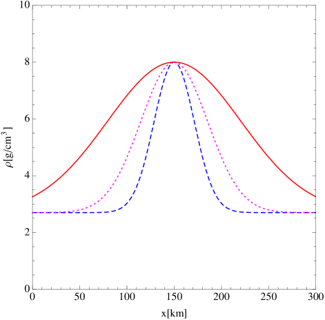
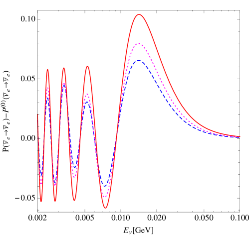
Figure 1: Deviation of neutrino oscillation probability $P(\bar{\nu}_{e}\to\bar{\nu}_{e})$ from the vacuum one (right panel) due to the matter effect of the three different density profiles shown in the left panel. The width of the lump is taken as $D_{l}=100$ km (red solid line), $50$ km (magenta dotted line) and $30$ km (blue dashed line), respectively.

We show in Fig. 1 the deviation of the oscillation probability from the vacuum one as a function of neutrino energy when the lump density is $\rho_{l}=8.0$ g/cm³ that is close to the iron one. It is seen that the deviation changes in accordance with the density profile. This correspondence is the essence of the oscillation tomography. Furthermore, the deviation due to the matter effect is not so large and then the precise measurement of the energy spectrum is a key for the realization of the tomography.

3 Tomography by Neutrino Pair Beam

The strong source of neutrino pairs consisting of $\nu_{\alpha}$ and $\bar{\nu}_{\alpha}$ ($\alpha=e,\mu,\tau$) has been proposed recently [47, 48]. The neutrino pairs are emitted from circulating heavy ions which are in a quantum mixed state $\cos\theta_{c}|g\rangle+e^{-i\epsilon_{eg}t}\sin\theta_{c}|e\rangle$ where the ground state of the ion $|g\rangle$ mixes with its appropriate excited state $|e\rangle$ by the mixing angle $\theta_{c}$. The energy gap of these state is denoted by $\epsilon_{eg}$ and the coherence (mixture) is quantified by $\rho_{eg}=\sin\frac{\theta_{c}}{2}$. The properties of this neutrino pair beam are as follows: the maximal value of the energy sum of neutrino and antineutrino is $E_{m}=2\gamma\epsilon_{eg}$ where $\gamma$ is the Lorentz boost factor of the circulated ions, the beam is well focused for the large $\gamma$ region and the effective angular area is approximately given by $1/\gamma^{2}$, and the spectrum of a neutrino (or an antineutrino) with energy $E_{\nu}$ is given by [47]

$$\frac{d\Gamma}{dE_{\nu}} =\frac{1}{21\times 2^{10}\times\sqrt{6\pi}\,\pi^{4}}aN|\rho_{eg}|^{2}\sqrt{\rho\,\epsilon_{eg}}G_{F}^{2}E_{m}^{4}\frac{1}{\gamma}f(E_{\nu}/E_{m})\,,$$ (27)

where the function $f(x)$ is given by

$$f(x) =\sqrt{x}\int_{0}^{1-x}dyy^{\frac{1}{2}}(y+x)^{\frac{5}{4}}(1-x-y)^{\frac{7}{4}}\,,$$ (28)

and $a$ represents factors of the transition dipole moment and the number of neutrino generations. In this analysis we consider the vector current contribution of neutrino interaction with ionic electron since it gives the oscillation behavior in the probability of the single neutrino detection (while the other neutrino of the pair is undetected) [62]. $N$ and $\rho$ are the number and orbital radius of circulated ions. Note that, when $x\ll 1$, the function $f(x)$ is approximately given by

$$f(x) \simeq 0.0494\sqrt{x}\,.$$ (29)

As representative values we take here $aN|\rho_{eg}|^{2}=10^{8}$, $\gamma=10^{4}$, $\rho=4$ km and $\epsilon_{eg}=50$ keV as in Ref. [47]. In this case the maximum energy is $E_{m}=1$ GeV and the total rate of the pair production is estimated as $5.26\times 10^{16}$ s^-1.

The high intensity $\bar{\nu}_{e}$ beam, called as the beta beam [63], has been proposed. Its flux is much larger than the current accelerator experiments as $2.3$ cm^-2 s^-1. On the other hand, that of the pair beam is estimated as $4.65\times 10^{8}$ cm^-2 s^-1, which clearly shows that the precise measurement of the energy spectrum of the oscillation probability is expected.

In this analysis we consider the detector with liquid argon of fiducial volume $10^{5}$ m³. The signal event is given by the number of the $\bar{\nu}_{e}$ charged current interaction $\bar{\nu}_{e}+p\to e^{+}+n$. The cross section is obtained at low energies

$$\sigma(E_{\nu}) =\frac{|V_{ud}|^{2}E_{\nu}^{2}G_{F}^{2}m_{N}}{3\pi(2E_{\nu}+m_{N})^{3}}\,\Big{[}16(g_{V}^{2}+g_{A}g_{V}+g_{A}^{2})E_{\nu}^{2}+12E_{\nu}m_{N}(g_{V}^{2}+g_{V}g_{A}+2g_{A}^{2})+3m_{N}^{2}(g_{V}^{2}+3g_{A}^{2})\Big{]}$$

$$\simeq 9.34\times 10^{-44}\;\mbox{cm}^{2}\left(\frac{E_{\nu}}{\mbox{MeV}}\right)^{2}~{}~{}\mbox{for}~{}E_{\nu}\ll m_{N}\,,$$ (30)

where $m_{N}$ is a nucleon mass ($m_{N}=m_{p}$), $g_{V}=1$ and $g_{A}=1.2695$. The number of the signal events $N(E_{\nu})$ for the energy region $[E_{\nu},E_{\nu}+\Delta E_{\nu}]$ in the detector located at $L$ from the source is given by

$$N(E_{\nu})\simeq\frac{d\Gamma}{dE_{\nu}}\,\Delta E_{\nu}\,\frac{\gamma^{2}}{4\pi L^{2}}\,P(E_{\nu},L)\,\sigma(E_{\nu})\,n_{N}\,V_{d}\,T\,,$$ (31)

where $V_{d}$ and $n_{N}$ is the volume and the nucleon density of the detector and $T$ is the duration of the observation. Here the area of the detector is assumed to be smaller than $4\pi L^{2}/\gamma^{2}$. It is then for $E_{\nu}\ll E_{m}$ that

$$N(E_{\nu})\simeq 4.73\times 10^{7}\times P(\bar{\nu}_{e}\to\bar{\nu}_{e};E_{\nu})\left(\frac{E_{\nu}}{100~{}\mbox{MeV}}\right)^{\frac{5}{2}}\left(\frac{\Delta E_{\nu}}{1~{}\mbox{MeV}}\right)\left(\frac{300~{}\mbox{km}}{L}\right)^{2}\left(\frac{V_{d}}{10^{5}~{}\mbox{m}^{3}}\right)\left(\frac{T}{1~{}\mbox{year}}\right)\,.$$ (32)

Here we have used the facts that, although the beam produces the pairs of neutrino and antineutrino with all flavors through the charged and neutral current interactions, the dominant one is the pairs of $\nu_{e}$ and $\bar{\nu}_{e}$, and that the detection probability of $\bar{\nu}_{e}$ (while the other $\nu_{e}$ of the pair is undetected) is approximately given by the neutrino oscillation probability $P(\bar{\nu}_{e}\to\bar{\nu}_{e};E_{\nu})$ [62]. It is seen that a large number of $\bar{\nu}_{e}$ events can be detected even at $L=300$ km.

In order to show the significance of the use of the neutrino pair beam quantitatively, we perform the $\chi^{2}$ analysis and show how precise the width and density of the lump can be reconstructed when the density profile is given by Eq. (26). We consider the case when the energy spectrum is measured for 100 bins ($N_{b}=100$) from $E_{\nu}=2$ MeV to 100 MeV, and $\Delta\chi^{2}$ is introduced by

$$\Delta\chi^{2}=\sum_{i=1}^{N_{b}}\frac{\left[N(E_{i})|_{D_{\ast},\rho_{\ast}}-N(E_{i})|_{D_{l},\rho_{l}}\right]^{2}}{\sigma^{2}(E_{i})}\,,$$ (33)

where the true values of width and density of the lump are taken as $D_{l}=30$ km and $\rho_{l}=8.0$ g/cm³. Here we take into account only the statistical error and $\sigma(E_{i})=\sqrt{N(E_{i})|_{D_{l},\rho_{l}}}$.

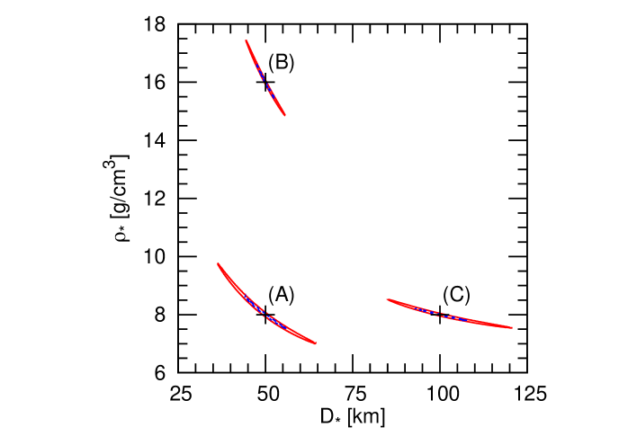
Figure 2: Contour plot of $\Delta\chi^{2}$ in the $D_{*}$-$\rho_{*}$ plane. The true values of the width and density of the lump are taken as (A) $D_{l}=50$ km and $\rho_{l}=8.0$ g/cm³, (B) $D_{l}=50$ km and $\rho_{l}=16$ g/cm³, and (C) $D_{l}=100$ km and $\rho_{l}=8.0$ g/cm³, respectively. $\Delta\chi^{2}=2.3$ ($1\sigma$ level) is shown by blue dashed lines and $\Delta\chi^{2}=11.83$ ($3\sigma$ level) is shown by red solid lines.

In Fig. 2 contour plots of $\Delta\chi^{2}$ in the $D_{*}$-$\rho_{*}$ plane are presented for three different cases. The lines with $\Delta\chi^{2}=2.3$ ($1\sigma$ level) and $\Delta\chi^{2}=11.83$ ($3\sigma$ level) [64] are shown. It is seen that there is an approximate degeneracy between $D_{\ast}$ and $\rho_{*}$. This is because the leading contribution to the oscillation probability from the lump is proportional to the combination $\Delta\rho_{*}\,D_{\ast}$ where $\Delta\rho_{\ast}=\rho_{\ast}-\bar{\rho}$. This degeneracy is broken by the higher order corrections of $\Delta\rho_{*}$ and $D_{\ast}$. The pair beam can probe the lump at the 1 $\sigma$ level as

$$\begin{array}[]{l l c l}\mbox{(A)}&D_{\ast}=50^{+5.9}_{-5.9}~{}\mbox{km}&\mbox{and}&\rho_{\ast}=8.0^{+0.62}_{-0.48}~{}\mbox{g}~{}\mbox{cm}^{-3}\,,\\ \mbox{(B)}&D_{\ast}=50^{+2.5}_{-2.4}~{}\mbox{km}&\mbox{and}&\rho_{\ast}=16^{+0.58}_{-0.53}~{}\mbox{g}~{}\mbox{cm}^{-3}\,,\\ \mbox{(C)}&D_{\ast}=100^{+8.2}_{-7.1}~{}\mbox{km}&\mbox{and}&\rho_{\ast}=8.0^{+0.22}_{-0.21}~{}\mbox{g}~{}\mbox{cm}^{-3}\,,\end{array}$$ (37)

It is, therefore, found that the neutrino pair beam provides the powerful tool to realize the oscillation tomography. The density and width of the lump can be reconstructed accurately if one takes into account the statistical error only. In order to obtain the realistic precision of the reconstruction we have to include various systematic errors in production, propagation and detection rates as well as the mass squared difference and mixing matrix of neutrinos. This issue is beyond the scope of this analysis.

4 Reconstruction of Density Profile

Next, we turn to discuss the reconstruction procedure of $\rho(x)$. One of the serious problems to perform the reconstruction is the degeneracy of the oscillation probabilities. In two-flavor neutrino case the probability between flavor neutrinos with the density profile $\rho(x)$ is the same as that with $\rho(L-x)$. This means that the measurement of the energy spectrum of the oscillation probability is insufficient for the reconstruction when the density profile is asymmetric, i.e. , $\rho(x)\neq\rho(L-x)$. The reconstruction without ambiguity is possible only for the symmetric density profile with $\rho(x)=\rho(L-x)$. It has been pointed out [54, 32] that this difficulty is absent when one uses the solar and supernova neutrinos to probe the interior of the Earth. This is because the initial neutrinos before entering the Earth are not in the flavor eigenstate but in the mass eigenstate due to the MSW effect.

The tomography by the neutrino pair beam under consideration relies on the oscillation probability of $\bar{\nu}_{e}\to\bar{\nu}_{e}$ as explained in the previous section, and hence we are faced with this problem. In this analysis we merely assume the symmetric profile to avoid it, which is the first step towards the analyses of more complicated profiles.

Another difficulty of the reconstruction is the cost of numerical calculations. To reduce it we would like to propose a method based on the perturbation of matter effects. Other methods will be discussed elsewhere [61]. Notice that the matter effects can be treated perturbatively for [60]

$$\frac{\Delta m^{2}}{2E_{\nu}}>\frac{G_{F}}{\sqrt{2}\,m_{p}}\,\rho\,.$$ (38)

Thus, the matter density and the neutrino energy should be sufficiently small for a given $\Delta m^{2}$.

Our proposed method for the reconstruction is as follows: (i) First, we discretize the neutrino baseline into the $N_{L}$ segments. We take here $N_{L}=60$ as an example. The matter densities at each segment $\rho_{i}=\rho(x_{i})$ ($i=1,2,\cdots,N_{L}$) are taken as free parameters, which will be determined by using the $\chi^{2}$ fit to the energy spectrum of the oscillation probability.

(ii) Second, we also divide the energy range of interest into the $N_{E}$ parts. Here the minimum energy is taken as 2 MeV, which is larger than the threshold energy of $\bar{\nu}_{e}$ for the charged current interaction (see the discussion in the previous section). On the other hand, the maximum energy is taken as 100 MeV which is sufficiently small to justify the perturbative treatment of the matter effects. (See Eq. (38)). Here we divide into the $N_{E}=100$ parts of even intervals.

(iii) Finally, we determine the densities $\rho_{i}$ by minimizing the $\chi^{2}$ function which compares the experimental data $N^{\rm obs}(E_{i})$ for a given density profile $\rho(x)$ with the theoretical predictions $N^{\rm th}(E_{i})$ from unknown $\rho_{i}$. The explicit form of the $\chi^{2}$ function is

$$\chi^{2}=\sum_{i=1,N_{E}}\frac{\big{[}N^{\rm obs}(E_{i})-N^{\rm th}(E_{i})\big{]}^{2}}{\sigma^{2}(E_{i})}\,,$$ (39)

where $\sigma(E_{i})=\sqrt{N^{\rm obs}(E_{i})}$. In this analysis we take the number of signal events in Eq. (31) estimated from the oscillation probability including the precise matter effect as the observation one $N^{\rm obs}(E_{i})$. On the other hand, the theoretical one $N^{\rm th}(E_{i})$ is estimated from the analytical expression of the oscillation probability obtained by the perturbation. The use of the perturbative expression is crucial in reducing the numerical cost to reconstruct $\rho_{i}$.

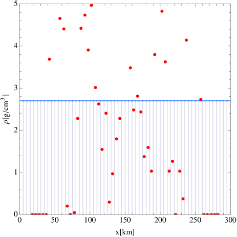
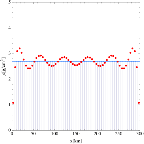
Figure 3: Results of the reconstruction of the flat density profile with $\rho(x)=\bar{\rho}=2.7$ g/cm³. We use the analytic expressions of the energy spectra at the first order (left panel) and the second order (right panel), respectively. The true density profiles are shown by blue lines, while the reconstructed ones are shown by red points.

First of all, we show the results for the case with the flat density profile

$$\rho(x)=\bar{\rho}=2.7~{}\mbox{g/cm}^{3}\,.$$ (40)

As shown in Fig. 3, the reconstruction by using the probability with the first order correction $P^{(1)}(\bar{\nu}_{e}\to\bar{\nu}_{e};E_{\nu})$ is found to be unsuccessful in the present case. On the other hand, when we include the second order correction $P^{(2)}(\bar{\nu}_{e}\to\bar{\nu}_{e};E_{\nu})$, the density profile can be reconstructed within a certain error. It is found that the precision of the reconstruction is ${\cal O}$(10) % except for the regions near the production and detection points.

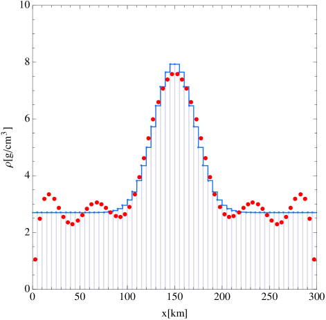
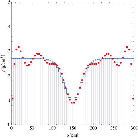
Figure 4: Results of the reconstruction of the two density profiles. The density at the center is $\rho=8$ g/cm³ that is for iron (left panel) and 1 g/cm³ for water (right panel). The true density profiles are shown by blue lines, while the reconstructed ones are shown by red points.

Next, we perform the reconstruction of the density profile with a bump or a dip by using the second order expression. The results are shown in Fig. 4. The density at the center for the bump is taken as 8 g/cm³ which is close to the value for iron, and that for the dip is 1 g/cm³ which is for water (with a pressure of one atmosphere). It is seen that the profiles can be reconstructed well except for the regions near the production and detection points.

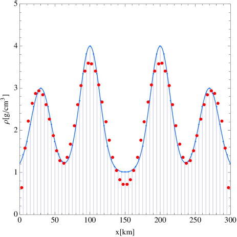
Figure 5: Result of the reconstruction of the symmetric density profile. The true density profile is shown by blue line, while the reconstructed one is shown by red points.

We have found that our proposed method at the second order perturbation works successfully. A rather complicated profile can be reconstructed as long as the density profile is symmetric $\rho(x)=\rho(L-x)$. See, for example, Fig. 5. It should be stressed that this method can operate even with the limited numerical cost because of the analytical expression of the oscillation probability.

Finally, we have observed that the minimum energy in the oscillation probability used for the reconstruction is important to obtain a better result. In the present analysis we take 2 MeV because of the threshold energy of the $\bar{\nu}_{e}$ detection process. As the minimum energy becomes smaller, the result of the reconstruction becomes better. We have found in such cases that the reconstructed densities even near the production and detection points become close to the true values. In addition, the oscillatory behavior of the reconstructed profile at the flat density region becomes changed so that both amplitude (deviation) and wavelength (interval) become smaller, which leads to the better fit. In other words, the main source of the gap from the true profile might be the fact that we can use the oscillation probability for the limited energy range. Especially, those at low energies give a precise information of the density profile. Moreover, the corrections of matter effect at higher orders are also the source of errors in the reconstruction.

5 Conclusions

We have investigated the oscillation tomography using the neutrino pair beam. It has been shown that the beam can offer the powerful neutrino source to probe the Earth’s interior and the precision of the reconstruction of the density profile becomes improved considerably. In addition, we have proposed the tomography method based on the perturbation of matter effects in the oscillation probabilities. This method works only for the symmetric profile with $\rho(x)=\rho(L-x)$ under the situation we have discussed. It has been demonstrated that the profile can be reconstructed well by including the second order correction. We believe that these two ingredients give considerable progress toward the realization of the neutrino tomography.

References

- [1] See, for example, I. Esteban, M. C. Gonzalez-Garcia, M. Maltoni, I. Martinez-Soler and T. Schwetz, JHEP 1701 (2017) 087 [arXiv:1611.01514 [hep-ph]].
- [2] C. Giunti and C. W. Kim, “Fundamentals of neutrino physics and astrophysics”, Oxford University Press (2007).
- [3] A. Placci and E. Zavattini, CERN report, October 1973.
- [4] L. V. Volkova and G. T. Zatsepin, Bull. Acad. Sci. USSR, Phys. Ser. 38 (1974) 151.
- [5] I.Nadyalkov, Acad. Bulgarian Sci. 34 (1981) 177–180.
- [6] I.Nadyalkov, Acad, Bulgarian Sci. 36 (1983) 1515–1518.
- [7] A. De Rujula, S. L. Glashow, R. R. Wilson and G. Charpak, Phys. Rept. 99 (1983) 341.
- [8] T. L. Wilson, Nature 309 (1984) 38.
- [9] G. A. Askarian, Sov. Phys. Usp. 27 (1984) 896 [Usp. Fiz. Nauk 144 (1984) 523].
- [10] L. V. Volkova, Nuovo Cim. C 8 (1985) 552.
- [11] V. A. Tsarev, Sov. Phys. Usp. 28 (1985) 940.
- [12] A. B. Borisov, B. A. Dolgoshein and A. N. Kalinovsky, Yad. Fiz. 44 (1986) 681.
- [13] A. B. Borisov and B. A. Dolgoshein, Phys. Atom. Nucl. 56 (1993) 755 [Yad. Fiz. 56N6 (1993) 78].
- [14] C. Kuo, et al., Earth Plan. Sci. Lett. 133 (1995) 95.
- [15] P. Jain, J. P. Ralston and G. M. Frichter, Astropart. Phys. 12 (1999) 193 [hep-ph/9902206].
- [16] J. P. Ralston, P. Jain and G. M. Frichter, astro-ph/9909038.
- [17] S. Razzaque, P. Meszaros and E. Waxman, Phys. Rev. D 68 (2003) 083001 [astro-ph/0303505].
- [18] M. M. Reynoso and O. A. Sampayo, Astropart. Phys. 21 (2004) 315 [hep-ph/0401102].
- [19] M. C. Gonzalez-Garcia, F. Halzen, M. Maltoni and H. K. M. Tanaka, Phys. Rev. Lett. 100 (2008) 061802 [arXiv:0711.0745 [hep-ph]].
- [20] E. Borriello et al., JCAP 0906 (2009) 030 [arXiv:0904.0796 [astro-ph.EP]].
- [21] N. Takeuchi, Earth, Planets and Space 62, 215 (2010).
- [22] I. Romero and O. A. Sampayo, Eur. Phys. J. C 71 (2011) 1696.
- [23] A. Donini, S. Palomares-Ruiz and J. Salvado, arXiv:1803.05901 [hep-ph].
- [24] V. K. Ermilova, V. A. Tsarev and V. A. Chechin, Bull. Lebedev Phys. Inst. 1988N3 (1988) 51 [Bull. Lebedev Phys. Inst. 3 (1988) 51].
- [25] A. Nicolaidis, Phys. Lett. B 200 (1988) 553.
- [26] A. Nicolaidis, M. Jannane and A. Tarantola, J. Geophys. Res. Solid Earth 96 (1991) 21811.
- [27] T. Ohlsson and W. Winter, Phys. Lett. B 512 (2001) 357 [hep-ph/0105293].
- [28] T. Ohlsson and W. Winter, Europhys. Lett. 60 (2002) 34 [hep-ph/0111247].
- [29] A. N. Ioannisian and A. Y. Smirnov, hep-ph/0201012.
- [30] M. Lindner, T. Ohlsson, R. Tomas and W. Winter, Astropart. Phys. 19 (2003) 755 [hep-ph/0207238].
- [31] W. Winter, Phys. Rev. D 72 (2005) 037302 [hep-ph/0502097].
- [32] E. K. Akhmedov, M. A. Tortola and J. W. F. Valle, JHEP 0506, 053 (2005) [hep-ph/0502154].
- [33] H. Minakata and S. Uchinami, Phys. Rev. D 75 (2007) 073013 [hep-ph/0612002].
- [34] W. Winter, Earth Moon Planets 99 (2006) 285 [physics/0602049].
- [35] R. Gandhi and W. Winter, Phys. Rev. D 75 (2007) 053002 [hep-ph/0612158].
- [36] B. Wang, Y. Z. Chen and X. Q. Li, Chin. Phys. C 35 (2011) 325 [arXiv:1001.2866 [hep-ph]].
- [37] S. K. Agarwalla, T. Li, O. Mena and S. Palomares-Ruiz, arXiv:1212.2238 [hep-ph].
- [38] C. A. Argüelles, M. Bustamante and A. M. Gago, Mod. Phys. Lett. A 30 (2015) no.29, 1550146 [arXiv:1201.6080 [hep-ph]].
- [39] M. A. Millhouse and D. C. Latimer, Am. J. Phys. 81 (2013) 646.
- [40] A. N. Ioannisian, A. Y. Smirnov and D. Wyler, Phys. Rev. D 92 (2015) no.1, 013014 [arXiv:1503.02183 [hep-ph]].
- [41] C. Rott, A. Taketa and D. Bose, Sci. Rep. 5 (2015) 15225 [arXiv:1502.04930 [physics.geo-ph]].
- [42] W. Winter, Nucl. Phys. B 908 (2016) 250 [arXiv:1511.05154 [hep-ph]].
- [43] S. Bourret et al. [KM3NeT Collaboration], J. Phys. Conf. Ser. 888 (2017) no.1, 012114 [arXiv:1702.03723 [physics.ins-det]].
- [44] A. N. Ioannisian and A. Y. Smirnov, Phys. Rev. D 96 (2017) no.8, 083009 [arXiv:1705.04252 [hep-ph]].
- [45] A. D. Fortes, I. G. Wood, and L. Oberauer, Astron. Geophys. 47(2006) 5.31–5.33.
- [46] R. Lauter, Astron. Nachr. 338 (2017) no.1, 111.
- [47] M. Yoshimura and N. Sasao, Phys. Rev. D 92 (2015) no.7, 073015 [arXiv:1505.07572 [hep-ph]].
- [48] M. Yoshimura and N. Sasao, Phys. Rev. D 93 (2016) no.11, 113018 [arXiv:1512.06959 [hep-ph]].
- [49] A. de Gouvea, Phys. Rev. D 63 (2001) 093003 [hep-ph/0006157].
- [50] T. Miura, E. Takasugi, Y. Kuno and M. Yoshimura, Phys. Rev. D 64 (2001) 013002 [hep-ph/0102111].
- [51] E. K. Akhmedov, P. Huber, M. Lindner and T. Ohlsson, Nucl. Phys. B 608 (2001) 394 [hep-ph/0105029].
- [52] T. K. Kuo and J. T. Pantaleone, Phys. Lett. B 198 (1987) 406.
- [53] H. Minakata and S. Watanabe, Phys. Lett. B 468 (1999) 256 [hep-ph/9906530].
- [54] E. K. Akhmedov, M. A. Tortola and J. W. F. Valle, JHEP 0405 (2004) 057 [hep-ph/0404083].
- [55] L. Wolfenstein, Phys. Rev. D 17 (1978) 2369.
- [56] S. P. Mikheev and A. Y. Smirnov, Sov. J. Nucl. Phys. 42 (1985) 913 [Yad. Fiz. 42 (1985) 1441].
- [57] S. P. Mikheev and A. Y. Smirnov, Nuovo Cim. C 9 (1986) 17.
- [58] B. Pontecorvo, Sov. Phys. JETP 7 (1958) 172.
- [59] Z. Maki, M. Nakagawa and S. Sakata, Prog. Theor. Phys. 28 (1962) 870.
- [60] A. N. Ioannisian and A. Y. Smirnov, Phys. Rev. Lett. 93 (2004) 241801 [hep-ph/0404060].
- [61] T. Asaka and H. Okui, in preparation.
- [62] T. Asaka, M. Tanaka and M. Yoshimura, Phys. Lett. B 760 (2016) 359 [arXiv:1512.08076 [hep-ph]].
- [63] P. Zucchelli, Phys. Lett. B 532 (2002) 166.
- [64] C. Patrignani et al. [Particle Data Group], Chin. Phys. C 40 (2016) no.10, 100001, and 2017 update.
- [65] A. Gando et al. [KamLAND Collaboration], Phys. Rev. D 88 (2013) no.3, 033001 [arXiv:1303.4667 [hep-ex]].