Robust Nonparametric Regression under
Huber’s $\epsilon$-contamination Model

Abstract

We consider the non-parametric regression problem under Huber’s $\epsilon$-contamination model, in which an $\epsilon$ fraction of observations are subject to arbitrary adversarial noise. We first show that a simple local binning median step can effectively remove the adversary noise and this median estimator is minimax optimal up to absolute constants over the Hölder function class with smoothness parameters smaller than or equal to 1. Furthermore, when the underlying function has higher smoothness, we show that using local binning median as pre-preprocessing step to remove the adversarial noise, then we can apply any non-parametric estimator on top of the medians. In particular we show local median binning followed by kernel smoothing and local polynomial regression achieve minimaxity over Hölder and Sobolev classes with arbitrary smoothness parameters. Our main proof technique is a decoupled analysis of adversary noise and stochastic noise, which can be potentially applied to other robust estimation problems. We also provide numerical results to verify the effectiveness of our proposed methods.

1 Introduction

Nonparametric regression has a wide range of applications in statistics and machine learning research (Larry, 2006; Tsybakov, 2009; Friedman et al., 2001). In this paper we restrain ourselves to the fixed design setting, where design points $x_{\mathbf{i}}=\left[\frac{i_{1}}{p},\ldots,\frac{i_{d}}{p}\right]$, $i_{1},i_{2},\ldots,i_{d}=1,\cdots,p$ are evenly spaced on $[0,1]^{d}$ and in total we have $n=p^{d}$ design points. In the standard setting, we observe $y_{\mathbf{i}}=f(x_{\mathbf{i}})+\xi_{\mathbf{i}}$ where $f:[0,1]^{d}\to\mathbb{R}$ is an underlying function to be estimated and $\{\xi_{\mathbf{i}}\}$ are i.i.d. noise variables. The objective is to construct an estimate $\widehat{f}$ that is close to $f$ under certain error metric like the mean square error: $\|\widehat{f}-f\|_{2}^{2}:=\int_{[0,1]^{d}}\left|\widehat{f}(x)-f(x)\right|^{2}dx.$

The nonparametric regression problem has a long history of study, dating back to the 1920s (Whittaker, 1922). A large family of methods have been developed and their properties analyzed, including kernel smoothing (Friedman et al., 2001; Györfi et al., 2006), spline smoothing (Reinsch, 1967; Geer, 2000; Green and Silverman, 1993), wavelet smoothing (Donoho et al., 1998; Donoho and Johnstone, 1994; Härdle et al., 2012) and local regression methods (Fan and Gijbels, 1992; Fan, 1993; Fan and Gijbels, 1996). We refer the readers to the excellent books of (Györfi et al., 2006; Tsybakov, 2009; Larry, 2006) for the comprehensive literature on the nonparametric regression problem.

In many real world applications, the observations may subject to systematic or even adversarial noise. Classically, the sensitivity of conventional statistical procedures to outliers was noted by Tukey (1975) who observed that estimators like the empirical mean can be sensitive to even a single gross outlier. In the nonparametric setting, similarly, the adversary noise can completely break these nonparametric estimators.

The formal study of robust estimation was initiated by Huber et al. (1964, 1965), who considered the $\epsilon$-contamination model where the observations are distributed from the mixture:

$$y_{\mathbf{i}}\overset{i.i.d.}{\sim}(1-\epsilon)P(x_{\mathbf{i}})+\epsilon Q(x_{\mathbf{i}}).$$

Here $P\left(\mathbf{x}_{\mathbf{i}}\right)=N(f(x_{\mathbf{i}}),1)$, Gaussian distribution with mean $f(x_{\mathbf{i}})$ and variance $1$, $Q(x_{\mathbf{i}})$ is an arbitrarily adversary distribution and $\epsilon$ is the expected fraction of adversarial outliers.

The performance of robust estimators can be evaluated under a minimax framework recently formulated in the statistics literature (Chen et al., 2015, 2016; Gao, 2017; Liu and Gao, 2017). Typically, the minimax rates under the Huber’s $\epsilon$-contamination model can be divided into two components: (1) The contamination dependence, which concerns the dependence of the estimation error on the contamination parameter $\epsilon$; (2) The statistical rate, which coincides with the classical notion of statistical consistency and goes to zero as we accumulate more data (i.e., $n\to\infty$). We say a robust estimator is minimax optimal if both its contamination dependence and statistical rate match their information-theoretical limits, up to absolute constants.

Our contributions:

In this paper, we present a simple and easy-to-compute local binning median method which can effectively remove all the adversarial noise. Theoretically, this method is statistically optimal in terms of both contamination dependency and statistical rate up to absolute constant for estimating functions in Hölder class with smoothness parameter $\beta\in[0,1]$ (a formal definition of Hölder function class is given in Sec. 1.2).

Furthermore, we propose a generic method for estimating functions with higher orders of smoothness. Our method has two steps. First, we use a local binning median estimator to remove adversarial noise. Next, we take a non-parametric procedure on top of these medians where the specific choice of the procedure depends on user’s knowledge of the underlying function. In particular, we show that if we use kernel smoothing or local polynomial regression, we can achieve minimaxity for Hölder and Sobolev function classes with higher orders of smoothness. We remark that both steps can be computed efficiently in polynomial time.

To our knowledge, these are the first computationally efficient algorithms for nonparametric regression under the Huber’s $\epsilon$-contamination model with provably optimal contamination dependency and statistical rate.

1.1 Related work

Some of the classical literature on robust statistics focused on the design of robust estimators and the study of their statistical properties (see, for instance, the works of  Huber (2011); Hampel et al. (2011)). The major drawback of many of these classical robust estimators is that they are either heuristic in nature (for instance, methods based on Winsorization (Hastings Jr et al., 1947) are generally not optimal in the minimax sense), or are computationally intractable (for instance, methods based on Tukey’s depth (Tukey, 1975) or on $\ell_{1}$ tournaments (Yatracos et al., 1985)).

In the nonparametric setting, most papers focused on density estimation problems (Acharya et al., 2017; Chan et al., 2014; Diakonikolas et al., 2016b; Daskalakis et al., 2012; Liu and Gao, 2017). On the other hand, existing works on robust nonparametric regression only focused on heavy-tailed noise (Fan et al., 1994), but not Huber’s $\epsilon$-contamination model. To our knowledge, only Gao (2017) considered nonparametric regression problems in this model. This estimator is based on the concept of regression depth, a generalization of Tukey’s depth and achieves optimal contamination dependency and statistical rate for Sobolev function class. Unfortunately, there is no known polynomial time algorithm to compute such estimators.

Methodologically, our proposed algorithms also resemble the two-step method considered in (Brown et al., 2008). However, their analysis is based on asymptotic equivalence (Cai et al., 2009) and cannot be adapted to Huber’s $\epsilon$-contamination model. Instead, we propose a decoupled analysis and only use elementary concentration inequalities to prove the upper bound of this estimator. Given the importance of Huber’s $\epsilon$-contamination model, we believe our proof techniques can also be used in other robust statistical estimation problems.

Recent works from the theoretical computer science community proposed new methods for robust statistical estimation with polynomial running time guarantees. Diakonikolas et al. (2016a); Lai et al. (2016); Charikar et al. (2017) provide some of the first computationally tractable, provably robust estimators with near-optimal contamination dependence in a variety of settings. More recently, generalization to high-dimensional setting (Balakrishnan et al., 2017) is also studied. However, these works only focused on the parametric models.

1.2 Function Classes

The Hölder class is a popular choice of smoothness classes for nonparametric estimation problems. The following definition gives a rigorous mathematical formulation of Hölder classes considered in this paper:

Definition 1.

For $f:\left[0,1\right]^{d}\rightarrow\mathbb{R}$, if $f\in\Lambda\left(\beta,L\right)$, then it satisfies for any $x,x^{\prime}\in\left[0,1\right]^{d}$

$$\sum_{j=0}^{\ell}\sum_{\alpha_{1}+\cdot+\alpha_{d}=j}\left|f^{(\mathbf{\alpha},j)}(x)\right|+\sum_{\alpha_{1}+\cdots+\alpha_{d}=k}\frac{\left|f^{(\mathbf{\alpha},k)}(x)-f^{(\mathbf{\alpha},k)}(x^{\prime})\right|}{\left\|x-x^{\prime}\right\|_{\infty}^{\beta-\ell}}\leq L$$

where $\ell=\lfloor\beta\rfloor$ and $f^{(\mathbf{\alpha},j)(x)}=\partial^{j}f(x)/\partial x_{1}^{\alpha_{1}}\ldots\partial x_{d}^{\alpha_{d}}$.

At a higher level, functions belonging to the Hölder class have their derivatives and derivative changes uniformly bounded on the unit interval $[0,1]^{d}$.

While Hölder class imposes uniform smoothness condition, Sobolev class only assumes the averaged magnitudes of the derivatives are bounded. Here we adopt the definition from Nemirovski (2000).

Definition 2.

For $f:\left[0,1\right]^{d}\rightarrow\mathbb{R}$, if $f\in\Sigma\left(\beta,p,L\right)$, it satisfies

$$\left\|D^{\beta}f\right\|_{p}\leq L$$

where $\beta\geq 1$, $p\geq d$ are integers and $D^{\beta}f(\cdot)$is the vector function comprised of all partial derivatives (in terms of distributions) of f with order $\beta$.

2 Some Natural Approaches and Their Problems

In this section we discuss some natural approaches and their problems. For the ease of presentation we focus on the one dimensional setting.

Example I: Direct Kernel Smoothing

We first consider directly applying kernel smoothing estimator to this problem. Let $x_{0}$ be a query point, recall the kernel smoothing method has the following weighted sum form :$\widehat{f}(x_{0})=\sum_{i=1}^{n}\frac{1}{h}K_{i}^{h}(x_{0})y_{i}.$ where $K_{i}^{h}(\cdot)$ is a kernel function and $h$ is the band-width. Consider the case that there exists some $i$ such that $K_{i}^{h}(x_{0})>0$ and $\xi_{i}\sim Q$, the noise is sampled from the adversarial distribution. Because $Q$ is arbitrary, $\xi_{i}$ can be infinity and in turn $y_{i}$ is infinity. Therefore, in this situation our estimator will output infinity which is undesirable. One may think this event happens with low probability. However, note for every observation $y_{i}$ we have $\epsilon$ probability that $\xi_{i}\sim Q$. Thus it is not hard to show with high probability that there exists one $i$ such $K_{i}^{h}(x_{0})>0$ and $y_{i}=\infty$.

Example II: Truncated Kernel Smoothing

A natural to deal with the extremely large adversarial noise is to use truncation. For Hölder class, since we know $\left\|f\right\|_{\infty}\leq L$ and $P$ is standard Gaussian distribution. We can modify the kernel smoothing estimator as $\widehat{f}(x_{0})=\sum_{i=1}^{n}\frac{1}{h}K_{i}^{h}(x_{0})\overline{y}_{i}$ where

$$\overline{y}_{i}=\begin{cases}L+c\text{ if }y_{i}\geq L+c\\ y_{i}\text{ if }-(L+c\sigma)\leq y_{i}\leq L+c\\ -(L+c)\text{ if }y_{i}\leq-(L+c)\end{cases}.$$

Here we choose $c>1$ to ensure most samples whose noise are from $P$ are not being truncated (Diakonikolas et al., 2016a). This estimator rules out the infinite issue. However, consider the following scenario. Let $x_{0}$ be a query point and $f(x_{0})=0$. Note around $x_{0}$ there are approximately $\epsilon$ adversarial observations and if we set the adversarial distribution to be a unit mass on the infinity, then there are approximately $\epsilon$ fraction of $\overline{y}_{i}$s are $L+c$. These points will incur an $\Omega\left(\epsilon^{2}(L+1)^{2}\right)$ squared bias in our estimation. In Section 5, we will show the optimal lower bound for the contamination dependency is $\Omega\left(\epsilon^{2}\right)$ and it does not depend on $L$. When $L$ is relatively large, this estimation will be far off from the truth. We also verify this phenomenon by simulation in Section 6.

3 Local Binning Median Estimator

We introduce the local binning estimator and its theoretical properties in this section. The interval $\left[0,1\right]$ is evenly divided into $m$ sub-intervals. The bin $\mathbf{j}=\left(j_{1},\ldots,j_{d}\right)$ corresponds to the $d$-dimensional box $[\frac{j_{1}-1}{m},\frac{j_{1}}{m})\times\cdots\times[\frac{j_{d}-1}{m},\frac{j_{d}}{m})$ and has $s=\frac{n}{m^{d}}$ design points. For a query point $x_{0}\in[0,1]^{d}$, let $\mathbf{j}\in[m]$ be the label of the unique bin that contains $x_{0}$. The local binning median estimator evaluated at $x_{0}$ is then defined as

$$\widehat{f}\left(x_{0}\right):=\mathrm{median}\left\{y_{\mathbf{i}}\right\}_{\mathbf{i}\in\text{ bin }\mathbf{j}}.$$

where $\mathbf{i}=\left(i_{1},\ldots,i_{d}\right)$ is the index. It is clear that $\widehat{f}(x_{0})$ is easily computed in time $O(s)$, as the median can be computed in linear time (see, e.g., Kleinberg and Tardos (2006)).

Before delving into detailed statistical properties $\widehat{f}$, we provide motivations for both the median operator and the local binning approach taken in $\widehat{f}$.

The median.

Median is widely used in robust estimation problems for dealing with adversarial noise (Huber, 2011), heavy tail noise (Brown et al., 2008), etc. There are two fundamentally useful properties about median. First, taking the median ensures that, as long as the majority of the samples are good, the output will not be affected by the small amount of outliers. In addition, the median itself has an concentration effect similar to what the mean does. Our proof heavily relies on these two properties.

The local binning.

Binning is used to exploit the smoothness of the function class. Since the binning estimator only uses observations near the query point, for smooth function class, this estimator will incur only a small bias. This is the same idea in kernel smoothing where we often put more weights on points that are near the query point.

We are ready ready to state our main lemma which characterizes the performance of this local binning median estimator.

Lemma 1.

Suppose $\epsilon\leq 1/4$. Let $s=\frac{n}{m^{d}}$ and $z_{\mathbf{j}}=\mathrm{median}\left\{y_{\mathbf{i}}\right\}_{\mathbf{i}\in\text{ bin }\mathbf{j}}$. With probability at least 0.9, for any $\mathbf{j}\in[m]^{d}$, we have

$$z_{\mathbf{j}}=f\left(\frac{\mathbf{j}}{m}\right)+\Delta_{j}+\eta_{j}$$

where $\left|\Delta_{\mathbf{j}}\right|\leq\max_{x\in\text{ bin }\mathbf{j}}\left|f\left(x\right)-f\left(\frac{\mathbf{j}}{m}\right)\right|$, $\left|\mathbf{E}\left[\eta_{\mathbf{j}}\right]\right|\leq C\left(\epsilon+\frac{\log m}{s}\right)$ and $\textbf{Var}\left(\eta_{\mathbf{j}}\right)\leq\frac{C}{s}$.

Lemma 1 shows a form of bias-variance trade-off. $\left|\Delta_{\mathbf{j}}\right|$ characterizes the bias incurred by our binning step. This term is small if the function we are estimating has smoothness property. $\left|\mathbf{E}\left[\eta_{\mathbf{j}}\right]\right|$ characterizes the biased incurred by the adversary and stochastic noise. Later in Section 5, we will show that $\epsilon$ is unavoidable in Huber’s $\epsilon$-contamination model. The $\frac{\log m}{s}$ is small if $s$ is relatively large. Lastly, $\textbf{Var}\left(\eta_{\mathbf{j}}\right)$ is the variance incurred by the stochastic noise. Note we have $\textbf{Var}\left(\eta_{\mathbf{j}}\right)=O\left(\frac{1}{s}\right)$ because the variance of the median of $s$ sub-Gaussian random variable is $O\left(\frac{1}{s}\right)$.

With this meta Lemma at hand, we can direct derive upper bounds for some particular function classes.

Theorem 1 (Estimation Error Bound for Hölder Function Class).

Suppose $f\in\Lambda(\beta,L)$ for some $\beta\in(0,1]$ and $m\asymp n^{\frac{1}{2\beta+d}}L^{\frac{2}{2\beta+d}}$. Then there exists an absolute constant $C>0$ such that with probability at least 0.9,

$$\left\|\widehat{f}-f\right\|_{2}^{2}\leq C\left(L^{\frac{2d}{2\beta+d}}n^{-\frac{2\beta}{2\beta+d}}+\epsilon^{2}\right).$$

Remark 1.

Though Theorem 1 seems to appear only to Hölder class with $\beta\leq 1$, one should note that $\Lambda(\beta,L)\subseteq\Lambda(\beta^{\prime},L)$ always holds for any $\beta\geq\beta^{\prime}$. Therefore, in cases where $\beta>1$, the scaling of $m$ and the upper bound on $\|\widehat{f}-f\|_{2}^{2}$ remain valid with $\beta$ replaced by $\beta^{\prime}=\min\{\beta,1\}$.

Remark 2.

Theorem 1 suggests two potential sources of error in $\|\widehat{f}-f\|_{2}^{2}$. The first term $L^{2d/(2\beta+d)}n^{-2\beta/(2\beta+d)}$ is the classical statistical rate in nonparametric regression and goes to 0 as $n$ increases to infinity. The second term $\epsilon^{2}$ represents the contamination dependency and typically remains constant under large-$n$ asymptotic regimes. Importantly, this term does not depend on the Hölder smooth constant $L$.

4 Post-processing to Exploit Higher Smoothness

While the local binning median estimator $\widehat{f}$ is intuitive, the number of bins $m\asymp n^{\frac{1}{1+2\beta^{\prime}}}L^{\frac{2}{2\beta^{\prime}+1}}$ for $\beta^{\prime}=\min\{\beta,1\}$ is likely to be too large for smoother Hölder functions where $\beta>1$ or Sobolev functions. This leads to under-smoothing and loss of statistical efficiency. The main reason is a simple local median step cannot exploit the smoothness in the derivatives of the underlying function (c.f. Definition 1 and Definition 2).

In this section we show a simple post-processing step can exploit this higher smoothness property. Our main observation is from Lemma 1. Recall we have with high probability

$$z_{\mathbf{j}}=f\left(\frac{\mathbf{j}}{m}\right)+\Delta_{\mathbf{j}}+\eta_{\mathbf{j}}.$$

We view $z_{\mathbf{j}}$ as a noisy observation of $f\left(\frac{\mathbf{j}}{m}\right)$ where the noise is $(\Delta_{\mathbf{j}}+\eta_{\mathbf{j}})$ which has bounded bias $O(\epsilon+\frac{\log m}{s})$ and variance $\frac{1}{s}$. Therefore we can take any algorithm that works for non-parametric problem under stochastic noise with bounded bias. Formally, we define a non-parametric algorithm acting on $n$ samples as a map

$$\mathcal{A}:\mathcal{A}\left(\left\{y_{i}\right\}_{i=1}^{n},x_{0}\right)\rightarrow\widecheck{f}\left(x_{0}\right)$$ (1)

where $x_{0}$ is a query point and $\left\{y_{i}\right\}_{i=1}^{n}$ are observations. The final performance will depend on how the noise affect the algorithm. This abstract procedure is summarized in Algorithm 1

Algorithm 1 The local binning median estimator with post-processing

1:  Input: $\left\{y_{\mathbf{i}}\right\}_{i=1}^{n}$, number of bins $m$, $s=\lfloor n/m^{d}\rfloor$, a nonparametric algorithm $\mathcal{A}$ defined in Equation (1), query point $x_{0}$.

2:  Output: estimated function value $\widecheck{f}(x_{0})$.

3:  for $\mathbf{j}=[m]^{d}$ do

4:     Compute $z_{\mathbf{j}}=\mathrm{median}\left\{y_{\mathbf{i}}\right\}_{i\in\text{ bin }\mathbf{j}}$.

5:  end for

6:  Compute $\widecheck{f}\left(x_{0}\right)=\mathcal{A}\left(\left\{\mathbf{z}_{\mathbf{j}}\right\}_{\mathbf{j}\in[m]^{d}},x_{0}\right)$

Now we use two specific non-parametric estimators to illustrate this idea.

4.1 Post-processing by kernel smoothing

We first choose the non-parametric estimation $\mathcal{A}$ to be kernel smoothing for one dimensional robust non-parametric estimation to illustrate the usage of Algorithm 1. This estimator which significantly improves the statistical efficiency of $\widehat{f}$ for highly smooth functions in the Hölder class. Let $K:\mathbb{R}\to\mathbb{R}^{*}$ be a kernel function selected by the data analyzer. We assume the kernel function $K(\cdot)$ satisfies the following properties:

1. $K$ is supported on $[-1,1]$, and $\int_{-1}^{1}K(x)dx=1$;

2. $\int_{-1}^{1}K(x)x^{k}dx=0$ for all $k=1,\ldots,\ell$;

3. $\int_{-1}^{1}K^{2}(x)dx=:\kappa<\infty$.

We remark that the above assumptions on properties of $K(\cdot)$ are not restrictive, as the choice of the kernel function $K(\cdot)$ belongs to the data analyzer and there are many simple functions satisfying (A1) through (A3) for various values of $\ell$. Examples include the box kernel $K(u)=\mathbb{I}[|u|\leq 1]$, the triangular kernel $K(u)=\max\{0,1-|u|\}$ and the Epanechnikov kernel $K(u)=\max\{0,\frac{3}{4}(1-u^{2})\}$.

Given $0<h<1/2$ and a query point $x\in\left(h,1-h\right)$ we define for $j=1,\ldots,m$,

$$K_{j}^{h}(x)=\int_{(j-1)/m}^{j/m}\frac{1}{h}K\left(\frac{x-u}{h}\right)du.$$ (2)

The kernel smoothing step can then be understood as applying the $K_{j}^{h}(\cdot)$ operator over all observations or their local binning median surrogates and aggregating the results.

The next theorem states the main result for the combined two-step procedure, which shows that $\widecheck{f}$ enjoys improved error convergence for highly smoother functions $f\in\Lambda(\beta,L)$ with $\beta>1$.

Theorem 2.

Suppose $f\in\Lambda(\beta,L)$ for $\beta\in(1,\infty)$ and let $c\in(0,1/2)$ be a small constant. If in Algorithm 1, we choose $\mathcal{A}$ to be the kernel smoothing estimator defined in Equation (2), $m\asymp\sqrt{n}/{\sqrt[4]{\log n}}$ and $h\asymp\left(nL^{2}\right)^{-\frac{1}{2\beta+1}}$, then there exists an absolute constant $C>0$ and a constant $C_{L}>0$ depending on $L$ such that with probability at least 0.9,

$$\int_{c}^{1-c}\left|\widecheck{f}(x)-f(x)\right|^{2}dx\leq C\left(C_{L}n^{-\frac{2\beta}{2\beta+1}}+\epsilon^{2}\right).$$

Remark 3.

Theorem 2 nicely complements the results in Theorem 1 by applying to “smoother” functions $f\in\Lambda(\beta,M)$ with $\beta>1$. The error bound is very similar to the one in Theorem 1, except that the constant in front of the statistical rate term $n^{-2\beta/(2\beta+1)}$ is more involved and we decided to suppress its exact dependency on $L$. The contamination dependency term $\epsilon^{2}$ is again independent of smoothness constant $L$.

Remark 4.

We consider the integrated loss over the interval $[c,1-c]$ to constrains the evaluation of the mean-square error to a strict interior of $(0,1)$ which avoid “boundary effects” of the kernel smoothing estimator.

Remark 5.

It possible to extend kernel smoothing estimator to $d>1$. However, it requires more complicated kernel construction, especially for the fixed design. Therefore, for $d>1$ we consider another estimator, local polynomial regression for estimation.

4.2 Post-processing by Local Polynomial Regression

In this section we choose $\mathcal{A}$ to be a local polynomial regression estimator for multivariate robust nonparametric regression. We let $h$ be a fixed bandwidth parameter. Given a query point $x\in\left[0,1\right]^{d}$, local polynomial regression uses the following least square solution as an estimate of $f$ around $x$

$$\widehat{f}_{h}=\arg\min_{g\in\mathcal{P}_{\ell}}\sum_{\mathbf{j}\in[m]^{d}}\mathbb{I}\left[\frac{\mathbf{j}}{m}\in B_{h}^{\infty}\left(x\right)\right]\left(z_{\mathbf{j}}-g(\frac{\mathbf{j}}{m})\right)^{2}$$ (3)

where $\mathcal{P}_{\ell}$ denotes the set of polynomials with degree $d$, $B_{h}^{\infty}\left(x\right)$ is the a ball with radius $h$ in infinity norn and $\mathbb{I}\left[\cdot\right]$ is the indicator function.

The following theorems show the performance for Hölder and Sobolev class.

Theorem 3.

Suppose $f\in\Lambda(\beta,L)$ for $\beta\in(1,\infty)$ or $f\in\Sigma(\beta,p,L)$ for some positive integer $\beta,p$ that satisfy $\frac{\beta-1}{d}\geq\frac{1}{p}$. If in Algorithm 1, we choose $\mathcal{A}$ to be the local polynomial regression estimator defined in Equation (3), $m\asymp\sqrt{n}/{\sqrt[4]{\log n}}$ and $h\asymp\left(nL^{2}\right)^{-\frac{1}{2\beta+d}}$ then there exists an absolute constant $C>0$ and a constant $C_{L}>0$ depending on $L$ such that with probability at least 0.9,

$$\left\|\widehat{f}-f\right\|_{2}^{2}\leq C\left(C_{L}n^{-\frac{2\beta}{2\beta+d}}+\epsilon^{2}\right).$$

Again this matches the minimax lower bound. The proof is similar to that of Theorem 2 where we just need to combine Lemma 1 and standard analysis of local polynomial regression.

5 Minimax lower bounds

We complement our positive results with the following negative result, which establishes minimax lower bounds for nonparametric estimation over the Hölder and Sobolev function class under the Huber’s $\epsilon$-contamination model.

Theorem 4.

For any $\beta,L>0$ and $\epsilon\in(0,1)$, there exists an absolute constant $C>0$ such that

$$\inf_{\widehat{f}}\sup_{f\in\Lambda\left(\beta,L\right)}\Pr_{f,\epsilon,Q}\left[\|\widehat{f}-f\|_{2}^{2}\ \geq C\left(\wp(L)\cdot n^{-\frac{2\beta}{2\beta+d}}+\epsilon^{2}\right)\right]\geq 1/4,$$

where $\wp(L)$ is a non-zero polynomial function of $L$.

Theorem 5.

Let $\beta,p$ be positive integers and satisfy $\frac{\beta-1}{d}\geq\frac{1}{p}$. For any $\epsilon\in(0,1)$, there exists an absolute constant $C>0$ such that

$$\inf_{\widehat{f}}\sup_{f\in\Sigma\left(\beta,p,L\right)}\Pr_{f,\epsilon,Q}\left[\|\widehat{f}-f\|_{2}^{2}\ \geq C\left(\wp(L)\cdot n^{-\frac{2\beta}{2\beta+d}}+\epsilon^{2}\right)\right]\geq 1/4,$$

where $\wp(L)$ is a non-zero polynomial function of $L$.

Remark 6.

The lower bound can be again divided into two components, with the “statistical rate” component $\wp(L)n^{-2\beta/(2\beta+d)}$ going to zero as $n$ increases to infinity, and the “contamination dependency” term $\epsilon^{2}$ that remains constant and is independent of the smoothness constant $L$.

Remark 7.

The minimax lower bound established in Theorem 4 and 5 matches the upper bounds in Theorems 1, 2 and 3 for both the statistical rate component and the contamination dependency component, up to absolute constants and polynomial functions of $L$. In particular, the contamination dependency is $\epsilon^{2}$ in all theorems without any dependency on the smoothness constant $L$, which demonstrates an interesting “de-coupling” effect between benign and adversarial noise variables.

6 Numerical results

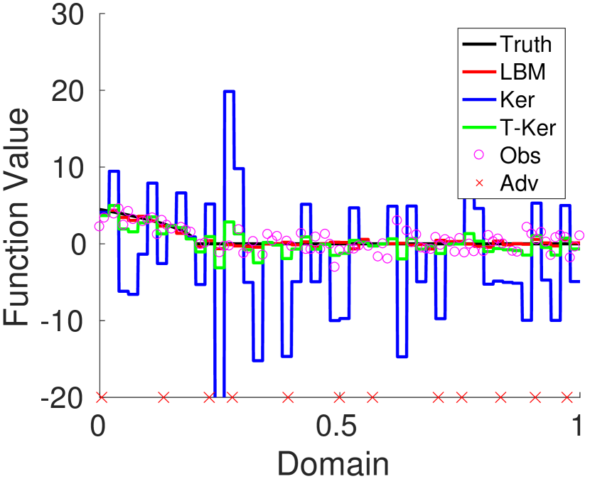
(a) $L=10$

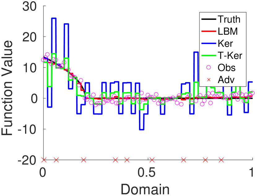
(b) $L=30$

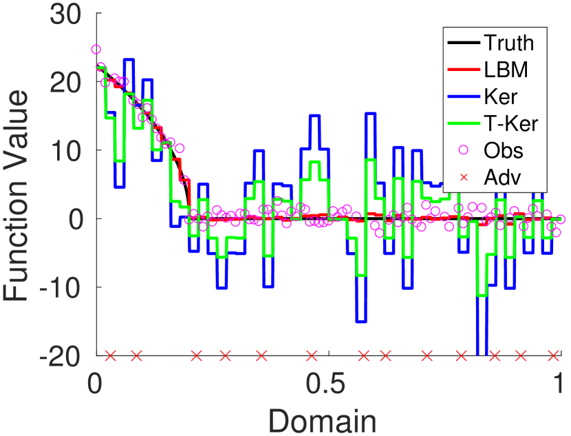
(c) $L=50$

Figure 1: Experiments on estimating a function with low smoothness We choose $\beta=0.5$, $\epsilon=0.1$, $\rho=0.2$ and $f(x)=L(x-\rho)^{\beta}$ for $x\leq\rho$ and $f(x)=0$ otherwise. Red ’X’s represent the positions of adversarial points.

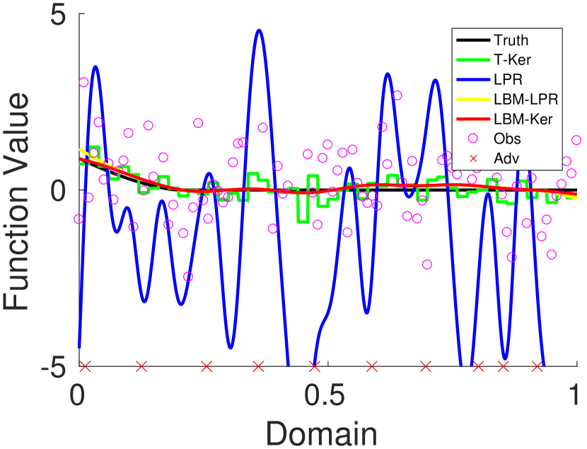
(a) $L=10$

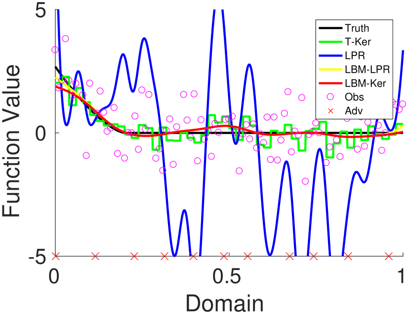
(b) $L=30$

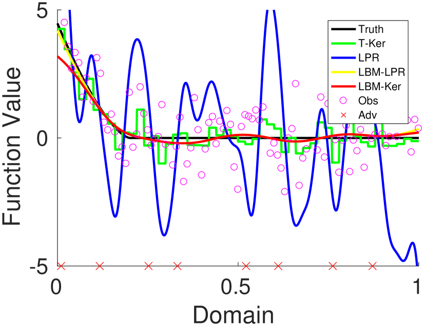
(c) $L=50$

Figure 2: Experiments on estimating a function with high smoothness. We choose $\beta=1.5$, $\epsilon=0.1$, $\rho=0.2$ and $f(x)=L(x-\rho)^{\beta}$ for $x\leq\rho$ and $f(x)=0$ otherwise. Red ’X’s represent the positions of adversarial points.

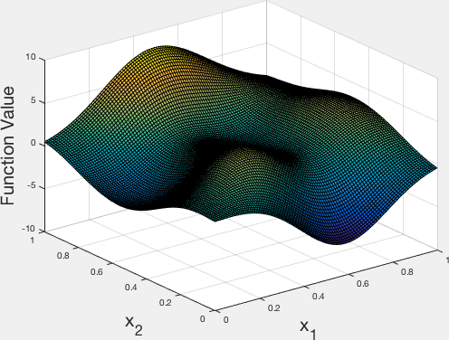
(a) Original Function.

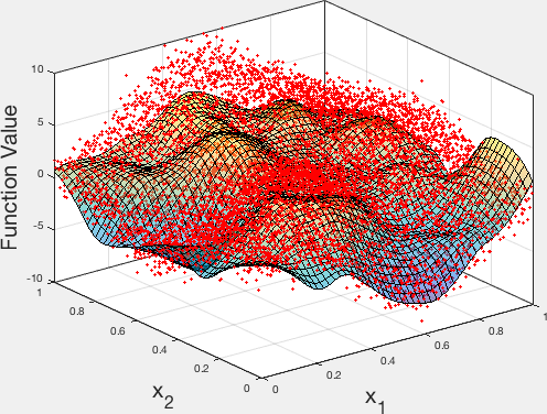
(b) LPR estimator.

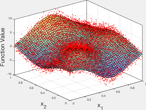
(c) LBM+LPR estimator.

Figure 3: $2$-dimensional nonparametric estimation for peak function.

We first use simulations to verify our theoretical results. In Figure 1-Figure 3, we consider the following estimators: (1) Kernel: the classical kernel smoothing estimator; (2) T-kernel: truncated kernel smoothing estimator described in Section 2. We use an additional hyperparameter $T$ to control the truncation level; (3) LBM: local binning median estimator described in Section 3; (4) LBM+Ker: local binning median estimator with kernel smoothing post-processing described in Section 4; (5) LPR: standard local polynomial regression; (6) LBM+LPR: local binning median estimator with local polynomial regression described in Section 4.2. For all experiments, the hyperparameters are tuned to achieve the best performance. For all figures, we only show 10% observation points for better visualization.

In Figure 1, we consider estimating a one dimensional function with low smoothness. We choose $\beta=0.5$, $\epsilon=0.1$, $\rho=0.2$ and $f(x)=L(x-\rho)^{\beta}$ for $x\leq\rho$ and $f(x)=0$ otherwise. We let $Q$ be a Bernoulli distribution with half probability being $100$ and half probability being $-100$. Figure 1 shows our estimator is consistently better than other estimator. Further when $L$ becomes bigger, truncated kernel estimator has worse performance, verifying our theoretical analysis in Section 2. On the other hand, local binning median estimator is not being affected.

In Figure 2 we compare different estimators for estimating a one dimension function. We use the same setup as in Figure 1 except change the smoothness $\beta$ to $1.5$. In this setting, naive algorithms like LPR and T-Kernel do not perform well while our proposed LBM+LPR and LBM+Ker give significant better results.

In Figure 3, we consider estimating a peak function using direct LPR and LBM+LPR. Note the fitting by LPR is far from the true function whereas the estimation by our proposed LBM + LPR method is close to the truth.

Lastly, in Figure 4 we explore our pre-processing procedure combining with other non-parametric estimator. Here we consider the image denoising task where every pixel is subject to stochastic noise and a small amount of pixels are subject to adversarial noise. Figure 4(a) shows the noisy image. In Figure 4(b) we directly apply Total Variation de-noising algorithm (Rudin et al., 1992). However, due to the adversarial noise, there are still noisy points in the output image. In Figure 4(c), we first use local binning median then apply Total Variation de-noising algorithm. Here, we successfully remove all adversarial noise.

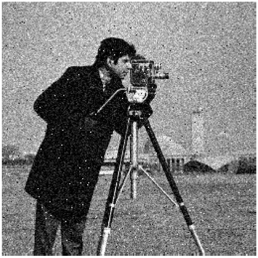
(a) Noisy image. White points on the coat and black points in the background are adversarial points.

(b) Direct total variation de-noising.

(c) Local binning median followed total variation de-noising.

Figure 4: Experimetns on image denoising.

Appendix A Proofs

A.1 Useful Lemmas

We first establish the following lemma that provides the key bias-variance decomposition of the local binning median estimator. The main component is a deterministic analysis on the median and the noise structure.

Lemma 2.

Denote $z_{\mathbf{j}}=\mathrm{median}\left\{y_{\mathbf{i}}\right\}_{\mathbf{i}\in\text{ bin }\mathbf{j}}$ as the median estimator in the bin $\mathbf{j}$. Then $z_{\mathbf{j}}$ can be written as $z_{\mathbf{j}}=f(\mathbf{j}/m)+\eta_{\mathbf{j}}+\Delta_{\mathbf{j}}$, where

• $\eta_{\mathbf{j}}=\mathrm{median}\left\{\xi_{\mathbf{i}}\right\}_{\mathbf{i}\in\text{ bin }\mathbf{j}}$ where $\xi_{\mathbf{i}}\sim(1-\epsilon)N(0,1)+\epsilon(Q(x_{\mathbf{i}})-f(\frac{\mathbf{i}}{n}))$, and

• $\left|\Delta_{\mathbf{j}}\right|\leq\max_{\mathbf{i}\in\text{ bin }\mathbf{j}}\left|f(\frac{\mathbf{i}}{n})-f(\frac{\mathbf{j}}{n})\right|$ almost surely.

To prove Lemma 2, we need the following sandwiching inequality for the median operator.

Proposition 1.

For any sequences $\{a_{i}\}_{i}$ and $\{b_{i}\}_{i}$ of equal length, it holds that $\min\{a_{i}\}_{i}\leq\mathrm{median}\{a_{i}+b_{i}\}_{i}-\mathrm{median}\{b_{i}\}_{i}\leq\max\{a_{i}\}_{i}.$

Proof.

$$\mathrm{median}\left(\left\{Y_{i}\right\}_{i=1}^{m}\right)-\mathrm{median}\left(\left\{\xi_{i}\right\}_{i=1}^{m}\right)$$

$$= \mathrm{median}\left(\left\{Z_{i}+\xi_{i}\right\}_{i=1}^{m}\right)-\mathrm{median}\left(\left\{\xi_{i}\right\}_{i=1}^{m}\right)$$

$$\geq \mathrm{median}\left(\min Z_{i}+\left\{\xi_{i}\right\}_{i=1}^{m}\right)-\mathrm{median}\left(\left\{\xi_{i}\right\}_{i=1}^{m}\right)$$

$$= \min Z_{i}.$$

Using similar argument we can prove the other direction. ∎

Proof of Lemma 2.

Recall we can write the observation model as

$$y_{\mathbf{i}}=f(\mathbf{i}/n)+\xi_{\mathbf{i}}$$

where $\xi_{i}\sim\left(1-\epsilon\right)N\left(0,1\right)+\epsilon Q\left(x_{\mathbf{i}}-f(\frac{\mathbf{i}}{n})\right)$. Therefore,

$$y_{\mathbf{i}}-f(\mathbf{j}/m)=\left(f(\mathbf{i}/n)-f(\mathbf{j}/m)\right)+\xi_{\mathbf{i}}.$$

Denote $\eta_{\mathbf{j}}=\mathrm{median}\left\{\xi_{i}\right\}_{\mathbf{i}\in\text{ bin }\mathbf{j}}$. Applying Proposition 1 and noting that $z_{\mathbf{j}}=\mathrm{median}\{y_{i}\}_{\mathbf{i}\in\text{ bin }\mathbf{j}}$, we have

$$\min_{\mathbf{i}\in\text{ bin }\mathbf{j}}f\left(\mathbf{i}/n\right)\leq z_{\mathbf{j}}-\eta_{\mathbf{j}}\leq\max_{\mathbf{i}\in\text{ bin }\mathbf{j}}f\left(\mathbf{i}/n\right).$$

Define $\Delta_{\mathbf{j}}=z_{\mathbf{j}}-\eta_{\mathbf{j}}-f\left(\frac{\mathbf{j}}{m}\right)$. We have

$$\left|\Delta_{j}\right|\leq\max_{\mathbf{i}\in\text{ bin }\mathbf{j}}\left|f(\mathbf{i}/n)-f(\mathbf{j}/m)\right|$$

almost surely. The lemma is thus proved. ∎

To analyze $\eta_{\mathbf{j}}$, we use a decoupled analysis for the adversarial noise and the stochastic noise. Suppose out of the $s$ samples in the $\mathbf{j}$-th bin, $s_{\mathbf{j}}$ observations come from the adversarial noise distribution $Q$. Our key lemma shows that if $s_{\mathbf{j}}\leq s/4$, these adversarial observations incur a small amount of additional bias in the median over $\{\xi_{\mathbf{i}}\}_{\mathbf{i}\in\text{ bin }\mathbf{j}}$.

Lemma 3.

Suppose $0\leq s^{\prime}<s/4$. Let $\widetilde{\xi}_{1},\ldots,\widetilde{\xi}_{s-s^{\prime}}$ be fixed and $\widetilde{\xi}_{s-s^{\prime}+1},\ldots,\widetilde{\xi}_{s}$ be arbitrary, corresponding to the $s$ noise variables $\{\xi_{i}\}_{i=(j-1)s+1}^{js}$. Then

$$\sup_{\widetilde{\xi}_{s-s^{\prime}+1},\ldots,\widetilde{\xi}_{s}}\mathrm{median}\{\widetilde{\xi}_{i}\}_{i=1}^{s} \leq\widetilde{\xi}_{(\frac{s}{2}:s-s^{\prime})};$$

$$\inf_{\widetilde{\xi}_{s-s^{\prime}+1},\ldots,\widetilde{\xi}_{s}}\mathrm{median}\{\widetilde{\xi}_{i}\}_{i=1}^{s} \geq\widetilde{\xi}_{(\frac{s-2s^{\prime}}{2}:s-s^{\prime})},$$

where $\widetilde{\xi}_{(\frac{s}{2}:s-s^{\prime})}$ and $\widetilde{\xi}_{(\frac{s-2s^{\prime}}{2}:s-s^{\prime})}$ are the $\frac{s}{2}$-th and the $\frac{s-2s^{\prime}}{2}$-th largest elements in $\widetilde{\xi}_{1},\ldots,\widetilde{\xi}_{s-s^{\prime}}$, respectively.

Proof of Lemma 3.

The median is maximized by setting $\xi_{s-s^{\prime}+1},\ldots,\xi_{s}\geq\max\left\{\xi_{i}\right\}_{i=1}^{s-s^{\prime}}$ and this gives us the first inequality. The second inequality can be proved in a similar manner. ∎

As a corollary, conditioned on the event that $s_{j}<s/4$, the bias and variance in $\eta_{j}$ can be upper bounded, following standard properties of the order statistics [Ruppert, 2011].

Corollary 1.

Suppose $s_{\mathbf{j}}<s/4$ for all $\mathbf{j}\in[m]^{d}$. Then there exists an absolute constant $C>0$ such that for all $\mathbf{j}$,

$$\big{|}\mathbf{E}\left[\eta_{j}\right]\big{|}\leq Cs_{\mathbf{j}}/s\;\;\;\text{and}\;\;\;\textbf{Var}[\eta_{\mathbf{j}}]\leq C/s.$$

Both Lemma 3 and Corollary 1 depend crucially on the condition $s_{\mathbf{j}}<s/4$, that at most one quarter of the observations within each local bin are corrupted by adversarial noise. This is likely to be satisfies when $\epsilon$ is not too large (e.g., $\epsilon\ll 1/4$) because adversarial noise samples are uniformly distributed across all samples. The following lemma gives a rigorous statement of the above intuition:

Lemma 4 (Uniform Upper Bound for $s_{j}$s).

With high probability, for all $\mathbf{j}\in[m]^{d}$ we have

$$s_{\mathbf{j}}\leq C\left(s\epsilon+\log m\right)$$

for some $C>0$.

Proof of Lemma 4.

For each $\mathbf{j}$, by Chernoff bound we have

$$\mathbb{P}\left(s_{\mathbf{j}}\geq\left(1+\delta\right)\epsilon s\right)\leq\exp\left(\frac{-\delta^{2}s\epsilon}{2+\delta}\right).$$

Choose $\delta=C\left(1+\frac{\log m}{s\epsilon}\right)$ for some large enough $C$. If $s\epsilon\geq\log m$, we have

$$\mathbb{P}\left(s_{\mathbf{j}}\geq\left(1+\delta\right)\epsilon\right)$$

$$\leq \exp\left(\frac{-\delta\epsilon s}{2}\right)$$

$$\leq \exp\left(\frac{-\delta\log m}{2}\right)$$

$$\leq \frac{1}{C_{1}m}$$

for some $C_{1}\geq 100$. If $s\epsilon\leq\log m$, we have

$$\mathbb{P}\left(s_{\mathbf{j}}\geq\left(1+\delta\right)\epsilon\right)$$

$$\leq \exp\left(\frac{-\delta\epsilon s}{2}\right)$$

$$\leq \exp\left(\frac{-\log m}{2}\right)$$

$$\leq \frac{1}{C_{1}m}.$$

Now using union bound we obtain the desired result. ∎

A.2 Proof of Lemma 1

Applying Lemma 4, using the decomposition Lemma 2 and then using Corollary 1 we directly obtain Lemma 1.

A.3 Proof of Theorem 1

Consider query point $x$ and let $\mathbf{j}$ be the local bin $x$ belong to. Recall that the local binning median estimate $\widehat{f}(x)$ is equal to $z_{\mathbf{j}}=\mathrm{median}\{y_{\mathbf{i}}\}_{\mathbf{i}\in\text{ bin }\mathbf{j}}$. We then have

$$\mathbf{E}\left[(z_{\mathbf{j}}-f(x))^{2}\right]=\mathbf{E}\left[\left(f(\mathbf{j}/m)+\eta_{\mathbf{j}}+\Delta_{\mathbf{j}}-f(x)\right)^{2}\right]$$

$$\leq 3\mathbf{E}\left[\left(f\left(\mathbf{j}/m\right)-f(x)\right)^{2}+\eta_{\mathbf{j}}^{2}+\Delta_{\mathbf{j}}^{2}\right].$$

Here the last inequality holds because $(a+b+c)^{2}\leq 3(a^{2}+b^{2}+c^{2})$. Invoking Lemma 3 that upper bounds $\Delta_{\mathbf{j}}^{2}$ and Corollary 1 that upper bounds $\mathbf{E}\left[\eta_{\mathbf{j}}^{2}\right]$, we know that

$$\mathbf{E}\left[(z_{\mathbf{j}}-f(x))^{2}\right]\leq C_{1}\left[\Delta_{\mathbf{j}}^{2}+\frac{s\epsilon^{2}+\log^{2}m}{s^{2}}+\frac{1}{s}\right],$$

where $C_{1}>0$ is an absolute constant. Subsequently,

$$\mathbf{E}\left[\|\widehat{f}-f\|_{2}^{2}\right] \leq\sum_{\mathbf{j}\in[m]^{d}}\int_{\text{ bin }\mathbf{j}}\mathbf{E}\left[(\widehat{f}(x)-f(x))^{2}\right]dx$$

$$\leq C_{2}\left[\frac{\sum_{\mathbf{j}\in[m]^{d}}\Delta_{\mathbf{j}}^{2}}{m^{d}}+\epsilon^{2}+\frac{1}{s}\right]$$

$$\leq C_{1}\left[\frac{L^{2}}{m^{2\beta}}+\epsilon^{2}+\frac{1}{s}\right].$$ (4)

for some $C_{2}>0$. Setting $m\asymp n^{\frac{1}{d+2\beta}}L^{\frac{2}{2\beta+1}}$ we proved Theorem 1.

A.4 Proof of Theorem 2

To analyze the kernel smoothing post-processing step, we need the following technical lemma, which shows that $K_{j}^{h}(\cdot)$ sums to one and is therefore a valid kernel.

Lemma 5.

For any $x\in\left(h,1-h\right)$, $\sum_{j=1}^{m}K_{j}^{h}(x)=1$.

Proof of Lemma 5.

Recall the definition

$$\sum_{j=1}^{m}K_{j}^{h}\left(x\right)=\frac{1}{h}\sum_{j=1}^{m}\int_{\frac{j-1}{m}}^{\frac{j}{m}}K\left(\frac{x-u}{h}\right)du.$$

Setting $v=\frac{x-u}{h}$, we have

$$\sum_{j=1}^{m}K_{j}^{h}\left(x\right)= \frac{1}{h}\sum_{j=1}^{m}\int_{\frac{x-(j-1)/m}{h}}^{\frac{x-j/m}{h}}K(v)(-h)dv$$

$$= \sum_{j=1}^{m}\int_{\frac{(j-1)/m-x}{h}}^{\frac{j/m-x}{h}}K(v)dv$$

$$= \int_{\frac{-x}{h}}^{\frac{1-x}{h}}K(v)dv$$

$$= 1.$$

∎

We are now ready to prove Theorem 2. Let $x_{0}\in[c,1-c]$ be an interior query point at which estimation of $f(x_{0})$ is sought. By standard bias-variance decomposition, the point-wise mean-square error $\mathbf{E}[(\widecheck{f}(x_{0})-f(x_{0}))^{2}]$ equals

$$\left|\mathbf{E}\left[\widecheck{f}\left(x_{0}\right)\right]-f(x_{0})\right|^{2}+\textbf{Var}\left(\widecheck{f}(x_{0})\right).$$

Recall the decomposition that $z_{j}=f(j/m)+\eta_{j}+\Delta_{j}$, where $\{z_{j}\}_{j=1}^{m}$ are local binning medians used as inputs of the kernel smoothing estimator $\widecheck{f}(x_{0})=\sum_{j=1}^{m}K_{j}^{h}(x_{0})z_{j}$. By triangle inequality, the bias term $|\mathbf{E}\left[\widecheck{f}(x_{0})\right]-f(x_{0})|$ can be upper bounded by

$$\sum_{j=1}^{m}K_{j}^{h}(x_{0})\left|f(x_{j})-f(x_{0})\right|+\sum_{j=1}^{m}K_{j}^{h}(x_{0})\left[\left|\Delta_{j}\right|+\mathbf{E}\left[\eta_{j}\right]\right].$$

The first term is the standard bias term in (non-robust) kernel smoothing. Using arguments in Wang et al. [2008], we have

$$\sum_{j=1}^{m}K_{j}^{h}(x_{0})\left|f(x_{j})-f(x_{0})\right|\leq\frac{L}{m}+Lh^{\beta}.$$

For the other term, by Lemma 5 and Lemma 1, we know that there exists an absolute constant $C>0$ such that

$$\sum_{j=1}^{m}K_{j}^{h}(x)\left(\left|\Delta_{j}\right|+\mathbf{E}\left[\eta_{j}\right]\right)\leq C\left[\max_{j}\max_{(j-1)s<i\leq js}\big{|}f(i/n)-f(j/m)\big{|}+\max_{j}\frac{s_{j}}{s}\right]$$

$$\leq C\left[\frac{L}{m}+\epsilon+\frac{\log m}{s}\right].$$

Here the last inequality holds because $|f(i/n)-f(j/m)|\leq L/m$ for all $j\in[m]$ and $(j-1)s<i\leq js$ which is implied by $f\in\Lambda(\beta,L)$, and $s_{j}\leq O(s\epsilon+\log m)$ thanks to Lemma 4. Subsequently,

$$\left|\mathbf{E}\left[\widecheck{f}\left(x_{0}\right)\right]-f(x_{0})\right|\leq C\left[\epsilon+\frac{L}{m}+\frac{\log m}{s}+Lh^{\beta}\right].$$

We next consider the variance term $\textbf{Var}(\eta_{j})$. Since the kernel weights $K_{j}^{h}(x_{0})$ are statistically independent of $\{\eta_{j}\}$,

$$\textbf{Var}\left(\widecheck{f}(x_{0})\right)=\sum_{i=1}^{m}\left(K_{j}^{h}(x_{0})\right)^{2}\textbf{Var}\left(\eta_{j}\right).$$

Using properties of the kernel $K_{j}^{h}(\cdot)$ and invoking Corollary 1, we have (again conditioned on $\{s_{j}\}_{j=1}^{m}$ and the event $s_{j}<s/4$ for all $j\in[m]$)

$$\textbf{Var}(\widecheck{f}(x_{0}))\leq C\cdot\frac{1}{mh}\cdot\frac{1}{s}=\frac{C}{nh}.$$

Putting things together, the point-wise mean-square error $\mathbf{E}[(\widecheck{f}(x_{0})-f(x_{0}))^{2}]$ is upper bounded by (with probability 0.9)

$$C\left[\epsilon^{2}+\frac{L^{2}}{m^{2}}+\frac{\log^{2}m}{s^{2}}+L^{2}h^{2\beta}+\frac{1}{nh}\right].$$

Setting $m\asymp\sqrt{n}/{\sqrt[4]{\log n}}$, $h\asymp\left(nL^{2}\right)^{-\left(2\beta+1\right)}$ and integrating over $[c,1-c]$ we complete the proof of Theorem 2.

A.5 Proof of Theorem 3

To analyze this estimator, for $x\in\left(h,1-h\right)^{d}$, define mapping $\psi_{x,h}(z)=\left(1,\psi_{x,h}^{1}(z),\ldots,\psi_{x,h}^{\ell}(z)\right)\in\mathbb{R}^{D}$ with $D=1+d+\ldots+d^{\ell}$ where $\psi_{x,h}^{j}(z)=\left[\Pi_{\ell=1}^{j}h^{-1}\left(z_{i_{\ell}}-x_{i_{\ell}}\right)\right]^{d}_{i_{1},\ldots,i_{j}=1}$ is the degree-$j$ polynomial mapping from $\mathbb{R}^{d}$ to $\mathbb{R}^{d_{j}}$. Further define $\Psi_{t,h}\in\mathbb{R}^{n_{h}\times D}$ aggregated design matrix where $n_{h}$ is the number of design points in $B_{h}^{\infty}(x)$. Using these notations we can write the estimation in a compact form:

$$\widehat{f}_{h}(z)=\psi_{x,h}(z)^{\top}\left(\Psi_{t,h}^{\top}\Psi_{t,h}\right)^{-1}Z_{t,h}$$

where $Z_{t,h}=\left(z_{\mathbf{j}}\right)_{\mathbf{j}/m\in B_{h}^{\infty}(x)}$.

The following Lemma characterizes the key property of the quantity $\psi_{x,h}(z)^{\top}\left(\Psi_{t,h}^{\top}\Psi_{t,h}\right)^{-1}$.

Lemma 6.

For any $x\in\left(0,1\right)^{d}$, we have

$$\left\|\psi_{x,h}(x)^{\top}\left(\Psi_{x,h}^{\top}\Psi_{x,h}\right)^{-1}\right\|_{1}=O\left(1\right).$$

Proof of Lemma 6.

First notice that $\left\|\psi_{x,h}(x)\right\|_{\infty}=O(n_{h})$ by definition. Next, viewing the summation as the approximation to Riemann integral, we have that $\frac{1}{n_{h}}\left(\Psi_{x,h}^{\top}\Psi_{x,h}\right)=\int_{\left[0,1\right]^{d}}\psi_{0,1}(z)\psi_{0,1}(z)^{\top}d\lambda(z)+O(\frac{n_{h}}{m})$ where $\lambda(\cdot)$ is the standard Lebesgue measure. By proposition 7 of Wang et al. [2018], we have

$$\int_{\left[0,1\right]^{d}}\psi_{0,1}(z)\psi_{0,1}(z)^{\top}d\lambda(z)\succcurlyeq\Omega(1){I}.$$

Thus we have $\frac{1}{n_{h}}\left(\Psi_{x,h}^{\top}\Psi_{x,h}\right)\succcurlyeq\Omega(1){I}$. Therefore, we can bound the spectral norm $\left\|\left(\Psi_{x,h}^{\top}\Psi_{x,h}\right)^{-1}\right\|_{2}=O\left(n_{h}\right)$. Combing these two observations we have $\left\|\psi_{x,h}(x)^{\top}\left(\Psi_{x,h}^{\top}\Psi_{x,h}\right)^{-1}\right\|_{1}=O\left(1\right)$. ∎

For any query point $x$, we can write the its function value estimate as

$$\widehat{f}_{h}(x)= \psi_{x,h}(x)^{\top}\left(\Psi_{x,h}^{\top}\Psi_{x,h}\right)^{-1}Z_{t,h}$$

$$= \psi_{x,h}(x)^{\top}\left(\Psi_{x,h}^{\top}\Psi_{x,h}\right)^{-1}\begin{pmatrix}\ldots\\ f\left(\frac{\mathbf{j}}{m}\right)+\Delta_{\mathbf{j}}+\eta_{\mathbf{j}}\\ \ldots\end{pmatrix}$$

$$= \psi_{x,h}(x)^{\top}\left(\Psi_{x,h}^{\top}\Psi_{x,h}\right)^{-1}\left[\begin{pmatrix}\ldots\\ f\left(\frac{\mathbf{j}}{m}\right)+\Delta_{\mathbf{j}}+\left(\eta_{\mathbf{j}}-\mathbf{E}\left[\eta_{\mathbf{j}}\right)\right]\\ \ldots\end{pmatrix}+\begin{pmatrix}\ldots\\ \Delta_{\mathbf{j}}+\mathbf{E}\left[\eta_{\mathbf{j}}\right]\\ \ldots\end{pmatrix}\right]$$

For Hölder class, we know $\left|\Delta_{j}\right|\leq\frac{L}{m}$. For Sobolev class, since we assume $\frac{\beta-1}{d}\geq\frac{1}{p}$, by Sobolev embedding theorem, we have $\left|\Delta_{j}\right|\leq\frac{L}{m}$ as well. We also know $\left|\mathbf{E}\left[\eta_{\mathbf{j}}\right]\right|\leq C\left(\epsilon+\frac{\log m}{s}\right)$ for all $\mathbf{j}\in[m]^{d}$. Therefore, by Hölder inequality, we have

$$\left|\psi_{x,h}(x)^{\top}\left(\Psi_{x,h}^{\top}\Psi_{x,h}\right)^{-1}\begin{pmatrix}\ldots\\ \Delta_{\mathbf{j}}+\mathbf{E}\left[\eta_{\mathbf{j}}\right]\\ \ldots\end{pmatrix}\right|$$

$$\leq \left\|\psi_{x,h}(x)^{\top}\left(\Psi_{x,h}^{\top}\Psi_{x,h}\right)^{-1}\right\|_{1}\left\|\begin{pmatrix}\ldots\\ \Delta_{\mathbf{j}}+\mathbf{E}\left[\eta_{\mathbf{j}}\right]\\ \ldots\end{pmatrix}\right\|_{\infty}$$

$$\leq C_{1}\left(\frac{L}{m}+\epsilon+\frac{\log m}{s}\right).$$ (5)

for some constant $C_{1}>0$.

Next, notice that

$$\psi_{x,h}(x)^{\top}\left(\Psi_{x,h}^{\top}\Psi_{x,h}\right)^{-1}Z_{t,h}\begin{pmatrix}\ldots\\ f\left(\frac{\mathbf{j}}{m}\right)+\Delta_{\mathbf{j}}+\left(\eta_{\mathbf{j}}-\mathbf{E}\left[\eta_{\mathbf{j}}\right)\right]\\ \ldots\end{pmatrix}-f(x)$$

is the standard error term for non-parametric estimation with unbiased stochastic noise using local polynomial regression [Nemirovski, 2000]. Since we have $\textbf{Var}\left(\eta_{j}\right)\leq\frac{C}{s}$, we obtain the following bound

$$\int_{[0,1]^{d}}\left|\psi_{x,h}(x)^{\top}\left(\Psi_{x,h}^{\top}\Psi_{x,h}\right)^{-1}Z_{t,h}\begin{pmatrix}\ldots\\ f\left(\frac{\mathbf{j}}{m}\right)+\Delta_{\mathbf{j}}+\left(\eta_{\mathbf{j}}-\mathbf{E}\left[\eta_{\mathbf{j}}\right)\right]\\ \ldots\end{pmatrix}-f(x)\right|^{2}\leq C_{L}n^{-\frac{2\beta}{2\beta+d}}$$ (6)

for some $C_{L}>0$ depending on $L$ if we choose $h\asymp\left(nL^{2}\right)^{-\frac{1}{2\beta+d}}$. Lastly, plugging in $m\asymp\sqrt{n}/{\sqrt[4]{\log n}}$ and combining Equation (5) and (6) we obtain the desired result.

A.6 Proof of Theorem 4

The statistical rate $\wp(L)\cdot n^{-2\beta/(2\beta+d)}$ can be established by standard minimax lower bound arguments for (non-robust) nonparametric regression problems (see e.g. [Tsybakov, 2009]). We shall therefore focus solely on establishing the contamination dependency $\epsilon^{2}$ in this proof.

Given a function $f$, the observation model can be re-formulated as (the robust version) of a $n$-dimensional Gaussian random vector with mean $\left[f(x_{\mathbf{i}})\right]$ for $\mathbf{i}\in[p]^{d}$ and identity covariance. In light of Theorem 5.1 of [Chen et al., 2015], we only need to show there exists two functions $f_{1},f_{2}\in\Lambda(\beta,L)$ or $\Sigma\left(\beta,p,L\right)$ such that the total variation of the following two distributions

$$D_{1}=N(\left[f(x_{\mathbf{i}})\right],I),\quad D_{2}=N(\left[f(x_{\mathbf{i}})\right],I)$$

for $\mathbf{i}\in[p]^{d}$ is upper bounded by $\epsilon/(1-\epsilon)$. Then by Pinsker’s inequality we have $\|{f_{1}-f_{2}}\|_{2}^{2}\asymp 4\text{TV}^{2}\left(D_{1},D_{2}\right)\geq 4\epsilon^{2}$. The existence of such function pairs $f_{1},f_{2}\in\Lambda(\beta,L)$ or $\Sigma\left(\beta,p,L\right)$ is easily satisfied by choosing two constant function making the total variation equal to $\epsilon/(1-\epsilon)$. The theorem is hence proved.

References

- Acharya et al. (2017) Jayadev Acharya, Ilias Diakonikolas, Jerry Li, and Ludwig Schmidt. Sample-optimal density estimation in nearly-linear time. In Proceedings of the Twenty-Eighth Annual ACM-SIAM Symposium on Discrete Algorithms, pages 1278–1289. SIAM, 2017.
- Balakrishnan et al. (2017) Sivaraman Balakrishnan, Simon S Du, Jerry Li, and Aarti Singh. Computationally efficient robust sparse estimation in high dimensions. In Conference on Learning Theory, pages 169–212, 2017.
- Brown et al. (2008) Lawrence D Brown, T Tony Cai, and Harrison H Zhou. Robust nonparametric estimation via wavelet median regression. The Annals of Statistics, pages 2055–2084, 2008.
- Cai et al. (2009) T Tony Cai, Harrison H Zhou, et al. Asymptotic equivalence and adaptive estimation for robust nonparametric regression. The Annals of Statistics, 37(6A):3204–3235, 2009.
- Chan et al. (2014) Siu On Chan, Ilias Diakonikolas, Rocco A Servedio, and Xiaorui Sun. Near-optimal density estimation in near-linear time using variable-width histograms. In Advances in Neural Information Processing Systems, pages 1844–1852, 2014.
- Charikar et al. (2017) Moses Charikar, Jacob Steinhardt, and Gregory Valiant. Learning from untrusted data. In Proceedings of the 49th Annual ACM SIGACT Symposium on Theory of Computing, pages 47–60. ACM, 2017.
- Chen et al. (2015) Mengjie Chen, Chao Gao, and Zhao Ren. Robust covariance matrix estimation via matrix depth. arXiv preprint arXiv:1506.00691, 2015.
- Chen et al. (2016) Mengjie Chen, Chao Gao, Zhao Ren, et al. A general decision theory for huber’s -contamination model. Electronic Journal of Statistics, 10(2):3752–3774, 2016.
- Daskalakis et al. (2012) Constantinos Daskalakis, Ilias Diakonikolas, and Rocco A Servedio. Learning k-modal distributions via testing. In Proceedings of the twenty-third annual ACM-SIAM symposium on Discrete Algorithms, pages 1371–1385. Society for Industrial and Applied Mathematics, 2012.
- Diakonikolas et al. (2016a) Ilias Diakonikolas, Gautam Kamath, Daniel Kane, Jerry Li, Ankur Moitra, and Alistair Stewart. Robust estimators in high dimensions without the computational intractability. arXiv preprint arXiv:1604.06443, 2016a.
- Diakonikolas et al. (2016b) Ilias Diakonikolas, Daniel M Kane, and Alistair Stewart. Efficient robust proper learning of log-concave distributions. arXiv preprint arXiv:1606.03077, 2016b.
- Donoho and Johnstone (1994) David L Donoho and Jain M Johnstone. Ideal spatial adaptation by wavelet shrinkage. Biometrika, 81(3):425–455, 1994.
- Donoho et al. (1998) David L Donoho, Iain M Johnstone, et al. Minimax estimation via wavelet shrinkage. The Annals of Statistics, 26(3):879–921, 1998.
- Fan (1993) Jianqing Fan. Local linear regression smoothers and their minimax efficiencies. The Annals of Statistics, 21(1):196–216, 1993.
- Fan and Gijbels (1992) Jianqing Fan and Irène Gijbels. Variable bandwidth and local linear regression smoothers. The Annals of Statistics, 20(4):2008–2036, 1992.
- Fan and Gijbels (1996) Jianqing Fan and Irene Gijbels. Local polynomial modelling and its applications. CRC Press, 1996.
- Fan et al. (1994) Jianqing Fan, Tien-Chung Hu, and Young K Truong. Robust non-parametric function estimation. Scandinavian journal of statistics, pages 433–446, 1994.
- Friedman et al. (2001) Jerome Friedman, Trevor Hastie, and Robert Tibshirani. The elements of statistical learning, volume 1. Springer series in statistics New York, 2001.
- Gao (2017) Chao Gao. Robust regression via mutivariate regression depth. arXiv preprint arXiv:1702.04656, 2017.
- Geer (2000) Sara A Geer. Empirical Processes in M-estimation, volume 6. Cambridge university press, 2000.
- Green and Silverman (1993) Peter J Green and Bernard W Silverman. Nonparametric regression and generalized linear models: a roughness penalty approach. CRC Press, 1993.
- Györfi et al. (2006) László Györfi, Michael Kohler, Adam Krzyzak, and Harro Walk. A distribution-free theory of nonparametric regression. Springer Science & Business Media, 2006.
- Hampel et al. (2011) Frank R Hampel, Elvezio M Ronchetti, Peter J Rousseeuw, and Werner A Stahel. Robust statistics: the approach based on influence functions, volume 114. John Wiley & Sons, 2011.
- Härdle et al. (2012) Wolfgang Härdle, Gerard Kerkyacharian, Dominique Picard, and Alexander Tsybakov. Wavelets, approximation, and statistical applications, volume 129. Springer Science & Business Media, 2012.
- Hastings Jr et al. (1947) Cecil Hastings Jr, Frederick Mosteller, John W Tukey, and Charles P Winsor. Low moments for small samples: a comparative study of order statistics. The Annals of Mathematical Statistics, pages 413–426, 1947.
- Huber (2011) Peter J Huber. Robust statistics. Springer, 2011.
- Huber et al. (1964) Peter J Huber et al. Robust estimation of a location parameter. The Annals of Mathematical Statistics, 35(1):73–101, 1964.
- Huber et al. (1965) Peter J Huber et al. A robust version of the probability ratio test. The Annals of Mathematical Statistics, 36(6):1753–1758, 1965.
- Kleinberg and Tardos (2006) Jon Kleinberg and Eva Tardos. Algorithm design. Pearson Education India, 2006.
- Lai et al. (2016) Kevin A Lai, Anup B Rao, and Santosh Vempala. Agnostic estimation of mean and covariance. arXiv preprint arXiv:1604.06968, 2016.
- Larry (2006) Wasserman Larry. All of nonparametric statistics. Springer Texts in Statistics. New York: Springer Science+ Business Media, 2006.
- Liu and Gao (2017) Haoyang Liu and Chao Gao. Density estimation with contaminated data: Minimax rates and theory of adaptation. arXiv preprint arXiv:1712.07801, 2017.
- Nemirovski (2000) Arkadi Nemirovski. Topics in non-parametric. 2000.
- Reinsch (1967) Christian H Reinsch. Smoothing by spline functions. Numerische Mathematik, 10(3):177–183, 1967.
- Rudin et al. (1992) Leonid I Rudin, Stanley Osher, and Emad Fatemi. Nonlinear total variation based noise removal algorithms. Physica D: nonlinear phenomena, 60(1-4):259–268, 1992.
- Ruppert (2011) David Ruppert. Statistics and data analysis for financial engineering, volume 13. Springer, 2011.
- Tsybakov (2009) Alexandre B Tsybakov. Introduction to nonparametric estimation. Springer Series in Statistics. Springer, New York, 2009.
- Tukey (1975) John W Tukey. Mathematics and the picturing of data. In Proceedings of the international congress of mathematicians, volume 2, pages 523–531, 1975.
- Wang et al. (2008) Lie Wang, Lawrence D Brown, T Tony Cai, and Michael Levine. Effect of mean on variance function estimation in nonparametric regression. The Annals of Statistics, pages 646–664, 2008.
- Wang et al. (2018) Yining Wang, Sivaraman Balakrishnan, and Aarti Singh. Optimization of smooth functions with noisy observations: Local minimax rates. arXiv preprint arXiv:1803.08586, 2018.
- Whittaker (1922) Edmund T Whittaker. On a new method of graduation. Proceedings of the Edinburgh Mathematical Society, 41:63–75, 1922.
- Yatracos et al. (1985) Yannis G Yatracos et al. Rates of convergence of minimum distance estimators and kolmogorov’s entropy. The Annals of Statistics, 13(2):768–774, 1985.