Versatile parametrization of the perturbation growth rate on the phantom brane

Abstract

We derive an analytical expression for the growth rate of matter density perturbations on the phantom brane (which is the normal branch of the Dvali–Gabadadze–Porrati model). This model is characterized by a phantomlike effective equation of state for dark energy at the present epoch. It agrees very well with observations. We demonstrate that the traditional parametrization $f=\Omega_{m}^{\gamma}$ with a quasiconstant growth index $\gamma$ is not successful in this case. Based on a power series expansion at large redshifts, we propose a different parametrization for this model: $f=\Omega_{m}^{\gamma}\left(1+\frac{b}{\ell H}\right)^{\beta}$, where $\beta$ and $b$ are constants. Our numerical simulations demonstrate that this new parametrization describes the growth rate with great accuracy—the maximum error being $\leq 0.1\%$ for parameter values consistent with observations.

I Introduction

According to the braneworld paradigm (see Maartens:2010ar ; Novosyadlyj:2015zpa for reviews), our universe is a four-dimensional hypersurface (the “brane”) embedded in a five-dimensional spacetime (the “bulk”). In this scenario, the matter and gauge fields of the standard model are confined to the brane, while gravity can propagate in the extra dimension.

An important class of braneworld models, known as the Dvali–Gabadadze–Porrati (DGP) model, contains the so-called ‘induced-gravity’ term in the action for the brane, which modifies gravity on relatively large spatial scales Collins:2000yb ; DGP ; Shtanov:2000vr . Depending upon the embedding of the brane in the bulk space, this model has two branches of cosmological solutions: the “self-accelerating” branch and the “normal” branch Deffayet:2000uy . The self-accelerating branch can describe cosmology with late-time acceleration without bulk and brane cosmological constants Deffayet:2001pu , but it is plagued by the existence of ghost excitations Ghosts . On the normal branch, late-time acceleration can be realized via the brane tension, which plays the role of a cosmological constant on the brane. No ghosts appear in this case.

Because of the ghost problem, the self-accelerating branch is of limited interest, while the normal branch is physically viable and consistent with current cosmological observations. Describing the cosmological solution of the normal branch in terms of effective dark energy, one notes that it has a phantomlike effective equation of state $w_{\rm eff}<-1$ at late times, but does not run into a big-rip future singularity Sahni:2002dx ; Alam_Sahni ; Lue:2004za ; Lazkoz:2006gp ; Alam:2016wpf . In view of this property, the term “phantom brane” was proposed for the normal branch in Bag:2016tvc . This model will be in the focus of the present investigation.

In the literature, the phantom braneworld model has been confronted against various distance measures Lazkoz:2006gp ; Alam:2016wpf , specifically, from Type Ia supernovae, baryon acoustic oscillations (BAO) and CMB observations. A recent study Alam:2016wpf showed that these distance measures are consistent with the presence of an extra dimension, and constrain the brane parameter, defined in (4), to be $\Omega_{\ell}\lesssim 0.1$ at $1\sigma$; also see Alam_Sahni:2006 ; Lombriser:2009xg ; Xu:2013ega ; Bhattacharya:2018 . An important feature of the phantom brane is that its expansion rate is slower than $\Lambda$CDM, i.e. $H(z)|_{\rm brane}<H(z)|_{\Lambda{\rm CDM}}$. This intriguing property allows the braneworld to better account for measurements of $H(z)$ at $z\sim 2$, reported in BAO , which appear to be in some tension with $\Lambda$CDM; also see sss14 ; shs18 .

To test braneworld cosmology at the linear perturbative level, one needs to know the behaviour of matter density perturbations in this model. This is usually described in terms of the growth rate $f=\differential\ln\delta_{m}/\differential\ln a$, where $\delta_{m}=\delta\rho_{m}/\rho_{m}$ is the matter density contrast. For the $\Lambda$CDM model and for a large variety of dynamical dark energy models with slowly varying $w$, the growth rate can be approximated as

$$f=\Omega_{m}^{\gamma}\quad\text{with}\quad\Omega_{m}=\frac{8\pi G\rho_{m}}{3H^{2}}\,,$$ (1)

where $\gamma$ is the growth index Peebles:1980 ; Wang:1998gt ; Polarski:2016ieb . For low redshifts, $\gamma$ is a slowly varying function of $z$, close to some constant $\gamma_{0}$. The value of $\gamma_{0}$ depends on the equation of state $w$, and thus the growth index can be used to discriminate between different models of the dynamical dark energy. For example, when $w=-1$ (as in the $\Lambda$CDM model), we have $\gamma_{0}=6/11$.

The parametrization (1) can also be applied to the description of perturbations for some modified gravity theories. In particular, the behavior of the growth index in the self-accelerating branch of the DGP braneworld model is given by (1) with $\gamma_{0}=11/16$ Linder:2007hg ; Wei:2008ig ; Gong:2008fh ; Phong:2012ig . This approximation can be improved assuming that the growth index is a function of $z$. Successful parametrization of the growth index allows one to reduce the discrepancy between (1) and the numerical solution for the growth rate to a relative value below $0.04\%$, as reported by Ishak:2009qs , and even below $0.028\%$ Chen:2009ak .

It was argued that parametrization in terms of the growth index $\gamma$ alone is not enough to get a satisfactory growth rate for some modified models of gravity Resco:2017jky . Discussion about a possible universal parametrization for modified gravity models continues, and, in this paper, we hope to provide additional inputs to this debate.

In contrast to Resco:2017jky , we restrict our investigation to a specific model of modified gravity, the phantom brane. Our aim will be to find an analytic expression for the growth rate on the phantom brane and to study whether the parametrization (1) works in this case. We will find that a parametrization involving the growth index fails to describe the exact (numerical) solution for the growth rate in this model. This is due to the fact that the quantity $\Omega_{m}$ in our braneworld is a nonmonotonic function of redshift. Therefore, the exact growth rate on the phantom brane also becomes a multivalued function of $\Omega_{m}$ for large values of $z\geq z_{p}$ [$z_{p}={\cal O}(1)$]. This behaviour cannot be accommodated by $f=\Omega_{m}^{\gamma}$ which is a single-valued function of $\Omega_{m}$.

Our paper is organized as follows. In Sec. II, we discuss the peculiarities of the background cosmological evolution on the phantom brane. In Sec. III.1, we perform a series expansion of the growth rate in this model in the asymptotic past, thus getting an approximate solution valid for $z\gg 1$. In Sec. III.2, we describe the process of finding a parametrization that fits the asymptotic expansion in the asymptotic past, and compare the resulting parametrization with the numerical solution for the growth rate. In Sec. III.3, we study solutions of the growth function in the asymptotic future. A successful ansatz, valid for $z\geqslant 0$, is described in Sec. IV. Our results are summarized in Sec. V.

II Background cosmological evolution

The phantom brane is the normal branch of the braneworld cosmological solution. For a spatially flat brane embedded in the flat bulk space-time, the following expression describes the evolution of the Hubble parameter $H=\dot{a}/a$ in this model Bag:2016tvc :

$$H=\sqrt{\frac{\rho_{m}+\sigma}{3m^{2}}+\frac{1}{\ell^{2}}}-\frac{1}{\ell}\,.$$ (2)

Here, $\rho_{m}$ is the energy density of matter, $1/m^{2}=8\pi G$ is the gravitational constant, $\sigma$ is the brane tension and $\ell$ is the length scale which describes the interplay between the bulk and brane gravity.

Equation (2) can be written in a form that expresses $\rho_{m}$ in terms of $H$:

$$\frac{\rho_{m}+\sigma}{3m^{2}}=H^{2}\left(1+\frac{2}{\ell H}\right)\,.$$ (3)

One can see from (2) and (3) that cosmological evolution on the phantom brane has the general-relativistic limit when $\ell\rightarrow\infty$. In this case, the braneworld model is equivalent to the $\Lambda$CDM model with $\sigma/m^{2}$ playing the role of $\Lambda$-term. We are interested in exploring effects stemming from large, but not infinite, values of $\ell$.

It is convenient for further purposes to introduce the dimensionless variables

$$\Omega_{m,0}=\frac{\rho_{m,0}}{3m^{2}H_{0}^{2}}\,,\qquad\Omega_{\ell}=\frac{1}{\ell^{2}H_{0}^{2}}\,,\qquad\Omega_{\sigma}=\frac{\sigma}{3m^{2}H_{0}^{2}}\,,$$ (4)

where $H_{0}$ and $\rho_{m,0}$ are the values of Hubble parameter and matter density at the present epoch. In terms of these variables, the evolution of the Hubble parameter becomes

$$h\equiv\frac{H}{H_{0}}=\sqrt{\Omega_{m,0}(1+z)^{3}+\Omega_{\sigma}+\Omega_{\ell}}-\sqrt{\Omega_{\ell}}\,.$$ (5)

Here, $z$ is the cosmological redshift, related to the cosmological scale factor as $1+z=a_{0}/a$. At the present epoch ($z=0$), $H=H_{0}$, which provides the constraint

$$\Omega_{\sigma}=1-\Omega_{m,0}+2\sqrt{\Omega_{\ell}}\,.$$ (6)

The quantity $\Omega_{\ell}$ parameterizes deviations from the $\Lambda$CDM model. The general-relativistic limit $\ell\rightarrow\infty$ is equivalent to $\Omega_{\ell}\rightarrow 0$.

II.1 Properties of the effective dark energy

The background cosmological evolution in this braneworld model can well be described in terms of the effective dark energy. The energy density $\rho_{\scriptscriptstyle E}$ and pressure $p_{\scriptscriptstyle E}$ of the effective dark energy are defined via the following relations ss06

$$H^{2}=\frac{\rho_{m}+\rho_{\scriptscriptstyle E}}{3m^{2}}\,,\qquad\dot{H}=-\,\frac{1}{2m^{2}}\left(\rho_{m}+\rho_{\scriptscriptstyle E}+p_{\scriptscriptstyle E}\right)\,.$$ (7)

For the phantom brane, this definition gives

$$\frac{\rho_{\scriptscriptstyle E}}{3m^{2}H_{0}^{2}}=h^{2}-\frac{\rho_{m}}{3m^{2}H_{0}^{2}}=\Omega_{\sigma}-2\sqrt{\Omega_{\ell}}\,h$$ (8)

and

$$w_{\scriptscriptstyle E}=-1+\frac{h^{2}+2\sqrt{\Omega_{\ell}}\,h-\Omega_{\sigma}}{2\sqrt{\Omega_{\ell}}\,h-\Omega_{\sigma}}\left(\frac{\sqrt{\Omega_{\ell}}}{\sqrt{\Omega_{\ell}}+h}\right)\,,$$ (9)

where $w_{\scriptscriptstyle E}=p_{\scriptscriptstyle E}/\rho_{\scriptscriptstyle E}$ is the equation of state (EOS) of the effective dark energy.

Note that the temporal (or redshift) evolution of $w_{\scriptscriptstyle E}$ has a pole at the moment when $h=\dfrac{\Omega_{\sigma}}{2\sqrt{\Omega_{\ell}}}$. The corresponding values of redshift can be calculated from (5):

$$z_{p}=\left(\frac{\Omega^{2}_{\sigma}}{4\Omega_{m,0}\,\Omega_{\ell}}\right)^{1/3}-1\,,~{}~{}\rm{when}~{}~{}h_{p}=\dfrac{\Omega_{\sigma}}{2\sqrt{\Omega_{\ell}}}\,.$$ (10)

In the domain $z>z_{p}$, we have $h>h_{p}$. Consequently, $\rho_{\scriptscriptstyle E}<0$ and $w_{\scriptscriptstyle E}>-1$ during this period of time in the past. After crossing the pole, when $z<z_{p}$, we have $\rho_{\scriptscriptstyle E}>0$. The effective equation of state in this region demonstrates the phantomlike behavior $w_{\scriptscriptstyle E}<-1$ under the condition

$$\sqrt{\Omega_{\sigma}+\Omega_{\ell}}-\sqrt{\Omega_{\ell}}<h<h_{p}\,.$$ (11)

In particular, at the present moment of time (when $z=0$ and $h=1$) we have

$$w_{\scriptscriptstyle E}(z=0)=-1-\frac{\Omega_{m,0}}{1-\Omega_{m,0}}\left(\frac{\sqrt{\Omega_{\ell}}}{\sqrt{\Omega_{\ell}}+1}\right)<-1\,.$$ (12)

The phantomlike behavior at the present epoch is the key feature of the phantom braneworld model. Note that, in contrast to several phantom models, the phantom brane smoothly evolves to a de Sitter stage without running into a future singularity Sahni:2002dx ; Lue:2004za .

II.2 Hubble evolution in terms of the variable $\Omega_{m}$

An interesting expression describing

$$\Omega_{m}\equiv\frac{\rho_{m}}{3m^{2}H^{2}}\,.$$ (13)

as a function of the expansion history, $h$, emerges from from (3):

$$\Omega_{m}=1-\frac{\Omega_{\sigma}}{h^{2}}+\frac{2\sqrt{\Omega_{\ell}}}{h}\,.$$ (14)

The relation $\Omega_{m}(h)$ given by this equation is illustrated in Fig. 1. Note that, in contrast to general relativity, $\Omega_{m}$ is not a monotonic function of $h$ on the phantom brane. Instead, $\Omega_{m}$ possesses a maximum at $h=2h_{p}={\Omega_{\sigma}}/{\sqrt{\Omega_{\ell}}}$ (crossing $\Omega_{m}=1$ at $h=h_{p}={\Omega_{\sigma}}/{2\sqrt{\Omega_{\ell}}}$). With increasing redshift, $\Omega_{m}$ first increases to this maximum value and then decreases to unity as $h\to\infty$.

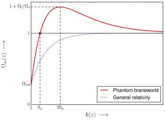
Figure 1: The red curve illustrates the dependence of the variable $\Omega_{m}$ on the dimensionless Hubble parameter $h=H/H_{0}$ on the phantom brane [see relation (14)]. The quantity $h$ is a monotonically growing function of redshift $z$, so that any value of $h$ can be related to the corresponding value of $z$ via (5). The red star indicates the position of the pole in the EOS of the effective dark energy at $h=h_{p}=\dfrac{\Omega_{\sigma}}{2\sqrt{\Omega_{\ell}}}$ which corresponds to $\Omega_{m}=1$. For comparison, we have also shown $\Omega_{m}$ as a function of $h$ in general relativity by the blue dotted curve.

The energy density and equation of state of the effective dark energy (7) in terms of the variable $\Omega_{m}$ can be expressed as

$$\frac{\rho_{\scriptscriptstyle E}}{3m^{2}} =H^{2}(1-\Omega_{m})\,,$$ (15)

$$w_{\scriptscriptstyle E} =-1-\left(\frac{1}{1+\ell H}\right)\frac{\Omega_{m}}{1-\Omega_{m}}\,.$$ (16)

Note that the point $\Omega_{m}(z_{p})=1$ represents a pole in the EOS of the effective dark energy. Dark energy is phantomlike ($w_{\scriptscriptstyle E}<-1$) in the region $\Omega_{m}(z)<1$, and quintessencelike ($w_{\scriptscriptstyle E}>-1$) when $\Omega_{m}(z)>1$.

III Evolution of the growth rate

The theory of cosmological perturbations on the brane is quite involved because of the presence of a large extra dimension. In particular, the bulk gravitational effects can lead to a nonlocal character of the resulting equations on the brane. Fortunately, the description of perturbations on sub-Hubble scales can be significantly simplified by using the quasistatic approximation KM which is based on the assumption of slow temporal evolution of the five-dimensional perturbations on sub-Hubble spatial scales. The validity of the quasistatic approximation for the phantom brane model was established in Viznyuk:2013ywa ; Bag:2016tvc .

Evolution of the matter density contrast $\delta_{m}=\delta\rho_{m}/\rho_{m}$ for the braneworld model in the quasistatic approximation is given by

$$\ddot{\delta}_{m}+2H\dot{\delta}_{m}=\frac{g_{\scriptscriptstyle E}\rho_{m}\delta_{m}}{2m^{2}}\,,$$ (17)

where $g_{\scriptscriptstyle E}$ is a time-dependent function that can be regarded as a renormalization factor for the gravitational constant. For the phantom brane, it is given by the relation

$${g}_{\scriptscriptstyle E}=1+\frac{1}{3\mu}$$ (18)

with

$$\mu=1+\ell H\left(1+\frac{\dot{H}}{3H^{2}}\right)=1+\frac{\ell H}{2}\Bigl{[}1-w_{\scriptscriptstyle E}(1-\Omega_{m})\Bigr{]}\,,$$ (19)

where $w_{\scriptscriptstyle E}$ is the effective equation of state of dark energy, given by (16).

We introduce the growth rate $f$ following Wang:1998gt :

$$f\equiv\frac{\differential\ln{\delta_{m}}}{\differential\ln{a}}\,.$$ (20)

Its evolution can easily be determined from (17):

$$\frac{\differential f}{\differential\ln{a}}+f^{2}+\left(2+\frac{\dot{H}}{H^{2}}\right)f=\frac{g_{\scriptscriptstyle E}\rho_{m}}{2m^{2}H^{2}}\,.$$ (21)

We are interested in the behavior of $f$ as a function of $\Omega_{m}$. In terms of the new variable $\Omega_{m}$, Eq. (21) becomes

$$6\,w_{\scriptscriptstyle E}\,\Omega_{m}(1-\Omega_{m})\frac{\differential f}{\differential\Omega_{m}}+2f^{2}+\left[1-3w_{\scriptscriptstyle E}(1-\Omega_{m})\right]f=3\,g_{\scriptscriptstyle E}\Omega_{m}\,,$$ (22)

where we have used the relation

$$\frac{\differential\,\Omega_{m}}{\differential\ln{a}}=3w_{\scriptscriptstyle E}\,\Omega_{m}(1-\Omega_{m})\,.$$ (23)

Braneworld-specific effects in (22) are encoded in the effective equation of state $w_{\scriptscriptstyle E}$. An additional modification, specific for the braneworld model, comes from the factor $g_{\scriptscriptstyle E}$, which renormalizes the gravitational constant for cosmological perturbations.

Note that the point $\Omega_{m}=1$, where the equation of state of the effective dark energy has a pole, is a regular point for the differential equation (22). So we do not expect any singularity in the behavior of $f$ at the moment of crossing the pole.

III.1 Series expansion in the asymptotic past

To find a solution of (22) in the $\Lambda$CDM model, one applies the method of series expansion around $\Omega_{m}=1$. In this case, the limit $\Omega_{m}\rightarrow 1$ is equivalent to $z\rightarrow\infty$, and the corresponding series expansion gives the best result for the values $z\gg 1$. Still, parametrizing the asymptotic solution as

$$f=\Omega_{m}^{\gamma}\,,$$ (24)

one finds that the growth index $\gamma$ varies very slowly with $\Omega_{m}$. Thus, solution (24) with $\gamma_{0}\approx 6/11$ describes the behavior of the growth rate with a sufficient accuracy in the whole range $z\geqslant 0$ Wang:1998gt ; Polarski:2016ieb .

We might expect a similar result for the braneworld model. However, repeating the general-relativistic analysis is impossible in this case because $\Omega_{m}$ is a nonmonotonic variable in the braneworld model. It crosses the value $\Omega_{m}=1$ when $z=z_{p}$, and then tends again to $\Omega_{m}=1$ as $z\rightarrow\infty$ (see Sec. II.2).

Consequently, if we wish to describe the behavior of the growth rate in the whole range $z\geqslant 0$, another variable should be chosen. Requiring this variable to be monotonic for $z\geqslant 0$, we choose it to be

$${x}\equiv\frac{1}{h(z)}\,,$$ (25)

where $h(z)$ is the dimensionless Hubble parameter (5). The specific feature of this new variable is that $x$ is a monotonically decreasing function of redshift $z$, with $x(0)=1$ and $x(z)\rightarrow 0$ as $z\to\infty$.

Our idea is to find the series expansion for $f(x)$ around $x=0$. We hope that, properly parametrizing the solution, we will be able to use this expansion to describe the behavior of the growth rate at the present epoch (corresponding to values of $x$ close to unity).

In terms of the variable $x$, we have

$$\frac{1}{\ell H}=\sqrt{\Omega_{\ell}}\,x\,,\qquad\Omega_{m}=1+2\sqrt{\Omega_{\ell}}\,{x}-\Omega_{\sigma}{x}^{2}\,.$$ (26)

The evolution of the growth rate is now given by

$$3x\Omega_{m}(x)\frac{\differential f}{\differential x}+2\left(1+\sqrt{\Omega_{\ell}}\,x\right)f^{2}+\left(1-2\sqrt{\Omega_{\ell}}\,x+3\Omega_{\sigma}x^{2}\right)f=3\left(1+\sqrt{\Omega_{\ell}}\,x\right)\Omega_{m}(x)\,g_{\scriptscriptstyle E}(x)\,,$$ (27)

where

$${g}_{\scriptscriptstyle E}=1+\frac{2\sqrt{\Omega_{\ell}}\,x(1+\sqrt{\Omega_{\ell}}\,x)}{3\left[(1+\sqrt{\Omega_{\ell}}\,x)^{2}+(\Omega_{\sigma}+\Omega_{\ell})x^{2}\right]}\,,$$ (28)

and $\Omega_{m}(x)$ is defined by (26).

In the following, we suppose that $x$ is sufficiently small so that both conditions

$$\Omega_{\sigma}x^{2}\ll 1~{}~{}\rm{and}~{}~{}\sqrt{\Omega_{\ell}}\,x\ll 1$$ (29)

are satisfied. We seek the solution of (27) in the form of a series expansion:

$$f\sim 1+f_{1}\Omega_{\sigma}x^{2}+f_{2}\Omega^{2}_{\sigma}x^{4}+f_{3}\sqrt{\Omega_{\ell}}\,x+f_{4}\Omega_{\ell}x^{2}+f_{5}\Omega_{\sigma}\sqrt{\Omega_{\ell}}\,x^{3}\,.$$ (30)

Performing the series expansions of (27) to the same order, we determine the coefficients:

$$f_{1}=-\,\frac{6}{11}\,,\quad f_{2}=-\,\frac{18\cdot 15}{17\cdot 11^{2}}\,,\quad f_{3}=\,\frac{11}{8}\,,\quad f_{4}=-\,\frac{153}{32\cdot 11}\,,\quad f_{5}=\frac{20}{77}\,.$$ (31)

This solves the problem of finding a series expansion for the growth rate in the asymptotic past, where $z\gg 1$ and $x\ll 1$. Now we study the possibility to parametrize the behavior of the growth rate in a way that extends this result to the broader range $x\leqslant 1$.

III.2 Parametrization of the growth rate in the asymptotic past

In analogy with the $\Lambda$CDM model, we expect that the perturbative expansion of the growth rate can be represented as the power of some expression with a slowly varying exponent. We will now try to find the correct parametrization of this form that fits the series expansion obtained in the previous section.

We consider the following ansatz for the growth rate:

$$f=\Omega_{m}^{\gamma}\Bigl{(}1+b\sqrt{\Omega_{\ell}}\,x\Bigr{)}^{\beta}\,,$$ (32)

with

$$\gamma=\gamma_{0}+\gamma_{1}(1-\Omega_{m})+\gamma_{2}\sqrt{\Omega_{\ell}}\,x\,,\qquad\beta=\beta_{0}+\beta_{1}\sqrt{\Omega_{\ell}}\,x\,.$$ (33)

This expression is a natural generalization of the $\Lambda$CDM parametrization $f=\Omega_{m}^{\gamma}$. The coefficient $\gamma_{2}$ here describes the correction of the general-relativistic growth index $\gamma$ due to brane effects. But, as we are about to show, modification of the growth index is not enough to describe the behavior of the growth rate in the braneworld model. Therefore, we introduce here the additional factor $\Bigl{(}1+b\sqrt{\Omega_{\ell}}\,x\Bigr{)}^{\beta}$, which becomes unity in the general-relativistic limit $\Omega_{\ell}\rightarrow 0$. The importance of this factor for the braneworld model is determined by the values of the coefficients $\beta_{0}$, $\beta_{1}$, and $b$, which will now be established.

Using (26), we perform a series expansion of (32), valid under conditions (29):

$$f\sim 1+\tilde{f}_{1}\Omega_{\sigma}x^{2}+\tilde{f}_{2}\Omega^{2}_{\sigma}x^{4}+\tilde{f}_{3}\sqrt{\Omega_{\ell}}\,x+\tilde{f}_{4}\Omega_{\ell}x^{2}+\tilde{f}_{5}\Omega_{\sigma}\sqrt{\Omega_{\ell}}\,x^{3}\,,$$ (34)

where

$$\tilde{f}_{1} =-\gamma_{0}\,,$$ (35)

$$\tilde{f}_{2} =\,\frac{\gamma_{0}(\gamma_{0}-1)}{2}-\gamma_{1}\,,$$ (36)

$$\tilde{f}_{3} =2\gamma_{0}+b\beta_{0}\,,$$ (37)

$$\tilde{f}_{4} =2\gamma_{2}-4\gamma_{1}+2\gamma_{0}(\gamma_{0}-1)+2b\beta_{0}\gamma_{0}+b\beta_{1}+\frac{b^{2}\beta_{0}(\beta_{0}-1)}{2}\,,$$ (38)

$$\tilde{f}_{5} =-\gamma_{2}+4\gamma_{1}-2\gamma_{0}(\gamma_{0}-1)-b\beta_{0}\gamma_{0}\,.$$ (39)

Now we compare these coefficients with the numerical values (31). Naturally, we start with the condition that the coefficients corresponding to linear terms coincide, namely, $\tilde{f}_{1}=f_{1}$ and $\tilde{f}_{3}=f_{3}$. This results in

$$\gamma_{0}=\frac{6}{11}\approx 0.54545\,,\qquad b\beta_{0}=\frac{25}{88}\approx 0.28409\,.$$ (40)

Now, from the conditions $\tilde{f}_{2}=f_{2}$ and $\tilde{f}_{5}=f_{5}$, we determine

$$\gamma_{1}\approx 0.00729\,,\qquad\gamma_{2}\approx 0.11034\,.$$ (41)

Finally, from $\tilde{f}_{4}=f_{4}$, we have

$$\beta_{1}\approx 0.142045-\frac{0.48057}{b}\,.$$ (42)

We see that $\beta_{1}$ can be made zero if we choose $b\approx 3.383$. In this case, we have

$$\beta_{0}\approx 0.084\,,\qquad\beta_{1}\approx 0\,.$$ (43)

So, finally, our parametrization is

$$f=\Omega_{m}^{\gamma}\Bigl{(}1+b\sqrt{\Omega_{\ell}}\,x\Bigr{)}^{\beta}\,,$$ (44)

with

$$\gamma\approx 0.54545+0.00729\,(1-\Omega_{m})+\alpha_{0}\sqrt{\Omega_{\ell}}\,x$$ (45)

and

$$\alpha_{0}\approx 0.11034\,,\qquad b\approx 3.383\,,\qquad\beta\approx 0.084\,.$$ (46)

The analytical parametrization of the growth rate given by (44)–(46) is expected to be valid at early times, when $\Omega_{m}$ is close to unity, hence $x$ is quite small. We have no reasons to believe that (44)–(46) will be valid for $x\sim 1$. Recall that $\Omega_{m}$ is not a monotonic function, and this fact may result in a different parametrization for $x\sim 1$.

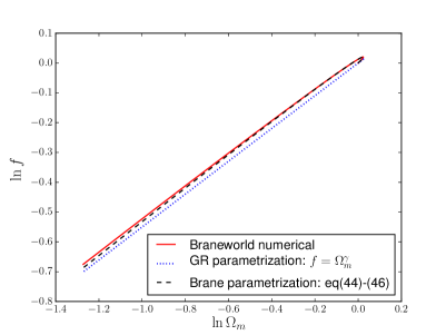
(a) $\Omega_{\ell}=0.025$

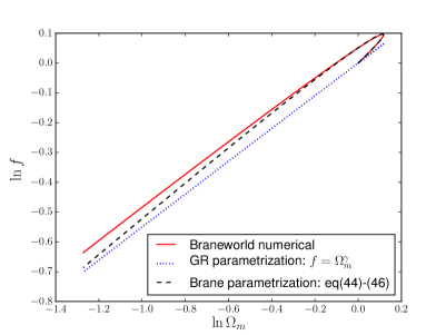
(b) $\Omega_{\ell}=0.2$

Figure 2: The analytical expression for $f$ given in (44)–(46) (shown by the dashed black curves), is compared with the numerical solution for the growth rate (red line) for two values of the brane parameter $\Omega_{\ell}$. For comparison, we also present here the parametrization $f=\Omega_{m}^{\gamma}$ (blue dotted curves) with the general-relativistic parameter $\gamma$ given by (45) with $\Omega_{\ell}=0$. The curves start from the matter domination, characterized by $\Omega_{m}=1=f$ and end at the present epoch when $\Omega_{m}=\Omega_{m0}$. We assume $\Omega_{m0}=0.28$ for illustration purposes. As is expected, the analytical solution (44)–(46) is very accurate at early times. At late times, solution (44)–(46) starts to deviate from the numerical solution as $\Omega_{m}$ becomes significantly lower than unity. As we increase $\Omega_{\ell}$, this deviation becomes more profound at the present epoch. Note that the numerical curve is multivalued for $\Omega_{m}\geqslant 1$. For $\Omega_{\ell}=0.2$, this corresponds to $z\gtrsim 1.27$. For $\Omega_{\ell}=0.025$, the growth rate becomes multivalued for $z\gtrsim 2.27$.

Let us compare the analytical expression (44)–(46) with the solution for $f$ obtained by the numerical integration of (22) (see Fig. 2). As expected, (44)–(46) accurately matches the numerical solution at early times and becomes inaccurate at late times, when $\Omega_{m}$ falls significantly below unity. We also note that, as we increase $\Omega_{\ell}$, the analytical expression starts to deviate from the exact solution at higher values of $\Omega_{m}$ (i.e., at earlier time) and the deviation at the present epoch is larger.

For comparison, we also plot in Fig. 2 the general-relativistic (GR) parametrization, $f=\Omega_{m}^{\gamma}$. It is evident from this illustration that the GR parametrization fails to describe the behavior of the growth rate in the braneworld model. In fact, the exact (numerical) solution for the growth rate is multivalued in the range $\Omega_{m}\geqslant 1$ , $h\geqslant h_{p}$ (see Fig. 1). Therefore, the growth rate on the phantom brane cannot in principle be described by the GR parametrization, $f=\Omega_{m}^{\gamma}$, which is single-valued for all $\Omega_{m}$. To correctly describe the exact solution of $f$ at all times, we need to introduce an extra factor, such as the one in (44).

To get closer to the parametrization valid for all times, we also need to study the future asymptote for the growth rate. This is done in the next subsection.

III.3 Future asymptotics

Here, we try to obtain the solution for $f$ in the distant future when $\Omega_{m}\to 0$ (or $z\to-1$). In both GR and the phantom braneworld, $w_{E}\to-1$ in the distant future. Using a simple trial solution

$$f=C\,\Omega_{m}^{\gamma}\;,$$ (47)

one can find from (22) that $\gamma=2/3$ in both general relativity and the braneworld model, by neglecting terms proportional to $f^{2}$ and $\Omega_{m}$. Indeed, in the limit $\Omega_{m}\to 0$, one can neglect $\Omega_{m}^{2\gamma}$ and $\Omega_{m}$ with respect to $\Omega_{m}^{\gamma}$ assuming $\gamma<1$ in advance.

The constant $C$ in (47) can be determined from the numerical integration of (22). In general relativity, we get

$$f_{\rm GR}\approx C_{\rm GR}\,\Omega_{m}^{2/3}\quad\text{in the limit}\quad\Omega_{m}\rightarrow 0\,,$$ (48)

where the constant $C_{\rm GR}\approx 1.73$ is quite robust under variation of the parameter $\Omega_{m0}$. The behavior of the growth rate in the asymptotic future in general relativity is illustrated in Fig. 3.

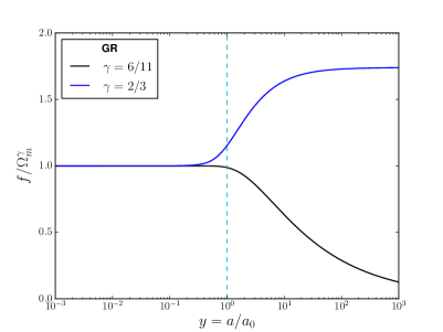
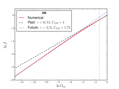
Figure 3: Both panels show that, in general relativity (GR), $f$ has two distinct solutions in the two asymptotics — in the past and in the future. Both solutions are parametrized by $f=C\,\Omega_{m}^{\gamma}$ with different values of the parameter $\gamma$ and the constant $C$. The dashed vertical cyan lines represent the present epoch. In the left panel, $f$ is calculated numerically and is represented by the red curve in the right panel. The blue curve in the left panel is flat in the distant future, i.e., for $a/a_{0}\gg 1$. This reveals that, in the future asymptotics, $f\propto\Omega_{m}^{2/3}$ where the proportionality constant is estimated as $C_{\rm GR}\approx 1.73$. On the other hand, deep in the matter domination, $\Omega_{m}\to 1$ and $f\to 1$. Therefore, both the black and blue curves in the left panel approach unity when $a/a_{0}\ll 1$. In the right panel, we compare the two asymptotic solutions for $f$ with the numerical solution. The past asymptotic solution, $f\approx\Omega_{m}^{6/11}$, is reasonably valid near the present epoch in GR, as is evident from both panels.

For the phantom braneworld model, we found the following asymptotic solution:

$$f_{\rm BW}=C_{\rm BW}\,\Omega_{m}^{2/3}\quad\text{in the limit}\quad\Omega_{m}\rightarrow 0\,.$$ (49)

Numerical analysis reveals that the constant $C_{\rm BW}$ here can be related to the general-relativistic value $C_{\rm GR}$ as follows:

$$\frac{C_{\rm BW}}{(1+b\sqrt{\Omega_{\ell}}x)^{\beta}}\approx 1.73=C_{\rm GR}\;,$$ (50)

which is valid for a huge range of $\Omega_{\ell}$. Note that $h=1/x\approx(\sqrt{\Omega_{\sigma}+\Omega_{\ell}}-\sqrt{\Omega_{\ell}})$ is almost constant in the limit $\Omega_{m}\to 0$.

Thus one can conclude that, in the future asymptotics on the phantom brane, we have

$$f=C_{\rm GR}\,\Omega_{m}^{\gamma}(1+b\sqrt{\Omega_{\ell}}x)^{\beta}\,,$$ (51)

where $C_{\rm GR}\approx 1.73$, $\gamma\approx 2/3$, and $\beta$ and $b$ are the same as in (46) and (54): $\beta=0.084$, $b=3.383$. Therefore, in both the past and future asymptotics, the growth rate on the phantom brane behaves as

$$f_{\rm BW}\approx f_{\rm GR}\times(1+b\sqrt{\Omega_{\ell}}x)^{\beta}\,.$$ (52)

The deviation of the past asymptotic analytical solution for $f$, given in (44)–(46), from the exact solution near the present epoch can be attributed to the smooth transition from the past asymptotic solution to the future one. Even in GR, we notice that $f$ behaves entirely different in the two asymptotics — in the past and in the future. It is impossible to obtain a single expression for $f$ in terms of $\Omega_{m}$ which would be valid in the entire range of evolution, even in GR. Fortunately, in GR, the past asymptotic solution does not deviate much from the exact one near the present epoch, and one can compensate for this small deviation by adding higher-order correction terms to $\gamma$. Nevertheless, as we have seen in the previous subsection, adding higher-order correction terms to $\gamma$ on phantom braneworld does not significantly improve the accuracy of parametrization (44)–(46) at late times.

Remarkably, the growth rate on the phantom brane acquires the same additional multiplicative factor $(1+b\sqrt{\Omega_{\ell}}x)^{\beta}$ to its GR counterpart in both the past and the future asymptotics. So we can expect that the parametrization

$$f=\Omega_{m}^{\gamma}(1+b\sqrt{\Omega_{\ell}}x)^{\beta}\,.$$ (53)

will be reasonably valid at all times (past–present–future). This assumption will be confirmed by the numerical simulations described in the next section.

IV Universal parametrization of the growth rate

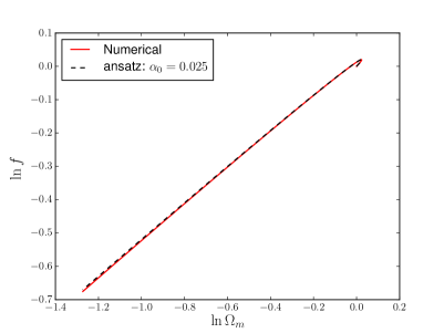
(a) $\Omega_{\ell}=0.025$

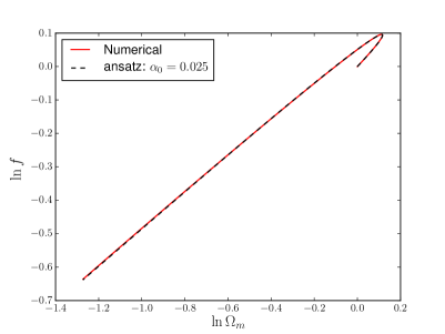
(b) $\Omega_{\ell}=0.2$

Figure 4: Ansatz (54)–(55) (dashed black curves) is compared with the numerical solution (red curves) for two values of the brane parameter $\Omega_{\ell}$, starting from the matter domination until the present epoch. We find that the ansatz is quite accurate for braneworld effects as strong as $\Omega_{\ell}=2.0$.

As we demonstrated in the previous section, the growth rate $f$ for the phantom brane model behaves differently at different asymptotics. Parametrization (44)–(46) works well in the asymptotic past, but fails to fit a numerical solution at the present epoch. Therefore, in this section we seek for an ansatz that describes the evolution of $f$ reasonably well in the past, at least till the present epoch.

We have tried to get better fit with the numerical result by changing the values of the parameters in (44)–(46). In this way, we were able to find the ansatz that gives excellent match to the numerical solutions till the present epoch. The ansatz is given by

Figure 5: Percentage error of the ansatz (54)–(55) is shown for different values of the brane parameter $\Omega_{\ell}$, starting from the matter domination until the present epoch. Here, $f_{nu}$ and $f_{an}$ represent the numerical solution for $f$ and the ansatz (54) respectively. Note that, during matter domination $\Omega_{m}\to 1$ and, at the present epoch, $\Omega_{m}=\Omega_{m0}=0.28$.

$$f=\Omega_{m}^{\gamma}\Bigl{(}1+b\sqrt{\Omega_{\ell}}\,x\Bigr{)}^{\beta}=\Omega_{m}^{\gamma}\left(1+\frac{b}{\ell H}\right)^{\beta}\;,$$ (54)

with

$$\gamma\approx 6/11+0.00729\,(1-\Omega_{m})+\frac{\alpha_{0}}{\ell H}\;,\quad\text{where}\quad\alpha_{0}=0.025\;,$$ (55)

and $\beta$, $b$ are same as in (46), i.e., $\beta=0.084$, $b=3.383$.

Ansatz (54)–(55) differs from (44)–(46), obtained by considering the past asymptotics, by the value of a single parameter $\alpha_{0}$ (recall that $\alpha_{0}\approx 0.11$ in the exact asymptotic solution for $x\equiv 1/h\ll 1$). Figure 4 shows the comparison of ansatz (54)–(55) with the exact solution. We see that the exact solution of $f$ is reasonably well described by the ansatz at least till the present epoch $z\gtrsim 0$, even for braneworld effects as strong as $\Omega_{\ell}=0.2$. The error of this ansatz is of the order $0.1\%$ for values of $\Omega_{\ell}$ consistent with the observations. The evolution of the error for different values of $\Omega_{\ell}$ is shown in Fig. 5. As we can see, ansatz (54)–(55) is reasonably valid till the present epoch for a wide range of $\Omega_{\ell}$. For example, the maximum error is below $1\%$ even for the brane parameter as large as $\Omega_{\ell}=0.5$.

For comparison, we can estimate the maximal error for the standard general-relativistic parametrization $f=\Omega_{m}^{\gamma}$ from Fig. 2. We note that the parametrization $f=\Omega_{m}^{\gamma}$ results in $f=1$ whenever $\Omega_{m}=1$ for any $\gamma$. On the other hand, the exact solution for $f$ on the phantom brane reveals that $f>1$ at $z=z_{p}$ (the pole in the EOS) when $\Omega_{m}=1$. The discrepancy of the parametrization $f=\Omega_{m}^{\gamma}$ with the numerical solution at this point is about $0.052$ for $\Omega_{\ell}=0.2$, and $0.013$ for $\Omega_{\ell}=0.025$. Consequently, the maximal error of the parametrization $f=\Omega_{m}^{\gamma}$ with any $\gamma(z)$ cannot be smaller than $5.2\%$ for $\Omega_{\ell}=0.2$, and $1.3\%$ for $\Omega_{\ell}=0.025$. For instance, the maximal errors of the parametrization with the general-relativistic $\gamma(z)$ in these cases constitute $6.4\%$ and $2.7\%$, respectively.

V Conclusions

Our analysis demonstrates that the growth rate for the phantom brane model can be parametrized as

$$f=\Omega_{m}^{\gamma}\left(1+\frac{b}{\ell H}\right)^{\beta}\,,$$ (56)

with the growth index $\gamma$ and other parameters given in (54)–(55). Such a form of the growth rate provides an excellent fit to numerical simulations from very large $z$ to the present epoch. We have established that the above parametrization is highly accurate (the maximum error is of the order $0.1\%$) for a wide range of the brane parameter $\Omega_{\ell}$.

The standard general-relativistic parametrization $f=\Omega_{m}^{\gamma}$ fails to describe the behavior of the growth rate on the phantom brane because the exact solution for the growth rate in this case is multivalued in the domain $\Omega_{m}\geqslant 1$, whereas the function $f=\Omega_{m}^{\gamma}$, is single-valued for all $\Omega_{m}$, and moderate dependence of $\gamma$ on redshift cannot remedy the situation. For example, the exact solution is multivalued for $z\gtrsim 1.27$ if $\Omega_{\ell}=0.2$, or for $z\gtrsim 2.27$ if $\Omega_{\ell}=0.025$. The maximal error of the parametrization $f=\Omega_{m}^{\gamma}$ with any $\gamma(z)$ cannot be smaller than $5.2\%$ for $\Omega_{\ell}=0.2$, and $1.3\%$ for $\Omega_{\ell}=0.025$. In the case of general-relativistic $\gamma(z)$, these errors are as large as $6.4\%$ and $2.7\%$, respectively.

A similar situation can be expected for other models of modified gravity. Our results therefore suggest that a general parametrization of the form

$$f=K(a)\Omega_{m}^{\gamma}(a)$$ (57)

may be more suitable for the description of perturbations in modified gravity models than the usual approach based on $f=\Omega_{m}^{\gamma}(a)$.

References

- (1) R. Maartens and K. Koyama, Brane-world gravity, Living Rev. Relativ. 13, 5 (2010) [arXiv:1004.3962].
- (2) B. Novosyadlyj, V. Pelykh, Y. Shtanov and A. Zhuk, Dark energy: Observational evidence and theoretical models, arXiv:1502.04177.
- (3) H. Collins and B. Holdom, Brane cosmologies without orbifolds, Phys. Rev. D 62, 105009 (2000) [hep-ph/0003173].
- (4) G. Dvali, G. Gabadadze and M. Porrati, 4D gravity on a brane in 5D Minkowski space, Phys. Lett. B 485, 208 (2000) [hep-th/0005016]; G. Dvali and G. Gabadadze, Gravity on a brane in infinite-volume extra space, Phys. Rev. D 63, 065007 (2001) [hep-th/0008054].
- (5) Yu. V. Shtanov, On brane world cosmology, hep-th/0005193.
- (6) C. Deffayet, Cosmology on a brane in Minkowski bulk, Phys. Lett. B 502, 199 (2001) [hep-th/0010186].
- (7) C. Deffayet, G. R. Dvali and G. Gabadadze, Accelerated universe from gravity leaking to extra dimensions, Phys. Rev. D 65, 044023 (2002) [astro-ph/0105068].
- (8) C. Charmousis, R. Gregory, N. Kaloper and A. Padilla, DGP specteroscopy, J. High Energy Phys. 10 (2006) 066 [hep-th/0604086]; D. Gorbunov, K. Koyama and S. Sibiryakov, More on ghosts in the Dvali–Gabadaze–Porrati model, Phys. Rev. D 73, 044016 (2006) [hep-th/0512097]; K. Koyama, Ghosts in the self-accelerating universe, Classical Quantum Gravity 24, R231 (2007) [arXiv:0709.2399].
- (9) V. Sahni and Yu. Shtanov, Brane world models of dark energy, J. Cosmol. Astropart. Phys. 11 (2003) 014 [astro-ph/0202346].
- (10) U. Alam and V. Sahni, Confronting braneworld cosmology with supernova data and baryon oscillations, Phys. Rev. D 73, 084024 (2006) [astro-ph/0511473].
- (11) A. Lue and G. D. Starkman, How a brane cosmological constant can trick us into thinking that , Phys. Rev. D 70, 101501 (2004) [astro-ph/0408246]
- (12) R. Lazkoz, R. Maartens and E. Majerotto, Observational constraints on phantom-like braneworld cosmologies, Phys. Rev. D 74, 083510 (2006) [astro-ph/0605701].
- (13) U. Alam, S. Bag and V. Sahni, Constraining the cosmology of the phantom brane using distance measures, Phys. Rev. D 95, 023524 (2017) [arXiv:1605.04707].
- (14) S. Bag, A. Viznyuk, Y. Shtanov and V. Sahni, Cosmological perturbations on the phantom brane, J. Cosmol. Astropart. Phys. 07 (2016) 038 [arXiv:1603.01277].
- (15) U. Alam and V. Sahni, Confronting braneworld cosmology with supernova data and baryon oscillations, Phys. Rev. D 73, 084024 (2006) [astro-ph/0511473].
- (16) L. Lombriser, W. Hu, W. Fang and U. Seljak, Cosmological constraints on DGP braneworld gravity with brane tension, Phys. Rev. D 80, 063536 (2009) [arXiv:0905.1112].
- (17) L. Xu, Confronting DGP braneworld gravity with cosmico observations after Planck data, J. Cosmol. Astropart. Phys. 02 (2014) 048 [arXiv:1312.4679].
- (18) S. Bhattacharya and S.R. Kousvos, Constraining the phantom braneworld model from cosmic structure sizes, Phys. Rev. D 96, 104006 (2017). [arXiv:1706.06268]
- (19) T. Delubac, et al., Baryon acoustic oscillations in the Ly forest of BOSS DR11 quasars, Astron. Astrophys. 574, A59 (2015) [arXiv:1404.1801]; J. E. Bautista, et al., Measurement of baryon acoustic oscillation correlations at with SDSS DR12 Ly-Forests, Astron. Astrophys. 603, A12 (2017) [arXiv:1702.00176]; G.-B. Zhao, et al., The clustering of the SDSS-IV extended Baryon Oscillation Spectroscopic Survey DR14 quasar sample: a tomographic measurement of cosmic structure growth and expansion rate based on optimal redshift weights, arXiv:1801.03043.
- (20) V. Sahni, A. Shafieloo and A.A. Starobinsky, Model independent evidence for dark energy evolution from Baryon Acoustic Oscillations, Astrophys. J. 793, L40 (2014) [arXiv:1406.2209].
- (21) A. Shafieloo, B. L’Huiller and A.A. Starobinsky, Falsifying CDM: Model-Independent Tests of the Concordance Model with eBOSS DR14Q and Pantheon, arXiv:1804.04320 [Phys. Rev. Lett. (to be published)].
- (22) P. J. E. Peebles, The Large-Scale Structure of the Universe (Princeton University Press, Princeton, New Jersey, 1980).
- (23) L. M. Wang and P. J. Steinhardt, Cluster abundance constraints on quintessence models, Astrophys. J. 508, 483 (1998) [astro-ph/9804015].
- (24) D. Polarski, A. A. Starobinsky and H. Giacomini, When is the growth index constant?, J. Cosmol. Astropart. Phys. 12 (2016) 037 [arXiv:1610.00363].
- (25) E. V. Linder and R. N. Cahn, Parameterized beyond-Einstein growth, Astropart. Phys. 28, 481 (2007) [astro-ph/0701317].
- (26) H. Wei, Growth index of DGP model and current growth rate data, Phys. Lett. B 664, 1 (2008) [arXiv:0802.4122].
- (27) Y. Gong, The growth factor parameterization and modified gravity, Phys. Rev. D 78, 123010 (2008) [arXiv:0808.1316].
- (28) V. Q. Phong, Dynamic of the accelerated expansion of the universe in the DGP model, Communications in Physics 21, 03 (2011) [arXiv:1207.2365].
- (29) M. Ishak and J. Dossett, Contiguous redshift parameterizations of the growth index, Phys. Rev. D 80, 043004 (2009) [arXiv:0905.2470].
- (30) S. Chen and J. Jing, Improved parametrization of the growth index for dark energy and DGP models, Phys. Lett. B 685, 185 (2010) [arXiv:0908.4379].
- (31) M. A. Resco and A. L. Maroto, Parametrizing growth in dark energy and modified gravity models, Phys. Rev. D 97, 043518 (2018) [arXiv:1707.08964].
- (32) V. Sahni and A.A. Starobinsky, Reconstructing Dark Energy, Int. J. Mod. Phys. D15, 2105 (2006) [astro-ph/0610026].
- (33) K. Koyama and R. Maartens, Structure formation in the DGP cosmological model, J. Cosmol. Astropart. Phys. 01 (2006) 016 [astro-ph/0511634].
- (34) A. Viznyuk, Y. Shtanov and V. Sahni, A no-boundary proposal for braneworld perturbations, Phys. Rev. D 89, 083523 (2014) [arXiv:1310.8048].