The reported durations of GOES Soft X-Ray flares in different solar cycles

Abstract

The Geostationary Orbital Environmental Satellites (GOES) Soft X-ray (SXR) sensors have provided data relating to, inter alia, the time, intensity and duration of solar flares since the 1970s. The GOES SXR Flare List has become the standard reference catalogue for solar flares and is widely used in solar physics research and space weather. We report here that in the current version of the list there are significant differences between the mean duration of flares which occurred before May 1997 and the mean duration of flares thereafter. Our analysis shows that the reported flare timings for the pre-May 1997 data were not based on the same criteria as is currently the case.

This finding has serious implications for all those who used flare duration (or fluence, which depends on the chosen start and end times) as part of their analysis of pre-May 1997 solar events, or statistical analyses of large samples of flares, e.g. as part of the assessment of a Solar Energetic Particle forecasting algorithm.

1 Introduction

Solar flares are sudden brightenings across the whole of the electromagnetic spectrum, typically from a small spatial region in the Sun’s corona. They have been known to occur since the middle of the 19th century (Carrington (1859); Hodgson (1859)). Since 1976 they have been classified according to their peak emissions in the 1 - 8 Å band of the X-ray Sensors (XRS) Garcia (1994)) carried by a series of Geostationary Orbital Environmental Satellites (GOES). X-class flares have a peak soft X-ray (SXR) emission of 10^-4 W/m² or higher; M-class flares a peak SXR emission between 10^-5 and 10^-4 W/m²; C, B, and A-class flares are similarly defined (Cliver (2000)).

Flare duration has been an important parameter for those involved in the field of solar physics for decades. For many years flares have been grouped into two types: “gradual” or “long duration”, and “impulsive”. Gradual flares remain within 10% of their peak intensity for more than 1 hour, whereas impulsive flares return to below that threshold within 1 hour (e.g. Cane et al. (1986); Kallenrode et al. (1992)). This classification has formed the basis of a large body of work.

Furthermore, flare duration and fluence have been known to be a significant parameter in relation to the production of Solar Energetic Particles (SEPs) within a space weather forecasting environment, as will be shown in Section 3. Evaluation of SEP forecasting algorithms over long time ranges requires a consistent flare duration dataset.

Since 1976 the GOES SXR Flare List has become the standard solar flare catalogue. The list may be accessed through a number of different sources: e.g. directly from NOAA’s National Centers for Environmental Information website, through the Heliophysics Integrated Observatory (“Helio”) website (Aboudarham et al. (2012)), and by using routines in both SolarSoft SSWIDL (Freeland and Handy (1998)) and SunPy (The SunPy Community et al. (2015)). In SolarSoft the list is retrieved by calling the routine “get_gev” with a specified start and end time. In SunPy the relevant routine is “sunpy.instr.goes.get_goes_event_list”. Relevant URLs for Helio, SolarSoft, and SunPy are given in the Acknowledgements Section.

A significant difference in the reported mean duration of X-class flares between a time range incorporating Solar Cycles 21 and 22, and one incorporating Cycles 23 and 24 was noted by Swalwell et al. (2017). Those authors did not seek to explain the discrepancy.

In this work differences between mean flare duration as reported by the GOES SXR Flare List in different solar cycles are analysed. Flare data are now available for four full solar cycles. The GOES SXR Flare List which is used in our analysis below was obtained from the Helio website (Aboudarham et al. (2012)), but these results have been independently confirmed using other files on the National Geophysical Data Center website.

2 Data Analysis

The start time of a GOES SXR flare, as currently defined by NOAA, is the time when 4 consecutive values in the 1-minute 1-8 Å data meet all 3 of the following conditions:

• All 4 values are above the B1 threshold

• All 4 values are strictly increasing

• The last value is greater than 1.4 times the value which occurred 3 minutes earlier

The peak time of the flare is when the SXR flux reaches its maximum (and it is the value of the SXR flux at this time which defines the class of the flare). The flare end time is defined as the time when the flux reading returns to 1/2 the ’peak’, where the peak is the flux at maximum minus the flux value at the start of the event. Here we take flare duration to be the total time between the reported flare start time and flare end time; “rise time” is the time between flare start time and the time of flare maximum; and “decay time” is the time between the time of flare maximum and the flare end time. At the time of writing, events with fast rise times are derived automatically by an algorithm processing the SXR data, whereas those with slow rise times are recorded manually.

Figure 1 is a bar plot showing the mean duration (in minutes) of flares of different classes in each of the last 4 solar cycles derived from the GOES SXR Flare List: in this work Solar Cycle 21 is taken to have started on 1 January 1976, Cycle 22 on 1 January 1986, Cycle 23 on 1 January 1996, and Cycle 24 on 1 January 2008. From left to right the bars represent B-class flares, then C-class, M-class, and X-class. It is readily apparent that the mean reported duration of both M and X-class flares in Solar Cycles 21 and 22 is much longer than in Cycles 23 and 24.

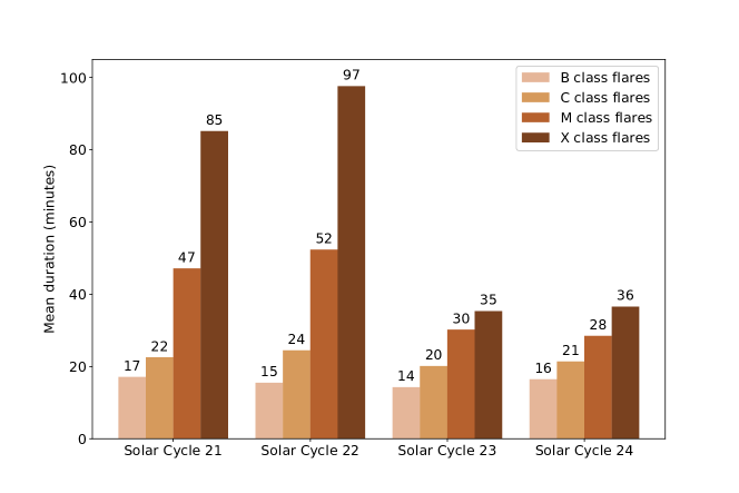
Figure 1: Mean reported duration (in minutes) of flares of different classes in each of the last 4 solar cycles as derived from the GOES SXR list. From left to right bars represent B-class flares, then C-class, M-class, and X-class.

As the difference in mean duration is most apparent for flares of a higher class, we concentrate on X-class flares. We plotted the 1-minute time-averaged SXR data for each reported X-class flare from 1 January 1986 onwards (as the NOAA website does not publish such data for earlier periods). Table 1 shows the reported timings of a representative sample of 4 X-class flares in the GOES SXR List which occurred in Solar Cycle 22. Column 1 gives the flare class, column 2 the date of the event, and columns 3, 4, and 5 the reported start time, peak time, and end time of each flare.

Table 1: The reported timings of a sample of 4 X-class flares which occurred during Solar Cycle 22. Column 1 gives the flare class, column 2 the date of the event, and columns 3, 4, and 5 the reported start time, peak time, and end time of each flare.

Flare class	Date	Reported start	Reported peak	Reported end
X1.6	1988-06-23	08:56	09:27	10:03
X2.4	1988-06-24	16:03	16:48	16:54
X1.1	1989-01-07	04:12	04:36	04:44
X2.3	1989-01-13	08:29	10:18	10:45

Figure 2 shows plots of the 1-minute time-averaged SXR downloaded from the NOAA website for each of this sample of 4 flares. Time is plotted on the x-axis: the starting point for each plot was 2 hours prior to the reported start time of the flare, and the end point was 6 hours after its reported end. On the y-axis is plotted the 1-8 Å 1-minute time-averaged SXR flux in W/m².

On each plot a light-blue vertical line is drawn at the flare’s start time as reported in the catalogue; a vertical green line at its reported peak; and a vertical purple line at its reported end. The horizontal dotted brown line is drawn at half the peak of the SXR flux as previously defined(which represents the end of the flare according to the NOAA criteria). The name of the GOES spacecraft carrying the SXR sensor is specified at the top of each plot, as is the reported start time of the flare and its reported class.

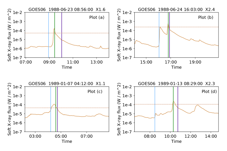
Figure 2: Soft X-ray flux for a sample of 4 X-class flares in Solar Cycle 22. Time is shown on the x-axis, and the 1-minute time-averaged soft X-ray flux in W/m² on the y-axis. On each plot the vertical light-blue line is drawn at the flare’s reported start time; a vertical green line at its reported peak; and a vertical purple line at its reported end. The horizontal dotted brown line is drawn at half the peak of the SXR flux (as defined by NOAA).

For the flare shown in plot (a) it can be seen that the reported start time is several minutes earlier than the actual start of the rise in SXR flux; the reported peak is slightly different from the actual peak; and the reported end of the flare is many minutes later than it ought to be according to the NOAA definition. Plot (b) shows the SXR flux of an X2.4 flare which occurred the day after the flare shown in plot (a). Here, there were 2 X-class flares in quick succession, but only 1 is reported, and the times of the 2 flares have been combined - the reported start of the flare is for the first of the 2 events, but the reported peak and end are for the second flare. For the flare shown in plot (c) reported start and end times are slightly awry, and the reported peak is some time later than the peak in SXR flux; and in plot (d) both reported start and end times do not appear to accord with the NOAA definition.

To illustrate that the qualitative behaviour seen in Figure 2 is ubiquitous, we considered flares of class $\geq$ M5 and developed a method of calculating rise and decay times directly from the SXR flux time series. To obtain the flare start time we took the time of the peak as originally reported and looked back to find the time when the SXR flux was either 5% of the peak flux, or where the slope (i.e. the derivative) of a highly smoothed long-channel light curve reached 5% of the peak slope, whichever time was the later. The value of 5% was chosen so as to exclude pre-flare heating, and to ensure that if there had been another peak prior to the flare of interest the start time would fall between the two flares. To find the flare end time we looked forward from the originally reported peak time to find the time where the SXR flux fell to 50% of the peak value. Whilst the method was surprisingly accurate in finding flare start time, in a small number of cases the timing of the start of the flare was adjusted manually based upon inspection of the data.

Figure 3 compares flare rise times as a fraction of total flare duration for flares greater than class M5 between 1986 and 2015. The ratio of rise time to duration appears on the y-axis, and flare sequence number on the x-axis. The top plot of Figure 3 shows the original timings as reported in the GOES SXR Flare List: the ratio is centred around 0.19 (median) for flares which occurred prior to 1997, but the ratio changes to be centred around 0.58 (median) after 1997. The bottom plot of the same Figure shows the same ratio but in this case based upon our timings, and for both pre and post 1997 flares the ratio remains centred at a median value of 0.50.

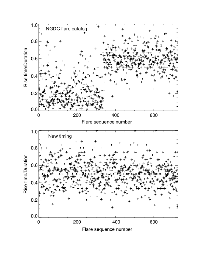
Figure 3: Plots of the ratio of flare rise time to total flare duration for flares of class $\geq$ M5 between 1986 and 2015. In the top plot the ratio is derived using timings from the GOES SXR Flare List, whereas the ratio for the bottom plot is derived from our timings.

It is clear from Figure 3 that a significant change occurred in 1997. With a view to discovering when in 1997 this happened, we examined plots similar to those shown in Figure 2 for the more frequent M-class flares. It is apparent that the reported flare timings up to and including the M1.9 flare on 1 April 1997 do not accord with the NOAA definition, whereas the timings of the next M-class flare (which was an M1.3 flare on 21 May 1997) do accord with that definition. The change in the way that flare timings are reported occurred within that nearly two month period.

We also considered the distribution of flare duration shown in Figure 4 considering M and X-class flares only. The distribution for the period prior to May 1997 (brown line) is compared with that post May 1997 (purple line). It is readily apparent that there was a greater proportion of large flares which were reported to have a duration of less than about 30 minutes post May 1997. Conversely there was a greater proportion of large flares reported to last longer than about 30 minutes prior to May 1997.

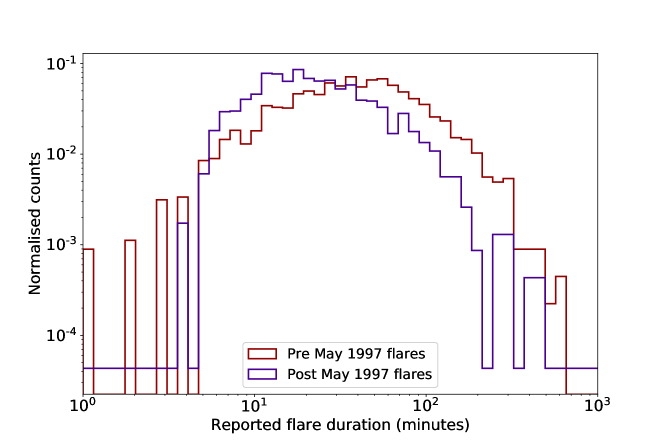
Figure 4: Distribution of reported flare durations for M and X-class flares in the GOES SXR Flare List for the time range prior to May 1997 (brown line) and after May 1997 (purple line). Flare counts are normalised to the overall number of flares in each time range.

3 Discussion

Our analysis of the GOES SXR Flare List shows that there are clear systematic differences in mean flare duration between a time range including Solar Cycles 21 and 22, and one including Solar Cycles 23 and 24. The effect is particularly clear for X and M-class flares: the mean duration of X-class flares in Cycles 21 and 22 was respectively 2.4 and 2.7 times as long as that for Cycle 23; for M-class flares the mean duration for Cycles 21 and 22 was respectively 1.6 and 1.7 times as long as that for Cycle 23.

Veronig et al. (2002) reported that prior to 1997 the reported SXR flare times were taken from the associated H$\alpha$ event. These timings were originally reported in the Solar-Geophysical Data Reports (commonly called the “Yellow Books”) and which are now mostly available online. The table headed “GOES Solar X-ray Flares” in those books often has an “Editor’s Note” at the bottom which reads “Please note that whenever optical flares are given, the times given are times of the optical flares and not the times of the X-ray flares”. Our analysis indicates that this is the case for most, especially large, flares but we have not checked all the data manually. This information, however, is not propagated within the tools such as Helio, SolarSoft, or Sunpy.

H$\alpha$ flare duration is defined visually, i.e. how long the flare can be seen, and the timings given in the Yellow Books are based upon reports from many different observing stations. It is therefore entirely unsurprising that these times do not in general correspond with the definition of flare timings published by NOAA. It seems, therefore, that the differences reported here stem from a change of use of H$\alpha$ timings to timings based upon SXR flux as measured by the GOES X-ray Sensors. Whatever the cause, pre May 1997 flare timings are not directly comparable with post May 1997 flare timings.

This finding can have serious implications for some statistical studies that used the GOES X-ray flare listings prior to May 1997. However, we have to be careful to distinguish those works that used the flare listings for only the correct peak X-ray fluxes (e.g. Garcia (2004); Belov (2009)) and not for times or fluences. Further, many authors used the pre-1998 GOES XRS flux-time profiles to determine independently their own flare times and fluences (e.g. Cane et al. (1986); Balch (2008); Laurenza et al. (2009); Ji et al. (2014); Trottet et al. (2015); Papaioannou et al. (2016)) or used those independent lists for further analyses (e.g. Kahler and Ling (2015); Kahler et al. (2015)). Finally, there have been many SEP event studies based on X-ray flare reports together with Coronal Mass Ejections (CMEs) from the SOHO/LASCO catalog listings (e.g. Miteva et al. (2013); Park and Moon (2014); Dierckxsens et al. (2015); Belov (2017)). Those CME listings began in January 1996, so there is an overlap of CME reports and GOES SXR flare listings from that time to May 1997. During that period of low solar activity there were only seven $>$M1 flares, two $>$M3 flares, and no NOAA $>$10 pfu at $>$10 MeV SEP events. The impact of the incorrect flare listings on those SEP studies and on flare-CME comparisons (e.g. Yashiro and Gopalswamy (2009)) should therefore be minimal.

We know of significant impacts to two (involving current authors) recent reports on SEP events. In their validation of the Proton Prediction System (PPS) Kahler et al. (2017) calculated X-ray flare fluences from 1986 to 2014 as the product of the flare rise times (onset to peak) and the peak fluxes obtained from the NOAA listings. Of their 716 $>$M5 X-ray flare candidates, 344 were before May 1997, as were 26 of their 67 SEP events. The incorrectly reported flare rise times in the listings before May 1997 (shown in the top panel of Figure 3) would suggest that Kahler et al. (2017) used inaccurate X-ray fluences, which would have affected the forecasting of SEP events with PPS for that time. The PPS validation with three groups of 8800 MHz bursts in their work was independent of the X-ray fluences and remains valid.

In the second impacted report Swalwell et al. (2017) defined two algorithms to forecast $>$40 MeV SEP events. Their second algorithm using X-class flares to forecast SEP events was tested over two time ranges: 1996 to 2013 and 1980 to 2013. While that algorithm was based only on flare intensities, they also displayed the flare durations in their Figure 11, which shows much longer X-class flare durations for the two solar cycles before 1997 than for the two following cycles. This discrepancy led to the current investigation of the NOAA X-ray flare reports. Fortunately, it does not affect their validations of the two forecasting algorithms.

In the next year, NOAA will be reprocessing many years of XRS data and publishing it in the same format as that of GOES-16 and subsequent satellites. This reprocessing will result in a consistent flare event list with start, peak, and end times, as well as integrated flux. The processing will also include a number of fixes and include both corrected fluxes and a NOAA flare index consistent with the current flare values.

References

- Aboudarham et al. (2012) Aboudarham, J., R. D. Bentley, and A. Csillaghy (2012), HELIO: A Heliospheric Virtual Observatory, in Astronomical Data Analysis Software and Systems XXI, Astronomical Society of the Pacific Conference Series, vol. 461, edited by P. Ballester, D. Egret, and N. P. F. Lorente, p. 255.
- Balch (2008) Balch, C. C. (2008), Updated Verification of the Space Weather Prediction Center’s Solar Energetic Particle Prediction Model, Space Weather, 6, S01001, doi:10.1029/2007SW000337.
- Belov (2009) Belov, A. (2009), Properties of Solar X-ray Flares and Proton Event Forecasting, Advances in Space Research, 43(4), 467 – 473, doi:https://doi.org/10.1016/j.asr.2008.08.011, Solar Extreme Events: Fundamental Science and Applied Aspects.
- Belov (2017) Belov, A. V. (2017), Flares, Ejections, Proton Events, Geomagnetism and Aeronomy, 57, 727–737, doi:10.1134/S0016793217060020.
- Cane et al. (1986) Cane, H. V., R. E. McGuire, and T. T. von Rosenvinge (1986), Two Classes of Solar Energetic Particle Events associated with Impulsive and Long-duration Soft X-ray Flares, The Astrophysical Journal, 301, 448–459, doi:10.1086/163913.
- Carrington (1859) Carrington, R. C. (1859), Description of a Singular Appearance seen in the Sun on September 1, 1859, Monthly Notices of the Royal Astronomical Society, 20, 13–15, doi:10.1093/mnras/20.1.13.
- Cliver (2000) Cliver, E. (2000), Solar Flare Classification, Edited by Paul Murdin, p. 2285, doi:10.1888/0333750888/2285.
- Dierckxsens et al. (2015) Dierckxsens, M., K. Tziotziou, S. Dalla, I. Patsou, M. S. Marsh, N. B. Crosby, O. Malandraki, and G. Tsiropoula (2015), Relationship between Solar Energetic Particles and Properties of Flares and CMEs: Statistical Analysis of Solar Cycle 23 Events, Solar Physics, 290, 841–874, doi:10.1007/s11207-014-0641-4.
- Freeland and Handy (1998) Freeland, S., and B. Handy (1998), Data analysis with the SolarSoft system, Solar Physics, 182(2), 497–500, doi:10.1023/A:1005038224881.
- Garcia (1994) Garcia, H. A. (1994), Temperature and Emission Measure from GOES Soft X-ray Measurements, Solar Physics, 154, 275–308, doi:10.1007/BF00681100.
- Garcia (2004) Garcia, H. A. (2004), Forecasting Methods for Occurrence and Magnitude of Proton Storms with Solar Soft X-rays, Space Weather, 2, S02002, doi:10.1029/2003SW000001.
- Hodgson (1859) Hodgson, R. (1859), On a curious Appearance seen in the Sun, Monthly Notices of the Royal Astronomical Society, 20, 15–16, doi:10.1093/mnras/20.1.15.
- Ji et al. (2014) Ji, E.-Y., Y.-J. Moon, and J. Park (2014), Forecast of Solar Proton Flux Profiles for well-connected Events, Journal of Geophysical Research (Space Physics), 119, 9383–9394, doi:10.1002/2014JA020333.
- Kahler and Ling (2015) Kahler, S. W., and A. Ling (2015), Dynamic SEP Event Probability Forecasts, Space Weather, 13(10), 665–675, doi:10.1002/2015SW001222.
- Kahler et al. (2015) Kahler, S. W., A. Ling, and S. M. White (2015), Forecasting SEP Events with same Active Region prior Flares, Space Weather, 13(2), 116–123, doi:10.1002/2014SW001099, 2014SW001099.
- Kahler et al. (2017) Kahler, S. W., S. M. White, and A. G. Ling (2017), Forecasting 50-MeV Proton Events with the Proton Prediction System (PPS), J. Space Weather Space Clim., 7, A27, doi:10.1051/swsc/2017025.
- Kallenrode et al. (1992) Kallenrode, M.-B., E. W. Cliver, and G. Wibberenz (1992), Composition and azimuthal Spread of Solar Energetic Particles from Impulsive and Gradual Flares, The Astrophysical Journal, 391, 370–379, doi:10.1086/171352.
- Laurenza et al. (2009) Laurenza, M., E. W. Cliver, J. Hewitt, M. Storini, A. G. Ling, C. C. Balch, and M. L. Kaiser (2009), A Technique for short-term Warning of Solar Energetic Particle Events based on Flare Location, Flare Size, and Evidence of Particle Escape, Space Weather, 7, S04008, doi:10.1029/2007SW000379.
- Miteva et al. (2013) Miteva, R., K.-L. Klein, O. Malandraki, and G. Dorrian (2013), Solar Energetic Particle Events in the 23rd Solar Cycle: Interplanetary Magnetic Field Configuration and Statistical Relationship with Flares and CMEs, Solar Physics, 282, 579–613, doi:10.1007/s11207-012-0195-2.
- Papaioannou et al. (2016) Papaioannou, A., I. Sandberg, A. Anastasiadis, A. Kouloumvakos, M. K. Georgoulis, K. Tziotziou, G. Tsiropoula, P. Jiggens, and A. Hilgers (2016), Solar Flares, Coronal Mass Ejections and Solar Energetic Particle Event Characteristics, Journal of Space Weather and Space Climate, 6(27), A42, doi:10.1051/swsc/2016035.
- Park and Moon (2014) Park, J., and Y.-J. Moon (2014), What Flare and CME Parameters control the Occurrence of Solar Proton Events?, Journal of Geophysical Research (Space Physics), 119, 9456–9463, doi:10.1002/2014JA020272.
- Swalwell et al. (2017) Swalwell, B., S. Dalla, and R. W. Walsh (2017), Solar Energetic Particle Forecasting Algorithms and Associated False Alarms, Solar Physics, 292, 173, doi:10.1007/s11207-017-1196-y.
- The SunPy Community et al. (2015) The SunPy Community, S. J. Mumford, S. Christe, D. Pérez-Suárez, J. Ireland, A. Y. Shih, A. R. Inglis, S. Liedtke, R. J. Hewett, F. Mayer, K. Hughitt, N. Freij, T. Meszaros, S. M. Bennett, M. Malocha, J. Evans, A. Agrawal, A. J. Leonard, T. P. Robitaille, B. Mampaey, J. I. Campos-Rozo, and M. S. Kirk (2015), SunPy - Python for Solar Physics, Computational Science & Discovery, 8(1), 014,009.
- Trottet et al. (2015) Trottet, G., S. Samwel, K.-L. Klein, T. Dudok de Wit, and R. Miteva (2015), Statistical Evidence for Contributions of Flares and Coronal Mass Ejections to Major Solar Energetic Particle Events, Solar Physics, 290, 819–839, doi:10.1007/s11207-014-0628-1.
- Veronig et al. (2002) Veronig, A., M. Temmer, A. Hanslmeier, W. Otruba, and M. Messerotti (2002), Temporal Aspects and Frequency Distributions of Solar Soft X-ray Flares, Astronomy and Astrophysics, 382, 1070–1080, doi:10.1051/0004-6361:20011694.
- Yashiro and Gopalswamy (2009) Yashiro, S., and N. Gopalswamy (2009), Statistical Relationship between Solar Flares and Coronal Mass Ejections, in Universal Heliophysical Processes, IAU Symposium, vol. 257, edited by N. Gopalswamy and D. F. Webb, pp. 233–243, doi:10.1017/S1743921309029342.