Quasiclassical theory of the spin-orbit magnetoresistance of three-dimensional Rashba metals

Abstract

The magnetoresistance of a three-dimensional Rashba material placed on top of a ferromagnetic insulator is theoretically investigated. In addition to the intrinsic Rashba spin-orbit interaction, we also consider extrinsic spin-orbit coupling via side-jump and skew scattering, and the Elliott-Yafet spin relaxation mechanism. The latter is anisotropic due to the mass anisotropy which reflects the noncentrosymmetric crystal structure of three-dimensional Rashba metals. A quasiclassical approach is employed to derive a set of coupled spin-diffusion equations, which are supplemented by boundary conditions that account for the spin-transfer torque at the interface of the bilayer. The magnetoresistance is fully determined by the current-induced spin polarization, i.e., it cannot in general be ascribed to a single (bulk) spin Hall angle. Our theoretical results reproduce several features of the experiments, at least qualitatively, and contain established phenomenological results in the relevant limiting cases. In particular, the anisotropy of the Elliott-Yafet spin relaxation mechanism plays a major role for the interpretation of the observed magnetoresistance.

I Introduction

The fundamental tasks in the field of spintronics $\check{\textnormal{Z}}$utić et al. (2004); Sinova et al. (2015) are to generate, manipulate, and detect spin densities or spin currents. One particularly interesting example where all these tasks are achieved simultaneously is the spin Hall magnetoresistance in a normal-metal/ferromagnet bilayer structure.Nakayama et al. (2013); Avci et al. (2015); Han et al. (2014) In this case, an electric current in the normal metal generates a spin current via the spin Hall effect.Dyakonov and Perel (1971); Hirsch (1999); Kato et al. (2004a); Wunderlich et al. (2005) This spin current gets only partly reflected at the interface to the adjacent ferromagnet, thereby exerting a torque on the magnetization.Slonczewski (1996); Berger (1996); Tsoi et al. (1998) The reflected spin current is converted back into a charge current due to the inverse spin Hall effect,Zhao et al. (2006); Saitoh et al. (2006); Valenzuela and Tinkham (2006) resulting in a magnetization-dependent spin-orbit signature in the magnetoresistance.

Recently, a new type of spin-orbit-dependent magnetoresistance has gained considerable attention, the Rashba-Edelstein magnetoresistance.Nakayama et al. (2016, 2017) It relies on the inverse spin galvanic effect,Ivchenko and Pikus (1978); Vas’ko and Prima (1979); Aronov and Lyanda-Geller (1989) a current-induced spin polarization due to spin-orbit coupling,Kato et al. (2004b); Silov et al. (2004) also known as Edelstein or Rashba-Edelstein effectEdelstein (1990) in systems with Rashba spin-orbit coupling.Rashba (1960); Bychkov and Rashba (1984) A typical experimental setup consists of a substrate/normal-metal/ferromagnet trilayer with a two-dimensional electron gas (2DEG) at the substrate/normal-metal interface. The magnetoresistance is usually explained as follows:Nakayama et al. (2016) A current-induced spin polarization in the 2DEG leads to a spin current which flows through the normal metal, gets reflected at the normal-metal/ferromagnet interface, and is then converted back again to a charge current in the 2DEG via the spin galvanic effect.Ganichev et al. (2001, 2002)

However, in dirty Rashba systems the interplay between extrinsic effects (due to impurities) and intrinsic effects (due to the band or device structure) leads to a non-trivial interaction of spin densities and spin currents.Sinova et al. (2015); Raimondi et al. (2012) Accordingly, the various spin-orbit signatures, e.g., via the spin galvanic and the (in-plane) inverse spin Hall effect, in charge signals are hard to separate,Grigoryan et al. (2014); Tölle et al. (2017) eventually leading to a non-trivial magnetization dependence of the magnetoresistance.Tölle et al. (2018) Additional contributions such as the anisotropic magnetoresistance in ferromagnetic metals, or spin Hall effects and/or a field-dependent magnetoresistance in the substrate/normal-metal part of the trilayer structure,Nakayama et al. (2017) complicate the separation of Rashba-related effects from confounding signals.

One possibility to overcome these problems is to consider a bilayer consisting of a three-dimensional (3D) system with Rashba spin-orbit coupling and an insulating ferromagnet. Although commonly associated with (quasi) two-dimensional asymmetric systems, there exists a new class of bulk 3D Rashba metalsIshizaka et al. (2011); Niesner et al. (2016); Martin et al. (2017) with rather strong Rashba spin-orbit coupling due to their noncentrosymmetric crystal structure. Obviously, these materials offer an interesting playground for investigations of Rashba-associated signatures in the charge sector, e.g., the anisotropy of the dc conductivity.Brosco and Grimaldi (2017)

In this article, we theoretically investigate the magnetoresistance of such 3D Rashba metals, taking into account a mass anisotropy and both Dyakonov-Perel and Elliott-Yafet spin relaxation. To be consistent, we additionally consider extrinsic spin-orbit coupling via side-jump and skew scattering, hence our theory goes substantially beyond phenomenological approaches to the spin Hall magnetoresistance in heavy-metal/ferromagnet bilayers,Chen et al. (2013) but recovers their results in the appropriate limiting cases. Essentially, we show that in composite systems made of a ferromagnet and an anisotropic metal where Rashba and extrinsic spin-orbit coupling coexist, magnetoresistance signals are determined by current-induced spin polarizations. In other words, such signals do not allow access to a single, well-defined (bulk) spin Hall angle, unless specific limiting conditions are met.

Our paper is organized as follows. We specify the boundary conditions and introduce the model of the system under consideration in Sec. II. Section III focuses on the current-induced spin polarization, paving the way for a consistent description of the magnetoresistance as presented in Sec. IV. We briefly conclude in Sec. V.

II The model

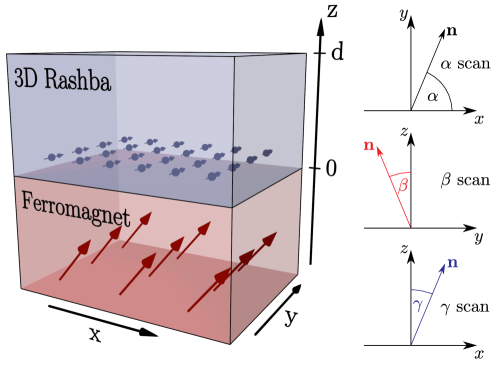
Figure 1: Left: Schematic picture of the setup with a Rashba system (“3D Rashba”) placed on top of a ferromagnetic insulator (“Ferromagnet”). Right: Definition of the angles $\alpha$, $\beta$, and $\gamma$ which describe the rotation of the magnetization direction in the $xy$, $yz$, and $xz$ planes, respectively.

The setup under consideration is schematically depicted in Fig. 1. It consists of a 3D Rashba metal of thickness $d$ which is placed on top of a ferromagnetic insulator with the interface at $z=0$. The ferromagnet offers the possibility to manipulate the spin current across the interface due to the spin transfer torque by varying the magnetization direction $\mathbf{n}$. The boundary condition for the spin current in the Rashba metal at the interface is given byKovalev et al. (2002); Slonczewski (2002)

$$\mathbf{j}_{z}(0)=\frac{1}{2\pi\hbar N_{0}}\left[{g_{r}^{\uparrow\downarrow}}\mathbf{n}\times\big{(}\mathbf{n}\times\mathbf{s}(0)\big{)}+{g_{i}^{\uparrow\downarrow}}\mathbf{n}\times\mathbf{s}(0)\right]\,,$$ (1)

where ${g_{r}^{\uparrow\downarrow}}$ and ${g_{i}^{\uparrow\downarrow}}$ are the real and the imaginary part of the spin mixing conductance. Here, $N_{0}=m_{\parallel}\sqrt{2m_{\perp}\epsilon_{F}}/2\pi^{2}\hbar^{3}$ is the density of states per spin and volume at the Fermi energy of the 3D Rashba metal, which is described by the model Hamiltonian

$$H=\frac{p_{x}^{2}+p_{y}^{2}}{2m_{\parallel}}+\frac{p_{z}^{2}}{2m_{\perp}}-\frac{\alpha_{R}}{\hbar}\left(\mathbf{p}\times\bm{\sigma}\right)\cdot\mathbf{e}_{z}+H_{\mathrm{imp}}\,,$$ (2)

where $\alpha_{R}$ is the Rashba coefficient, and $\bm{\sigma}=(\sigma^{x},\sigma^{y},\sigma^{z})$ is the vector of Pauli matrices. The inversion symmetry breaking direction $\mathbf{e}_{z}$ accounts for the noncentrosymmetric crystal structure. Correspondingly, $m_{\parallel}$ and $m_{\perp}$ are the in-plane and out-of-plane effective masses. Disorder due to nonmagnetic impurities is taken into account by

$$H_{\mathrm{imp}}=V+\frac{\lambda^{2}}{4\hbar}\bm{\sigma}\cdot\left(\nabla V\times\mathbf{p}\right)\,,$$ (3)

where $\lambda$ is the effective Compton wavelength, and $V$ is a $\delta$-correlated random potential.

Based on this microscopic model, we use a generalized Boltzmann equation for the distribution function $f=f^{0}+\mathbf{f}\cdot\bm{\sigma}$ as derived in Ref. Gorini et al., 2010. Here, $f^{0}$ and $\mathbf{f}$ are the charge and the spin distribution functions which yield the spin density

$$\mathbf{s}=\int\frac{d^{3}p}{(2\pi\hbar)^{3}}\mathbf{f}\,,$$ (4)

and the charge and spin current in $i=x,y,z$ direction,

$$j_{i} =-2e\int\frac{d^{3}p}{(2\pi\hbar)^{3}}v_{i}f^{0}\,,$$ (5)

$$\mathbf{j}_{i} =\int\frac{d^{3}p}{(2\pi\hbar)^{3}}v_{i}\mathbf{f}\,,$$ (6)

where $v_{i}$ is the $i$-th component of the velocity $\mathbf{v}=(p_{x}/m_{\parallel},p_{y}/m_{\parallel},p_{z}/m_{\perp})$. For technical details regarding the Boltzmann equation and the derivation of the transport equations used in the following sections we refer to App. A.

Disorder, as taken into account by $H_{\mathrm{imp}}$, leads to momentum relaxation, $1/\tau$, and two types of spin relaxation: Dyakonov-Perel relaxation due to Rashba spin-orbit coupling, and Elliott-Yafet relaxation due to spin-orbit interaction with the random potential. Both relaxation mechanisms are anisotropic,

$$\partial_{t}\mathbf{s}\sim-\frac{1}{\tau_{\textnormal{\tiny DP}}}\begin{pmatrix}1&0&0\\ 0&1&0\\ 0&0&2\end{pmatrix}\mathbf{s}-\frac{1}{\tau_{s}}\begin{pmatrix}1&0&0\\ 0&1&0\\ 0&0&\zeta\end{pmatrix}\mathbf{s}\,,$$ (7)

where $1/\tau_{\textnormal{\tiny DP}}$ and $1/\tau_{s}$ are the Dyakonov-Perel and Elliott-Yafet relaxation rates, respectively. In the dirty regime, the former is given by

$$\frac{1}{\tau_{\textnormal{\tiny DP}}}=\left(\frac{2m_{\parallel}\alpha_{R}}{\hbar^{2}}\right)^{2}D_{\parallel}$$ (8)

with the in-plane diffusion constant $D_{\parallel}=2\epsilon_{F}\tau/3m_{\parallel}$. The anisotropy of the Elliott-Yafet mechanism depends on the masses via the parameter

$$\zeta=\frac{2m_{\perp}}{m_{\perp}+m_{\parallel}}\,,$$ (9)

and the corresponding relaxation rate is given by

$$\frac{1}{\tau_{s}}=\frac{8}{9(2-\zeta)}\left(\frac{\lambda p_{F}}{2\hbar}\right)^{4}\frac{1}{\tau}\,,$$ (10)

with $p_{F}=\sqrt{2m_{\parallel}\epsilon_{F}}$. Note that $\tau_{\textnormal{\tiny DP}}/\tau_{s}\sim\tau^{-2}$ can be enhanced by increasing the temperature, since $\tau^{-1}$ is typically an increasing function of the temperature in a metallic system.

III Current-induced spin polarization

In this section, we investigate the current-induced spin polarization in the spin diffusive limit, in the sense that $p_{F}\tau/m_{\parallel}l_{\textnormal{\tiny DP}}\ll 1$, where $l_{\textnormal{\tiny DP}}=\sqrt{D_{\parallel}\tau_{\textnormal{\tiny DP}}}$. Neglecting spin-dependent contributions to the charge current (thus $j_{x}\approx\sigma_{\mathrm{D}}E_{x}$, where $\sigma_{\mathrm{D}}$ is the Drude conductivity) the Boltzmann equation yields the following set of diffusion equations for the spin density:

$$q_{1}^{2}s^{x} =\nabla_{z}^{2}s^{x}\,,$$ (11)

$$q_{1}^{2}s^{y} =\nabla_{z}^{2}s^{y}+q_{1}^{2}s_{0}^{y}\,,$$ (12)

$$q_{2}^{2}s^{z} =\nabla_{z}^{2}s^{z}\,.$$ (13)

The inverse spin relaxation lengths $q_{1}$ and $q_{2}$ are given by

$$q_{1} =\frac{1}{l_{\textnormal{\tiny DP}}}\sqrt{\frac{m_{\perp}}{m_{\parallel}}\left(1+\frac{\tau_{\textnormal{\tiny DP}}}{\tau_{s}}\right)}\,,$$ (14)

$$q_{2} =\frac{1}{l_{\textnormal{\tiny DP}}}\sqrt{\frac{m_{\perp}}{m_{\parallel}}\left(2+\zeta\frac{\tau_{\textnormal{\tiny DP}}}{\tau_{s}}\right)}\,.$$ (15)

We have also introduced the bulk current-induced spin polarization in the homogeneous case,

$$s_{0}^{y}=-\frac{1}{D_{\parallel}q_{\mathrm{isg}}}\frac{\sigma_{\mathrm{D}}E_{x}}{2e}\,,$$ (16)

where $q_{\mathrm{isg}}$ (“isg” $=$ inverse spin galvanic) is defined by

$$\frac{1}{D_{\parallel}q_{\mathrm{isg}}}=\frac{\tau_{s}/l_{\textnormal{\tiny DP}}}{1+\tau_{s}/\tau_{\textnormal{\tiny DP}}}\left(\xi_{\mathrm{int}}\theta_{\mathrm{int}}^{\mathrm{sH}}+\theta_{\mathrm{ext}}^{\mathrm{sH}}\right)\,.$$ (17)

Here, $\theta_{\mathrm{int}}^{\mathrm{sH}}=\alpha_{R}\tau/\hbar l_{\textnormal{\tiny DP}}$ accounts for the Rashba contribution to the spin Hall angle, and

$$\xi_{\mathrm{int}}=1-\frac{\tau_{\textnormal{\tiny DP}}}{\tau_{s}}\left(1-\frac{3\zeta}{4}\right)\,.$$ (18)

Equation (16) describes the inverse spin galvanic effect in an anisotropic Rashba metal, explicitly taking into account side-jump and skew scattering via the parameter $\theta_{\mathrm{ext}}^{\mathrm{sH}}$, the extrinsic contribution to the spin Hall angle.

To proceed, we explicitly solve Eqs. (11)–(13) by taking into account proper boundary conditions at $z=0$ and $z=d$. These are given by Eq. (1) and the condition $\mathbf{j}_{z}(d)=0$, corresponding to spin-conserving scattering. We obtain

$$s^{y}(z)=s_{0}^{y}+\Delta s_{\mathrm{sc}}^{y}(z)+\Delta s^{y}(z,\mathbf{n})\,,$$ (19)

where

$$\Delta s_{\mathrm{sc}}^{y}(z)=\frac{\theta_{\mathrm{ext}}^{\mathrm{sH}}}{D_{\parallel}q_{1}}\frac{\sigma_{\mathrm{D}}E_{x}}{2e}\frac{\sinh\bm{(}q_{1}(d/2-z)\bm{)}}{\cosh(q_{1}d/2)}$$ (20)

is the spin accumulation which arises due to the spin current $j_{z}^{y}$ even in the absence of the ferromagnet. The magnetization-dependent contribution is given by $\Delta s^{y}(z,\mathbf{n})$. In the following, we focus on $\Delta s^{y}(z,\mathbf{n})$ with the magnetization vector lying in the $xy$, $yz$, or $xz$ plane, respectively, i.e., the $\alpha$, $\beta$, and $\gamma$ scans as defined in Fig. 1. After some algebra, we obtain

$$\Delta s^{y}_{\alpha,\beta,\gamma}(z)=-A(z)f_{\alpha,\beta,\gamma}\,,$$ (21)

with

$$A(z)=s_{0}^{y}\left[1-\tanh\left(q_{1}d/2\right)\theta_{\mathrm{ext}}^{\mathrm{sH}}\frac{q_{\mathrm{isg}}}{q_{1}}\right]\frac{\cosh\bm{(}q_{1}(d-z)\bm{)}}{\cosh(q_{1}d)}\,.$$ (22)

The angular dependence is given by

$$f_{\alpha} =\frac{\left(q_{i}^{2}+q_{r}^{2}+q_{r}\tilde{q}_{2}\right)\cos^{2}\alpha}{q_{i}^{2}+(\tilde{q}_{1}+q_{r})(\tilde{q}_{2}+q_{r})}\,,$$ (23)

$$f_{\beta} =\frac{\left(q_{i}^{2}+q_{r}^{2}+q_{r}\tilde{q}_{1}\right)\cos^{2}\beta}{\frac{\tilde{q}_{1}}{\tilde{q}_{2}}\left[q_{i}^{2}+(\tilde{q}_{1}+q_{r})(\tilde{q}_{2}+q_{r})\right]\sin^{2}\beta+\left[q_{i}^{2}+(\tilde{q}_{1}+q_{r})^{2}\right]\cos^{2}\beta}\,,$$ (24)

$$f_{\gamma} =\frac{q_{i}^{2}+q_{r}^{2}+q_{r}\tilde{q}_{1}-\left(q_{i}^{2}+q_{r}^{2}\right)\left(1-\frac{\tilde{q}_{1}}{\tilde{q}_{2}}\right)\sin^{2}\gamma}{\frac{\tilde{q}_{1}}{\tilde{q}_{2}}\left[q_{i}^{2}+(\tilde{q}_{1}+q_{r})(\tilde{q}_{2}+q_{r})\right]\sin^{2}\gamma+\left[q_{i}^{2}+(\tilde{q}_{1}+q_{r})^{2}\right]\cos^{2}\gamma}\,,$$ (25)

where the respective scan is indicated by the subscript. Furthermore, we have introduced $q_{r,i}=g^{\uparrow\downarrow}_{r,i}/2\pi\hbar N_{0}D_{\perp}$, where $D_{\perp}=2\epsilon_{F}\tau/3m_{\perp}$ is the out-of-plane diffusion constant, and $\tilde{q}_{1,2}=q_{1,2}\tanh(q_{1,2}d)$. An outline of the derivation is given in App. B. Equations (21)–(25) explicitly describe how the spatially resolved spin polarization in an anisotropic Rashba metal depends on the magnetization direction of the adjacent ferromagnet. We wish to point out that these equations fully determine the magnetoresistance signals, as we shall see in the following section.

IV Magnetoresistance

The resistivity $\rho$ is defined by

$$E_{x}=\rho j_{x}\,,$$ (26)

where $E_{x}$ is the electric field, and $j_{x}=1/d\int_{0}^{d}dzj_{x}(z)$ is the current density averaged over the thickness of the Rashba system. In the following, quantities without explicit $z$ dependence are considered as thickness-averaged. Regarding the magnetoresistance, it is convenient to the split the resistivity,

$$\rho=\rho_{0}+\Delta\rho(\mathbf{n})\,,$$ (27)

where $\rho_{0}\approx 1/\sigma_{\mathrm{D}}$ is the resistivity for vanishing spin-mixing conductance, ${g_{r}^{\uparrow\downarrow}}={g_{i}^{\uparrow\downarrow}}=0$, and $\Delta\rho$ captures the magnetization dependence. From the generalized Boltzmann equation, see App. A, one obtains

$$j_{x}(z)=\sigma_{\mathrm{D}}E_{x}+2e\left[\frac{l_{\textnormal{\tiny DP}}}{\tau_{s}}\left(1-\frac{3\zeta}{4}\right)\theta_{\mathrm{int}}^{\mathrm{sH}}s^{y}(z)-\left(\theta_{\mathrm{int}}^{\mathrm{sH}}+\theta_{\mathrm{ext}}^{\mathrm{sH}}\right)j_{y}^{z}(z)+\frac{m_{\perp}}{m_{\parallel}}\theta_{\mathrm{ext}}^{\mathrm{sH}}j_{z}^{y}(z)\right]\,.$$ (28)

Loosely speaking, the first term in the square brackets corresponds to the spin galvanic or inverse Edelstein effect, the second term to the in-plane inverse spin Hall effect, and the third term to the out-of-plane inverse spin Hall effect. Interestingly, the relevant spin currents,

$$j_{y}^{z}(z) =\frac{l_{\textnormal{\tiny DP}}}{\tau_{\textnormal{\tiny DP}}}s^{y}(z)+\left(\theta_{\mathrm{int}}^{\mathrm{sH}}+\theta_{\mathrm{ext}}^{\mathrm{sH}}\right)\frac{\sigma_{\mathrm{D}}E_{x}}{2e}\,,$$ (29)

$$j_{z}^{y}(z) =-D_{\perp}\nabla_{z}s^{y}(z)-\theta_{\mathrm{ext}}^{\mathrm{sH}}\frac{m_{\parallel}}{m_{\perp}}\frac{\sigma_{\mathrm{D}}E_{x}}{2e}\,,$$ (30)

are completely determined by $\Delta s^{y}(z,\mathbf{n})$ regarding their dependence on the magnetization of the ferromagnet. Hence, the angular dependence of $j_{x}(z)$, and thus the magnetoresistance, can be traced back to $\Delta s^{y}(z,\mathbf{n})$.

With the definition of the conductivity, $j_{x}=\sigma E_{x}$, where $\sigma=\sigma_{0}+\Delta\sigma(\mathbf{n})$, analogously to Eq. (27), we obtain

$$\Delta\sigma(\mathbf{n})E_{x}=-2eD_{\parallel}q_{\mathrm{sg}}\Delta s^{y}(\mathbf{n})\,.$$ (31)

Here, we have introduced

$$q_{\mathrm{sg}}=\frac{1}{l_{\textnormal{\tiny DP}}}\Big{[}\xi_{\mathrm{int}}\theta_{\mathrm{int}}^{\mathrm{sH}}+\xi_{\mathrm{ext}}\theta_{\mathrm{ext}}^{\mathrm{sH}}\Big{]}\,,$$ (32)

a wave number which represents the efficiency of the spin galvanic effect, with

$$\xi_{\mathrm{ext}}=1-q_{1}l_{\textnormal{\tiny DP}}\tanh(q_{1}d/2)\,,$$ (33)

and $\xi_{\mathrm{int}}$ as defined in Eq. (18). For a thin system, $q_{1}d\ll 1$, and assuming $q_{1}l_{\textnormal{\tiny DP}}\lesssim 1$, the second term on the r.h.s. of Eq. (33) is negligible. Equivalently, the last term in the square brackets of Eq. (28), after averaging w.r.t. the thickness, is small, which means that the out-of-plane spin current $j_{z}^{y}$ does not contribute to the magnetoresistance, similar to a strictly 2D system.

Assuming $\sigma_{0}\approx\sigma_{\mathrm{D}}\gg\Delta\sigma$, the magnetization-dependent part of the resistivity is given by

$$\frac{\Delta\rho(\mathbf{n})}{\rho_{0}}\approx-\frac{\Delta\sigma(\mathbf{n})}{\sigma_{\mathrm{D}}}\,.$$ (34)

We insert Eq. (31) together with the thickness average of $\Delta s_{\alpha,\beta,\gamma}^{y}(z)$, Eq. (21), and obtain the magnetoresistance ratio

$$\frac{\Delta\rho_{\alpha,\beta,\gamma}}{\rho_{0}}=Cf_{\alpha,\beta,\gamma}$$ (35)

for the $\alpha$, $\beta$, and $\gamma$ scans, respectively. The magnitude of the effect is determined by

$$C=\frac{\tanh(q_{1}d)}{q_{1}d}\frac{q_{\mathrm{sg}}}{q_{\mathrm{isg}}}\left[1-\tanh\left(\frac{q_{1}d}{2}\right)\theta_{\mathrm{ext}}^{\mathrm{sH}}\frac{q_{\mathrm{isg}}}{q_{1}}\right]\,,$$ (36)

with the ratio $q_{\mathrm{sg}}/q_{\mathrm{isg}}$ being quadratic in the spin Hall angles. However, due to the simultaneous contributions from $s^{y}$, $j_{y}^{z}$, and $j^{y}_{z}$, the magnetoresistance cannot generally be expressed in terms of the square of a single total spin Hall angle $\theta_{\mathrm{sH}}$, as in the phenomenological approach.Chen et al. (2013) Only in the special case where intrinsic spin-orbit coupling is negligible, the magnetoresistance can be expressed in terms of a single spin Hall angle squared. In the following, we discuss the magnetoresistance for the representative limits of a purely damping-like torque, ${g_{i}^{\uparrow\downarrow}}=0$, and a purely field-like torque, ${g_{r}^{\uparrow\downarrow}}=0$, respectively.

IV.1 Damping-like torque

In the case of a vanishing imaginary part of the spin mixing conductance, ${g_{i}^{\uparrow\downarrow}}=0$, which corresponds to a damping-like torque, the angular-dependent magnetoresistances are given by

$$\frac{\Delta\rho_{\alpha}}{\rho_{0}} =\frac{Cq_{r}}{q_{r}+\tilde{q}_{1}}\cos^{2}\alpha\,,$$ (37)

$$\frac{\Delta\rho_{\beta}}{\rho_{0}} =\frac{Cq_{r}\cos^{2}\beta}{q_{r}+\tilde{q}_{1}-q_{r}\left(1-\frac{\tilde{q}_{1}}{\tilde{q}_{2}}\right)\sin^{2}\beta}\,,$$ (38)

$$\frac{\Delta\rho_{\gamma}}{\rho_{0}} =\frac{Cq_{r}}{q_{r}+\tilde{q}_{1}}\,.$$ (39)

We see that $\Delta\rho_{\gamma}$ is constant, and that $\Delta\rho_{\beta}$ has a similar angular dependence as $\Delta\rho_{\alpha}$ for a wide range of parameters. More precisely, in the case $|1-\tilde{q}_{1}/\tilde{q}_{2}|\ll 1$, the $\sin^{2}\beta$ term in the denominator in Eq. (38) leads to higher harmonics in $\beta$ of smaller magnitude,

$$\frac{\Delta\rho_{\beta}}{\rho_{0}}\approx\frac{Cq_{r}}{q_{r}+\tilde{q}_{1}}\left[\cos^{2}\beta+\frac{1-\tilde{q}_{1}/\tilde{q}_{2}}{4(1+\tilde{q}_{1}/q_{r})}\sin^{2}(2\beta)\right]\,.$$ (40)

Apparently, the ratio $\tilde{q}_{1}/\tilde{q}_{2}$ determines the sign of the next-to-leading harmonic of the signal.

Figure 2 shows the magnetoresistance according to Eqs. (37)–(39). Panel (a) corresponds to the case where Rashba spin-orbit coupling is large compared to the extrinsic spin-orbit coupling, whereas (b) corresponds to the opposite limit. When Rashba spin-orbit coupling dominates the signal is larger by roughly an order of magnitude as compared to the extrinsic-dominated case. However, the angular dependence is very similar in the two regimes.

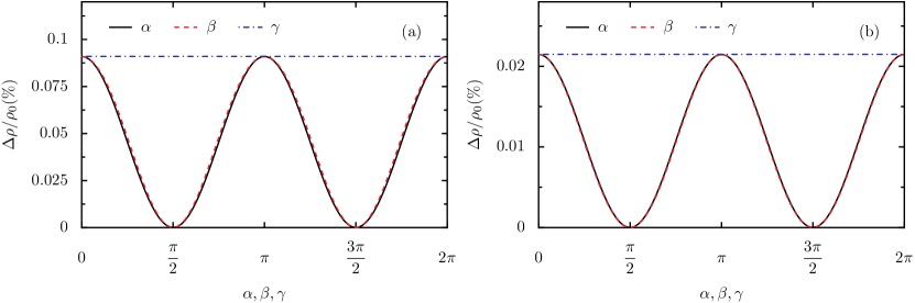
Figure 2: Magnetoresistance for a damping-like torque as function of $\alpha$, $\beta$, and $\gamma$ with $\zeta=0.5$, $q_{r}l_{\textnormal{\tiny DP}}=0.5$, and $d=2l_{\textnormal{\tiny DP}}$. The left panel, (a), corresponds to the case of strong Rashba spin-orbit coupling ($\tau_{\textnormal{\tiny DP}}/\tau_{s}=0.5$, $\theta_{\mathrm{int}}^{\mathrm{sH}}=0.1$, $\theta_{\mathrm{ext}}^{\mathrm{sH}}=0.01$), and the right panel, (b), to the case of dominant extrinsic spin-orbit coupling ($\tau_{\textnormal{\tiny DP}}/\tau_{s}=5$, $\theta_{\mathrm{int}}^{\mathrm{sH}}=0.01$, $\theta_{\mathrm{ext}}^{\mathrm{sH}}=0.1$).

IV.2 Field-like torque

In order to elucidate the effect of a purely field-like torque, we now neglect the real part of the spin mixing conductance, ${g_{r}^{\uparrow\downarrow}}=0$. The angular-dependent magnetoresistances are then given by

$$\frac{\Delta\rho_{\alpha}}{\rho_{0}} =\frac{Cq_{i}^{2}}{q_{i}^{2}+\tilde{q}_{1}\tilde{q}_{2}}\cos^{2}\alpha\,,$$ (41)

$$\frac{\Delta\rho_{\beta}}{\rho_{0}} =\frac{Cq_{i}^{2}\cos^{2}\beta}{q_{i}^{2}+\tilde{q}_{1}^{2}-q_{i}^{2}\left(1-\frac{\tilde{q}_{1}}{\tilde{q}_{2}}\right)\sin^{2}\beta}\,,$$ (42)

$$\frac{\Delta\rho_{\gamma}}{\rho_{0}} =\frac{Cq_{i}^{2}\left[1-\left(1-\frac{\tilde{q}_{1}}{\tilde{q}_{2}}\right)\sin^{2}\gamma\right]}{q_{i}^{2}+\tilde{q}_{1}^{2}-q_{i}^{2}\left(1-\frac{\tilde{q}_{1}}{\tilde{q}_{2}}\right)\sin^{2}\gamma}\,.$$ (43)

The ratio $\tilde{q}_{1}/\tilde{q}_{2}$ defines the sign of the $\sin^{2}\gamma$ contribution in Eq. (43). It also determines whether the ratio of the amplitudes of $\Delta\rho_{\alpha}$ and $\Delta\rho_{\beta}$,

$$\frac{\Delta\rho_{\alpha}(0)}{\Delta\rho_{\beta}(0)}=1-\frac{\tilde{q}_{1}\tilde{q}_{2}}{q_{i}^{2}+\tilde{q}_{1}\tilde{q}_{2}}\left(1-\frac{\tilde{q}_{1}}{\tilde{q}_{2}}\right)\,,$$ (44)

is larger or smaller than one. For $\tilde{q}_{2}\gg q_{i}$ and $\tilde{q}_{1}\gg q_{i}$, Eq. (44) reduces to

$$\frac{\Delta\rho_{\alpha}(0)}{\Delta\rho_{\beta}(0)}\approx\frac{\tilde{q}_{1}}{\tilde{q}_{2}}\,,$$ (45)

such that the ratio $\tilde{q}_{1}/\tilde{q}_{2}$ can be read off directly from the measured amplitudes of the $\alpha$ and $\beta$ signals. Inserting the definitions of $\tilde{q}_{1}$ and $\tilde{q}_{2}$, Eqs. (14) and (15), into Eq. (45), we can solve for

$$\frac{\tau_{\textnormal{\tiny DP}}}{\tau_{s}}=\frac{2\left(\frac{\Delta\rho_{\alpha}(0)}{\Delta\rho_{\beta}(0)}\right)^{2}-1}{1-\zeta\left(\frac{\Delta\rho_{\alpha}(0)}{\Delta\rho_{\beta}(0)}\right)^{2}}\,,$$ (46)

or, in case $\tau_{\textnormal{\tiny DP}}\gg\tau_{s}$, directly extract the anisotropy parameter of the Elliott-Yafet spin relaxation,

$$\zeta\approx\left(\frac{\Delta\rho_{\alpha}(0)}{\Delta\rho_{\beta}(0)}\right)^{-2}\,.$$ (47)

Analogous to the damping-like case, up to linear order in $(1-\tilde{q}_{1}/\tilde{q}_{2})$, we can expand $\Delta\rho_{\beta}$ in terms of harmonics in $\beta$,

$$\frac{\Delta\rho_{\beta}}{\rho_{0}}\approx\frac{Cq_{i}^{2}}{q_{i}^{2}+\tilde{q}_{1}^{2}}\left[\cos^{2}\beta+\frac{1}{4}\left(\frac{1-\tilde{q}_{1}/\tilde{q}_{2}}{1+\tilde{q}_{1}^{2}/q_{i}^{2}}\right)\sin^{2}(2\beta)\right]\,,$$ (48)

and similarly $\Delta\rho_{\gamma}$ can be expressed as

$$\frac{\Delta\rho_{\gamma}}{\rho_{0}}\approx\frac{Cq_{i}^{2}}{q_{i}^{2}+\tilde{q}_{1}^{2}}\left[1-\frac{\tilde{q}_{1}^{2}}{q_{i}^{2}}\left(\frac{1-\tilde{q}_{1}/\tilde{q}_{2}}{1+\tilde{q}_{1}^{2}/q_{i}^{2}}\right)\sin^{2}\gamma\right]\,.$$ (49)

We see that one can obtain the ratio $q_{i}/\tilde{q}_{1}$ by dividing the amplitude of the second-harmonic of $\Delta\rho_{\beta}$ by the amplitude of the $\gamma$ scan of the magnetoresistance.

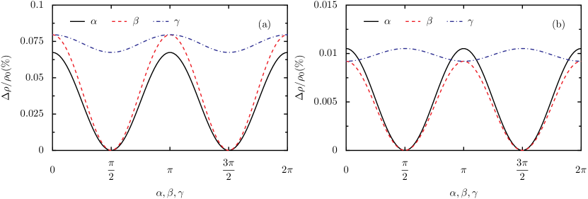
Figure 3: Magnetoresistance for a field-like torque as function of $\alpha$, $\beta$, and $\gamma$ with $\zeta=0.5$, $q_{r}l_{\textnormal{\tiny DP}}=0.5$, and $d=2l_{\textnormal{\tiny DP}}$. The left panel, (a), corresponds to the case of strong Rashba spin-orbit coupling ($\tau_{\textnormal{\tiny DP}}/\tau_{s}=0.5$, $\theta_{\mathrm{int}}^{\mathrm{sH}}=0.1$, $\theta_{\mathrm{ext}}^{\mathrm{sH}}=0.01$), and the right panel, (b), to the case of dominant extrinsic spin-orbit coupling ($\tau_{\textnormal{\tiny DP}}/\tau_{s}=5$, $\theta_{\mathrm{int}}^{\mathrm{sH}}=0.01$, $\theta_{\mathrm{ext}}^{\mathrm{sH}}=0.1$).

IV.3 Discussion

First, we emphasize that our work allows a microscopic description of the magnetoresistance in anisotropic Rashba systems. The theory is not only applicable to real Rashba metals, but also to heavy-metal/ferromagnet bilayers, and substantially extends established phenomenological approaches.Chen et al. (2013) The latter are contained in our results by setting $\zeta=1$, $\alpha_{R}=0$, and $\theta_{\mathrm{ext}}^{\mathrm{sH}}\to\theta_{\mathrm{sH}}$.

Second, we wish to stress the following two aspects: (1) the consideration of a mass anisotropy, and (2) the inclusion of Rashba spin-orbit coupling. The mass anisotropy, point (1), leads to an anisotropic spin relaxation, even in the case of vanishing Rashba spin-orbit coupling $\alpha_{R}=0$, and thus $\tilde{q}_{1}/\tilde{q}_{2}\neq 1$. In this case, according to Eq. (25) the $\gamma$ scan acquires a finite amplitude $\Delta\rho_{\gamma}$ when the imaginary part of the spin mixing conductance is nonzero, ${g_{i}^{\uparrow\downarrow}}\neq 0$. Hence, using a ferromagnetic insulator, one can extract the ratio of the reduced spin relaxation lengths $1/\tilde{q}_{1}$ and $1/\tilde{q}_{2}$ by a precise measurement of $\Delta\rho_{\gamma}$. Indeed, experimental results for a Cu[Pt]/YIG bilayer structure, where the Cu/YIG interface is sputtered with Pt nanosize islands, show a noticeable oscillation in the $\gamma$ scan,Zhou et al. (2018) which can be explained within our theory assuming a nonzero ${g_{i}^{\uparrow\downarrow}}$ and $\tilde{q}_{1}/\tilde{q}_{2}>1$, cf. Fig. 3 (b). This effect is quite pronounced due to an enhancement of the anisotropy of the spin relaxation mechanism as the sputtered Pt exhibits Rashba spin-orbit coupling.Zhou et al. (2018) This directly brings us to point (2). There is evidence that thin Pt films also possess a strong Rashba spin-orbit coupling.Ryu et al. (2016) In this case, the inverse spin galvanic effect strongly influences the spin transport, and the magnetoresistance signal cannot be interpreted as spin Hall magnetoresistance in the sense of a ‘simple’ interplay between the spin Hall and the inverse spin Hall effect, resulting in $\Delta\rho\sim\theta_{\mathrm{sH}}^{2}$. Instead, one should focus on the spin polarization $s^{y}$, described by the wavenumbers $q_{\mathrm{sg}}$ and $q_{\mathrm{isg}}$, which represent the efficiency of the conversion of an electric field to a spin polarization and vice versa. Therefore, our theory is a generalization of previous approachesChen et al. (2013) which focus on the spin Hall angle and the spin currents.

Last but not least, our results compare favorably with experiments on hybrid structures consisting of spin-orbit active materials and a ferromagnetic metal. In these measurements, the $\gamma$ scan is usually explained by an additional contribution from the anisotropic magnetoresistance.Avci et al. (2015); Liu et al. (2015); Kim et al. (2016) Note, however, that the measured signals also qualitatively agree with the magnetoresistance obtained in this work for a field-like torque, see Fig. 3. Since the spin mixing conductance is determined by interface properties, it is not obvious that its imaginary part is always negligible. Therefore, special care is required when interpreting the measured signals. For example, the magnetoresistance in a Bi(15nm)/Ag/CoFeB trilayer, where a Rashba 2DEG is present at the Bi/Ag interface, shows a sign reversal in the oscillation of the $\gamma$ scan when comparing the low-temperature with the room-temperature measurements.Nakayama et al. (2017) Qualitatively, the signals in the first case agree with Fig. 3 (a), and in the second case with Fig. 3 (b). Since $1/\tau$ is typically an increasing function of the temperature and $\tau_{\textnormal{\tiny DP}}/\tau_{s}\sim 1/\tau^{2}$, the ratio $\tilde{q}_{1}/\tilde{q}_{2}$ is also temperature dependent. Hence, Fig. 3 (a) with $\tilde{q}_{1}/\tilde{q}_{2}<1$ due to a small ratio $\tau_{\textnormal{\tiny DP}}/\tau_{s}=0.5$ corresponds to the low-temperature regime and, vice versa, Fig. 3 (b) with $\tilde{q}_{1}/\tilde{q}_{2}>1$ to the high-temperature case.

V Conclusions

We have presented a microscopic theory of the magnetoresistance in bilayer structures consisting of a Rashba metal and a ferromagnetic insulator, where the Rashba metal exhibits a mass anisotropy. Extrinsic spin-orbit coupling due to impurities has been taken into account via Elliott-Yafet spin relaxation, as well as side-jump and skew scattering. The mass anisotropy of the Rashba metal leads to an anisotropic Elliott-Yafet spin relaxation mechanism. Consequently, and enhanced by Dyakonov-Perel spin relaxation, the spin diffusion equations contain two different spin relaxation lengths. Notably, the angular dependence of the magnetoresistance is fully determined by the current-induced spin polarization. In order to illustrate the relevance of the Rashba-metal/ferromagnet interface, we have considered a purely damping-like and a purely field-like torque, respectively. In both cases, the magnitude of the magnetoresistance is strongly enhanced when Rashba spin-orbit coupling is large compared to extrinsic contributions. Interestingly, for a field-like torque the $\gamma$ scan acquires a nonzero amplitude whose sign is determined by the ratio of the two spin relaxation lengths, and is thus directly related to the anisotropy of the spin relaxation. Due to the temperature dependence of the spin relaxation lengths, a sign change in the amplitude of the $\gamma$ scan is predicted which may explain the experimentally observed temperature dependence. A careful analysis of the experimental data will therefore provide important information concerning the anisotropy of the spin relaxation mechanism and its temperature dependence.

Appendix A Kinetic theory

We employ the generalized Boltzmann equation derived in Ref. Gorini et al., 2010. In the static case it reads

$$\frac{i}{\hbar}\frac{\mathbf{p}}{m_{\parallel}}\cdot\left[\bm{\mathcal{A}}^{a}\frac{\sigma^{a}}{2},f\right]+\frac{p_{z}}{m_{\perp}}f+ \frac{1}{2}\left\{\bm{\mathcal{F}}\cdot\nabla_{\mathbf{p}},f\right\}$$

$$=I_{0}+I_{\mathrm{EY}}+I_{\mathrm{ext}}\,.$$ (50)

Here, we have assumed that the system is homogeneous in the $xy$ plane and inhomogeneous for $z>0$ due to the attachment to the ferromagnet at $z=0$. The nonzero components of the SU(2) vector potential and the SU(2) Lorentz force with the electric field $E_{x}\mathbf{e}_{x}$ are given by

$$\mathcal{A}^{x}_{y} =-\mathcal{A}^{y}_{x}=\frac{\hbar}{l_{\textnormal{\tiny DP}}}\,,$$ (51)

$$\bm{\mathcal{F}} =-eE_{x}\mathbf{e}_{x}-\frac{\mathbf{p}}{m_{\parallel}}\times\bm{\mathcal{B}}^{a}\frac{\sigma^{a}}{2}\,,$$ (52)

where the only nonzero component of the SU(2) magnetic field $\mathcal{B}_{i}^{a}$ is $\mathcal{B}_{z}^{z}=-\hbar/l_{\textnormal{\tiny DP}}^{2}$. The collision operators on the r.h.s. of the Boltzmann equation (A) describe momentum relaxation ($I_{0}$) with the relaxation rate $1/\tau$, Elliott-Yafet spin relaxation ($I_{\mathrm{EY}}$) associated with the relaxation rate $1/\tau_{s}$, and side-jump and skew scattering ($I_{\mathrm{ext}}$, see Ref. Raimondi et al., 2012 for details). More precisely, the Elliott-Yafet collision operator consists of

$$I^{0}_{\mathrm{EY}}=-\frac{1}{\tau_{s}}\bm{\sigma}\cdot(\Gamma\langle\mathbf{f}\rangle)\,,$$ (53)

where $\langle\dots\rangle$ denotes the angular average and $\Gamma=\mathrm{diag}(1,1,\zeta)$ accounts for the anisotropy of Elliott-Yafet spin relaxation. In addition, the Elliott-Yafet collision operator yields the following linear in the SU(2) potential contributions:

$$I^{\mathcal{A}}_{\mathrm{EY},s}=\frac{1}{N_{0}\tau}\left(\frac{\lambda}{2\hbar}\right)^{4}\mathcal{A}_{i}^{a}\varepsilon_{ijk}\varepsilon_{lmn}\int\frac{d^{3}p^{\prime}}{(2\pi\hbar)^{3}} \delta(\epsilon_{\mathbf{p}}-\epsilon_{\mathbf{p}^{\prime}})\left(f_{\mathbf{p}^{\prime}}^{0}-f_{\mathbf{p}}^{0}\right)$$

$$\times\left[p^{\prime}_{k}p^{\prime}_{n}p_{m}\delta_{jl}\sigma^{a}-p^{\prime}_{n}p_{k}p_{m}\left(\delta_{aj}\sigma^{l}+\delta_{al}\sigma^{j}-\delta_{jl}\sigma^{a}\right)\right]\,,$$ (54)

$$I^{\mathcal{A}}_{\mathrm{EY},c}=\frac{1}{N_{0}\tau}\left(\frac{\lambda}{2\hbar}\right)^{4}\mathcal{A}_{i}^{a}\varepsilon_{ijk}\varepsilon_{lmn}\int\frac{d^{3}p^{\prime}}{(2\pi\hbar)^{3}} \delta(\epsilon_{\mathbf{p}}-\epsilon_{\mathbf{p}^{\prime}})p^{\prime}_{k}p^{\prime}_{n}p_{m}$$

$$\times\left[f_{\mathbf{p}^{\prime}}^{b}(\delta_{al}\delta_{bj}+\delta_{aj}\delta_{bl})-\delta_{ab}\delta_{jl}\left(f_{\mathbf{p}^{\prime}}^{b}+f_{\mathbf{p}}^{b}\right)\right]\,,$$ (55)

where $\epsilon_{\mathbf{p}}=(p_{x}^{2}+p_{y}^{2})/2m_{\parallel}+p^{2}_{z}/m_{\perp}$ is the band energy and $s$ ($c$) denotes a contribution to the spin (charge) sector. The above collision operators, Eqs. (53)–(55), are obtained by following the outline given in Ref. Gorini et al., 2010 with the self-energies

$$\tilde{\Sigma}^{0}_{\mathrm{EY}}= \frac{1}{2\pi\hbar N_{0}\tau}\left(\frac{\lambda}{2\hbar}\right)^{4}\int\frac{d^{3}p^{\prime}}{(2\pi\hbar)^{3}}\left[\left(\mathbf{p}\times\mathbf{p}^{\prime}\right)\cdot\bm{\sigma}\right]\tilde{G}(\mathbf{p}^{\prime})\left[\left(\mathbf{p}\times\mathbf{p}^{\prime}\right)\cdot\bm{\sigma}\right]\,,$$ (56)

$$\tilde{\Sigma}^{\mathcal{A}}_{\mathrm{EY}}= \frac{1}{4\pi\hbar N_{0}\tau}\left(\frac{\lambda}{2\hbar}\right)^{4}\big{\{}\mathcal{A}_{i}^{a}\sigma^{a},\nabla_{p_{i}}\int\frac{d^{3}p^{\prime}}{(2\pi\hbar)^{3}}\left[\left(\mathbf{p}\times\mathbf{p}^{\prime}\right)\cdot\bm{\sigma}\right]\tilde{G}(\mathbf{p}^{\prime})\left[\left(\mathbf{p}\times\mathbf{p}^{\prime}\right)\cdot\bm{\sigma}\right]\big{\}}$$

$$-\frac{1}{4\pi\hbar N_{0}\tau}\left(\frac{\lambda}{2\hbar}\right)^{4}\int\frac{d^{3}p^{\prime}}{(2\pi\hbar)^{3}}\left[\left(\mathbf{p}\times\mathbf{p}^{\prime}\right)\cdot\bm{\sigma}\right]\big{\{}\mathcal{A}_{i}^{a}\sigma^{a},(\nabla_{p^{\prime}_{i}}\tilde{G}(\mathbf{p}^{\prime}))\big{\}}\left[\left(\mathbf{p}\times\mathbf{p}^{\prime}\right)\cdot\bm{\sigma}\right]\,,$$ (57)

where $\{\cdot,\cdot\}$ denotes the anti-commutator and $\tilde{G}$ is the locally covariant Green’s function in Keldysh space. Although not explicitly indicated, the self-energies and Green’s function are taken as impurity averaged, $\langle V(\mathbf{r})V(\mathbf{r}^{\prime})\rangle_{\mathrm{imp}}=(\hbar/2\pi N_{0}\tau)\delta(\mathbf{r}-\mathbf{r}^{\prime})$. For more details on the Elliott-Yafet collision operator we refer, for instance, to Refs. Tölle et al., 2017; Gorini et al., 2017.

By performing the trace of the Boltzmann equation (A), multiplying with $p_{x}$, performing the momentum integration, and rearranging the terms one obtains the charge current $j_{x}$ as given in Eq. (28). In order to derive the spin diffusion equations (11)–(13) we consider the trace of the Boltzmann equation after multiplication with the Pauli vector, $\mathrm{Tr}[\bm{\sigma}/2\dots]$. From the resulting $3\times 3$ matrix equation we can obtain two equations for the spin density and the spin current: first, a direct integration over the momentum yields

$$\Gamma\mathbf{s}+\tau_{s}\nabla_{z}\mathbf{j}_{z}-\tau_{s}\frac{\bm{\mathcal{A}}_{i}}{\hbar}\times\mathbf{j}_{i}=\mathbf{e}_{y}\theta^{\mathrm{sH}}_{\mathrm{int}}\frac{\tau_{\textnormal{\tiny DP}}}{l_{\textnormal{\tiny DP}}}\left(1-\frac{3\zeta}{4}\right)\frac{\sigma_{\mathrm{D}}E_{x}}{2e}\,.$$ (58)

Second, solving for $\mathbf{f}$ in terms of $\langle\mathbf{f}\rangle$ and $f^{0}$, and performing the momentum integration after a multiplication by $p_{i}$ with $i=x,y,z$ yields the spin currents

$$\mathbf{j}_{x} =-\frac{l_{\textnormal{\tiny DP}}}{\tau_{\textnormal{\tiny DP}}}\mathbf{e}_{y}\times\mathbf{s}\,,$$ (59)

$$\mathbf{j}_{y} =\frac{l_{\textnormal{\tiny DP}}}{\tau_{\textnormal{\tiny DP}}}\mathbf{e}_{x}\times\mathbf{s}+\mathbf{e}_{z}\left(\theta^{\mathrm{sH}}_{\mathrm{int}}+\theta^{\mathrm{sH}}_{\mathrm{ext}}\right)\frac{\sigma_{\mathrm{D}}E_{x}}{2e}\,,$$ (60)

$$\mathbf{j}_{z} =-D_{\perp}\nabla_{z}\mathbf{s}-\mathbf{e}_{y}\theta^{\mathrm{sH}}_{\mathrm{ext}}\frac{m_{\parallel}}{m_{\perp}}\frac{\sigma_{\mathrm{D}}E_{x}}{2e}\,.$$ (61)

The spin diffusion equations (11)–(13) now follow from inserting Eqs. (59)–(61) into Eq. (58).

Appendix B Spin diffusion equations

In this appendix we briefly outline how to solve the spin diffusion equations (11)–(13) for the current-induced spin polarization $s^{y}$ as described by Eqs. (19)–(25). Since we deal with decoupled differential equations, the general solution is easily obtained,

$$s^{x} =a_{1}e^{-q_{1}z}+a_{2}e^{q_{1}z}\,,$$ (62)

$$s^{y} =b_{1}e^{-q_{1}z}+b_{2}e^{q_{1}z}+s_{0}^{y}\,,$$ (63)

$$s^{z} =c_{1}e^{-q_{2}z}+c_{2}e^{q_{2}z}\,,$$ (64)

respectively. The boundary conditions as given in the main text, $\mathbf{j}_{z}(d)=0$ and Eq. (1), can be applied to Eqs. (62)–(64) by employing Eq. (61). Considering first $\mathbf{j}_{z}(d)=0$, we can reduce the number of unknown parameters,

$$s^{x} =a\cosh\bm{(}q_{1}(d-z)\bm{)}\,,$$ (65)

$$s^{y} =b\cosh\bm{(}q_{1}(d-z)\bm{)}+\frac{\theta^{\mathrm{sH}}_{\mathrm{ext}}\sigma_{\mathrm{D}}E_{x}}{2eq_{1}D_{\parallel}}\sinh\bm{(}q_{1}(d-z)\bm{)}+s_{0}^{y}\,,$$ (66)

$$s^{z} =c\cosh\bm{(}q_{2}(d-z)\bm{)}\,.$$ (67)

It is now convenient to consider first the case without ferromagnet, i.e., $\mathbf{j}_{z}(0)=0$. In this case, the spin density $s^{y}$ is given by

$$s^{y}(z)\big{|}_{q_{r}=q_{i}=0}=s_{0}^{y}+\Delta s^{y}_{sc}(z)\,,$$ (68)

with $\Delta s^{y}_{sc}$ as given in Eq. (20). In the presence of the ferromagnet, the spin density can be written as follows:

$$\mathbf{s}(z,\mathbf{n})=\left[s^{y}_{0}+\Delta s_{\mathrm{sc}}^{y}(z)\right]\mathbf{e}_{y}+\Delta\mathbf{s}(z,\mathbf{n})\,,$$ (69)

where

$$\Delta\mathbf{s}(z,\mathbf{n})=\begin{pmatrix}\tilde{a}\cosh\bm{(}q_{1}(d-z)\bm{)}\\ \tilde{b}\cosh\bm{(}q_{1}(d-z)\bm{)}\\ \tilde{c}\cosh\bm{(}q_{2}(d-z)\bm{)}\end{pmatrix}\,.$$ (70)

By splitting the spin current $\mathbf{j}_{z}$ similar to Eq. (69), the application of the boundary condition (1) leads to

$$\begin{pmatrix}q_{1}\tilde{a}\sinh(q_{1}d)\\ q_{1}\tilde{b}\sinh(q_{1}d)\\ q_{1}\tilde{c}\sinh(q_{2}d)\end{pmatrix}= D_{\perp}q_{r}\mathbf{n}\times\big{[}\mathbf{n}\times\mathbf{s}(z=0)\big{]}$$

$$+D_{\perp}q_{i}\mathbf{n}\times\mathbf{s}(z=0)$$ (71)

with

$$\mathbf{s}(z=0)=\left[s^{y}_{0}+\Delta s_{\mathrm{sc}}^{y}(0)\right]\mathbf{e}_{y}+\begin{pmatrix}\tilde{a}\cosh(q_{1}d)\\ \tilde{b}\cosh(q_{1}d)\\ \tilde{c}\cosh(q_{2}d)\end{pmatrix}\,.$$ (72)

The remaining task is now to solve for $\tilde{b}$. One way is to parametrize $\mathbf{n}$ in spherical coordinates and multiply Eq. (71) by the rotation matrix $\mathbb{D}$ with the property $\mathbb{D}\mathbf{n}=\mathbf{e}_{x}$. By a proper choice of the spherical angles regarding the $\alpha$, $\beta$, and $\gamma$ scans, respectively, the solution for $\tilde{b}$ of the resulting system of linear equations finally yields the spin density $\Delta s^{y}_{\alpha,\beta,\gamma}$ as given by Eqs. (21)–(25).

References

• $\check{\textnormal{Z}}$utić et al. (2004) I. $\check{\textnormal{Z}}$utić, J. Fabian,  and S. Das Sarma, Rev. Mod. Phys. 76, 323 (2004).
• Sinova et al. (2015) J. Sinova, S. O. Valenzuela, J. Wunderlich, C. H. Back,  and T. Jungwirth, Rev. Mod. Phys. 87, 1213 (2015).
• Nakayama et al. (2013) H. Nakayama, M. Althammer, Y.-T. Chen, K. Uchida, Y. Kajiwara, D. Kikuchi, T. Ohtani, S. Geprägs, M. Opel, S. Takahashi, R. Gross, G. E. W. Bauer, S. T. B. Goennenwein,  and E. Saitoh, Phys. Rev. Lett. 110, 206601 (2013).
• Avci et al. (2015) C. O. Avci, K. Garello, A. Ghosh, M. Gabureac, S. F. Alvarado,  and P. Gambardella, Nat. Phys. 11, 570 (2015).
• Han et al. (2014) J. H. Han, C. Song, F. Li, Y. Y. Wang, G. Y. Wang, Q. H. Yang,  and F. Pan, Phys. Rev. B 90, 144431 (2014).
• Dyakonov and Perel (1971) M. Dyakonov and V. Perel, Phys. Lett. A 35, 459 (1971).
• Hirsch (1999) J. E. Hirsch, Phys. Rev. Lett. 83, 1834 (1999).
• Kato et al. (2004a) Y. K. Kato, R. C. Myers, A. C. Gossard,  and D. D. Awschalom, Science 306, 1910 (2004a).
• Wunderlich et al. (2005) J. Wunderlich, B. Kaestner, J. Sinova,  and T. Jungwirth, Phys. Rev. Lett. 94, 047204 (2005).
• Slonczewski (1996) J. Slonczewski, J. Magn. Magn. Mater. 159, L1 (1996).
• Berger (1996) L. Berger, Phys. Rev. B 54, 9353 (1996).
• Tsoi et al. (1998) M. Tsoi, A. G. M. Jansen, J. Bass, W.-C. Chiang, M. Seck, V. Tsoi,  and P. Wyder, Phys. Rev. Lett. 80, 4281 (1998).
• Zhao et al. (2006) H. Zhao, E. J. Loren, H. M. van Driel,  and A. L. Smirl, Phys. Rev. Lett. 96, 246601 (2006).
• Saitoh et al. (2006) E. Saitoh, M. Ueda, H. Miyajima,  and G. Tatara, Appl. Phys. Lett. 88, 182509 (2006).
• Valenzuela and Tinkham (2006) S. O. Valenzuela and M. Tinkham, Nature 442, 176 (2006).
• Nakayama et al. (2016) H. Nakayama, Y. Kanno, H. An, T. Tashiro, S. Haku, A. Nomura,  and K. Ando, Phys. Rev. Lett. 117, 116602 (2016).
• Nakayama et al. (2017) H. Nakayama, H. An, A. Nomura, Y. Kanno, S. Haku, Y. Kuwahara, H. Sakimura,  and K. Ando, Appl. Phys. Lett. 110, 222406 (2017).
• Ivchenko and Pikus (1978) E. L. Ivchenko and G. E. Pikus, JETP Lett. 27, 604 (1978).
• Vas’ko and Prima (1979) F. T. Vas’ko and N. A. Prima, Sov. Phys. Solid State 21, 994 (1979).
• Aronov and Lyanda-Geller (1989) A. G. Aronov and Y. B. Lyanda-Geller, JETP Lett. 50, 431 (1989).
• Kato et al. (2004b) Y. K. Kato, R. C. Myers, A. C. Gossard,  and D. D. Awschalom, Phys. Rev. Lett. 93, 176601 (2004b).
• Silov et al. (2004) A. Y. Silov, P. A. Blajnov, J. H. Wolter, R. Hey, K. H. Ploog,  and N. S. Averkiev, Appl. Phys. Lett. 85, 5929 (2004).
• Edelstein (1990) V. Edelstein, Solid State Commun. 73, 233 (1990).
• Rashba (1960) É. I. Rashba, Sov. Phys. Solid State 2, 1109 (1960).
• Bychkov and Rashba (1984) Y. A. Bychkov and É. I. Rashba, JETP Lett. 39, 78 (1984).
• Ganichev et al. (2001) S. D. Ganichev, E. L. Ivchenko, S. N. Danilov, J. Eroms, W. Wegscheider, D. Weiss,  and W. Prettl, Phys. Rev. Lett. 86, 4358 (2001).
• Ganichev et al. (2002) S. D. Ganichev, E. L. Ivchenko, V. V. Bel’kov, S. A. Tarasenko, M. Sollinger, D. Weiss, W. Wegscheider,  and W. Prettl, Nature 417, 153 (2002).
• Raimondi et al. (2012) R. Raimondi, P. Schwab, C. Gorini,  and G. Vignale, Ann. Phys. (Berlin) 524, 153 (2012).
• Grigoryan et al. (2014) V. L. Grigoryan, W. Guo, G. E. W. Bauer,  and J. Xiao, Phys. Rev. B 90, 161412 (2014).
• Tölle et al. (2017) S. Tölle, U. Eckern,  and C. Gorini, Phys. Rev. B 95, 115404 (2017).
• Tölle et al. (2018) S. Tölle, M. Dzierzawa, U. Eckern,  and C. Gorini, Ann. Phys. (Berlin) 530, 1700303 (2018).
• Ishizaka et al. (2011) K. Ishizaka, M. S. Bahramy, H. Murakawa, M. Sakano, T. Shimojima, T. Sonobe, K. Koizumi, S. Shin, H. Miyahara, A. Kimura, et al., Nat. Mater. 10, 521 (2011).
• Niesner et al. (2016) D. Niesner, M. Wilhelm, I. Levchuk, A. Osvet, S. Shrestha, M. Batentschuk, C. Brabec,  and T. Fauster, Phys. Rev. Lett. 117, 126401 (2016).
• Martin et al. (2017) C. Martin, A. V. Suslov, S. Buvaev, A. F. Hebard, P. Bugnon, H. Berger, A. Magrez,  and D. B. Tanner, EPL 116, 57003 (2017).
• Brosco and Grimaldi (2017) V. Brosco and C. Grimaldi, Phys. Rev. B 95, 195164 (2017).
• Chen et al. (2013) Y.-T. Chen, S. Takahashi, H. Nakayama, M. Althammer, S. T. B. Goennenwein, E. Saitoh,  and G. E. W. Bauer, Phys. Rev. B 87, 144411 (2013).
• Kovalev et al. (2002) A. A. Kovalev, A. Brataas,  and G. E. W. Bauer, Phys. Rev. B 66, 224424 (2002).
• Slonczewski (2002) J. C. Slonczewski, J. Magn. Magn. Mater. 247, 324 (2002).
• Gorini et al. (2010) C. Gorini, P. Schwab, R. Raimondi,  and A. L. Shelankov, Phys. Rev. B 82, 195316 (2010).
• Note (1) A brief outline of the Elliott-Yafet spin relaxation as described within the Boltzmann theory is given in App. A.
• Note (2) Note that $\theta_{\mathrm{int}}^{\mathrm{sH}}$ is not the bulk spin Hall angle in case of a pure Rashba system.Raimondi et al. (2012).
• Note (3) More precisely, $\theta_{\mathrm{ext}}^{\mathrm{sH}}=\theta_{\mathrm{sj}}^{\mathrm{sH}}+\theta_{\mathrm{ss}}^{\mathrm{sH}}$, where $\theta_{\mathrm{sj,ss}}^{\mathrm{sH}}=2e\sigma_{\mathrm{sj,ss}}^{\mathrm{sH}}/\sigma_{\mathrm{D}}$ with the side-jump and skew scattering contributions to the spin Hall conductivity, $\sigma_{\mathrm{sj}}^{\mathrm{sH}}$ and $\sigma_{\mathrm{ss}}^{\mathrm{sH}}$, being defined in Ref. \rev@citealpnumraimondi2012, respectively.
• Zhou et al. (2018) L. Zhou, H. Song, K. Liu, Z. Luan, P. Wang, L. Sun, S. Jiang, H. Xiang, Y. Chen, J. Du, et al., Sci. Adv. 4, eaao3318 (2018).
• Ryu et al. (2016) J. Ryu, M. Kohda,  and J. Nitta, Phys. Rev. Lett. 116, 256802 (2016).
• Liu et al. (2015) J. Liu, T. Ohkubo, S. Mitani, K. Hono,  and M. Hayashi, Appl. Phys. Lett. 107, 232408 (2015).
• Kim et al. (2016) J. Kim, P. Sheng, S. Takahashi, S. Mitani,  and M. Hayashi, Phys. Rev. Lett. 116, 097201 (2016).
• Gorini et al. (2017) C. Gorini, A. Maleki Sheikhabadi, K. Shen, I. V. Tokatly, G. Vignale,  and R. Raimondi, Phys. Rev. B 95, 205424 (2017).