On stability properties of the Cubic-Quintic Schrödinger equation with $\delta$-point interaction

Abstract

We study analytically and numerically the existence and orbital stability of the peak-standing-wave solutions for the cubic-quintic nonlinear Schrödinger equation with a point interaction determined by the delta of Dirac. We study the cases of attractive-attractive and attractive-repulsive nonlinearities and we recover some results in the literature. Via a perturbation method and continuation argument we determine the Morse index of some specific self-adjoint operators that arise in the stability study. Orbital instability implications from a spectral instability result are established. In the case of an attractive-attractive case and an focusing interaction we give an approach based in the extension theory of symmetric operators for determining the Morse index.

Mathematics Subject Classification (2000). Primary 35Q51, 35J61; Secondary 47E05.
Key words. Nonlinear stability of peak-solutions, nonlinear Schrödinger equation with point interaction, analytic perturbation theory, self-adjoint extensions.

1 Introduction

This work addresses the nonlinear stability and instability properties of peak-standing wave associated to the following cubic-quintic nonlinear Schrödinger equation with a point interaction determined by Dirac $\delta$ distribution centered at the origem (henceforth NLSCQ),

$$iu_{t}+u_{xx}+Z\delta(x)u+\lambda_{1}|u|^{2}u+\lambda_{2}|u|^{4}u=0,\quad\text{for}\;\;t,x\in\mathbb{R},$$ (1)

here $u=u(x,t)\in\mathbb{C}$, $\lambda_{i}\in\mathbb{R}$, and $Z\in\mathbb{R}$ represents the so-called strength parameter.

Equation NLSCQ represents a very general family of models featuring the competition between repulsive ($\lambda_{1}\leqq 0$)/attractive ($\lambda_{1}\geqq 0$) cubic and repulsive ($\lambda_{2}\leqq 0$)/attractive ($\lambda_{2}\geqq 0$)/quintic terms, together with a point interaction or defect determined by the $\delta$ distribution at the origem. That models with $Z=0$, it have drawn considerable attention in the last years by its physical relevance in optical media, liquid waveguides and others ([18], [26], [27], [32]). The case $\lambda_{2}=0$ and $Z\neq 0$ has been also studied substantially in the literature (see [4], [9], [13], [17], [21], [23], [24], [28], [29], [33], [37], [38] and references therein). The case of Schrödinger models on star graphs with $\delta$ conditions on the vertex also have been studied recently in Adami et. al ([1], [2] and references therein) and Angulo&Goloshchapova ([11], [12], [13]). The case of either other defect type or nonlinearity have been studied in [4], [10], [13], [14]. The specific case $\lambda_{1}=2$, $\lambda_{2}=-1$ and $Z>0$ was recently considered by Genoud&Malomed&Weishaupl in [31].

The combination of nonlinearities in (1) is well known in optical media ([26], [27], [18]). In particular, we recall that for a effective linear potential term, $V(x)$, the general NLS model

$$iu_{t}+u_{xx}+V(x)u+F(u)=0$$

represents a trapping (wave-guiding) structure for light beams, induced by an inhomogeneity of the local refractive index. In particular, the delta-function term in NLSCQ adequately represents a narrow trap which is able to capture broad solitonic beams.

The focus of this manuscript is the existence and stability properties of standing-wave solutions for the model NLSCQ, namely, solutions in the form

$$u(x,t)=e^{-i\omega t}\phi_{\omega}(x),\;\;\;\;\;\;\;\;\omega\in I\subset\mathbb{R},$$ (2)

where $I$ is an interval and the profile $\phi_{\omega}:\mathbb{R}\to\mathbb{R}$ belongs to the domain of the quantum operator $-\partial_{x}^{2}-Z\delta(x)$, more exactly, for

$$\phi_{\omega}\in D(-\partial_{x}^{2}-Z\delta(x))=\{f\in H^{1}(\mathbb{R})\cap H^{2}(\mathbb{R}-\{0\}):f^{\prime}(0+)-f^{\prime}(0-)=-Zf(0)\}.$$

Thus, we have for $x\neq 0$, that the profile $\phi_{\omega}$ satisfies the elliptic equation

$$\phi^{\prime\prime}_{\omega}(x)-\omega\phi_{\omega}(x)-\lambda_{1}\phi^{3}_{\omega}(x)-\lambda_{2}\phi^{5}_{\omega}(x)=0.$$ (3)

The existence of solutions for equation (3) have been considered in analytic, numerical and experimental works for specific values of the parameters $Z,\omega,\lambda_{1},\lambda_{2}$. For $Z=0$, the rigorous existence and stability analysis of standing waves for NLSCQ model with general double-power nonlinearities can be found in [42]-[46]. The existence and stability for $\lambda_{1}\neq 0$, $\lambda_{2}=0$, $\omega<0$, $Z\neq 0$, and with the cubic nonlinearity term changed by the single power-law nonlinearity $|\phi_{\omega}|^{p-1}\phi_{\omega}$, $p>1$, have been extensively discussed earlier in [13], [23], [28], [29], [33], [38]. In a periodic framework, we have the recents works of Angulo [9] and Angulo&Ponce [17].

Now, it is well-known that for arbitrary values of $\lambda_{1}$ and $\lambda_{2}$, NSLCQ model can not have standing-wave solutions vanishing at the infinity (still in the case $Z=0$). Moreover, in the case of the existence of solutions may happened that exact solutions are not available in general. Recently, Genoud&Malomed&Weishaupl in [31] have studied the stability of a family of explicit standing-wave solutions for NLSCQ model with a combination of an attractive ($\lambda_{1}=2$) and repulsive ($\lambda_{2}=-1$) nonlinearities, and with a focusing $\delta$-interaction, $Z\in(0,\sqrt{3})$, such that the wave phase velocity $-\omega$ satisfies $-\omega\in(\frac{Z^{2}}{4},\frac{3}{4}+\frac{Z^{2}}{4})$. Here, we extend and complete some of the results in [31] and we determine the profile for (3) in the cases attractive-attractive and attractive-repulsive.

The peak-standing-wave solutions for NLSCQ model which we are interested here the following:

1. atractive-atractive ($\lambda_{1},\lambda_{2}>0$): the parameters $\omega$ and $Z$ in (3) will satisfy that $\omega<0$, $Z\in\mathbb{R}$, and the condition $-\omega>\frac{Z^{2}}{4}$. Thus, we have the profile $\phi_{\omega}=\phi_{\omega,Z,\lambda_{1},\lambda_{2}}$ for $\alpha=\frac{\lambda_{1}}{4}$ and $\beta=\frac{\lambda_{2}}{3}$

   $$\phi_{\omega}(x)=\left[-\frac{\alpha}{\omega}+\frac{\sqrt{\alpha^{2}-\beta\omega}}{-\omega}\cosh\left(2\sqrt{-\omega}\left(|x|+R^{-1}\left(\frac{Z}{2\sqrt{-\omega}}\right)\right)\right)\right]^{-\frac{1}{2}}$$ (4)

   with $R:(-\infty,\infty)\rightarrow(-1,1)$ being the diffeomorphism defined by

   $$R(s)=\frac{\sqrt{\alpha^{2}-\beta\omega}\sinh(2\sqrt{-\omega}s)}{\alpha+\sqrt{\alpha^{2}-\beta\omega}\cosh(2\sqrt{-\omega}s)}.$$ (5)

   We note that for every $\lambda_{2}>0$, the expression $\sqrt{\alpha^{2}-\beta\omega}$ is well-defined.

2. attractive-repulsive ($\lambda_{1}>0$, $\lambda_{2}<0$): the profile $\phi_{\omega}$ in (4) is still a solution for (3), but we have the following restriction of parameters,

   $$\frac{Z^{2}}{4}<-\omega<-\frac{3\lambda_{1}^{2}}{16\lambda_{2}},\qquad|Z|<\frac{\sqrt{3}\lambda_{1}}{2\sqrt{-\lambda_{2}}}.$$ (6)

Figure 1 below shows the profile of $\phi_{\omega}$ for $\lambda_{1}=\lambda_{2}=1$ with $Z>0$ and $Z<0$. Now, for the case of repulsive nonlinearities ($\lambda_{1},\lambda_{2}<0$) and $Z<0$, by using a Pohazev type argument we can show the nonexistence of nontrivial solutions for (3) vanishing at the infinity.

Theorem 1 and Theorem 2, below, establish our stability results associated to the profile $\phi_{\omega}$ in (4) for the cases $\lambda_{1},\lambda_{2}>0$ and $\lambda_{1}>0$, $\lambda_{2}<0$. We note that in the case attractive-repulsive, we extend the results in [31].

Now, the basic symmetry associated to equation (1) is the phase-invariance, since the translation invariance of the solutions is not hold due to the defect. Thus, our notion of stability (instability) will be based with regard to this symmetry and it is formulated as follows: For $\eta>0$, let $\phi$ be a solution of (3) and define the neighborhood

$$U_{\eta}(\phi)=\Big{\{}v\in X:\inf_{\theta\in\mathbb{R}}\|v-e^{i\theta}\phi\|_{X}<\eta\Big{\}}.$$

Definition 1.

The standing wave $e^{-i\omega t}\phi$ is (orbitally) stable by the flow of the NLSCQ model (1) in $X$ if for any $\epsilon>0$ there exists $\eta>0$ such that for any $u_{0}\in U_{\eta}(\phi)$, the solution $u(t)$ of (1) with $u(0)=u_{0}$ satisfies $u(t)\in U_{\epsilon}(\phi)$ for all $t\in\mathbb{R}$. Otherwise, $e^{-i\omega t}\phi$ is said to be (orbitally) unstable in $X$.

The space $X$ in Definition 1 will be considered in our stability theory being as $H^{1}(\mathbb{R})$ or $H_{even}^{1}(\mathbb{R})$ (The space of even fuctions on $H^{1}(\mathbb{R})$). Thus, our main stability results for the peak-standing-wave profiles in (4) are the following.

Theorem 1.

For $\lambda_{1}=\lambda_{2}=1$ and $Z^{*}\approx-0.866025403784$, we have for $\omega<0$ such that $-\omega>\frac{Z^{2}}{4}$ and $\phi_{\omega}$ defined in (4) the following:

1. For $Z\geq 0$, $e^{-i\omega t}\phi_{\omega,Z}$ is orbitally stable in $H^{1}(\mathbb{R})$.

2. For $Z\in(Z^{*},0)$, $e^{-i\omega t}\phi_{\omega,Z}$ is orbitally unstable in $H^{1}(\mathbb{R})$.

3. For $Z\in(Z^{*},\infty)$, $e^{-i\omega t}\phi_{\omega,Z}$ is orbitally stable in $H_{even}^{1}(\mathbb{R})$.

4. For $Z<Z^{*}$, $e^{-i\omega t}\phi_{\omega,Z}$ is orbitally unstable in $H_{even}^{1}(\mathbb{R})$ and so in $H^{1}(\mathbb{R})$.

Remark 1.

Our numerical simulations (see Figures 2, 3 and 4 below) showed us that to find exactly the threshold value $Z^{*}$ such that the mapping $\omega\to-\|\phi_{\omega,Z^{*}}\|^{2}$ has a only critical point can be very tricky, but it is possible to see that in the neighborhood of $Z^{*}$ that map does not oscillate. In Theorem 1 we consider the specific attractive-values $\lambda_{1}=\lambda_{2}=1$ due to the complexity of the formulas appearing in the analysis established in Section 5 below. But, our numerical simulations showed that a similar stability behavior of the profile $\phi_{\omega}$ is obtained for $\lambda_{1},\lambda_{2}>0$ and a threshold value of $Z$, $Z^{*}=Z^{*}(\lambda_{1},\lambda_{2})$.

Theorem 2.

Let $\lambda_{1}>0$ and $\lambda_{2}<0$. Then, for $\omega<0$ and $Z\in\mathbb{R}$ such that

$$\frac{Z^{2}}{4}<-\omega<-\frac{3\lambda_{1}^{2}}{16\lambda_{2}},\qquad|Z|<\frac{\sqrt{3}\lambda_{1}}{2\sqrt{-\lambda_{2}}},$$

we have that $\phi_{\omega}$ defined in (4) has the following property:

1. For $0<Z<\frac{\sqrt{3}\lambda_{1}}{2\sqrt{-\lambda_{2}}}$, $e^{-i\omega t}\phi_{\omega,Z}$ is orbitally stable in $H^{1}(\mathbb{R})$.

2. For $-\frac{\sqrt{3}\lambda_{1}}{2\sqrt{-\lambda_{2}}}<Z<0$, $e^{-i\omega t}\phi_{\omega,Z}$ is orbitally unstable in $H^{1}(\mathbb{R})$.

3. For $-\frac{\sqrt{3}\lambda_{1}}{2\sqrt{-\lambda_{2}}}<Z<0$, $e^{-i\omega t}\phi_{\omega,Z}$ is orbitally stable in $H_{even}^{1}(\mathbb{R})$.

Remark 2.

The stability result in item a) -Theorem 2 with the specific restrictions $\lambda_{1}=2$, $\lambda_{2}=-1$, $\frac{Z^{2}}{4}<-\omega<\frac{3}{4}$, and $Z\in(0,\sqrt{3})$, it was obtained recently by Genoud&Malomed&Weishaupl in [31].

Our approach for proving Theorem 1 and Theorem 2 will be based in the general framework developed by Grillakis&Shatah&Strauss [34]-[35], for a Hamiltonian system which is invariant under a one-parameter unitary group of operators. We recall that this approach requires spectral analysis of certain self-adjoint Schrödinger operator and in particular by determining the Morse index is one of the more delicate issues in the approach. In particular, our strategy will be based in analytic perturbation theory. Now for $Z>0$, we present a new approach for obtaining that index based in the extension theory of symmetric operators by von Neumann and Krein (see Appendix).

We also note that for applying the instability criterium in [35] in our case (initially being of spectral instability), we need to justify nonlinear instability from a spectral instability behavior (see Remark 7). We note that our argument (spectral instability $\to$ nonlinear instability) complements several instability results in the literature for the case $\lambda_{2}=0$ in (1).

This paper is organized as follows. Section 2 is devoted to establish a local and global well-posedness theory for the NLSCQ model (1). Section 3 describes the construction of the profile $\phi_{\omega}$ in (3). In Section 4 we establish the spectral theory information for applying the approach in [34], [35]. In Section 6 we give the proof of the stability/instability Theorems 1-2.

2 Local and global well-posedness for the NLSCQ model

In this section we discuss some results about the local and global well-posedness problem associated to the NLSCQ equation in $H^{1}(\mathbb{R})$,

$$\left\{\begin{array}[]{lll}\displaystyle iu_{t}-A_{Z}u+(\lambda_{1}|u|^{2}+\lambda_{2}|u|^{4})u=0,\\ u(0)=u_{0}\in H^{1}(\mathbb{R}),\end{array}\right.$$ (7)

where, $A_{Z}$ is the self-adjoint operator defined fromally by

$$A_{Z}:=-\frac{d^{2}}{dx^{2}}-Z\delta(x).$$ (8)

We recall that expression in (8) can be understood as a family of self-adjoint operators to one-paremeter $Z\to A_{Z}$ with domain $D(A_{Z})$,

$$D(A_{Z})=\left\{g\in H^{1}(\mathbb{R})\cap H^{2}(\mathbb{R}-\left\{0\right\})|g^{\prime}(0+)-g^{\prime}(0-)=-Zg(0)\right\},$$ (9)

and such that $A_{Z}g(x)=-\frac{d^{2}}{dx^{2}}g(x)$ for $x\neq 0$. That family represents all the self-adjoint extensions associated to the following closed, symmetric, densely defined linear operator (see [7]):

$$\left\{\begin{aligned} A_{0}&=-\frac{d^{2}}{dx^{2}}\\ D(A_{0})&=\{g\in H^{2}(\mathbb{R}):g(0)=0\}.\end{aligned}\right.$$

Moreover, for $Z\in\mathbb{R}$ is well known that the essential spectrum of $A_{Z}$ is the nonnegative real axis, $\Sigma_{ess}(A_{Z})=[0,+\infty)$. For $Z>0$, $A_{Z}$ has exactly one negative, simple eigenvalue, i.e., its discrete spectrum $\Sigma_{dis}(A_{Z})$ is $\Sigma_{dis}(A_{Z})=\{{-Z^{2}/4}\}$, with a strictly (normalized) eigenfunction $\Psi_{Z}(x)=\sqrt{\frac{Z}{2}}e^{-\frac{Z}{2}|x|}$. For $Z\leqq 0$, $A_{Z}$ has not discrete spectrum, $\Sigma_{dis}(A_{Z})=\emptyset$. Therefore the operators $A_{Z}$ are bounded from below, more exactly,

$$\left\{\begin{aligned} &A_{Z}\geq-Z^{2}/4,\hskip 14.22636pt&Z>0.\\ &A_{Z}\geq 0,\hskip 28.45274pt&Z\leq 0.\end{aligned}\right.$$ (10)

Our local well-posedness theory is the following.

Theorem 3.

For any $u_{0}\in H^{1}(\mathbb{R})$, there exists $T>0$ and a unique solution $u$ of (7) such that $u\in C([-T,T];H^{1}(\mathbb{R}))\cap C^{1}([-T,T];H^{-1}(\mathbb{R}))$ and $u(0)=u_{0}$. Moreover, since the nonlinearity $F(u,\bar{u})=\lambda_{1}|u|^{2}u+\lambda_{2}|u|^{4}u$ is smooth we obtain that the mapping

$$u_{0}\in H^{1}(\mathbb{R})\to u\in C([-T,T];H^{1}(\mathbb{R}))$$

is smooth.

If an initial data $u_{0}$ is even the solution $u(t)$ is also even.

Proof.

The proof of local existence of solutions can be obtained via the abstract result in Theorem 3.7.1 in [22] and from the properties established in (10). Here by convenience, we will use standard arguments of Banach’s fixed point theorem. Thus, without loss of generality we consider $Z<0$, and we will give the principal steps of the method. Indeed, we consider the mapping $P_{u_{0}}:C([-T,T],H^{1}(\mathbb{R})))\longrightarrow C([-T,T],H^{1}(\mathbb{R}))$ given by

$$P_{u_{0}}[u](t)=e^{-itA_{Z}}u_{0}+i\int\limits_{0}^{t}e^{-i(t-s)A_{Z}}F(u(s),\overline{u(s)})ds$$ (11)

where $e^{-itA_{Z}}$ represents the unitary group associated to equation (7) which is given explicitly by the formula (see [6], [30], [24], [37] for the case $Z>0$)

$$e^{-itA_{Z}}\psi(x)=e^{it\partial_{x}^{2}}(\psi\ast\tau_{Z})(x)\chi^{0}_{+}(x)+\Big{[}e^{it\partial_{x}^{2}}\psi(x)+e^{it\partial_{x}^{2}}(\psi\ast\rho_{Z})(-x)\Big{]}\chi^{0}_{-}(x),$$ (12)

where

$$\rho_{Z}(x)=-\frac{Z}{2}e^{-\frac{Z}{2}x}\chi^{0}_{-}(x),\;\;\tau_{Z}(x)=\delta(x)+\rho_{Z}(x).$$

Here $\chi^{0}_{+}$ and $\chi^{0}_{-}$ denote the characteristic functions of $[0,+\infty)$ and $(-\infty,0]$ respectively, and $e^{it\partial_{x}^{2}}$ denotes the free group of Schrödinger when $Z=0$. Now, one of the delicate points in the analysis is to show that the map $P_{u_{0}}$ is well-defined. We start by estimating the nonlinear term $F(u(s),\overline{u(s)})$ Thus, by using the one-dimensional Gagliardo-Nirenberg inequality, i.e.

$$\|u\|_{L^{q}}\leq C\|u^{\prime}\|^{\frac{1}{2}-\frac{1}{q}}\|u\|^{\frac{1}{2}+\frac{1}{q}},\quad q>2$$

where $C>0$, and the relation $|(|f|^{p-1}f)^{\prime}|\leq C|f|^{p-1}|f^{\prime}|$, one obtains using Hölder that for $u\in H^{1}(\mathbb{R})$

$$||F(u(s),\overline{u(s)})||_{H^{1}(\mathbb{R})}\leq C_{1}(||u||^{3}_{H^{1}(\mathbb{R})}+||u||^{5}_{H^{1}(\mathbb{R})}).$$ (13)

Next, using that for $x>0$ we obtain $\partial_{x}[e^{-itA_{Z}}\psi](x)=e^{-itA_{Z}}\psi^{\prime}(x)$ and for $x<0$ the relation $\partial_{x}[e^{-itA_{Z}}\psi](x)=-e^{-itA_{Z}}\psi^{\prime}(x)+2e^{it\partial_{x}^{2}}\psi^{\prime}(x)$, the inequality (13), $L^{2}$-unitarity of $e^{-itA_{Z}}$ and $e^{it\partial_{x}^{2}}$, we obtain

$$||P_{u_{0}}[u](t)||_{H^{1}(\mathbb{R})}\leq C_{2}||u_{0}||_{H^{1}(\mathbb{R})}+C_{3}T\sup\limits_{s\in[0,T]}(||u(s)||^{3}_{H^{1}(\mathbb{R})}+||u(s)||^{5}_{H^{1}(\mathbb{R})}).$$ (14)

where the positive constants $C_{2},C_{3}$ do not depend on $u_{0}$. Thus, $P_{u_{0}}[u]\in H^{1}(\mathbb{R})$. The continuity property of $P_{u_{0}}[u](t)$ and the contraction property of $P_{u_{0}}$ is proved of standard way. Therefore, we obtain the existence of a unique solution for the Cauchy problem associated to (1) on $H^{1}(\mathbb{R})$.

We note from (12) that for $u_{0}$ even we obtain that $e^{-itA_{Z}}u_{0}$ is also even, so from Duhamel equation (11) and uniqueness we have that $u(t)$ is also even for every $t\in[-T,T]$.

Next, we recall that the argument based on the contraction mapping principle above has the advantage that it also shows that being the non linearity $F(u,\overline{u})$ smooth then it regularity is inherited by the mapping data-solution. In fact, by following the ideas in Corollary 5.6 in Linares&Ponce [40] we consider for $(v_{0},v)\in B(u_{0};\epsilon)\times C([-T,T],H^{1}(\mathbb{R}))$ the application

$$\Gamma(v_{0},v)(t)=v(t)-P_{v_{0}}[v](t),\qquad t\in[-T,T].$$

Then, by the analysis above $\Gamma(u_{0},u)(t)=0$, for all $t\in[-T,T]$. Now, since $F(u,\overline{u})$ is smooth then $\Gamma$ is smooth. Therefore, by using the arguments for obtaining the local theory in $H^{1}(\mathbb{R}))$ above we can show that the operator $\partial_{v}\Gamma(u_{0},u)$ is one-to-one and onto. Thus by the Implicit Function Theorem there exists a smooth mapping $\Lambda:B(u_{0};\delta)\to C([-T,T],H^{1}(\mathbb{R}))$ such that $\Gamma(v_{0},\Lambda(v_{0}))=0$ for all $v_{0}\in B(u_{0};\delta)$. This argument establishes the smooth property of the mapping data-solution associated to equation (1).

∎

Remark 3.

It is immediate that the proof of local well-posedness in Theorem 3 can be extended to the nonlinearity $G(u,\bar{u})=\lambda_{1}|u|^{p-1}u+\lambda_{2}|u|^{q-1}u$, $p>1$ and $q>1$. Now, the smooth property of the mapping data-solution can be only to assure for $p-1$ and $q-1$ being an even integer. For neither $p-1$ or $q-1$ not being an even integer we have that $G(u,\bar{u})$ is $C^{n}$ with $n=min\{[p],[q]\}$ and so the mapping data-solution will be $C^{n}$.

With regarding to the existence of global solution for (7), we have the existence of the following two conserved quantities: the energy

$$E(u)=\frac{1}{2}\int_{\mathbb{R}}|u_{x}|^{2}dx-\frac{\lambda_{1}}{4}\int_{\mathbb{R}}|u|^{4}dx-\frac{\lambda_{2}}{6}\int_{\mathbb{R}}|u|^{6}dx-\frac{Z}{2}|u(0)|^{2}.$$ (15)

and the charge $Q$

$$Q(u)=\frac{1}{2}\int_{\mathbb{R}}|u|^{2}dx.$$ (16)

Now, for the case $Z=0$ in (1) is well-known that the double-power nonlinearity induce restrictions on the existence global de solutions. The following Theorem shows that a similar picture is happening for $Z\neq 0$.

Theorem 4.

The Cauchy problem (7) is globally well-posedness in $H^{1}(\mathbb{R})$ provide the norm of the initial data $u(0)=u_{0}$ is small in $L^{2}(\mathbb{R})$ in the case $\lambda_{1}\neq 0$ and $\lambda_{2}>0$.

For $\lambda_{1}\neq 0$ and $\lambda_{2}<0$ we obtain global existence of solutions without restriction on the size of the initial data.

Proof.

Without loss of generality we consider the case $\lambda_{1}=\lambda_{2}=1$ in (7). Thus for proving our result, it is enough to show that the $H^{1}(\mathbb{R})$-norm of the solution $u(t)$ has a a priori bounded. Indeed, from the conservation of the quantity $Q$, it is clear that the quantity $||u(t)\|=\|u_{0}\|$. Next, we show that $||u_{x}(t)||^{2}-Z|u(0,t)|^{2}$ is bounded. From Gagliardo-Nirenberg inequality, Young inequality and from (15),

$$||u_{x}(t)||^{2}-Z|u(0,t)|^{2} =2E(u(t))+\frac{1}{2}||u(t)||^{4}_{L^{4}}+\frac{1}{3}||u(t)||^{6}_{L^{6}}$$ (17)

$$\leq 2E(u(t))+\frac{\epsilon}{2}||u_{x}(t)||^{2}+\frac{C_{\epsilon}}{2}||u(t)||^{6}+\frac{C}{3}||u_{x}(t)||^{2}||u(t)||^{4}$$

$$=2E(u(t))+\frac{C_{\epsilon}}{2}||u_{0}||^{6}+\left(\frac{\epsilon}{2}+\frac{C}{3}||u_{0}||^{4}\right)||u_{x}(t)||^{2},$$

where $\epsilon$ is positive (small) and $C_{\epsilon}>0$. Now, by the conservation of the quantities $E$, we have

$$[1-h(||u_{0}||)]||u_{x}(t)||^{2}-Z|u(0,t)|^{2}\leq 2E(u_{0})+4C_{\epsilon}[Q(u_{0})]^{3},$$ (18)

where $h(x)=\frac{1}{2}\epsilon+\frac{C}{3}x^{4}$. So, for $\epsilon$ small, we choose $u_{0}$ satisfying the condition

$$\frac{1}{2}\epsilon+\frac{C}{3}||u_{0}||^{4}<1,$$

and therefore

$$||u_{x}(t)||^{2}-\frac{Z|u(0,t)|^{2}}{1-h(||u_{0}||)}\leq\frac{2E(u_{0})+4C_{\epsilon}[Q(u_{0})]^{3}}{1-h(||u_{0}||)}.$$ (19)

Thus, for $Z<0$ follows immediately that $||u_{x}(t)||^{2}\leqq M(\|u_{0}\|,\|u_{0}\|_{1},Z)$. Now, from the inequality $|u(0,t)|^{2}\leqq 2\|u_{x}(t)\|\|u(t)\|$, we have for $Z>0$ and from Young inequality that for every $\epsilon>0$ exists $C_{1}=C(\epsilon,\|u_{0}\|,Z)>0$ such that

$$\frac{Z|u(0,t)|^{2}}{1-h(||u_{0}||)}\leqq\epsilon||u_{x}(t)||^{2}+C_{1}\|||u(t)||^{2}$$

Therefore, from (19) we deduce the following boundedness

$$||u_{x}(t)||^{2}\leqq N(\|u_{0}\|,\|u_{0}\|_{1},Z).$$

The case $\lambda_{1}\neq 0$ and $\lambda_{2}<0$ is immediate from the estimative $||u_{x}(t)||^{2}-Z|u(0,t)|^{2}\leqq 2E(u(t))+\frac{|\lambda_{1}|}{2}||u(t)||^{4}_{L^{4}}$. It finishes the proof. ∎

Remark 4.

1. We note that the restriction about the size of the initial data in Theorem 4 is essentially due to the “one-dimensional critical exponent” in the nonlinearity $|u|^{4}u$.

2. Theorem 4 does not give us information about the global existence of solutions for any size of the initial data $u_{0}$ ( $\lambda_{1}\neq 0$ and $\lambda_{2}>0$) and so the possibility of a blow up behavior of solutions may exist for specific initial data $u_{0}$. Indeed, classical variational arguments ensure that for $Z=0$, $\lambda_{2}=1$ and $\lambda_{1}\in\{-1,0,1\}$ we will obtain for $u_{0}\in H^{1}(\mathbb{R})$ satisfying

   $$\|u_{0}\|<\|Q\|,$$

   the property of global in time of the solutions for (1), where $Q$ is the ground state of the mass critical problem in (1) with $\lambda_{1}=0$. Recently, Le Coz&Martel&Raphaël in [41] have showed that for $\lambda_{1}=-1$ and $\|u_{0}\|=\|Q\|$, then the solution of (1) is global and bounded in $H^{1}(\mathbb{R})$. Moreover, for $\lambda_{1}=1$ and $\|u_{0}\|=\|Q\|$, we obtain the existence of finite blow up solutions.

3. In Theorem 13 below, we show the existence of global solutions in $H^{1}(\mathbb{R})$ for the attractive-attractive case in (7) with a initial data $u_{0}$ close to the orbit generated by the profile $\phi_{\omega,Z}$ for $Z>0$, and in $H_{even}^{1}(\mathbb{R})$ for $Z>Z^{*}$.

3 Existence of standing waves

In this section we deal with the deduction of the explicit solutions in (4) for the NLSCQ model (1) with $\lambda_{1}>0$ and $\lambda_{2}\neq 0$. We consider the cases, $Z=0$ and $Z\neq 0$. For $Z=0$ in (3), we have that $\phi\equiv\phi_{\omega}$ satisfies the nonlinear elliptic equation

$$\phi^{\prime\prime}+\omega\phi+\lambda_{1}\phi^{3}+\lambda_{2}\phi^{5}=0.$$ (20)

By using a quadrature procedure and considering the boundary condition for the profile $\phi\to 0$ as $|x|\to\infty$, we obtain that

$$[\phi^{\prime}]^{2}+\omega\phi^{2}+2\alpha\phi^{4}+\beta\phi^{6}=0,$$ (21)

here, $\alpha=\lambda_{1}/4$, $\beta=\lambda_{2}/3$. In order to obtain an explicit solution of equation (20), we will assume $\omega<0$ and $0<\phi$. Then, via the substitution $y=\phi^{2}$ in (21) we deduce that

$$\frac{1}{2\sqrt{-\omega}}\bigintssss{\frac{dy}{y\sqrt{1+2\alpha\omega^{-1}y+\beta\omega^{-1}y^{2}}}}=x.$$ (22)

Next, with $c$ a positive constant we have the formula

$$\bigintssss{\frac{dy}{y\sqrt{1+2\alpha\omega^{-1}y+\beta\omega^{-1}y^{2}}}}=-\ln\left[c\left(\frac{\alpha y+\omega}{-y}+\frac{\sqrt{\beta\omega y^{2}+2\omega\alpha y+\omega^{2}}}{y}\right)\right]$$

So, for $c=1/\sqrt{\alpha^{2}-\beta\omega}$, and recalling that

$$\text{arcosh}(x)=\ln(x-\sqrt{x^{2}-1}),\hskip 14.22636pt\text{for all}\hskip 14.22636ptx\geq 1,$$

we can rewrite the integral in (22) as

$$\bigintssss{\frac{dy}{y\sqrt{1+2\alpha\omega^{-1}y+\beta\omega^{-1}y^{2}}}}=-\text{arcosh}\left(\frac{\alpha y+\omega}{-y\sqrt{\alpha^{2}-\beta\omega}}\right),$$ (23)

therefore, a solution of equation (20) is given implicitly by

$$-\text{arcosh}\left(\frac{\alpha\phi^{2}+\omega}{-\phi^{2}\sqrt{\alpha^{2}-\beta\omega}}\right)=2\sqrt{-\omega}x,$$

or by the formula,

$$\phi(x)=\left[\frac{-\omega}{\alpha+\sqrt{\alpha^{2}-\beta\omega}\text{ cosh}(2\sqrt{-\omega}x)}\right]^{\frac{1}{2}}=\left[-\frac{\alpha}{\omega}+\frac{\sqrt{\alpha^{2}-\beta\omega}}{-\omega}\cosh\left(2\sqrt{-\omega}x\right)\right]^{-\frac{1}{2}},$$ (24)

with $-\omega>0$ and $\alpha^{2}-\beta\omega>0$. Now, we note that for $\lambda_{2}>0$, the solution $\phi$ in (24) is well defined for all $\omega<0$. For $\lambda_{2}<0$, the solution $\phi$ is well defined for $\omega$ satisfying

$$0<-\omega<-\frac{3\lambda_{1}^{2}}{16\lambda_{2}}.$$

Next, we proceed to calculate the solutions of equation (3) when $Z\neq 0$. The following lemma shows us some of the properties that a solution $\phi\in H^{1}(\mathbb{R})$ of (3) must satisfy.

Lemma 1.

Let $\phi\in H^{1}(\mathbb{R})$ be a solution of (3), then, $\phi$ satisfies the following properties,

$$\phi\in C^{j}(\mathbb{R}-\{0\})\cap C(\mathbb{R}),\text{ }\text{ }j=1,2.$$ (25a)

$$\phi^{\prime\prime}(x)+\omega\phi(x)+\lambda_{1}\phi^{3}(x)+\lambda_{2}\phi^{5}(x)=0,\hskip 17.07182pt\text{for all}\hskip 17.07182ptx\neq 0.$$ (25b)

$$\phi^{\prime}(0+)-\phi^{\prime}(0-)=-Z\phi(0).$$ (25c)

$$\phi^{\prime}(x),\phi(x)\rightarrow 0,\hskip 17.07182pt\text{if}\hskip 8.5359pt|x|\rightarrow\infty.$$ (25d)

Proof.

The proof of this lemma follows the ideas of the proof of Lemma 3.1 in [28]. The properties (25a) and (25d) are proved by a standard boostrap argument, namely, for all $\xi\in C_{0}^{\infty}(\mathbb{R}\setminus\{0\})$, the function $\xi\phi$ satisfies

$$(\xi\phi)^{\prime\prime}+\omega(\xi\phi)=\xi^{\prime\prime}\phi+2\xi^{\prime}\phi^{\prime}-\lambda_{1}\xi\phi^{3}-\lambda_{2}\xi\phi^{5}$$

in the sense of distributions. Since the right hand side of the previous identity is in $L^{2}(\mathbb{R})$, then $\xi\phi\in H^{2}(\mathbb{R})$, that is to say, $\phi\in H^{2}(\mathbb{R}\setminus\{0\})\cap C^{1}(\mathbb{R}\setminus\{0\})$. The equation (25b) follows from the fact that $C_{0}^{\infty}(\mathbb{R}\setminus\{0\})$ is dense in $L^{2}(\mathbb{R})$. In relation to (25c), it is enough to “integrate” (3) from $-\epsilon$ to $\epsilon$,

$$\int_{-\epsilon}^{\epsilon}\phi^{\prime\prime}dx+\omega\int_{-\epsilon}^{\epsilon}\phi dx+Z\int_{-\epsilon}^{\epsilon}\delta(x)\phi dx+\int_{-\epsilon}^{\epsilon}\lambda_{1}\phi^{3}+\lambda_{2}\phi^{5}dx=0,$$

and by doing $\epsilon\to 0$, we obtain that $\phi^{\prime}(0+)-\phi^{\prime}(0-)=-Z\phi(0)$. ∎

Now, the function

$$\phi_{s}(x):=\phi(|x|-s),\hskip 14.22636pts\in\mathbb{R},$$ (26)

with $\phi$ given in (24), satisfies all the properties of the previous lemma except possibly the jump condition (25c). So, to ensure that $\phi_{s}$ satisfies that type of condition, we proceed as follows, since $\phi_{s}$ is an even function, condition (25c) can be rewritten as

$$\phi_{s}^{\prime}(0+)=-\frac{Z}{2}\phi_{s}(0),\hskip 14.22636pt\text{or equivalently,}\hskip 14.22636pt\phi^{\prime}(s)=\frac{Z}{2}\phi(s).$$ (27)

Hence, from (24), we obtain that

$$\frac{\sqrt{\alpha^{2}-\beta\omega}\text{ sinh}(2\sqrt{-\omega}s)}{\alpha+\sqrt{\alpha^{2}-\beta\omega}\text{ cosh}(2\sqrt{-\omega}s)}=\frac{-Z}{2\sqrt{-\omega}},$$ (28)

then, if we define $R:(-\infty,\infty)\rightarrow(-1,1)$ by

$$R(s)=\frac{\sqrt{\alpha^{2}-\beta\omega}\text{ sinh}(2\sqrt{-\omega}s)}{\alpha+\sqrt{\alpha^{2}-\beta\omega}\text{ cosh}(2\sqrt{-\omega}s)},$$ (29)

then, we have that $R$ is an odd, increasing diffeomorphism between the intervals $(-\infty,\infty)$ and (-1,1). In particular, from the expression (28), we conclude that $\frac{Z^{2}}{4}<-\omega$ and

$$s=R^{-1}\left(\frac{-Z}{2\sqrt{-\omega}}\right).$$ (30)

Finally, from (24), (26) and (30), we can conclude that for $\alpha=\lambda_{1}/4$, $\beta=\lambda_{2}/3$, the function $\phi_{\omega,Z}$ given by

$$\phi_{\omega,Z}(x)=\left[\frac{\alpha}{-\omega}+\frac{\sqrt{\alpha^{2}-\beta\omega}}{-\omega}\text{ cosh}\left(2\sqrt{-\omega}\left(|x|+R^{-1}\left(\frac{Z}{2\sqrt{-\omega}}\right)\right)\right)\right]^{-\frac{1}{2}}$$ (31)

is a solution of equation (3) providing that:

1. for $\lambda_{1},\lambda_{2}>0$: $\frac{Z^{2}}{4}<-\omega$.

2. for $\lambda_{1}>0$, $\lambda_{2}<0$: $\frac{Z^{2}}{4}<-\omega<-\frac{3\lambda_{1}^{2}}{16\lambda_{2}}$.

We observe that if $Z=0$ in the previous formula, we recover the function $\phi$ given in (24), that is, $\phi_{\omega,0}=\phi$.

Thus we can establish the following existence result of peak standing-wave solutions for (1).

Theorem 5.

1. Let $\lambda_{1},\lambda_{2}>0$ in (3). Then for $Z\in\mathbb{R}$ and $\omega<0$ such that $-\omega>\frac{Z^{2}}{4}$ we have a smooth family of solutions for (3), $\omega\to\phi_{\omega,Z}$ given by the formula in (31). Moreover, the mapping $Z\to\phi_{\omega,Z}$ is a real analytic function.

2. Let $\lambda_{1}>0$ and $\lambda_{2}<0$ in (3). Then for $Z\in\mathbb{R}$ and $\omega<0$ satisfying

   $$\frac{Z^{2}}{4}<-\omega<-\frac{3\lambda_{1}^{2}}{16\lambda_{2}},$$

   we have a smooth family of solutions for (3), $\omega\to\phi_{\omega,Z}$ given by the formula in (31). Moreover, the mapping $Z\in(-\frac{\sqrt{3}\lambda_{1}}{2\sqrt{-\lambda_{2}}},\frac{\sqrt{3}\lambda_{1}}{2\sqrt{-\lambda_{2}}})\to\phi_{\omega,Z}$ is a real analytic function.

Figure 1 below shows the profile of $\phi_{\omega,Z}$ in (31) in the case attractive-attractive ($\lambda_{1}=\lambda_{2}=1$). The picture of the profiles in the case attractive-repulsive is the same.

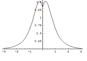
(a) $\phi_{\omega,Z}$: $\omega=-3$, $Z=-2$.

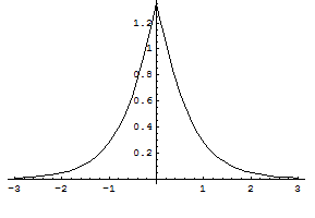
(b) $\phi_{\omega,Z}$: $\omega=-3$, $Z=2$.

Figure 1: The peak solutions $\phi_{\omega,Z}$ for $Z<0$ and $Z>0$.

4 Spectral properties

This section is dedicated to the study of the spectral properties of the operators associated to the second variation of the action functional $S_{\omega,Z}=E-\omega Q$ at the profile $\phi_{\omega}$ defined in (4). We note initially that $\phi_{\omega}$ is a critical point of $S_{\omega,Z}$. Next, we determine $S^{\prime\prime}_{\omega,Z}(\phi_{\omega})$. It consider $u,v\in H^{1}(\mathbb{R})$ such that $u=u_{1}+iu_{2},\,\,v=v_{1}+iv_{2}$. Then, we get

$$\begin{split}&S_{\omega,Z}^{\prime\prime}(\phi_{\omega})(u,v)=\int\limits_{\mathbb{R}}u^{\prime}_{1}v^{\prime}_{1}dx-\int\limits_{\mathbb{R}}u_{1}v_{1}(\omega+3\lambda_{1}\phi^{2}_{\omega}+5\lambda_{2}\phi^{4}_{\omega})dx-Zu_{1}(0)v_{1}(0)\\ &+\int\limits_{\mathbb{R}}u^{\prime}_{2}v^{\prime}_{2}dx-\int\limits_{\mathbb{R}}u_{2}v_{2}(\omega+\lambda_{1}\phi^{2}_{\omega}+\lambda_{2}\phi^{4}_{\omega})dx-\gamma u_{2}(0)v_{2}(0).\end{split}$$

Therefore, $S_{\omega,Z}^{\prime\prime}(\phi_{\omega})(u,v)$ can be formally rewritten as

$$S_{\omega,Z}^{\prime\prime}(\phi_{\omega})(u,v)=B_{1,Z}(u_{1},v_{1})+B_{2,Z}(u_{2},v_{2}),$$ (32)

where

$$\begin{split}&B_{1,Z}(f,g)=\int\limits_{\mathbb{R}}f^{\prime}g^{\prime}dx-\int\limits_{\mathbb{R}}fg(\omega+3\lambda_{1}\phi^{2}_{\omega}+5\lambda_{2}\phi^{4}_{\omega})dx-Zf(0)g(0),\\ &B_{2,Z}(f,g)=\int\limits_{\mathbb{R}}f^{\prime}g^{\prime}dx+\int\limits_{\mathbb{R}}fg(\omega+\lambda_{1}\phi^{2}_{\omega}+\lambda_{2}\phi^{4}_{\omega})dx-Zf(0)g(0),\end{split}$$ (33)

and $D(B_{j,Z})=H^{1}(\mathbb{R})\times H^{1}(\mathbb{R})$, $j\in\{1,2\}$. Note that the forms $B_{j,Z}$, $j\in\{1,2\},$ are bilinear bounded from below and closed. Therefore, by the First Representation Theorem (see [39, Chapter VI, Section 2.1]), they define operators $\mathcal{L}_{1,Z}$ and $\mathcal{L}_{2,Z}$ such that for $j\in\{1,2\}$

$$\left\{\begin{split}&D(\mathcal{L}^{\gamma}_{j})=\{v\in H^{1}(\mathbb{R}):\exists w\in L^{2}(\mathbb{R})\;s.t.\;\forall z\in H^{1}(\mathbb{R}),\;B_{j,Z}(v,z)=(w,z)\},\\ &\mathcal{L}_{j,Z}v=w.\end{split}\right.$$ (34)

In the following theorem we describe operators $\mathcal{L}_{1,Z}$ and $\mathcal{L}_{2,Z}$ in more explicit form. The proof of this theorem follows the same lines as in Le Coz et al. [23].

Theorem 6.

The operators $\mathcal{L}_{1,Z}$ and $\mathcal{L}_{2,Z}$ determined in (34) are given by

$$\begin{split}\mathcal{L}_{1,Z}=-\frac{d^{2}}{dx^{2}}-\omega-3\lambda_{1}\phi^{2}_{\omega}-5\lambda_{2}\phi^{4}_{\omega},\quad\mathcal{L}_{2,Z}=-\frac{d^{2}}{dx^{2}}-\omega-\lambda_{1}\phi^{2}_{\omega}-\lambda_{2}\phi^{4}_{\omega}\end{split}$$ (35)

on the domain $D_{Z}:=D\left({\cal L}_{i,Z}\right)=\left\{g\in H^{1}(\mathbb{R})\cap H^{2}(\mathbb{R}-\left\{0\right\})|g^{\prime}(0+)-g^{\prime}(0-)=-Zg(0)\right\}$.

Next, we proceed with the more delicate part of our theory, it which is associated to finding the Morse index of the self-adjoint operators ${\cal L}_{1,Z}$ and ${\cal L}_{2,Z}$ defined in Theorem 6. Here we will consider the parameters $\lambda_{1},\lambda_{2}$, $\omega$ and $Z$ such that satisfy the relations in Theorem 5. For finding this number we will use perturbation theory and we will follow the ideas in Le Coz et.al [23]. We also give an alternative approach based in the extension theory for symmetric operators of von Neumman and Krein established recently by Angulo&Goloshchapova ([13], [14]) for finding this index at least in the case $Z>0$ (see Appendix below).

Theorem 7.

Spectral properties of ${\cal L}_{2,Z}$. For $\omega<0$ and $Z$ satisfying $\omega+Z^{2}/4<0$, the self-adjoint linear operator ${\cal L}_{2,Z}:D_{Z}\rightarrow L^{2}(\mathbb{R})$ given in (35) has zero as a simple eigenvalue and $\phi_{\omega,Z}$ as its corresponding positive eigenfunction. The rest of the spectrum is positive and away from zero. Additionally, $\sigma_{ess}({\cal L}_{2,Z})=[-\omega,\infty)$.

Proof.

From (3) follows ${\cal L}_{2,Z}(\phi_{\omega,Z})=0$. Thus, since $\phi_{\omega,Z}>0$ we obtain from the Sturm-Liouville oscillation theory extended to operators with point interaction in Angulo&Goloshchapova [13, 14] that zero is a simple isolated eigenvalue, the remains of the spectrum is contained in $[\delta,+\infty)$ for $\delta>0$. Moreover, from Weyl’s theorem (see Reed&Simon [49]) we obtain the affirmation on the essential spectrum. ∎

Now, we study the kernel of ${\cal L}_{1,Z}$ for $Z\neq 0$.

Lemma 2.

For $Z\neq 0$ and $\lambda_{1},\lambda_{2}$ satisfying the conditions in Theorem 5, the kernel of ${\cal L}_{1,Z}$ is trivial.

Proof.

Let $v\in Ker({\cal L}_{1,Z})$, then we have

$$\left\{\begin{aligned} &{\cal L}_{1,Z}v(x)=0,\hskip 14.22636ptx>0.\\ &v\in L^{2}(0,\infty).\end{aligned}\right.$$ (36)

Now, since the linear problem (36) has dimension one (see [20]) and $\phi_{\omega}^{\prime}$ satisfies (36) then there exists $\alpha\in\mathbb{R}$ such that $v(x)=\alpha_{0}\phi^{\prime}_{\omega}(x)$, for all $x>0$. A similar argument shows $v(x)=\beta\phi^{\prime}_{\omega}(x)$, for $x<0$, with $\beta\in\mathbb{R}$. Next, from the continuity of $v$ and the parity of the function $\phi_{\omega}$, we deduce that $\alpha_{0}=-\beta$ and then we can rewrite $v$ as

$$v(x)=\begin{cases}\alpha_{0}\phi^{\prime}_{\omega}(x),&\text{if}\hskip 8.5359ptx\geq 0,\\ -\alpha_{0}\phi^{\prime}_{\omega}(x)&\text{if}\hskip 8.5359ptx<0.\end{cases}$$ (37)

Since $v\in{\cal D}({\cal L}_{1,Z})$ follows from (37)

$$v^{\prime}(0+)-v^{\prime}(0-)=\alpha_{0}\phi_{\omega}^{\prime\prime}(0+)+\alpha_{0}\phi_{\omega}^{\prime\prime}(0-)=-Z\alpha_{0}\phi_{\omega}^{\prime}(0+).$$ (38)

Now, we argue by contradiction. If $\alpha_{0}\neq 0$, from (25b) and (38), we obtain that $\phi_{\omega}^{\prime\prime}(0+)=-Z/2\phi_{\omega}^{\prime}(0+)$. Multiplying equation (25b) by $g^{\prime}$ and integrating on the interval $(0,R)$, we get

$$-\frac{1}{2}(g^{\prime}(R))^{2}+\frac{1}{2}(g^{\prime}(0+))^{2}-F(g(R))+F(g(0+))=0,$$ (39)

where $F(s)=\omega s^{2}/2+\lambda_{1}s^{4}/4+\lambda_{2}s^{6}/6$, by doing $R\rightarrow\infty$ and from (25d), we obtain

$$\frac{1}{2}(g^{\prime}(0+))^{2}+F(g(0+))=0.$$ (40)

Now, since $\phi_{\omega}$ satisfies equation (25b) then from (40), we infer that $\frac{1}{2}(\phi_{\omega}^{\prime}(0+))^{2}=-F(\phi_{\omega}(0))$. In addition, since $\phi_{\omega}$ is an even function, we obtain that $\phi_{\omega}^{\prime}(0+)=\frac{-Z}{2}\phi_{\omega}(0)$. Therefore, we deduce that $\phi_{\omega}(0)>0$ is a zero of the following function

$$P(s)=\frac{Z^{2}}{8}s^{2}+\omega\frac{s^{2}}{2}+\lambda_{1}\frac{s^{4}}{4}+\lambda_{2}\frac{s^{6}}{6}.$$ (41)

On the other hand, from equation (25b), we have that

$$\lim_{x\rightarrow 0+}\phi_{\omega}^{\prime\prime}(x)=\phi_{\omega}^{\prime\prime}(0+)=-\omega\phi_{\omega}(0)-\lambda_{1}\phi^{3}_{\omega}(0)-\lambda_{2}\phi^{5}_{\omega}(0),$$ (42)

and since $\phi_{\omega}^{\prime\prime}(0+)=\frac{Z^{2}}{4}\phi_{\omega}(0)$, we deduce that $\phi_{\omega}(0)$ is a positive zero of the function

$$R(s)=\frac{Z^{2}}{4}s+\omega s+\lambda_{1}s^{3}+\lambda_{2}s^{5}.$$ (43)

Now, since $s_{0}=\phi_{\omega}(0)$ is a zero of both (41) and (43), after some algebraic manipulations, we deduce that

$$s_{0}^{2}=-\frac{3\lambda_{1}}{4\lambda_{2}},$$ (44)

and so we get immediately a contradiction when $\lambda_{1},\lambda_{2}>0$. Now, in the case $\lambda_{1}>0$ and $\lambda_{2}<0$, we obtain from (4)-(24) the relation $\phi^{2}_{\omega}(0)\leqq\phi^{2}(0)$ and therefore

$$-\frac{3\lambda_{1}}{4\lambda_{2}}\leqq-\frac{3\lambda_{1}}{4\lambda_{2}}\frac{1}{1+\frac{4}{\lambda_{1}}\sqrt{\frac{\lambda^{2}_{1}}{16}-\omega\frac{\lambda_{2}}{3}}},$$

it which is a contradiction. Therefore, we conclude that $\alpha_{0}=0$ and then $v\equiv 0$. It finished the proof. ∎

Remark 5.

Our restrictions about the sign of the parameters $\lambda_{1},\lambda_{2}$ are evidenced by the identity (44). Thus for the case $\lambda_{1}<0$ and $\lambda_{2}>0$ is not clear for us that the statement in Lemma 2 is true.

Now, for starting our study based in perturbation theory, we establish the spectral structure of our “limiting” operator associated to ${\cal L}_{1,Z}$ when $Z\neq 0$.

Theorem 8.

Spectral properties of ${\cal L}_{1,0}$. For $\omega<0$, we consider the self-adjoint linear operator ${\cal L}_{1,0}:H^{2}(\mathbb{R})\rightarrow L^{2}(\mathbb{R})$ given by

$${\cal L}_{1,0}=-\frac{d^{2}}{dx^{2}}-\omega-3\lambda_{1}\phi^{2}_{\omega,0}-5\lambda_{2}\phi^{4}_{\omega,0}$$

with $\phi_{\omega,0}$ being the profile $\phi_{\omega,Z}$ in the case $Z=0$. Then, ${\cal L}_{1,0}$ has a unique negative simple eigenvalue $-\lambda$, with $\lambda>0$. Zero is a simple eigenvalue with eigenfunction $\phi^{\prime}_{\omega,0}$. The rest of the spectrum is away from zero. Additionally, $\sigma_{ess}({\cal L}_{1,0})=[-\omega,\infty)$.

Proof.

Since ${\cal L}_{1,0}(\phi^{\prime}_{\omega,0})=0$ and $\phi^{\prime}_{\omega,0}$ has a unique zero in $x=0$, we obtain immediately from the classical Sturm-Liouville oscillation theory (see Berezin&Shubin [20]) the theorem. ∎

Now, we show that the family of operators ${\cal L}_{1,Z}$ depends analytically of the variable $Z$, with $Z$ satisfying the conditions in Theorem 5.

Lemma 3.

As a function of the variable $Z$, $\left\{{\cal L}_{1,Z}\right\}$ is a real analytic family of self-adjoint operators of type (B) in the sense of Kato.

Proof.

From the theorem VII-4.2 in Kato [39] and Reed and Simon [49], it is enough to show that the bilinear forms given in (33) are real analytic of type (B), namely

1. The domain $D(B_{1,Z})$ of the forms ${B}_{1,Z}$ is independent of the parameter $Z$. In our case, $D({B}_{1,Z})=H^{1}(\mathbb{R})$ for $Z$ satisfying the conditions in Theorem 5.

2. For each $Z$, ${B}_{1,Z}$ is closed and bounded from below.

3. Since $\phi_{\omega,Z}$ and $R$ given in (4) and (29), respectively, are analytic functions then $\phi_{\omega,Z}$ is an analytic function of $Z$. Thus, for each $v\in H^{1}(\mathbb{R})$ the function $Z\rightarrow{B}_{1,Z}(v,v)$ is analytic.

It finishes the proof. ∎

Next, we use the Kato-Rellich theorem to prove some specific properties of the second eigenvalue and eigenfunction of the operator ${\cal L}_{1,Z}$. Namely,

Lemma 4.

There exist $Z_{0}>0$ and analytic functions $\Pi_{2}:(-Z_{0},Z_{0})\rightarrow\mathbb{R}$, $\Omega_{2}:(-Z_{0},Z_{0})\rightarrow L^{2}(\mathbb{R})$, such that

1. For each $Z\in(-Z_{0},Z_{0})$, $\Pi_{2}(Z)$ is the second eigenvalue of ${\cal L}_{1,Z}$, which is simple and $\Omega_{2}(Z)$ its corresponding eigenfunction.

2. $\Pi_{2}(0)=0$ and $\Omega_{2}(0)=\phi^{\prime}$, with $\phi=\phi_{\omega,0}$ given in (24).

3. $Z_{0}$ can be chosen small enough such that the spectrum of ${\cal L}_{1,Z}$ with $Z\in(-Z_{0},Z_{0})$ is greater than $0$ except by the first $2$ eigenvalues.

Proof.

The proof is standard. Indeed, there is a positive $M$ such that $\sigma\left({\cal L}_{1,Z}\right)\cap(-\infty,-M)=\emptyset$ for $Z\in[-a,a]$, $a$ small enough. From Theorem 8, defining $\lambda_{1,0}=-\lambda$ and $\lambda_{2,0}=0$, we can separate the spectrum $\sigma\left({\cal L}_{1,0}\right)$ of ${\cal L}_{1,0}$ into two parts $\sigma_{0}=\{-\lambda,0\}$ and $\sigma_{1}=[-\omega,\infty)$ by a simple closed curve $\Gamma\subset\rho\left({\cal L}_{1,0}\right)$ such that $\sigma_{0}\subset\text{Int}(\Gamma)$ and $\sigma_{1}$ in its exterior. Here, $\text{Int}(\Gamma)$ denotes the interior of $\Gamma$. From Lemma 3 we can see that ${\cal L}_{1,Z}$ converges to ${\cal L}_{1,0}$ as $Z\to 0$ in the generalized sense (see Kato [39]). So, from Theorem IV-3.16 in Kato [39], we have that $\Gamma\subset\rho\left({\cal L}_{1,Z}\right)$ for $Z\in(-\epsilon_{1},\epsilon_{1})$, $\epsilon_{1}$ small enough, and $\sigma\left({\cal L}_{1,Z}\right)$ is also separated by $\Gamma$ into two parts such that the part of $\sigma\left({\cal L}_{1,Z}\right)$ inside $\Gamma$ consists of a finite set of eigenvalues with total algebraic multiplicity $2$.

Now, for $i=1,2$, and $\gamma>0$ small enough we define the circles $\Gamma_{i}=\{z\in\mathbb{C}:|z-\lambda_{i,0}|=\gamma\}$, such that $\Gamma_{1}\cap\Gamma_{2}=\emptyset$ and $\Gamma_{i}$ is in the interior of $\Gamma$. Thus from the nondegeneracy of the eigenvalues $-\lambda_{i,0}$, we obtain that there exists $0<Z_{1}<\epsilon_{1}$ such that for $Z\in(-Z_{1},Z_{1})$, $\sigma\left({\cal L}_{1,Z}\right)\cap\text{Int}(\Gamma_{i})=\left\{\lambda_{i,Z}\right\}$, where $\lambda_{i,Z}$ are simple eigenvalues for ${\cal L}_{1,Z}$, furthermore, $\lambda_{i,Z}\to\lambda_{i,0}$, as $Z\to 0$. Applying the Kato-Rellich’s theorem (Theorem XII.8 in [49]) for each one of the simple eigenvalues $\lambda_{i,0}$, $i=1,2.$, we obtain the existence of a positive $Z_{0}<Z_{1}$, and two analytic functions $\Pi_{2},\Omega_{2}$ defined on the intervals $(-Z_{0},Z_{0})$ satisfying the items (i),(ii) and (iii) of the theorem. It finishes the proof. ∎

Now, we proceed to count the number of negative eigenvalues of the operator ${\cal L}_{1,Z}$. First of all, we do this for $Z$ small.

Lemma 5.

There exists $0<r<Z_{0}$ such that $\Pi_{2}(Z)<0$, for any $Z\in(-r,0)$ and $\Pi_{2}(Z)>0$ for any $Z\in(0,r)$. Therefore, for $Z$ negative and small ${\cal L}_{1,Z}$ has exactly two negative eigenvalues and for $Z$ positive and small ${\cal L}_{1,Z}$ has exactly one negative eigenvalue.

Proof: By application of Taylor theorem around $Z=0$, the functions $\Pi_{2}$ and $\Omega_{2}$ in Lemma 4 can be written as

$$\Pi_{2}(Z) =\beta Z+O\left(Z^{2}\right),$$ (45)

$$\Omega_{2}(Z) =\phi^{\prime}_{\omega,0}+Z\psi_{0}+O\left(Z^{2}\right),$$

where $\phi^{\prime}_{\omega,0}=\frac{d}{dx}\phi_{\omega,0}$, $\beta\in\mathbb{R}$, ($\beta=\Pi_{2}^{\prime}(0)$) and $\psi_{0}\in L^{2}(\mathbb{R})$ $(\psi_{0}=\Omega_{2}^{\prime}(0))$. To obtain our result, it is enough to show that $\beta>0$ or equivalently that $\Pi_{2}(Z)$ is an increasing function of the variable $Z$ around $Z=0$. Since the function $Z\rightarrow\phi_{\omega,Z}$ is analytic, then for $Z$ close to zero, we have that

$$\phi_{\omega,Z}=\phi_{\omega,0}+Z\chi_{0}+O\left(Z^{2}\right).$$ (46)

where

$$\chi_{0}=\left.\frac{d}{dZ}\phi_{\omega,Z}\right|_{Z=0}.$$ (47)

Now, from the equation (3), we have that for all $\psi\in H^{1}(\mathbb{R})$,

$$\left\langle-\phi^{\prime\prime}_{\omega,Z}-\omega\phi_{\omega,Z}-\lambda_{1}\phi^{3}_{\omega,Z}--\lambda_{2}\phi^{5}_{\omega,Z},\psi\right\rangle=Z\phi_{\omega,Z}(0)\psi(0).$$ (48)

Taking derivative with respect to the variable $Z$ in (48) and evaluating in $Z=0$, we get that

$$\left\langle{\cal L}_{1,0}\chi_{0},\psi\right\rangle=\phi_{\omega,0}(0)\psi(0).$$ (49)

In order to obtain $\beta$ as a function of the variable $Z$. We compute the quantity $\left\langle{\cal L}_{1,Z}\Omega_{2}(Z),\phi^{\prime}_{\omega,0}\right\rangle$ in two different ways

1. Since ${\cal L}_{1,Z}\Omega_{2}(Z)=\Pi_{2}(Z)\Omega_{2}(Z)$, then from (45)

   $$\left\langle{\cal L}_{1,Z}\Omega_{2}(Z),\phi^{\prime}_{\omega,0}\right\rangle=\beta Z||\phi^{\prime}_{\omega,0}||^{2}+O\left(Z^{2}\right).$$ (50)

2. Since ${\cal L}_{1,Z}$ is selfadjoint, then $\left\langle{\cal L}_{1,Z}\Omega_{2}(Z),\phi^{\prime}_{\omega,0}\right\rangle=\left\langle\Omega_{2}(Z),{\cal L}_{1,Z}\phi^{\prime}_{\omega,0}\right\rangle$. Now, since ${\cal L}_{1,0}\phi^{\prime}_{\omega,0}=0$, it follows from (47) that

   $${\cal L}_{1,Z}\phi^{\prime}_{\omega,0} ={\cal L}_{1,0}\phi^{\prime}_{\omega,0}+\left[f^{\prime}\left(\phi_{\omega,0}\right)-f^{\prime}\left(\phi_{\omega,Z}\right)\right]\phi^{\prime}_{\omega,0}$$ (51)

   $$=\left[f^{\prime}\left(\phi_{\omega,0}\right)-f^{\prime}\left(\phi_{\omega,0}+Z\chi_{0}+O(Z^{2})\right)\right]\phi^{\prime}_{\omega,0}$$

   $$=-f^{\prime\prime}\left(\phi_{\omega,0}\right)Z\chi_{0}\phi^{\prime}_{\omega,0}+O\left(Z^{2}\right)$$

   where $f(x)=\lambda_{1}x^{3}+\lambda_{2}x^{5}$. Thus, from (45) and (51), we obtain that

   $$\left\langle{\cal L}_{1,Z}\Omega_{2}(Z),\phi^{\prime}_{\omega,0}\right\rangle =-Z\left\langle\phi^{\prime}_{\omega,0},f^{\prime\prime}\left(\phi_{\omega,0}\right)\chi_{0}\phi^{\prime}_{\omega,0}\right\rangle+O(Z^{2}).$$ (52)

   On the other hand, by direct computation, we see that

   $${\cal L}_{1,0}(-\omega\phi_{\omega,0}-f\left(\phi_{\omega,0}\right))=f^{\prime\prime}(\phi_{\omega,0})[\phi^{\prime}_{\omega,0}]^{2}.$$ (53)

   Using (49), (52), (53) and that $\phi_{\omega,0}$ satisfies equation (20), we obtain that

   $$\left\langle{\cal L}_{1,Z}\Omega_{2}(Z),\phi^{\prime}_{\omega,0}\right\rangle =-Z\left\langle\chi_{0},f^{\prime\prime}(\phi_{\omega,0})[\phi^{\prime}_{\omega,0}]^{2}\right\rangle+O\left(Z^{2}\right)$$ (54)

   $$=-Z\left\langle-{\cal L}_{1,0}\chi_{0},-\omega\phi_{\omega,0}-f\left(\phi_{\omega,0}\right)\right\rangle+O\left(Z^{2}\right)$$

   $$=-Z\phi_{\omega,0}(0)(-\omega\phi_{\omega,0}(0)-f(\phi_{\omega,0}(0)))+O\left(Z^{2}\right)$$

   $$=-Z\phi_{\omega,0}(0)(\phi^{\prime\prime}_{\omega,0}(0))+O\left(Z^{2}\right).$$

Finally, from (50) and (54), we conclude that

$$\beta=-\frac{\phi_{\omega,0}(0)\phi^{\prime\prime}_{\omega,0}(0)}{||\phi^{\prime}_{\omega,0}||^{2}}+O(Z).$$ (55)

Hence $\Pi_{2}^{\prime}(0)=\beta>0$ for $Z$ small. This completes the proof of the lemma.  

Now, we are in position for counting the number of negative eigenvalues of $\mathcal{L}_{i,Z}$ for every $Z$ admissible. By using a classical continuation argument based on the Riesz-projection and denoting the number of negatives eigenvalues of $\mathcal{L}_{i,Z}$ by $n(\mathcal{L}_{i,Z})$, we have the following characterization.

Theorem 9.

Let $\lambda_{1},\lambda_{2}$, and $\omega,Z$ satisfy the conditions in Theorem 5. Then,

1. For the case of being $Z$ negative, $n\left({\cal L}_{1,Z}\right)=2$.

2. For the case of being $Z$ positive, $n\left({\cal L}_{1,Z}\right)=1$.

Proof: The proof is based in Lemma 2 above and the ideas in Le Coz et al. [23]

We finish this section with the following information about the second eigenfunction $\Omega_{2}(Z)$ of the operator ${\cal L}_{1,Z}$ obtained in Lemma 4.

Proposition 1.

The eigenfunction $\Omega_{2}(Z)$ of the linear operator ${\cal L}_{1,Z}$ associated to the second eigenvalue $\Pi_{2}(Z)$ obtained in Lemma 4 can be extended for all $Z$ admissible. Moreover, $\Omega_{2}(Z)$ is an odd function.

Proof: The proof follows the same ideas as in [23].

5 Convexity condition

In this section, we study the behavior of the function $\omega\rightarrow-\partial_{\omega}||\phi_{\omega,Z}||^{2}$ with $\phi_{\omega,Z}$ given in (4). Due to the complexity of the formulas appearing in our calculations we need to use the mathematical software Mathematica. We divide our analysis in the two cases:

1. $\lambda_{1}=\lambda_{2}=1$ (for the general case, $\lambda_{1},\lambda_{2}>0$, similar analysis can be done): we have initially from (31) that

   $$\int_{-\infty}^{\infty}\phi_{\omega,Z}^{2}(x)dx =\int_{-\infty}^{\infty}\frac{1}{\alpha(\omega)+\beta(\omega)\text{cosh}(2\sqrt{-\omega}(|x|+b))}dx,$$ (56)

   $$=\frac{1}{\sqrt{-\omega}}\int_{2\sqrt{-\omega}b}^{\infty}\frac{1}{\alpha(\omega)+\beta(\omega)\text{cosh}(u)}du,$$

   with $\alpha(\omega)=\frac{-1}{4\omega}$, $\beta(\omega)=\frac{\sqrt{9-48\omega}}{-12\omega}$, $b=R_{\omega}^{-1}\left(\frac{Z}{2\sqrt{-\omega}}\right)$ and $R_{\omega}$ given by

   $$R_{\omega}(b)=\frac{\beta(\omega)\text{sinh}(2\sqrt{-\omega}b)}{\alpha(\omega)+\beta(\omega)\text{cosh}(2\sqrt{-\omega}b)}.$$ (57)

   By setting $\gamma(\omega)=\frac{\sqrt{3}}{\sqrt{3-16\omega}}$, we rewrite (56) in the following form

   $$\int_{-\infty}^{\infty}\phi_{\omega,Z}^{2}(x)dx =\frac{1}{\beta(\omega)\sqrt{-\omega}}\int_{2\sqrt{-\omega}b}^{\infty}\frac{1}{\gamma(\omega)+\text{cosh}(u)}du$$ (58)

   $$=-2\sqrt{3}\text{ }\text{arctan }\left(\frac{\sqrt{3}-\sqrt{3-16\omega}}{4\sqrt{-\omega}}\text{ }\text{tanh}\left(\frac{u}{2}\right)\right)\Biggr{|}_{u=2\sqrt{-\omega}b}^{u=\infty},$$

   that is

   $$||\phi_{\omega,Z}||^{2}=-2\sqrt{3}\left[\text{arctan}\left(\theta(\omega)\right)-\text{arctan}\left(\theta(\omega)\text{ }\text{tanh}(\sqrt{-\omega}b)\right)\right],$$ (59)

   with $\theta(\omega)=\frac{\sqrt{3}-\sqrt{3-16\omega}}{4\sqrt{-\omega}}$. Now, we will obtain a formula to compute $\frac{db}{d\omega}$. From the relation (57) and setting

   $$H(\omega,b)=2\sqrt{-\omega}R_{\omega}(b),$$ (60)

   we deduce from (28)-(29) that $H(\omega,b)=Z$. Furthermore, since $\partial_{b}H>0$, then from the chain rule we deduce that

   $$\frac{db}{d\omega}=-\frac{\partial_{\omega}H}{\partial_{b}H},$$

   therefore, using (57) and (60), we conclude that

   $$\frac{db}{d\omega}(\omega,b)=\frac{4\sqrt{3}\sqrt{-\omega}h(\omega)b\text{ }\text{cosh}(s(\omega)b)+2\sqrt{3}(3-32\omega)\text{sinh}(s(\omega)b)+t(\omega)}{8(-\omega)^{\frac{3}{2}}\sqrt{h(\omega)}(h(\omega)+\sqrt{3}\sqrt{h(\omega)}\text{cosh}(s(\omega)b))},$$ (61)

   where $t(\omega)=h(\omega)^{\frac{3}{2}}(2s(\omega)b+\text{sinh}(2s(\omega)b))$, $h(\omega)=3-16\omega$ and $s(\omega)=2\sqrt{-\omega}$. Finally, from (59) we obtain that

   $$\frac{1}{2\sqrt{3}}\partial_{\omega}||\phi_{\omega,Z}||^{2}=\frac{3-\sqrt{3h(\omega)}}{u(\omega)\sqrt{-\omega h(\omega)}}+\\ \frac{\text{sech}^{2}(\sqrt{-\omega}b)\left[-2bu(\omega)\sqrt{-\omega}+\text{sinh}(2\sqrt{-\omega}b)(3-\sqrt{3h(\omega)})+4u(\omega)b^{\prime}(\omega)(-\omega)^{\frac{3}{2}}\right]}{2\sqrt{-\omega h(\omega)}(8\omega+\text{tanh}^{2}(\sqrt{-\omega}b)(-3+8\omega+\sqrt{3h(\omega)}))},$$ (62)

   where $u(\omega)=h(\omega)+\sqrt{3h(\omega)}$.

   Next, by using the computational software program Mathematica, we study the behavior of the functions $(\omega,Z)\rightarrow-||\phi_{\omega,Z}||^{2}$ and $(\omega,Z)\rightarrow-\partial_{\omega}||\phi_{\omega,Z}||^{2}$ given in (59) and (62), respectively. After some two-dimensional plots by fixing one interval for $\omega$ and by choosing specific values for $Z$ we find the existence of a unique threshold value $Z^{*}$ of $Z$ such that the function $(\omega,Z)\rightarrow-\partial_{\omega}||\phi_{\omega,Z}||^{2}$ changes of signal. We also study the derivate-function $(\omega,Z)\rightarrow-\partial_{\omega}||\phi_{\omega,Z}||^{2}$ via a three-dimensional surface and we also saw the possible location of $Z^{*}$.

   Hence, after a delicated numerical study for determining the threshold value of $Z$ associated to the mapping $\omega\to-\partial_{\omega}||\phi_{\omega,Z}||^{2}$ we can establish the following result.

   Theorem 10.

   Let $\lambda_{1}=\lambda_{2}=1$ in (4) and it consider $\omega,Z$ such that $\omega+\frac{Z^{2}}{4}<0$. Then there is a threshold value $Z^{*}$, $Z^{*}\approx-0.8660254$, such that the function $\omega\rightarrow-||\phi_{\omega,Z}||^{2}$ satisfies the following properties:

   $$\begin{cases}-\partial_{\omega}||\phi_{\omega,Z}||^{2}>0,&\text{if $Z>Z^{*}$},\\ -\partial_{\omega}||\phi_{\omega,Z}||^{2}<0,&\text{if $Z<Z^{*}$},\end{cases}$$ (63)

   Next, we give some numerical justification which led us to establish the above result. Thus, by instance, for $\omega\in(-6,-1)$, $Z=-0.86$, and $\omega\in(-6,-1)$, $Z=-0.9$, in Figure 2, (a)-(b), respectively, we see that there is a drastic change in the growth of the function $\omega\rightarrow-||\phi_{\omega,Z}||^{2}$ for some value of the parameter $Z\in(-0.9,-0.8)$. In the same way, Figure 3 (three dimensional) showed us a remarkable change on the behavior of the function $\omega\rightarrow-\partial_{\omega}||\phi_{\omega,Z}||^{2}$. For considering $\omega\in(-50,-2)$, $Z\in(-0.9,-0.8)$ and $Z\in(-0.8,-0.7)$, the three dimensional plot was more conclusive about the existence of a threshold value of $Z^{*}$. Now, for fixing $Z=-0.86602$ and $Z=-0.86603$ (see Figure 4), we improved our numerical localization for $Z^{*}$.

   

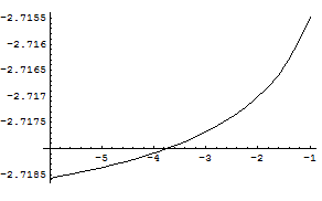
   (a) $\omega\in(-6,-1)$, $Z=-0.86$.

   

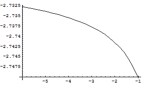
   (b) $\omega\in(-6,-1)$, $Z=-0.9$.

   Figure 2: Function $\omega\to-||\phi_{\omega,Z}||^{2}$ for specific values of $Z$.

   

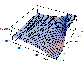
   (a) $\omega\in(-50,-2)$, $Z\in(-0.9,-0.8)$.

   

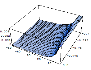
   (b) $\omega\in(-50,-2)$, $Z\in(-0.8,-0.7)$.

   Figure 3: Function $(\omega,Z)\to-\partial_{\omega}||\phi_{\omega,Z}||^{2}$, $\omega\in(-50,-2)$, $Z\in(-0.9,-0.8)$ and $Z\in(-0.8,-0.7)$

   

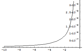
   (a) $\omega\in(-10,-0.8)$, $Z=-0.86602$.

   

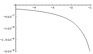
   (b) $\omega\in(-5,-1)$, $Z=-0.86603$.

   Figure 4: Function $\omega\to-\partial_{\omega}||\phi_{\omega,Z}||^{2}$ for specific values of $Z$.

   Remark 6.

   From our numerical study, $Z^{*}$ in Theorem 10 is the only critical point of the mapping $\omega\to-||\phi_{\omega,Z}||^{2}$.

2. $\lambda_{1}>0$ and $\lambda_{2}<0$: since $Z$ and $\omega$ belong to a bounded interval, our numerical simulations are more accurate. Indeed, Figures 5 and 6 show the mapping $\omega\to-||\phi_{\omega,Z}||^{2}$ for specific values of the parameters $\lambda_{1}>0$, $\lambda_{2}<0$, $Z$, and $\omega\in(-\frac{3}{4},-\frac{1}{4})$. These simulation showed us clearly that the mapping $\omega\to-\partial_{\omega}||\phi_{\omega,Z}||^{2}$ is strictly positive.

   

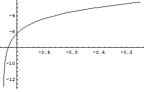
   (a) $\lambda_{1}=2$, $\lambda_{2}=-1$, $Z=-1$.

   

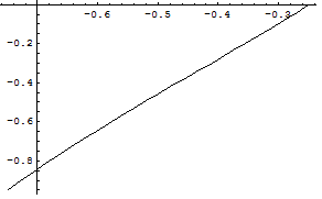
   (b) $\lambda_{1}=2$, $\lambda_{2}=-1$, $Z=1$.

   Figure 5: The function $\omega\to-||\phi_{\omega,Z}||^{2}$, for $\omega\in(-\frac{3}{4},-\frac{1}{4})$ and $Z=\pm 1$.

   

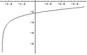
   (a) $\lambda_{1}=4$, $\lambda_{2}=-2$, $Z=-1$.

   

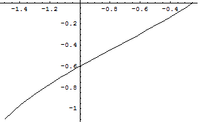
   (b) $\lambda_{1}=4$, $\lambda_{2}=-2$, $Z=1$.

   Figure 6: The function $\omega\to-||\phi_{\omega,Z}||^{2}$, for $\omega\in(-\frac{3}{2},-\frac{1}{4})$ and $Z=\pm 1$.

   Therefore, from a detailed numerical study we can conclude the following result.

   Theorem 11.

   Let $\lambda_{1}>0,\lambda_{2}<0$ in (4) and it consider $\omega,Z$ such that $\frac{Z^{2}}{4}<-\omega<-\frac{3\lambda_{1}^{2}}{16\lambda_{2}}$. Then, $-\partial_{\omega}||\phi_{\omega,Z}||^{2}>0$.

6 Stability Theory

Our stability results, Theorem 1 and Theorem 2, it will based in the Instability Theorem and Stability Theorem in [35]. Thus, by the sake of self-containdness we establish it.

Theorem 12.

Let $Z\neq 0$ fixed and

$$p_{Z}(\omega_{0})=\begin{cases}\begin{aligned} &1,\quad{\text{if}}\;\;-\partial_{\omega}\|\phi_{\omega,Z}\|^{2}>0,\;\;at\;\;\omega=\omega_{0},\\ &0,\quad{\text{if}}\;\;-\partial_{\omega}\|\phi_{\omega,Z}\|^{2}<0,\;\;at\;\;\omega=\omega_{0}.\end{aligned}\end{cases}$$

We denote $\mathcal{H}_{\omega_{0},Z}=S^{\prime\prime}_{\omega_{0},Z}(\phi_{\omega_{0},Z})$, so from the analysis in section 4 we have

$$\mathcal{H}_{\omega_{0},Z}=\begin{bmatrix}{\cal L}_{1,Z}&0\\ 0&{\cal L}_{2,Z}\end{bmatrix}.$$

Suppose that $Ker(L_{2,Z})=[\phi_{\omega_{0},Z}]$, ${\cal L}_{2,Z}\geq 0$, and $Ker({\cal L}_{1,Z})=\{0\}$. Then from [35] the following assertions hold:

• If $n(\mathcal{H}_{\omega_{0},Z})=p_{Z}(\omega_{0})$, then the standing wave $e^{-i\omega_{0}t}\phi_{\omega_{0},Z}$ is orbitally stable in $H^{1}(\mathbb{R})$.

• If $n(\mathcal{H}_{\omega_{0},Z})-p_{Z}(\omega_{0})$ is odd, then the standing wave $e^{-i\omega_{0}t}\phi_{\omega_{0},Z}$ is orbitally unstable in $H^{1}(\mathbb{R})$.

Analogous result holds for the case of changing the space $H^{1}(\mathbb{R})$ by $H_{even}^{1}(\mathbb{R})$.

Remark 7.

The instability criterium part set up above deserves some comments:

1. it is well known from [35] that when $n(\mathcal{H}_{\omega_{0},Z})-p_{Z}(\omega_{0})$ is odd, we obtain only spectral instability of $e^{i\omega t}\phi_{\omega_{0},Z}$. Now, for obtaining orbital instability due to Theorem 6.1 in [35], it is sufficient to show estimate (6.2) in [35] for the semigroup $e^{t\mathbf{A}_{\omega,Z}}$ generated by

   $$\mathbf{A}_{\omega,Z}=\left(\begin{array}[]{cc}0&\mathcal{L}_{2,Z}\\ -\mathcal{L}_{1,Z}&0\end{array}\right).$$

   For us, it is non-clear how to obtain that estimate (6.2).

2. In the particular case $n(\mathbf{H}_{\omega_{0},Z})=2$ (it which will happened for the case $Z<0$) we can to apply the results in Ohta [47, Corollary 3 and 4] for obtaining orbital instability part of the above theorem. We note that in this case the instability results are obtained without using one argument through linear instability.

3. For justifying in a general framework (namely, $n(\mathbf{H}_{\omega_{0},Z})=2$ no necessarily being true) orbital instability implications from a spectral instability result in the case of the model (1), we can use the approach established in [36, Theorem 2]. The key point of this method is to use that the mapping data-solution associated to model (1) is at least of class $C^{2}$ (see Theorem 3 above). We note that the results in [36] have been applied successfully in the case of Schrödinger models on start graphs [11]-[12] and in [15]-[16] for models of KdV-type.

Proof.

$[$Theorem 1]

Let $\omega$ such that $\omega+\frac{Z^{2}}{4}<0$. From Theorems 7 and 2 we have for every $Z\neq 0$ that $Ker(L_{2,Z})=[\phi_{\omega,Z}]$, ${\cal L}_{2,Z}\geq 0$, and $Ker({\cal L}_{1,Z})=\{0\}$.

1. For $Z>0$ we have from Theorem 9 and Theorem 10 that $n(\mathcal{H}_{\omega,Z})=p_{Z}(\omega)$ Thus from Theorem 12 we have that $e^{-i\omega t}\phi_{\omega,Z}$ is orbitally stable in $H^{1}(\mathbb{R})$. We note that we have initially a “conditional stability” for the profile $\phi_{\omega,Z}$, because of, for $u_{0}\in U_{\eta}(\phi_{\omega,Z})$ we have that the solution $u(t)$ of (7) satisfies $u(t)\in U_{\epsilon}(\phi_{\omega,Z})$ for all $t\in(-T^{*},T^{*})$, where $T^{*}$ represents the maximal time of existence of the solution $u=u(t)$. But, as we will be shown below (Theorem 13), $T^{*}=+\infty$.

2. Let $Z\in(Z^{*},0)$. From Theorem 10 we have $p_{Z}(\omega)=1$. Then from Theorem 9 follows that $n(\mathcal{H}_{\omega,Z})-p_{Z}(\omega)=2-1=1$. Thus we obtain from Remark 7-$b)$ that $e^{-i\omega t}\phi_{\omega,Z}$ is orbitally unstable in $H^{1}(\mathbb{R})$. By Remark 7-$c)$ and Theorem 3, it nonlinear instability behavior can be deduced from a spectral instability result.

3. Let $Z\in(Z^{*},+\infty)$. From Proposition 1, the second eigenvalue of ${\cal L}_{1,Z}$ on $L^{2}(\mathbb{R})$ has associated an odd eigenfunction. So, such eigenvalue disappears when ${\cal L}_{1,Z}$ is restricted to the space $H^{2}_{even}(\mathbb{R})$ (we note that in this case ${\cal L}_{1,Z}:H^{2}_{even}(\mathbb{R})\to L^{2}_{even}(\mathbb{R})$). In addition, since $\phi_{\omega,Z}$ is an even function with $\left\langle{\cal L}_{1,Z}\phi_{\omega,Z},\phi_{\omega,Z}\right\rangle<0$, for all $Z\neq 0$, then the first eigenvalue of the operator ${\cal L}_{1,Z}$ is still present. In other words, we have that $n(\mathcal{H}_{\omega,Z}|_{H^{1}_{even}(\mathbb{R})})=1$. Therefore, from the persistence of the solution for (7) on the space $H^{1}_{even}(\mathbb{R})$ and $p_{Z}(\omega)=1$ we obtain, similarly as in item $a)$ above, that $e^{-i\omega t}\phi_{\omega,Z}$ is “conditionally stable” on $H^{1}_{even}(\mathbb{R})$. But, as we will be shown below (Theorem 13), the solution really is global.

4. Let $Z<Z^{*}$. Following a similar analysis as in item $c)$ above, we can see that $n(\mathcal{H}_{\omega,Z}|_{H^{1}_{even}(\mathbb{R})})=1$. Since $p_{Z}(\omega)=0$, follows from Remark 7-$a)$ that the profile $e^{-i\omega t}\phi_{\omega,Z}$ is spectrally unstable. Therefore, from Theorem 3 and Remark 7-$c)$ follow that $e^{-i\omega t}\phi_{\omega,Z}$ is nonlinearly unstable in $H^{1}_{even}(\mathbb{R})$ and so in $H^{1}(\mathbb{R})$.

∎

Proof.

$[$Theorem 2]

The proof is similar to that given for Theorem 1 above, by considering Theorem 3 (global existence for any initial data), Theorem 12, Remark 7 and Theorem 11. ∎

Remark 8.

As we do not have a global well posedness result of the Cauchy problem (7) for any initial data in the case $\lambda_{1},\lambda_{2}>0$, the orbital stability results given in the proof of Theorem 1 above are already valid just for the existence time of solution $u(t)$. However, if we combine the local well posedness result in Theorem 3 and our conditional stability result is possible to have the existence of global solutions of the Cauchy problem (7) for initial data close to the orbit $\Omega_{\phi_{\omega,Z}}=\{e^{i\theta}\phi_{\omega,Z}:\theta\in[0,2\pi]\}$.

Theorem 13.

(Global existence of solutions for (1) close to the orbit $\Omega_{\phi_{\omega,Z}}$)

Let $\lambda_{1},\lambda_{2}>0$. Then, all solutions $u=u(t)$ of equation (1) there is for all time, provided:

1. the initial data $u(0)=u_{0}\in H^{1}(\mathbb{R})$ is close to the orbit $\Omega_{\phi_{\omega,Z}}$ with $Z>0$.

2. the initial data $u(0)=u_{0}\in H_{even}^{1}(\mathbb{R})$ close to the orbit $\Omega_{\phi_{\omega,Z}}$ with $Z>Z^{*}$ .

Proof.

We will show that $u(t)$ is bounded in the $H^{1}(\mathbb{R})$-norm. Indeed, from the conditional stability result of the orbit $\Omega_{\phi_{\omega,Z}}$ ($Z>0$ and $Z>Z^{*}$) established initially in the proof of Theorem 1, we have that for $\epsilon>0$, there exists $\eta>0$ such that for some $s\in\mathbb{R}$

$$||u(t)-e^{-is}\phi_{\omega,Z}||_{1}\leq\epsilon,\text{ }\text{ }\text{ }\text{ }\forall t\in(-T^{*},T^{*}),$$ (64)

whenever the initial data $u(0)=u_{0}$ satisfies that $\inf_{s\in[0,2\pi]}||u_{0}-e^{-is}\phi_{\omega,Z}||_{1}<\eta$, with $T^{*}$ denoting the maximal time of existence of the solution $u=u(t)$ given by Theorem 3. Now, from the inequality (holds for all $s\in\mathbb{R}$ and $t\in(-T^{*},T^{*})$)

$$||u(t)||_{1}\leq||u(t)-e^{-is}\phi_{\omega,Z}||_{1}+||e^{-is}\phi_{\omega,Z}||_{1}<\epsilon+||\phi_{\omega,Z}||_{1},$$ (65)

with $\inf_{s\in[0,2\pi]}||u_{0}-e^{-is}\phi_{\omega,Z}||_{1}$ small enough, we obtain the boundedness of the solution $u$. This finishes the Theorem. ∎

7 Appendix

We note that for the case $Z>0$ we can use the theory of extension for symmetric operators of von Neumann and Krein (see [7], [8], [45], [49]) for obtaining that the Morse-index for ${\cal L}_{1,Z}$ is exactly one in the cases $\lambda_{1}>0$ and $\lambda_{2}>0$. For the cases $\lambda_{1}>0$ and $\lambda_{2}<0$ that approach can not be optimal with regard to the values of $\omega,Z$. Indeed, let $\mathcal{A}$ be a densely defined symmetric operator in a Hilbert space $H$. The deficiency numbers of $\mathcal{A}$ are denoted by $n_{\pm}(\mathcal{A}):=\dim\ker(\mathcal{A}^{*}\mp i\mathcal{I})$, where $\mathcal{A}^{*}$ is the adjoint operator of $\mathcal{A}$ and $\mathcal{I}$ is the identity operator. To investigate the number of negative eigenvalues of $\mathcal{L}_{1,Z}$ we will use the following abstract result (see [45, Chapter IV, §14]).

Proposition 2.

Let $\mathcal{A}$ be a densely defined lower semi-bounded symmetric operator (i.e., $\mathcal{A}\geq m\mathcal{I}$) with finite deficiency indices $n_{\pm}(\mathcal{A})=k<\infty$ in the Hilbert space $H$. Let also $\widetilde{\mathcal{A}}$ be a self-adjoint extension of $\mathcal{A}$. Then the spectrum of $\widetilde{\mathcal{A}}$ in $(-\infty,m)$ is discrete and consists of at most $k$ eigenvalues counting multiplicities.

Now, it is well known that $A_{Z}=-\frac{d^{2}}{dx^{2}}-Z\delta(x)$ is the family of self-adjoint extensions of the symmetric operator

$$\mathcal{L}^{0}=-\frac{d^{2}}{dx^{2}},\quad D(\mathcal{L}^{0})=\{f\in H^{2}(\mathbb{R}):f(0)=0\},$$ (66)

where $n_{\pm}(\mathcal{L}^{0})=1$ (see [7]). Now, by considering the minimal operator

$$\mathcal{L}_{min}=-\frac{d^{2}}{dx^{2}}-\omega-3\lambda_{1}\phi_{\omega,Z}^{2}-5\lambda_{2}\phi_{\omega,Z}^{4},\quad\quad D(\mathcal{L}_{min})=\{f\in H^{2}(\mathbb{R}):f(0)=0\},$$ (67)

we obtain from Theorem 6 in [45] that $\mathcal{L}^{0}$ and $\mathcal{L}_{min}$ have the same deficiency indices. Moreover, it is not difficult to see that $\mathcal{L}_{1,Z}$, for $Z\in\mathbb{R}$, it represents the family of self-adjoint extensions of the symmetric operator $\mathcal{L}_{min}$.

Next, we see that $\mathcal{L}_{min}\geq 0$. Indeed, since for $Z>0$ we have $\phi^{\prime}_{\omega,Z}\neq 0$ for $x\neq 0$, we can verify that for $f\in D(\mathcal{\mathcal{missing}}L_{min})$ we have

$$\mathcal{L}_{min}f=\frac{-1}{\phi^{\prime}_{\omega,Z}}\frac{d}{dx}\left[(\phi^{\prime}_{\omega,Z})^{2}\frac{d}{dx}\left(\frac{f}{\phi^{\prime}_{\omega,Z}}\right)\right],\quad\quad x\neq 0.$$ (68)

Now using (68) and integrating by parts, we get

$$\begin{split}(\mathcal{L}_{min}f,f)=&\int\limits_{-\infty}^{0-}(\phi^{\prime}_{\omega,Z})^{2}\left|\frac{d}{dx}\left(\frac{f}{\phi^{\prime}_{\omega,Z}}\right)\right|^{2}dx\\ &+\int\limits^{\infty}_{0+}(\phi^{\prime}_{\omega,Z})^{2}\left|\frac{d}{dx}\left(\frac{f}{\phi^{\prime}_{\omega,Z}}\right)\right|^{2}dx+\left[f^{\prime}\overline{f}-|f|^{2}\frac{\phi^{\prime\prime}_{\omega,Z}}{\phi^{\prime}_{\omega,Z}}\right]_{0-}^{0+}.\end{split}$$ (69)

The integral terms in (69) are nonnegative. Due to the condition $f(0)=0$, non-integral term vanishes, and we get $\mathcal{L}_{min}\geq 0$. Therefore from Proposition 2 we obtain $n(\mathcal{L}_{1,Z})\leq 1$.

Now, from the relation

$$(\mathcal{L}_{1,Z}\phi_{\omega,Z},\phi_{\omega,Z})=(-2\lambda_{1}\phi^{3}_{\omega,Z}-4\lambda_{2}\phi^{5}_{\omega,Z},\phi_{\omega,Z}),$$ (70)

we obtain that for $\lambda_{1},\lambda_{2}>0$ follow $(\mathcal{L}_{1,Z}\phi_{\omega,Z},\phi_{\omega,Z})<0$ and from the min-max principle we obtain $n(\mathcal{L}_{1,Z})\geqq 1$ and therefore $n(\mathcal{L}_{1,Z})=1$ for all $\omega<0$ and $-\omega>\frac{Z^{2}}{4}$.

Next for the case $\lambda_{1}>0$ and $\lambda_{2}<0$, follows from Theorem 8 and Theorem 5 that

$$(\mathcal{L}_{1,Z}\chi_{0},\chi_{0})\to(\mathcal{L}_{1,0}\chi_{0},\chi_{0})<0,\quad\text{for}\;\;Z\to 0^{+}$$

where $\chi_{0}\in H^{2}(\mathbb{R})$ is a negative direction associated to $\mathcal{L}_{1,0}$. Thus, for $Z$ small enough we have $n(\mathcal{L}_{1,Z})=1$. For an arbitrary $Z\in(0,\frac{\sqrt{3}\lambda_{1}}{2\sqrt{-\lambda_{2}}})$ was difficult to find a negative direction $v$ such that $(\mathcal{L}_{1,Z}v,v)<0$. Moreover, numerical calculations showed us that the quantity in (70) is not always negative. Thus, we will establish that at least for $0<Z<\frac{\sqrt{3}\lambda_{1}}{2\sqrt{-\lambda_{2}}}$ and $\omega$ such that

$$\frac{Z^{2}}{4}<-\omega<\min\left\{-\frac{3\lambda_{1}^{2}}{16\lambda_{2}},-\frac{1}{6}\frac{\lambda^{2}_{1}}{\lambda_{2}}+\frac{Z^{2}}{4}\right\},$$ (71)

we also have that $(\mathcal{L}_{1,Z}\phi_{\omega,Z},\phi_{\omega,Z})<0$. Indeed, first of all, we can rewrite (70) in the following form,

$$(\mathcal{L}_{1,Z}\phi_{\omega,Z},\phi_{\omega,Z})=-4\lambda_{2}\left(\frac{1}{2}\frac{\lambda_{1}}{\lambda_{2}}+\phi^{2}_{\omega,Z},\phi^{4}_{\omega,Z}\right).$$ (72)

Secondly, for $Z>0$, we have that

$$\phi^{2}_{\omega,Z}(x)\leq\phi^{2}_{\omega,Z}(0),\hskip 14.22636pt\text{for all}\hskip 14.22636ptx\in\mathbb{R}.$$ (73)

Now, $\phi_{\omega,Z}^{2}(0)$ in (73) can be computed analytically by solving the equation $P(\phi_{\omega,Z}(0))=0$ in (41). After some calculations, we obtain that

$$\phi^{2}_{\omega,Z}(0)=\frac{-3\lambda_{1}}{4\lambda_{2}}\left(1-\sqrt{1-\frac{16\lambda_{2}}{3\lambda_{1}^{2}}\left(\omega+\frac{Z^{2}}{4}\right)}\right).$$ (74)

From (71) and (74), after some algebraic manipulations, we can infer that

$$\frac{1}{2}\frac{\lambda_{1}}{\lambda_{2}}+\phi^{2}_{\omega,Z}(0)<0.$$ (75)

Lastly, from (72), (73) and (75), we deduce that $(\mathcal{L}_{1,Z}\phi_{\omega,Z},\phi_{\omega,Z})<0$. Hence, $n(\mathcal{L}_{1,Z})=1$ for $\omega,Z$ satisfying (71).

Acknowledgements: J. Angulo was supported partially by Grant CNPq/Brazil.

References

- [1] R. Adami, C. Cacciapuoti, D. Finco, D. Noja, Stable standing waves for a NLS on star graphs as local minimizers of the constrained energy, J. Differential Equations 260, no. 10, 7397–7415 (2016).
- [2] R. Adami, C. Cacciapuoti, D. Finco, D. Noja, Variational properties and orbital stability of standing waves for NLS equation on a star graph, J. Differential Equations 257, no. 10, 3738–3777 (2014).
- [3] R. Adami, D. Noja, Stability and Symmetry-Breaking Bifurcation for the Ground States of a NLS with a Interaction, Commun. Math. Phys. 318 (1), 247–289 (2013).
- [4] R. Adami, D. Noja, N. Visciglia, Constrained energy minimization and ground states for NLS with point defects, Discr. Cont. Dyn. Syst. B 18(5), 1155 – 1188 (2013).
- [5] G. Agrawal, Nonlinear fiber optics, Academic Press, (2001).
- [6] S. Albeverio, Z. Brzezniak, L. Dabrowski, Fundamental Solution of the Heat and Schrödinger Equations with Point Interaction. J. Funct. Anal. 130-(1), 220–254 (1995).
- [7] S. Albeverio, F. Gesztesy, R. Krohn, H. Holden, Solvable models in quantum mechanics, AMS Chelsea publishing. 2004.
- [8] S. Albeverio, P. Kurasov, Singular perturbations of differential operators, London Mathematical Society Lecture Note Series 271, Cambridge University Press, Cambridge, 2000.
- [9] J. Angulo, Instability of cnoidal-peak for the NLS- equation, Math. Nachr. 285, No.13, 1572-1602, 2012.
- [10] J. Angulo and A. Hernandez, Stability of standing waves for logarithmic Schrödinger equation with attractive delta potential, IUMJ, 67, no.2, 471–494 (2018).
- [11] J. Angulo and N. Goloshchapova, On the orbital instability of excited states for the NLS equation with the -interaction on a star graph, arXiv:1803.07194.
- [12] J. Angulo and N. Goloshchapova, On the standing waves of the NLS-log equation with point interaction on a star graph, arXiv:1803.07194.
- [13] J. Angulo and N. Goloshchapova, Extension theory approach in stability of standing waves for NLS equation with point interactions, arXiv:1507.02312.
- [14] J. Angulo and N. Goloshchapova, Stability of standing waves for NLS-log equation with -interaction , NoDEA Nonlinear Differential Equations Appl. 24, no. 3, Art. 27 (2017).
- [15] J. Angulo, O. Lopes and A. Neves, Instability of travelling waves for weakly coupled KdV systems, Nonlinear Anal. 69, no. 5-6, 1870–1887 (2008)
- [16] J. Angulo and F. Natali, On the instability of periodic waves for dispersive equations, Differential Integral Equations 29 (2016), no. 9-10, 837–874, (2016).
- [17] J. Angulo and G. Ponce, The nonlinear Schrödinger equation with a periodic -interaction, Bull. Braz. Math. Soc., New Series 44-(3), 497-551, (2013).
- [18] G. Boudebs, S. Cherukulappurath, H. Leblond, J. Troles, F. Smektala, and F. Sanchez, Experimental and theoretical study of higher-order nonlinearities in chalcogenide glasses, Opt. Commun. 219 (2003), 427 433.
- [19] V. A. Brazhnyi and V. V. Konotop, Theory of nonlinear matter waves in optical lattices, N. Akhmediev (Ed.). Dissipative Solitons. vol. 18, (2005) 627.
- [20] F.A. Berezin, M.A. Shubin, The Schrödinger equation, Kluwer, Dordrecht–Boston–London, 1991.
- [21] V. Caudrelier, M. Mintchev, E. Ragoucy, Solving the quantum non-linear Schrödinger equation with -type impurity, J. Math. Phys. 46 (4), 042703-1-24 (2005).
- [22] T. Cazenave, Semilinear Schrödinger Equations, American Mathematical Society, AMS. Lecture Notes, v. 10, 2003.
- [23] S. Le Coz, R. Fukuizumi, G. Fibich, B. Ksherim and Y. Sivan, Instability of bound states of a nonlinear Schrodinger equation with a Dirac Potential, Phys. D, 237, (2008) 1103-1128, 237, 2008.
- [24] K. Datchev, J. Holmer, Fast soliton scattering by attractive delta impurities, Comm. PDE., 34 (2009) 1074–1173.
- [25] K. B. Davis, M. O. Mewes, M. R. Andrews, N. J. van Druten, D. S. Durfee, D. M. Kurn and W. Ketterle, Bose-Einstein condensation in gas of sodium atoms, Phys. Rev. Lett., 74(22) (1995), 3969–3973.
- [26] E. L. Falcão-Filho, C. B. de Araújo, G. Boudebs, H. Leblond and V. Skarka, Robust two-dimensional spatial solitons in liquid carbon disulfide, Phys. Rev. Lett. 110 (2013), 013901.
- [27] E. L. Falcão-Filho, C. B. de Araújo, J. J. Rodrigues Jr., High-order nonlinearities of aqueous colloids containing silver nanoparticles, J. Opt. Soc. Am. B 24 (2007), 2948 2956.
- [28] R. Fukuizumi and L. Jeanjean, Stability of standing waves for a nonlinear Schrödinger equation with a repulsive Dirac delta potential, Discrete Contin. Dyn. Syst., 21 (2008), 121–136.
- [29] R. Fukuizumi, M. Ohta and T. Ozawa, Nonlinear Schrödinger equation with a point defect, Ann. Inst. H. Poincaré Anal. Non Linéaire, 25 (2008), 837–845.
- [30] B. Gaveau and L.S. Schulman, Explicit time-dependent Schrödinger propagators. J. Physics A: Math. Gen. 19 (10), 1833–1846 (1986).
- [31] F. Genoud, F. B. Malomed and R. Weishäupl, Stable NLS solitons in a cubic-quintic medium with a delta-function potential, Nonlinear Anal. 133 (2016), 28 50.
- [32] B. V. Gisin, R. Driben and B. A. Malomed, Bistable guided solitons in the cubic-quintic medium, J. Optics B: Quantum and Semiclassical Optics 6 (2004), S259 S264.
- [33] R.H. Goodman, J. Holmes and M. Weinstein, Strong NLS soliton-defect interactions. Phys. D, 192, 215–248 (2004).
- [34] M. Grillakis, J. Shatah, and W. Strauss, Stability theory of solitary waves in the presence of symmetry, I, J. Funct. Anal., 160-197, 74, 1987.
- [35] M. Grillakis, J. Shatah, and W. Strauss, Stability theory of solitary waves in the presence of symmetry, II, J. Funct. Anal., 308-348, 94, 1990.
- [36] D. Henry, J. Perez and W. Wreszinski, Stability theory for solitary-wave solutions of scalar field equation, Comm. Math. Phys. 85, 351-361 (1982).
- [37] J. Holmer, J. Marzuola, M. Zworski, Fast soliton scattering by delta impurities, Comm. Math. Phys. 274 (91), 187–216 (2007).
- [38] M. Kaminaga, M. Ohta, Stability of standing waves for nonlinear Schrödinger equation with attractive delta potential and repulsive nonlinearity, Saitama Math. J. 26, 39–48 (2009).
- [39] T. Kato, Perturbation Theory for Linear Operators, 2nd edition, Springer, 1984.
- [40] F. Linares and G. Ponce, Introduction to nonlinear dispersive equations. Second edition. Universitext. Springer, New York, 2015.
- [41] S. Le Coz, Y. Martel and P. Raphael, Minimal mass blow up solutions for a double power nonlinear Schrödinger equation. arXiv: 1406.6002
- [42] M. Maeda, Stability and instability of standing waves for 1-dimensional nonlinear Schrödinger equation with multiple-power nonlinearity, Kodai Math. J. 31 (2008), 263 271.
- [43] C. R. Menyuk, Soliton robustness in optical fibers, J. Opt. Soc. Am. B, 10(9) (1993), 1585–1591.
- [44] J. Moloney and A. Newell, Nonlinear optics, Westview Press. Advanced Book Program, Boulder,
- [45] M.A. Naimark, Linear differential operators, F. Ungar Pub. Co., New York, 1967.
- [46] M. Ohta, Stability and Instability of standing waves for one dimensional nonlinear Schrödinger equations with double power nonlinearity, Kodai Math. J., no. 1, 68-74, 18, 1995.
- [47] M. Ohta, Instability of bound states for abstract nonlinear Schr dinger equations. J. Funct. Anal. 261, no. 1, 90–110 (2011).
- [48] P. Papagiannis, Y. Kominis and K. Hizanidis, Power-and momentum-dependent soliton dynamics in lattices with longitudinal modulation, Phys. Rev. A 84 (2011), 013820
- [49] S. Reed and B. Simon, Methods of modern mathematical Physics: Analysis of Operators, Academic Press, Vol. IV, 1978.
- [50] H. Sakaguchi and M. Tamura, Scattering and trapping of nonlinear Schrödinger solitons in external potentials, J. Phys. Soc. Japan, 73, (2004), 2003.
- [51] B.T. Seaman, L. D. Car and M. J. Holland, Effect of a potential step or impurity on the Bose-Einstein condensate mean field, Phys. Rev. A, 71, (2005).