Optimal Algorithms for Continuous Non-monotone Submodular and DR-Submodular Maximization

Abstract

In this paper we study the fundamental problems of maximizing a continuous non-monotone submodular function over the hypercube, both with and without coordinate-wise concavity. This family of optimization problems has several applications in machine learning, economics, and communication systems. Our main result is the first $\frac{1}{2}$-approximation algorithm for continuous submodular function maximization; this approximation factor of $\tfrac{1}{2}$ is the best possible for algorithms that only query the objective function at polynomially many points. For the special case of DR-submodular maximization, i.e. when the submodular functions is also coordinate-wise concave along all coordinates, we provide a different $\frac{1}{2}$-approximation algorithm that runs in quasi-linear time. Both of these results improve upon prior work (Bian et al., 2017a, b; Soma and Yoshida, 2017).

Our first algorithm uses novel ideas such as reducing the guaranteed approximation problem to analyzing a zero-sum game for each coordinate, and incorporates the geometry of this zero-sum game to fix the value at this coordinate. Our second algorithm exploits coordinate-wise concavity to identify a monotone equilibrium condition sufficient for getting the required approximation guarantee, and hunts for the equilibrium point using binary search. We further run experiments to verify the performance of our proposed algorithms in related machine learning applications.

1 Introduction

Submodular optimization is a sweet spot between tractability and expressiveness, with numerous applications in machine learning (e.g. Krause and Golovin (2014), and see below) while permitting many algorithms that are both practical and backed by rigorous guarantees (e.g. Buchbinder et al. (2015); Feige et al. (2011); Calinescu et al. (2011)). In general, a real-valued function $\mathcal{F}$ defined on a lattice $\mathcal{L}$ is submodular if and only if

$$\mathcal{F}(x\lor y)+\mathcal{F}(x\land y)\leq\mathcal{F}(x)+\mathcal{F}(y)$$

for all $x,y\in\mathcal{L}$, where $x\lor y$ and $x\land y$ denote the join and meet, respectively, of $x$ and $y$ in the lattice $\mathcal{L}$. Such functions are generally neither convex nor concave. In one of the most commonly studied examples, $\mathcal{L}$ is the lattice of subsets of a fixed ground set (or a sublattice thereof), with union and intersection playing the roles of join and meet, respectively.

This paper concerns a different well-studied setting, where $\mathcal{L}$ is a hypercube (i.e., $[0,1]^{n}$), with componentwise maximum and minimum serving as the join and meet, respectively. We consider the fundamental problem of (approximately) maximizing a continuous and nonnegative submodular function over the hypercube. The function $\mathcal{F}$ is given as a “black box”: accessible only via querying its value at a point. We are interested in algorithms that use at most a polynomial (in $n$) number of queries. We do not assume that $\mathcal{F}$ is monotone (otherwise the problem is trivial).

We next briefly mention four applications of maximizing a non-monotone submodular function over a hypercube that are germane to machine learning and other related application domains.

Non-concave quadratic programming. In this problem, the goal is to maximize $\mathcal{F}(\textbf{x})=\frac{1}{2}\textbf{x}^{T}\mathbf{H}\textbf{x}+\mathbf{h}^{T}\textbf{x}+c$, where the off-diagonal entries of $\mathbf{H}$ are non-positive. One application of this problem is to large-scale price optimization on the basis of demand forecasting models (Ito and Fujimaki, 2016).

Map inference for Determinantal Point Processes (DPP). DPPs are elegant probabilistic models that arise in statistical physics and random matrix theory. DPPs can be used as generative models in applications such as text summarization, human pose estimation, and news threading tasks (Kulesza et al., 2012). The approach in Gillenwater et al. (2012) to the problem boils down to maximize a suitable submodular function over the hypercube, accompanied with an appropriate rounding (see also (Bian et al., 2017a)). One can also think of regularizing this objective function with $\ell_{2}\textrm{-norm}$ regularizer, in order to avoid overfitting. Even with a regularizer, the function remains submodular.

Log-submodularity and mean-field inference. Another probabilistic model that generalizes DPPs and all other strong Rayleigh measures (Li et al., 2016; Zhang et al., 2015) is the class of log-submodular distributions over sets, i.e. $p(S)\sim\exp(\mathcal{F}(S))$ where $\mathcal{F}(\cdot)$ is a set submodular function. MAP inference over this distribution has applications in machine learning (Djolonga and Krause, 2014). One variational approach towards this MAP inference task is to use mean-field inference to approximate the distribution $p$ with a product distribution $\textbf{x}\in[0,1]^{n}$, which again boils down to submodular function maximization over the hypercube (see (Bian et al., 2017a)).

Revenue maximization over social networks. In this problem, there is a seller who wants to sell a product over a social network of buyers. To do so, the seller gives away trial products and fractions thereof to the buyers in the network (Bian et al., 2017b; Hartline et al., 2008). In (Bian et al., 2017b), there is an objective function that takes into account two parts: the revenue gain from those who did not get a free product, where the revenue function for any such buyer is a non-negative non-decreasing and submodular function $R_{i}(\textbf{x})$; and the revenue loss from those who received the free product, where the revenue function for any such buyer is a non-positive non-increasing and submodular function $\bar{R}_{i}(\textbf{x})$. The combination for all buyers is a non-monotone submodular function. It also is non-negative at $\vec{0}$ and $\vec{1}$, by extending the model and accounting for extra revenue gains from buyers with free trials.

Our results.

Maximizing a submodular function over the hypercube is at least as difficult as over the subsets of a ground set. For the latter problem, the best approximation ratio achievable by an algorithm making a polynomial number of queries is $\tfrac{1}{2}$; the (information-theoretic) lower bound is due to (Feige et al., 2011), the optimal algorithm to (Buchbinder et al., 2015). Thus, the best-case scenario for maximizing a submodular function over the hypercube (using polynomially many queries) is a $\tfrac{1}{2}$-approximation. The main result of this paper achieves this best-case scenario:

There is an algorithm for maximizing a continuous submodular function over the hypercube that guarantees a $\tfrac{1}{2}$-approximation while using only a polynomial number of queries to the function under mild continuity assumptions.

Our algorithm is inspired by the bi-greedy algorithm of Buchbinder et al. (2015), which maximizes a submodular set function; it maintains two solutions initialized at $\vec{0}$ and $\vec{1}$, go over coordinates sequentially, and make the two solutions agree on each coordinate. The algorithmic question here is how to choose the new coordinate value for the two solutions, so that the algorithm gains enough value relative to the optimum in each iteration. Prior to our work, the best-known result was a $\tfrac{1}{3}$-approximation (Bian et al., 2017b), which is also inspired by the bi-greedy. Our algorithm requires a number of new ideas, including a reduction to the analysis of a zero-sum game for each coordinate, and the use of the special geometry of this game to bound the value of the game.

The second and third applications above induce objective functions that, in addition to being submodular, are concave in each coordinate (called DR-submodular in (Soma and Yoshida, 2015) based on diminishing returns defined in (Kapralov et al., 2013)). Here, an optimal $\tfrac{1}{2}$-approximation algorithm was recently already known on integer lattices (Soma and Yoshida, 2017), that can easily be generalized to our continuous setting as well; our contribution is a significantly faster such bi-greedy algorithm. The main idea here is to identify a monotone equilibrium condition sufficient for getting the required approximation guarantee, which enables a binary search-type solution.

We also run experiments to verify the performance of our proposed algorithms in practical machine learning applications. We observe that our algorithms match the performance of the prior work, while providing either a better guaranteed approximation or a better running time.

Further related work.

Buchbinder and Feldman (2016) derandomize the bi-greedy algorithm. Staib and Jegelka (2017) apply continuous submodular optimization to budget allocation, and develop a new submodular optimization algorithm to this end. Hassani et al. (2017) give a $\frac{1}{2}$-approximation for monotone continuous submodular functions under convex constraints. Gotovos et al. (2015) consider (adaptive) submodular maximization when feedback is given after an element is chosen. Chen et al. (2018); Roughgarden and Wang (2018) consider submodular maximization in the context of online no-regret learning. Mirzasoleiman et al. (2013) show how to perform submodular maximization with distributed computation. Submodular minimization has been studied in Schrijver (2000); Iwata et al. (2001). See Bach et al. (2013) for a survey on more applications in machine learning.

Variations of continuous submodularity.

We consider non-monotone non-negative continuous submodular functions, i.e. $\mathcal{F}:[0,1]\rightarrow[0,1]^{n}$ s.t. $\forall\textbf{x},\textbf{y}\in[0,1]^{n}$, $\mathcal{F}(\textbf{x})+\mathcal{F}(\textbf{y})\geq\mathcal{F}(\textbf{x}\vee\textbf{y})+\mathcal{F}(\textbf{x}\wedge\textbf{y})$, where $\vee$ and $\wedge$ are coordinate-wise max and min operations. Two related properties are weak Diminishing Returns Submodularity (weak DR-SM) and strong Diminishing Returns Submodularity (strong DR-SM) (Bian et al., 2017b), formally defined below. Indeed, weak DR-SM is equivalent to submodularity (see Proposition 4 in the supplement), and hence we use these terms interchangeably.

Definition 1 (Weak/Strong DR-SM).

Consider a continuous function $\mathcal{F}:[0,1]^{n}\rightarrow[0,1]$:

• Weak DR-SM (continuous submodular): $\forall i\in[n],~{}\forall\textbf{x}_{-i}\leq\textbf{y}_{-i}\in[0,1]^{n}$, and $\forall\delta\geq 0,\forall z$

  $$\mathcal{F}(z+\delta,\textbf{x}_{-i})-\mathcal{F}(z,\textbf{x}_{-i})\geq\mathcal{F}(z+\delta,\textbf{y}_{-i})-\mathcal{F}(z,\textbf{y}_{-i})$$

• Strong DR-SM (DR-submodular ): $\forall i\in[n],~{}\forall\textbf{x}\leq\textbf{y}\in[0,1]^{n}$, and $\forall\delta\geq 0$:

  $$\mathcal{F}(x_{i}+\delta,\textbf{x}_{-i})-\mathcal{F}(\textbf{x})\geq\mathcal{F}(y_{i}+\delta,\textbf{y}_{-i})-\mathcal{F}(\textbf{y})$$

As simple corollaries, a twice-differentiable $\mathcal{F}$ is strong DR-SM if and only if all the entries of its Hessian are non-positive, and weak DR-SM if and only if all of the off-diagonal entries of its Hessian are non-positive. Also, weak DR-SM together with concavity along each coordinate is equivalent to strong DR-SM (see Proposition 4 in the supplementary materials for more details).

Coordinate-wise Lipschitz continuity.

Consider univariate functions generated by fixing all but one of the coordinates of the original function $\mathcal{F}(\cdot)$. In future sections, we sometimes require mild technical assumptions on the Lipschitz continuity of these single dimensional functions.

Definition 2 (Coordinate-wise Lipschitz).

A function $\mathcal{F}:[0,1]^{n}\rightarrow[0,1]$ is coordinate-wise Lipschitz continuous if there exists a constant $C>0$ such that $\forall i\in[n]$, $\forall\textbf{x}_{-i}\in[0,1]^{n}$, the single variate function $\mathcal{F}(\cdot,\textbf{x}_{-i})$ is $C$-Lipschitz continuous, i.e.,

$$\forall z_{1},z_{2}\in[0,1]:~{}~{}\lvert\mathcal{F}(z_{1},\textbf{x}_{-i})-\mathcal{F}(z_{2},\textbf{x}_{-i})\rvert\leq C\lvert z_{1}-z_{2}\rvert$$

2 Weak DR-SM Maximization: Continuous Randomized Bi-Greedy

Our first main result is a $\frac{1}{2}$-approximation algorithm (up to additive error $\delta$) for maximizing a continuous submodular function $\mathcal{F}$, a.k.a. weak DR-SM, which is information-theoretically optimal (Feige et al., 2011). This result assumes that $\mathcal{F}$ is coordinate-wise Lipschitz continuous. Before describing our algorithm, we introduce the notion of the positive-orthant concave envelope of a two-dimensional curve, which is useful for understanding our algorithm.

Definition 3.

Consider a curve $\textbf{r}(z)=(g(z),h(z))\in\mathbb{R}^{2}$ over the interval $z\in[{Z}_{l},{Z}_{u}]$ such that:

1. $g:[{Z}_{l},{Z}_{u}]\rightarrow[-1,\alpha]$ and $h:[{Z}_{l},{Z}_{u}]\rightarrow[-1,\beta]$ are both continuous,

2. $g({Z}_{l})=h({Z}_{u})=0$, and $h({Z}_{l})=\beta\in[0,1],~{}g({Z}_{u})=\alpha\in[0,1]$.

Then the positive-orthant concave envelope of $\textbf{r}(\cdot)$, denoted by $\texttt{conc-env}(\textbf{r})$, is the smallest concave curve in the positive-orthant upper-bounding all the points $\{\mathbf{r}(z):z\in[{Z}_{l},{Z}_{u}]\}$ (see Figure 1(a)), i.e.,

$$\texttt{conc-env}(\textbf{r})\triangleq\textrm{upper-face}\left(\textrm{conv}\left(\{\mathbf{r}(z):z\in[{Z}_{l},{Z}_{u}]\}\right)\cap\left\{(g^{\prime},h^{\prime})\in[0,1]^{2}:\frac{h^{\prime}}{\beta}+\frac{g^{\prime}}{\alpha}\geq 1\right\}\right)$$

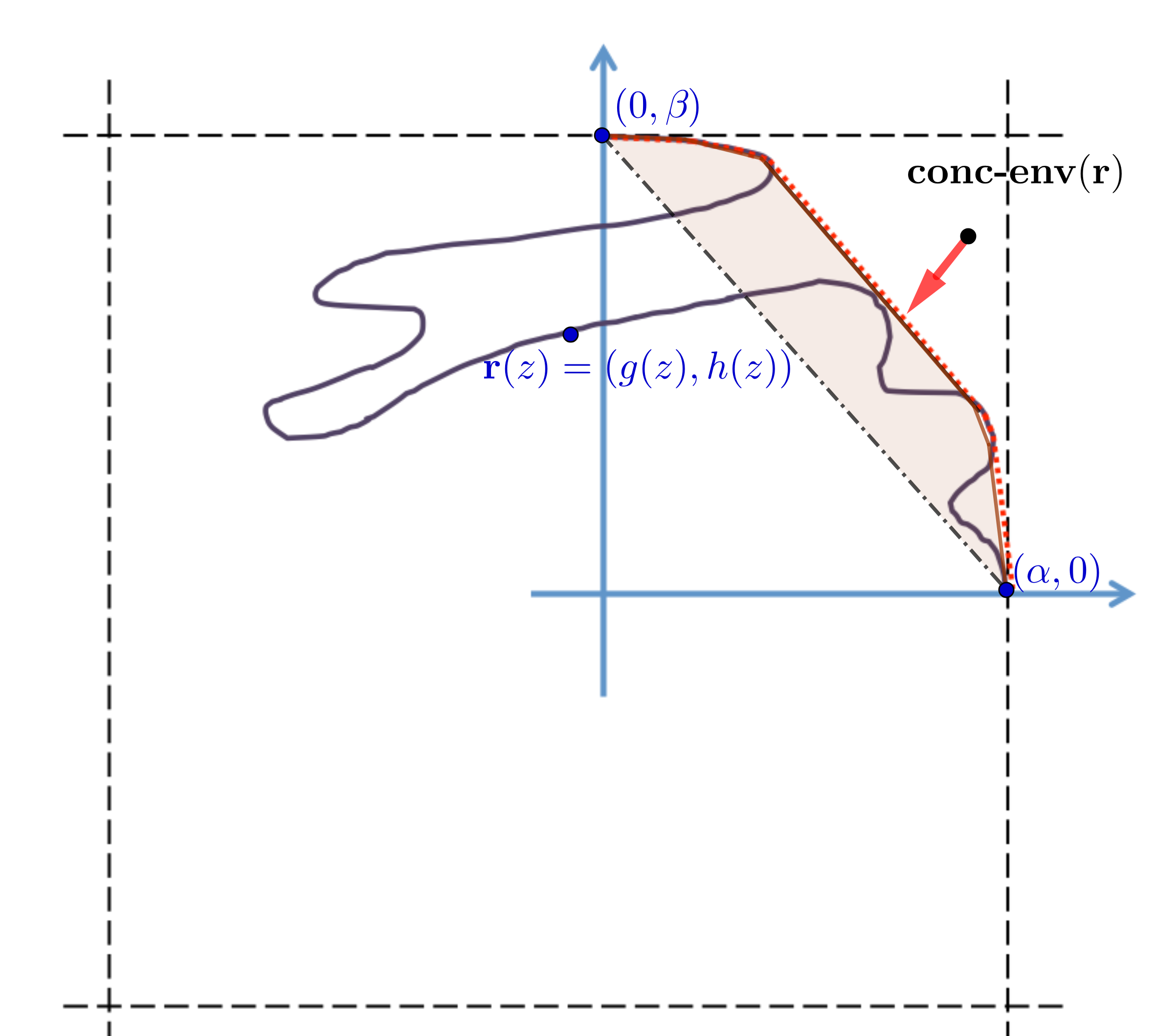
(a) Continuous curve $\mathbf{r}(z)$ in $\mathbb{R}^{2}$ (dark blue), positive-orthant concave envelope (red).

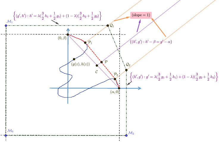
(b) Pentagon $(\mathcal{M}_{0},\mathcal{M}_{1},\mathcal{Q}_{1},\mathcal{Q}_{2},\mathcal{M}_{2})$= ADV player’s positive region against a mixed strategyover two points $\mathcal{P}_{1}$ and $\mathcal{P}_{2}$.

Figure 1:

We start by describing a vanilla version of our algorithm for maximizing $\mathcal{F}$ over the unit hypercube, termed as continuous randomized bi-greedy (Algorithm 1). This version assumes blackbox oracle access to algorithms for a few computations involving univariate functions of the form $\mathcal{F}(.,\textbf{x}_{-i})$ (e.g. maximization over $[0,1]$, computing conc-env(.), etc.). We first prove that the vanilla algorithm finds a solution with an objective value of at least $\frac{1}{2}$ of the optimum. In Section 2.2, we show how to approximately implement these oracles in polynomial time when $\mathcal{F}$ is coordinate-wise Lipschitz.

input: function $\mathcal{F}:[0,1]^{n}\rightarrow[0,1]$ ;

output: vector $\mathbf{\hat{z}}=(\hat{z}_{1},\ldots,\hat{z}_{n})\in[0,1]^{n}$ ;

Initialize $\mathbf{X}\leftarrow(0,\ldots,0)$ and $\mathbf{Y}\leftarrow(1,\ldots,1)$ ;

for $i=1$ to $n$ do

       Find ${Z}_{u},{Z}_{l}\in[0,1]$ such that $\begin{cases}{Z}_{l}\in\underset{z\in[0,1]}{\operatorname{argmax}}~{}\mathcal{F}(z,\mathbf{Y}_{-i})\\ {Z}_{u}\in\underset{z\in[0,1]}{\operatorname{argmax}}~{}\mathcal{F}(z,\mathbf{X}_{-i})\end{cases}$ ;

      

      if ${Z}_{u}\leq{Z}_{l}$ then

            $\hat{z}_{i}\leftarrow{Z}_{l}~{};$

      else

            $\forall z\in[{Z}_{l},{Z}_{u}]$, let $\begin{cases}g(z)\triangleq\mathcal{F}(z,\mathbf{X}_{-i})-\mathcal{F}({Z}_{l},\mathbf{X}_{-i}),\\ h(z)\triangleq\mathcal{F}(z,\mathbf{Y}_{-i})-\mathcal{F}({Z}_{u},\mathbf{Y}_{-i}),\end{cases}$ ;

            

            Let $\alpha\triangleq g({Z}_{u})$ and $\beta\triangleq h({Z}_{l})$ ;        // note that $\mathtt{\alpha},\mathtt{\beta}\geq 0$

            

            Let $\textbf{r}(z)\triangleq\left(g(z),h(z)\right)$ be a continuous two-dimensional curve in $[-1,\alpha]\times[-1,\beta]$ ;

            

            Compute $\texttt{conc-env}(\textbf{r})$ (i.e. positive-orthant concave envelope of $\textbf{r}(t)$ as in Definition 3) ;

            

            Find point $\mathcal{P}\triangleq~{}$intersection of $\texttt{conc-env}(\textbf{r})$ and the line $h^{\prime}-\beta=g^{\prime}-\alpha$ on g-h plane ;

            

            Suppose $\mathcal{P}=\lambda\mathcal{P}_{1}+(1-\lambda)\mathcal{P}_{2}$, where $\lambda\in[0,1]$ and $\mathcal{P}_{j}=\textbf{r}(z^{(j)}),z^{(j)}\in[{Z}_{l},{Z}_{u}]$ for $~{}~{}~{}~{}~{}~{}~{}~{}~{}~{}~{}~{}~{}j=1,2$, and both points are also on the conc-env(r) ;      // see Figure 1(b)

            

            Randomly pick $\hat{z}_{i}$ such that $\begin{cases}\hat{z}_{i}\leftarrow z^{(1)}~{}~{}~{}\textrm{with probablity}~{}\lambda\\ \hat{z}_{i}\leftarrow z^{(2)}~{}~{}~{}\textrm{o.w.}\end{cases}$ ;

      

      Let $X_{i}\leftarrow\hat{z}_{i}$ and $Y_{i}\leftarrow\hat{z}_{i}$ ;      // after this, $\mathbf{X}$ and $\mathbf{Y}$ will agree on coordinate $i$

      

return $\mathbf{\hat{z}}=(\hat{z}_{1},\ldots,\hat{z}_{n})$

Algorithm 1 (Vanilla) Continuous Randomized Bi-Greedy

Theorem 1.

If $\mathcal{F}(\cdot)$ is non-negative and continuous submodular (or equivalently is weak DR-SM), then Algorithm 1 is a randomized $\frac{1}{2}$-approximation algorithm, i.e. returns $\mathbf{\hat{z}}\in[0,1]^{n}$ s.t.

$$2\mbox{\rm\bf E}\left[\mathcal{F}(\mathbf{\hat{z}})\right]\geq\mathcal{F}(\mathbf{x^{*}}),~{}~{}~{}~{}~{}~{}~{}~{}~{}~{}\textrm{where $\mathbf{x^{*}}\in\underset{\textbf{x}\in[0,1]^{n}}{\operatorname{argmax}}~{}\mathcal{F}(\textbf{x})$ is the optimal solution.}$$

2.1 Analysis of the Continuous Randomized Bi-Greedy (proof of Theorem 1)

We start by defining these vectors, used in our analysis in the same spirit as Buchbinder et al. (2015):

$$i\in[n]:~{}\mathbf{X}^{(i)}\triangleq(\hat{z}_{1},\ldots,\hat{z}_{i},0,0,\ldots,0),~{}~{}~{}~{}~{}~{}\mathbf{X}^{(0)}\triangleq(0,\ldots,0)$$

$$i\in[n]:~{}\mathbf{Y}^{(i)}\triangleq(\hat{z}_{1},\ldots,\hat{z}_{i},1,1,\ldots,1),~{}~{}~{}~{}~{}~{}\mathbf{Y}^{(0)}\triangleq(1,\ldots,1)$$

$$i\in[n]:~{}\mathbf{O}^{(i)}\triangleq(\hat{z}_{1},\ldots,\hat{z}_{i},x^{*}_{i+1},\ldots,x^{*}_{n}),~{}~{}~{}\mathbf{O}^{(0)}\triangleq(x^{*}_{1},\ldots,x^{*}_{n})$$

Note that $\mathbf{X}^{(i)}$ and $\mathbf{Y}^{(i)}$ (or $\mathbf{X}^{(i-1)}$ and $\mathbf{Y}^{(i-1)}$) are the values of $\mathbf{X}$ and $\mathbf{Y}$ at the end of (or at the beginning of) the $i^{\textrm{th}}$ iteration of Algorithm 1. In the remainder of this section, we give the high-level proof ideas and present some proof sketches. See the supplementary materials for the formal proofs.

2.1.1 Reduction to coordinate-wise zero-sum games.

For each coordinate $i\in[n]$, we consider a sub-problem. In particular, define a two-player zero-sum game played between the algorithm player (denoted by ALG) and the adversary player (denoted by ADV). ALG selects a (randomized) strategy $\hat{z}_{i}\in[0,1]$, and ADV selects a (randomized) strategy $x^{*}_{i}\in[0,1]$. Recall the descriptions of $g(z)$ and $h(z)$ at iteration $i$ of Algorithm 1,:

$$g(z)=\mathcal{F}(z,\mathbf{X}_{-i}^{(i-1)})-\mathcal{F}({Z}_{l},\mathbf{X}_{-i}^{(i-1)})~{}~{},~{}~{}h(z)=\mathcal{F}(z,\mathbf{Y}_{-i}^{(i-1)})-\mathcal{F}({Z}_{u},\mathbf{Y}_{-i}^{(i-1)}).$$

We now define the utility of ALG (negative of the utility of ADV) in our zero-sum game as follows:

$$\mathcal{V}^{(i)}(\hat{z}_{i},x^{*}_{i})\triangleq\frac{1}{2}g(\hat{z}_{i})+\frac{1}{2}h(\hat{z}_{i})-\max\left(g(x^{*}_{i})-g(\hat{z}_{i}),h(x^{*}_{i})-h(\hat{z}_{i})\right).$$ (1)

Suppose the expected utility of ALG is non-negative at the equilibrium of this game. In particular, suppose ALG’s randomized strategy $\hat{z}_{i}$ (in Algorithm 1) guarantees that for every strategy $x^{*}_{i}$ of ADV the expected utility of ALG is non-negative. If this statement holds for all of the zero-sum games corresponding to different iterations $i\in[n]$, then Algorithm 1 is a $\frac{1}{2}$-approximation of the optimum.

Lemma 1.

If $\forall i\in[n]:\mbox{\rm\bf E}\left[\mathcal{V}^{(i)}(\hat{z}_{i},x^{*}_{i})\right]\geq-\delta/n$ for constant $\delta>0$, then $2\mbox{\rm\bf E}\left[\mathcal{F}(\mathbf{\hat{z}})\right]\geq\mathcal{F}(\mathbf{x^{*}})-\delta$.

Proof sketch..

Our bi-greedy approach, á la Buchbinder et al. (2015), revolves around analyzing the evolving values of three points: $\mathbf{X}^{(i)}$, $\mathbf{Y}^{(i)}$, and $\mathbf{O}^{(i)}$. These three points begin at all-zeroes, all-ones, and the optimum solution, respectively, and converge to the algorithm’s final point. In each iteration, we aim to relate the total increase in value of the first two points with the decrease in value of the third point. If we can show that the former quantity is at least twice the latter quantity, then a telescoping sum proves that the algorithm’s final choice of point scores at least half that of optimum.

The utility of our game is specifically engineered to compare the total increase in value of the first two points with the decrease in value of the third point. The positive term of the utility is half of this increase in value, and the negative term is a bound on how large in magnitude the decrease in value may be. As a result, an overall nonnegative utility implies that the increase beats the decrease by a factor of two, exactly the requirement for our bi-greedy approach to work. Finally, an additive slack of $\delta/n$ in the utility of each game sums over $n$ iterations for a total slack of $\delta$. ∎

Proof of Lemma 1..

Consider a realization of $\hat{z}_{i}$ where $\hat{z}_{i}\geq x^{*}_{i}$. We have:

$$\mathcal{F}(\mathbf{O}^{(i-1)})-\mathcal{F}(\mathbf{O}^{(i)}) =\mathcal{F}(\hat{z}_{1},\ldots,\hat{z}_{i-1},x^{*}_{i},x^{*}_{i+1},\ldots,x^{*}_{n})-\mathcal{F}(\hat{z}_{1},\ldots,\hat{z}_{i-1},\hat{z}_{i},x^{*}_{i+1},\ldots,x^{*}_{n})$$

$$\leq\mathcal{F}(\hat{z}_{1},\ldots,\hat{z}_{i-1},x^{*}_{i},1,\ldots,1)-\mathcal{F}(\hat{z}_{1},\ldots,\hat{z}_{i-1},\hat{z}_{i},1,\ldots,1)$$

$$=\left(\mathcal{F}(x^{*}_{i},\mathbf{Y}_{-i}^{(i-1)})-\mathcal{F}({Z}_{u},\mathbf{Y}_{-i}^{(i-1)})\right)-\left(\mathcal{F}(\hat{z}_{i},\mathbf{Y}_{-i}^{(i-1)})-\mathcal{F}({Z}_{u},\mathbf{Y}_{-i}^{(i-1)})\right)$$

$$=h(x^{*}_{i})-h(\hat{z}_{i}),$$ (2)

where the inequality holds due to weak DR-SM. Similarly, for a a realization of $\hat{z}_{i}$ where $\hat{z}_{i}\leq x^{*}_{i}$:

$$\mathcal{F}(\mathbf{O}^{(i-1)})-\mathcal{F}(\mathbf{O}^{(i)}) =\mathcal{F}(\hat{z}_{1},\ldots,\hat{z}_{i-1},x^{*}_{i},x^{*}_{i+1},\ldots,x^{*}_{n})-\mathcal{F}(\hat{z}_{1},\ldots,\hat{z}_{i-1},\hat{z}_{i},x^{*}_{i+1},\ldots,x^{*}_{n})$$

$$\leq\mathcal{F}(\hat{z}_{1},\ldots,\hat{z}_{i-1},x^{*}_{i},0,\ldots,0)-\mathcal{F}(\hat{z}_{1},\ldots,\hat{z}_{i-1},\hat{z}_{i},0,\ldots,0)$$

$$=\left(\mathcal{F}(x^{*}_{i},\mathbf{X}_{-i}^{(i-1)})-\mathcal{F}({Z}_{l},\mathbf{X}_{-i}^{(i-1)})\right)-\left(\mathcal{F}(\hat{z}_{i},\mathbf{X}_{-i}^{(i-1)})-\mathcal{F}({Z}_{l},\mathbf{X}_{-i}^{(i-1)})\right)$$

$$=g(x^{*}_{i})-g(\hat{z}_{i})$$ (3)

Putting eq. 2 and eq. 3 together, for every realization $\hat{z}_{i}$ we have:

$$F(\mathbf{O}^{(i-1)})-\mathcal{F}(\mathbf{O}^{(i)})\leq\max\left(g(x^{*}_{i})-g(\hat{z}_{i}),h(x^{*}_{i})-h(\hat{z}_{i})\right)$$ (4)

Moreover, consider the term $\mathcal{F}(\mathbf{X}^{(i)})-\mathcal{F}(\mathbf{X}^{(i-1)})$. We have:

$$\mathcal{F}(\mathbf{X}^{i})-\mathcal{F}(\mathbf{X}^{(i-1)}) =\mathcal{F}(\hat{z}_{1},\ldots,\hat{z}_{i-1},\hat{z}_{i},0,\ldots,0)-\mathcal{F}(\hat{z}_{1},\ldots,\hat{z}_{i-1},0,0,\ldots,0)$$

$$=g(\hat{z}_{i})-g(0)=g(\hat{z}_{i})+\mathcal{F}({Z}_{l},\mathbf{X}_{-i}^{(i-1)})-\mathcal{F}(\mathbf{X}^{(i-1)})$$

$$\geq g(\hat{z}_{i})+\mathcal{F}({Z}_{l},\mathbf{Y}_{-i}^{(i-1)})-\mathcal{F}(0,\mathbf{Y}_{-i}^{(i-1)})\geq g(\hat{z}_{i})$$ (5)

where the first inequality holds due to weak DR-SM property and the second inequity holds as ${Z}_{l}\in\underset{z\in[0,1]}{\operatorname{argmax}}~{}\mathcal{F}(z,\mathbf{Y}_{-i}^{(i-1)})$. Similarly, consider the term $\mathcal{F}(\mathbf{Y}^{(i)})-\mathcal{F}(\mathbf{Y}^{(i-1)})$. We have:

$$\mathcal{F}(\mathbf{Y}^{(i)})-\mathcal{F}(\mathbf{Y}^{(i-1)}) =\mathcal{F}(\hat{z}_{1},\ldots,\hat{z}_{i-1},\hat{z}_{i},1,\ldots,1)-\mathcal{F}(\hat{z}_{1},\ldots,\hat{z}_{i-1},1,1,\ldots,1)$$

$$=h(\hat{z}_{i})-h(1)=h(\hat{z}_{i})+\mathcal{F}({Z}_{u},\mathbf{Y}_{-i}^{(i-1)})-\mathcal{F}(\mathbf{Y}^{(i-1)})$$

$$\geq h(\hat{z}_{i})+\mathcal{F}({Z}_{u},\mathbf{X}_{-i}^{(i-1)})-\mathcal{F}(1,\mathbf{X}_{-i}^{(i-1)})\geq h(\hat{z}_{i})$$ (6)

where the first inequality holds due to weak DR-SM and the second inequity holds as ${Z}_{u}\in\underset{z\in[0,1]}{\operatorname{argmax}}~{}\mathcal{F}(z,\mathbf{X}_{-i}^{(i-1)})$. By eq. 4, eq. 5, eq. 6, and the fact that $\mathcal{F}(\mathbf{0})+\mathcal{F}(\mathbf{1})\geq 0$, we have:

$$0 \leq\displaystyle\sum_{i=1}^{n}{\mbox{\rm\bf E}\left[\mathcal{V}^{(i)}(\hat{z}_{i},x^{*}_{i})\right]}=\displaystyle\sum_{i=1}^{n}\left({\frac{1}{2}\mbox{\rm\bf E}\left[g(\hat{z}_{i})\right]+\frac{1}{2}\mbox{\rm\bf E}\left[h(\hat{z}_{i})\right]-\mbox{\rm\bf E}\left[\max\left(g(x^{*}_{i})-g(\hat{z}_{i}),h(x^{*}_{i})-h(\hat{z}_{i})\right)\right]}\right)$$

$$\leq\frac{1}{2}\displaystyle\sum_{i=1}^{n}\left(\mathcal{F}(\mathbf{X}^{(i)})-\mathcal{F}(\mathbf{X}^{(i-1)})\right)+\frac{1}{2}\displaystyle\sum_{i=1}^{n}\left(\mathcal{F}(\mathbf{Y}^{(i)})-\mathcal{F}(\mathbf{Y}^{(i-1)})\right)-\displaystyle\sum_{i=1}^{n}\left(\mathcal{F}(\mathbf{O}^{(i-1)})-\mathcal{F}(\mathbf{O}^{(i)})\right)$$

$$=\frac{\mathcal{F}(\mathbf{X}^{(n)})-\mathcal{F}(\mathbf{X}^{(0)})}{2}+\frac{\mathcal{F}(\mathbf{Y}^{(n)})-\mathcal{F}(\mathbf{Y}^{(0)})}{2}-\mathcal{F}(\mathbf{O}^{(0)})+\mathcal{F}(\mathbf{O}^{(n)})$$

$$\leq\frac{\mathcal{F}(\mathbf{\hat{z}})}{2}+\frac{\mathcal{F}(\mathbf{\hat{z}})}{2}-\mathcal{F}(\mathbf{x^{*}})+\mathcal{F}(\mathbf{\hat{z}})=2\mathcal{F}(\mathbf{\hat{z}})-\mathcal{F}(\mathbf{x^{*}})\qed$$

2.1.2 Analyzing the zero-sum games.

Fix an iteration $i\in[n]$ of Algorithm 1. We then have the following.

Proposition 1.

If ALG plays the (randomized) strategy $\hat{z}_{i}$ as described in Algorithm 1, then we have $\mbox{\rm\bf E}\left[\mathcal{V}^{(i)}(\hat{z}_{i},x^{*}_{i})\right]\geq 0$ against any strategy $x^{*}_{i}$ of ADV.

Proof of Proposition 1.

We do the proof by case analysis over two cases:

$\square~{}$ Case $\mathbf{{Z}_{l}\geq{Z}_{u}}$ (easy):

In this case, the algorithm plays a deterministic strategy $\hat{z}_{i}={Z}_{l}$. We therefore have:

$$\mathcal{V}^{(i)}(\hat{z}_{i},x^{*}_{i})=\frac{1}{2}g(\hat{z}_{i})+\frac{1}{2}h(\hat{z}_{i})-\max\left(g(x^{*}_{i})-g(\hat{z}_{i}),h(x^{*}_{i})-h(\hat{z}_{i})\right)\geq\min(g(\hat{z}_{i})-g(x^{*}_{i}),0)$$

where the inequality holds because $g(\hat{z}_{i})=g({Z}_{l})=0$, and also ${Z}_{l}\in\underset{z\in[0,1]}{\operatorname{argmax}}~{}\mathcal{F}(z,\mathbf{Y}_{-i}^{(i)})$ and so:

• $h(\hat{z}_{i})=h({Z}_{l})=\mathcal{F}({Z}_{l},\mathbf{Y}_{-i}^{(i)})-\mathcal{F}({Z}_{u},\mathbf{Y}_{-i}^{(i)})\geq 0$

• $h(x^{*}_{i})-h(\hat{z}_{i})=\mathcal{F}(x^{*}_{i},\mathbf{Y}_{-i}^{(i-1)})-\mathcal{F}({Z}_{l},\mathbf{Y}_{-i}^{(i-1)})\leq 0$

To complete the proof for this case, it is only remained to show $g(\hat{z}_{i})-g(x^{*}_{i})\geq 0$. As ${Z}_{l}\geq{Z}_{u}$, for any given $x^{*}_{i}\in[0,1]$ either $x^{*}_{i}\leq{Z}_{l}$ or $x^{*}_{i}\geq{Z}_{u}$ (or both). If $x^{*}_{i}\leq{Z}_{l}$ then:

$$g(\hat{z}_{i})-g(x^{*}_{i})=-g(x^{*}_{i})=\mathcal{F}({Z}_{l},\mathbf{X}^{(i-1)}_{-i})-\mathcal{F}(x^{*}_{i},\mathbf{X}^{(i-1)}_{-i})\geq\mathcal{F}({Z}_{l},\mathbf{Y}^{(i-1)}_{-i})-\mathcal{F}(x^{*}_{i},\mathbf{Y}^{(i-1)}_{-i})\geq 0$$

where the first inequality uses weak DR-SM property and the second inequality uses the fact ${Z}_{l}\in\underset{z\in[0,1]}{\operatorname{argmax}}~{}\mathcal{F}(z,\mathbf{Y}_{-i}^{(i)})$. If $x^{*}_{i}\leq{Z}_{u}$, we then have:

$$g(\hat{z}_{i})-g(x^{*}_{i}) =\mathcal{F}({Z}_{l},\mathbf{X}^{(i-1)}_{-i})-\mathcal{F}(x^{*}_{i},\mathbf{X}^{(i-1)}_{-i})$$

$$=\mathcal{F}({Z}_{l},\mathbf{X}^{(i-1)}_{-i})-\mathcal{F}({Z}_{u},\mathbf{X}^{(i-1)}_{-i})+\mathcal{F}({Z}_{u},\mathbf{X}^{(i-1)}_{-i})-\mathcal{F}(x^{*}_{i},\mathbf{X}^{(i-1)}_{-i})$$

$$\geq\left(\mathcal{F}({Z}_{l},\mathbf{Y}^{(i-1)}_{-i})-\mathcal{F}({Z}_{u},\mathbf{Y}^{(i-1)}_{-i})\right)+\left(\mathcal{F}({Z}_{u},\mathbf{X}^{(i-1)}_{-i})-\mathcal{F}(x^{*}_{i},\mathbf{X}^{(i-1)}_{-i})\right)\geq 0$$

where the first inequality uses weak DR-SM property and the second inequality holds because both terms are non-negative, following the fact that:

$${Z}_{l}\in\underset{z\in[0,1]}{\operatorname{argmax}}~{}\mathcal{F}(z,\mathbf{Y}_{-i}^{(i)})~{}~{}~{}~{}~{}~{}~{}~{}\textrm{and}~{}~{}~{}~{}~{}~{}~{}~{}{Z}_{u}\in\underset{z\in[0,1]}{\operatorname{argmax}}~{}\mathcal{F}(z,\mathbf{X}_{-i}^{(i)})$$

Therefore, we finish the proof of the easy case.

$\square~{}$ Case $\mathbf{{Z}_{l}<{Z}_{u}}$ (hard):

In this case, ALG plays a mixed strategy over two points. To determine the two-point support, it considers the curve $\textbf{r}=\{(g(z),h(z))\}_{z\in[{Z}_{l},{Z}_{u}]}$ and finds a point $\mathcal{P}$ on $\texttt{conc-env}(\textbf{r})$ (i.e., Definition 3) that lies on the line $h^{\prime}-\beta=g^{\prime}-\alpha$, where recall that $\alpha=g({Z}_{u})\geq 0$ and $\beta=g({Z}_{l})\geq 0$ (as ${Z}_{u}$ and ${Z}_{l}$ are the maximizers of $\mathcal{F}(z,\mathbf{X}_{-i}^{(i-1)})$ and $\mathcal{F}(z,\mathbf{Y}_{-i}^{(i-1)})$ respectively). Because this point is on the concave envelope it should be a convex combination of two points on the curve $\textbf{r}(z)$. Lets say $\mathcal{P}=\lambda\mathcal{P}_{1}+(1-\lambda)\mathcal{P}_{2}$, where $\mathcal{P}_{1}=\textbf{r}(z^{(1)})$ and $\mathcal{P}_{2}=\textbf{r}(z^{(2)})$, and $\lambda\in[0,1]$. The final strategy of ALG is a mixed strategy over $\{z^{(1)},z^{(2)}\}$ with probabilities $(\lambda,1-\lambda)$. Fixing any mixed strategy of ALG over two points $\mathcal{P}_{1}=(g_{1},h_{1})$ and $\mathcal{P}_{2}=(g_{2},h_{2})$ with probabilities $(\lambda,1-\lambda)$ (denoted by $\mathcal{F_{\mathcal{P}}}$), define the ADV’s positive region, i.e.

$$(g^{\prime},h^{\prime})\in[-1,1]\times[-1,1]:~{}~{}\mathbf{E}_{(g,h)\sim F_{\mathcal{P}}}\left[{\frac{1}{2}g+\frac{1}{2}h-\max(g^{\prime}-g,h^{\prime}-h)}\right]\geq 0.$$

Now, suppose ALG plays a mixed strategy with the property that its corresponding ADV’s positive region covers the entire curve $\{g(z),h(z)\}_{z\in[0,1]}$. Then, for any strategy $x^{*}_{i}$ of ADV the expected utility of ALG is non-negative. In the rest of the proof, we geometrically characterize the ADV’s positive region against a mixed strategy of ALG over a 2-point support, and then we show for the particular choice of $\mathcal{P}_{1}$, $\mathcal{P}_{2}$ and $\lambda$ in Algorithm 1 the positive region covers the entire curve $\{g(z),h(z)\}_{z\in[0,1]}$.

Lemma 2.

Suppose ALG plays a 2-point mixed strategy over $\mathcal{P}_{1}=\textbf{r}(z^{(1)})=(g_{1},h_{1})$ and $\mathcal{P}_{2}=\textbf{r}(z^{(1)})=(g_{2},h_{2})$ with probabilities $(\lambda,1-\lambda)$, and w.l.o.g. $h_{1}-g_{1}\geq h_{2}-g_{2}$. Then ADV’s positive region is the pentagon $(\mathcal{M}_{0},\mathcal{M}_{1},\mathcal{Q}_{1},\mathcal{Q}_{2},\mathcal{M}_{2})$, where $\mathcal{M}_{0}=(-1,-1)$ and (see Figure 1(b)):

1. $\mathcal{M}_{1}=\left(-1,\lambda(\frac{3}{2}h_{1}+\frac{1}{2}g_{1})+(1-\lambda)(\frac{3}{2}h_{2}+\frac{1}{2}g_{2})\right)$,

2. $\mathcal{M}_{2}=\left(\lambda(\frac{3}{2}g_{1}+\frac{1}{2}h_{1})+(1-\lambda)(\frac{3}{2}g_{2}+\frac{1}{2}h_{2}),-1\right)$,

3. $\mathcal{Q}_{1}$ is the intersection of the lines leaving $\mathcal{P}_{1}$ with slope $1$ and leaving $\mathcal{M}_{1}$ along the g-axis,

4. $\mathcal{Q}_{2}$ is the intersection of the lines leaving $\mathcal{P}_{2}$ with slope $1$ and leaving $\mathcal{M}_{2}$ along the h-axis.

Proof of Lemma 2..

We start by a technical lemma, showing a single-crossing property of the g-h curve of a weak DR submodular function $\mathcal{F}(.)$, and we then characterize the region using this lemma.

Lemma 3.

The univariate function $d(z)=h(z)-g(z)$ is monotone non-increasing.

Proof.

By using weak DR-SM property of $\mathcal{F}(.)$ the proof is immediate, as for any $\delta\geq 0$,

$$d(z+\delta)-d(z)=\left(\mathcal{F}(z+\delta,\mathbf{Y}^{(i-1)}_{-i})-\mathcal{F}(z,\mathbf{Y}^{(i-1)}_{-i})\right)-(F(z+\delta,\mathbf{X}^{(i-1)}_{-i})-F(z+\delta,\mathbf{X}^{(i-1)}_{-i}))\leq 0,$$

where the inequality holds due to the fact that $\mathbf{Y}^{(i-1)}_{-i}\geq\mathbf{X}^{(i-1)}_{-i}$ and $\delta\geq 0$. ∎

Being equipped with Lemma 3, the positive region is the set of all points $(g^{\prime},h^{\prime})\in[-1,1]^{2}$ such that

$$\mathbf{E}_{(g,h)\sim F_{\mathcal{P}}}\left[{\frac{1}{2}g+\frac{1}{2}h-\max(g^{\prime}-g,h^{\prime}-h)}\right]$$

$$=\lambda\left(\frac{1}{2}g_{1}+\frac{1}{2}h_{1}-\max(g^{\prime}-g_{1},h^{\prime}-h_{1})\right)+(1-\lambda)\left(\frac{1}{2}g_{2}+\frac{1}{2}h_{2}-\max(g^{\prime}-g_{2},h^{\prime}-h_{2})\right)\geq 0$$

The above inequality defines a polytope. Our goal is to find the vertices and faces of this polytope. Now, to this end, we only need to consider three cases: 1) $h^{\prime}-g^{\prime}\geq h_{1}-g_{1}$, 2) $h_{2}-g_{2}\leq h^{\prime}-g^{\prime}\leq h_{1}-g_{1}$ and 3) $h^{\prime}-g^{\prime}\leq h_{2}-g_{2}$ (note that $h_{1}-g_{1}\geq h_{2}-g_{2}$). From the first and third case we get the half-spaces $h^{\prime}\leq\lambda(\frac{3}{2}h_{1}+\frac{1}{2}g_{1})+(1-\lambda)(\frac{3}{2}h_{2}+\frac{1}{2}g_{2})$ and $g^{\prime}\leq\lambda(\frac{3}{2}g_{1}+\frac{1}{2}h_{1})+(1-\lambda)(\frac{3}{2}g_{2}+\frac{1}{2}h_{2})$ respectively, that form two of the faces of the positive-region polytope. From the second case, we get another half-space, but the observation is that the transition from first case to second case happens when $h^{\prime}-g^{\prime}=h_{1}-g_{1}$, i.e. on a line with slope one leaving $\mathcal{P}_{1}$, and transition from second case to the third case happens when $h^{\prime}-g^{\prime}=h_{2}-g_{2}$, i.e. on a line with slope one leaving $\mathcal{P}_{2}$. Therefore, the second half-space is the region under the line connecting two points $\mathcal{Q}_{1}$ and $\mathcal{Q}_{2}$, where $\mathcal{Q}_{1}$ is the intersection of $h^{\prime}=\lambda(\frac{3}{2}h_{1}+\frac{1}{2}g_{1})+(1-\lambda)(\frac{3}{2}h_{2}+\frac{1}{2}g_{2})$ and the line leaving $\mathcal{P}_{1}$ with slope one (point $\mathcal{Q}_{1}$), and $\mathcal{Q}_{2}$ is the intersection of $g^{\prime}=\lambda(\frac{3}{2}g_{1}+\frac{1}{2}h_{1})+(1-\lambda)(\frac{3}{2}g_{2}+\frac{1}{2}h_{2})$ and the line leaving $\mathcal{P}_{2}$ with slope one (point $\mathcal{Q}_{2}$). The line segment $\mathcal{Q}_{1}-\mathcal{Q}_{2}$ defines another face of the positive region polytope, and $\mathcal{Q}_{1}$ and $\mathcal{Q}_{2}$ will be two vertices on this face. By intersecting the three mentioned half-spaces with $g^{\prime}\geq-1$ and $h\geq-1$ (which define the two remaining faces of the positive region polytope), the postive region will be the polytope defined by the pentagon $(\mathcal{M}_{0},\mathcal{M}_{1},\mathcal{Q}_{1},\mathcal{Q}_{2},\mathcal{M}_{2})$, as claimed (see Figure 1(b) for a pictorial proof). ∎

By applying Lemma 2, we have the following main technical lemma. The proof is geometric and is pictorially visible in Figure 1(b). This lemma finishes the proof of Proposition 1.

Lemma 4 (main lemma).

If ALG plays the two point mixed strategy described in Algorithm 1, then for every $x^{*}_{i}\in[0,1]$ the point $(g^{\prime},h^{\prime})=\left(g(x^{*}_{i}),h(x^{*}_{i})\right)$ is in the ADV’s positive region.

Proof sketch..

For simplicity assume ${Z}_{l}=0$ and ${Z}_{u}=1$. To understand the ADV’s positive region that results from playing a two-point mixed strategy by ALG, we consider the positive region that results from playing a one point pure strategy. When ALG chooses a point $(g,h)$, the positive term of the utility is one-half of its one-norm. The negative term of the utility is the worse between how much the ADV’s point is above ALG’s point, and how much it is to the right of ALG’s point. The resulting positive region is defined by an upper boundary $g^{\prime}\leq\frac{3}{2}g+\frac{1}{2}h$ and a right boundary $h^{\prime}\leq\frac{1}{2}g+\frac{3}{2}h$.

Next, let’s consider what happens when we pick point $(g_{1},h_{1})$ with probability $\lambda$ and point $(g_{2},h_{2})$ with probability $(1-\lambda)$. We can compute the expected point: let $(g_{3},h_{3})=\lambda(g_{1},h_{1})+(1-\lambda)(g_{2},h_{2})$. As suggested by Lemma 2, the positive region for our mixed strategy has three boundary conditions: an upper boundary, a right boundary, and a corner-cutting boundary. The first two boundary conditions correspond to a pure strategy which picks $(g_{3},h_{3})$. By design, $(g_{3},h_{3})$ is located so that these boundaries cover the entire $[-1,\alpha]\times[-1,\beta]$ rectangle. This leaves us with analyzing the corner-cutting boundary, which is the focus of Figure 1(b). As it turns out, the intersections of this boundary with the two other boundaries lie on lines of slope $1$ extending from $(g_{j},h_{j})_{j=1,2}$. If we consider the region between these two lines, the portion under the envelope (where the curve r may lie) is distinct from the portion outside the corner-cutting boundary. However, if r were to ever violate the corner-cutting boundary condition without violating the other two boundary conditions, it must do so in this region. Hence the resulting positive region covers the entire curve r, as desired. ∎

Proof of Lemma 4.

First of a all, we claim any ADV’s strategy $x^{*}_{i}\in[0,{Z}_{l})$ (or $x^{*}_{i}\in({Z}_{u},1]$) is weakly dominated by ${Z}_{l}$ (or ${Z}_{u}$) if ALG plays a (randomized) strategy $\hat{z}_{i}\in[{Z}_{l},{Z}_{u}]$. To see this, if $x^{*}_{i}\in[0,{Z}_{l})$,

$$\max\left(g(x^{*}_{i})-g(\hat{z}_{i}),h(x^{*}_{i})-h(\hat{z}_{i})\right)$$

$$=\max\left(\mathcal{F}(x^{*}_{i},\mathbf{X}^{(i-1)}_{-i})-\mathcal{F}(\hat{z}_{i},\mathbf{X}^{(i-1)}_{-i}),\mathcal{F}(x^{*}_{i},\mathbf{Y}^{(i-1)}_{-i})-\mathcal{F}(\hat{z}_{i},\mathbf{Y}^{(i-1)}_{-i})\right)$$

$$=\mathcal{F}(x^{*}_{i},\mathbf{Y}^{(i-1)}_{-i})-\mathcal{F}(\hat{z}_{i},\mathbf{Y}^{(i-1)}_{-i})\leq\mathcal{F}({Z}_{l},\mathbf{Y}^{(i-1)}_{-i})-\mathcal{F}(\hat{z}_{i},\mathbf{Y}^{(i-1)}_{-i})$$

$$=h({Z}_{l})-h(\hat{z}_{i})\leq\max\left(g({Z}_{l})-g(\hat{z}_{i}),h({Z}_{l})-h(\hat{z}_{i})\right)$$

and therefore $\mathcal{V}^{(i)}(\hat{z}_{i},{Z}_{l})\leq\mathcal{V}^{(i)}(\hat{z}_{i},x^{*}_{i})$ for any $x^{*}_{i}\in[0,{Z}_{l})$. Similarly, $\mathcal{V}^{(i)}(\hat{z}_{i},{Z}_{u})\leq\mathcal{V}^{(i)}(\hat{z}_{i},x^{*}_{i})$ for any $x^{*}_{i}\in({Z}_{u},1]$. So, without loss of generality, we can assume ADV’s strategy $x^{*}_{i}$ is in $[{Z}_{l},{Z}_{u}]$.

Now, consider the curve $\textbf{r}=\{(g(z),h(z)\}_{z\in[{Z}_{l},{Z}_{u}]}$ as in Figure 1(b). ALG’s strategy is a 2-point mixed strategy over $\mathcal{P}_{1}=(g_{1},h_{1})=\textbf{r}(z^{(1)})$ and $\mathcal{P}_{2}=(g_{2},h_{2})=\textbf{r}(z^{(1)})$, where these two points are on different sides of the line $\mathcal{L}:h^{\prime}-\beta=g^{\prime}-\alpha$ (or both of them are on the line $\mathcal{L}$). Without loss of generality, assume $h_{1}-g_{1}\geq\beta-\alpha\geq h_{2}-g_{2}$. Note that $\textbf{r}({Z}_{l})=(0,\beta)$ is above the line $\mathcal{L}$ and $\textbf{r}({Z}_{l})=(\alpha,0)$ is below the line $\mathcal{L}$. So, because $h(z)-g(z)$ is monotone non-increasing due to Lemma 3, we should have ${Z}_{l}\leq z^{(1)}\leq z^{(2)}\leq{Z}_{u}$.

Using Lemma 2, the ADV’s positive region is $(\mathcal{M}_{0},\mathcal{M}_{1},\mathcal{Q}_{1},\mathcal{Q}_{2},\mathcal{M}_{2})$, where $\{\mathcal{M}_{j}\}_{j=1,2,3}$ and $\{\mathcal{Q}_{j}\}_{j=1,2}$ are as described in Lemma 2. The upper concave envelope $\texttt{conc-env}(\textbf{r})$ upper-bounds the curve r. Therefore, to show that curve r is entirely covered by the ADV’s positive region, it is only enough to show its upper concave envelope $\texttt{conc-env}(\textbf{r})$ is entirely covered (as can also be seen from Figure 1(b)). Lets denote the line leaving $\mathcal{P}_{j}$ with slope one by $\mathcal{L}_{j}$ for $j=1,2$. The curve $\texttt{conc-env}(\textbf{r})$ consists of three parts: the part above $\mathcal{L}_{1}$, the part below $\mathcal{L}_{2}$ and the part between $\mathcal{L}_{1}$ and $\mathcal{L}_{2}$ (the last part is indeed the line segment connecting $\mathcal{P}_{1}$ and $\mathcal{P}_{2}$). Interestingly, the line connecting $\mathcal{P}_{1}$ to $\mathcal{Q}_{1}$ and the line connecting $\mathcal{P}_{2}$ to $\mathcal{Q}_{2}$ both have slope $1$. So, as it can be seen from Figure 1(b), if we show $\mathcal{Q}_{1}$ is above the line $h^{\prime}=\beta$ and $\mathcal{Q}_{2}$ is to the right of the line $g^{\prime}=\alpha$, then the $\texttt{conc-env}(\textbf{r})$ will entirely be covered by the positive region and we are done. To see why this holds, first note that $\lambda$ has been picked so that $\mathcal{P}\triangleq(\mathcal{P}_{g},\mathcal{P}_{h})=\lambda\mathcal{P}_{1}+(1-\lambda)\mathcal{P}_{2})$. Due to Lemma 2,

$$\mathcal{Q}_{1},h =\lambda(\frac{3}{2}h_{1}+\frac{1}{2}g_{1})+(1-\lambda)(\frac{3}{2}h_{2}+\frac{1}{2}g_{2})=\frac{3}{2}\mathcal{P}_{h}+\frac{1}{2}\mathcal{P}_{g}$$

$$\mathcal{Q}_{2},g =\lambda(\frac{3}{2}g_{1}+\frac{1}{2}h_{1})+(1-\lambda)(\frac{3}{2}g_{2}+\frac{1}{2}h_{2})=\frac{3}{2}\mathcal{P}_{g}+\frac{1}{2}\mathcal{P}_{h}$$

Moreover, point $\mathcal{P}=(\mathcal{P}_{g},\mathcal{P}_{h})$ dominates the point $\mathcal{C}\triangleq(\frac{\alpha^{2}}{\alpha+\beta},\frac{\beta^{2}}{\alpha+\beta})$ coordinate-wise. This dominance is simply true because points $\mathcal{C}$ and $\mathcal{P}$ are actually the intersections of the line $\mathcal{L}:h^{\prime}-\beta=g^{\prime}-\alpha$ (with slope one) with the line connecting $(0,\beta)$ to $(\alpha,0)$ and with the curve $\texttt{conc-env}(\textbf{r})$ respectively. As $\texttt{conc-env}(\textbf{r})$ upper-bounds the line connecting $(0,\beta)$ to $(\alpha,0)$, and because $\mathcal{L}$ has slope one, $\mathcal{P}_{h}\geq\mathcal{C}_{h}=\frac{\beta^{2}}{\alpha+\beta}$ and $\mathcal{P}_{g}\geq\mathcal{C}_{g}=\frac{\alpha^{2}}{\alpha+\beta}$. Putting all the pieces together,

$$\mathcal{Q}_{1,h} \geq\frac{3}{2}\frac{\beta^{2}}{\alpha+\beta}+\frac{1}{2}\frac{\alpha^{2}}{\alpha+\beta}=\frac{\left(\alpha^{2}+\beta^{2}-2\alpha\beta\right)+2\beta^{2}+2\alpha\beta}{2(\alpha+\beta)}=\beta+\frac{(\alpha-\beta)^{2}}{2(\alpha+\beta)}\geq\beta$$

$$\mathcal{Q}_{2,g} \geq\frac{3}{2}\frac{\alpha^{2}}{\alpha+\beta}+\frac{1}{2}\frac{\beta^{2}}{\alpha+\beta}=\frac{\left(\alpha^{2}+\beta^{2}-2\alpha\beta\right)+2\alpha^{2}+2\alpha\beta}{2(\alpha+\beta)}=\alpha+\frac{(\alpha-\beta)^{2}}{2(\alpha+\beta)}\geq\alpha$$

which implies $\mathcal{Q}_{1}$ is above the line $h^{\prime}=\beta$ and $\mathcal{Q}_{2}$ is to the right of the line $g^{\prime}=\alpha$, as desired. ∎

∎

2.2 Polynomial-time Implementation under Lipschitz Continuity: Overview

At each iteration, Algorithm 1 interfaces with $\mathcal{F}$ in two ways: (i) when performing optimization to compute ${Z}_{l},{Z}_{u}$ and (ii) when computing the upper-concave envelope. In both cases, we are concerned with univariate projections of $\mathcal{F}$, namely $\mathcal{F}(z,\mathbf{X}_{-i})$ and $\mathcal{F}(z,\mathbf{Y}_{-i}$. Assuming $\mathcal{F}$ is coordinate-wise Lipschitz continuous with constant $C>0$, we choose a small $\epsilon>0$ and take periodic samples at $\epsilon$-spaced intervals from each one of these functions, for a total of $O(\frac{1}{\epsilon})$ samples.

To perform task (i), we simply return the the sample which resulted in the maximum function value. Since the actual maximum is $\epsilon$-close to one of the samples, our maximum is at most an additive $\epsilon C$ lower in value. To perform task (ii), we use these samples to form an approximate $\textbf{r}(z)$ curve, denoted by $\hat{\textbf{r}}(z)$. Note that we then proceed exactly as described in Algorithm 1 to pick a (randomized) strategy $\hat{z}_{i}$ using $\hat{\textbf{r}}(z)$. Note that ADV can actually choose a point on the exact curve $\textbf{r}(z)$. However the point she chooses is close to one of our samples and hence is at most an additive $\epsilon C$ better in value with respect to functions $g(.)$ and $h(.)$. Furthermore, we can compute the upper-concave envelope $\hat{\textbf{r}}(z)$ in time linear in the number of samples using Graham’s algorithm (Graham, 1972). Roughly speaking, this is because we can go through the samples in order of $z$-coordinate, avoiding the sorting cost of running Graham’s on completely unstructured data. Formally, we have the following proposition. For detailed implementations, see Algorithm 2 and Algorithm 3.

Proposition 2.

If $\mathcal{F}$ is coordinate-wise Lipschitz continuous with constant $C>0$, then there exists an implementation of Algorithm 1 that runs in time $O(n^{2}/\epsilon)$ and returns a (randomized) point $\mathbf{\hat{z}}$ s.t.

$$2\mbox{\rm\bf E}\left[\mathcal{F}(\mathbf{\hat{z}})\right]\geq\mathcal{F}(\mathbf{x^{*}})-2C\epsilon,~{}~{}~{}~{}~{}~{}~{}~{}~{}~{}\textrm{where $\mathbf{x^{*}}\in\underset{\textbf{x}\in[0,1]^{n}}{\operatorname{argmax}}~{}\mathcal{F}(\textbf{x})$ is the optimal solution.}$$

input: function $f:[0,1]\rightarrow[0,1]$, additive error $\delta>0$, Lipschitz Constant $C>0$ ;

output: coordinate value $z\in[0,1]^{n}$ ;

Set $\epsilon\leftarrow\frac{\delta}{C}$ ;

Initialize $z^{*}\leftarrow 0$ ;

Initialize $z\leftarrow 0$ ;

while $z\leq 1$ do

       if $f(z)>f(z^{*})$ then

             $z^{*}\leftarrow z$ ;

            

      $z\leftarrow z+\epsilon$ ;

      

return $z^{*}$

Algorithm 2 Approximate One-Dimensional Optimization

input: function $f:[0,1]\rightarrow[0,1]$, function $g:[0,1]\rightarrow[0,1]$, additive error $\delta>0$, Lipschitz Constant $C>0$ ;

output: stacks $s$ and $t$ ;

Set $\epsilon\leftarrow\frac{\delta}{C}$ ;

Initialize stacks $s,t$ ;

Initialize $z\leftarrow 0$ ;

while $z\leq 1$ do

       if $s$ is empty or $f(z)$ is strictly larger than the first coordinate of the the top element of $s$ then

             while $s$ has at least two elements and the slope from (the second-to-top element of $s$) to (the top element of $s$) is less than the slope from (the top element of $s$) to $(f(z),g(z))$ do

                   Pop the top element of $s$ ;

                   Pop the top element of $t$ ;

                  

            Push $(f(z),g(z))$ onto $s$ ;

             Push $z$ onto $t$ ;

            

      $z\leftarrow z+\epsilon$ ;

      

return $(s,t)$

Algorithm 3 Approximate Annotated Upper-Concave Envelope

3 Strong DR-SM Maximization: Binary-Search Bi-Greedy

Our second result is a fast binary search algorithm, achieving the tight $\frac{1}{2}$-approximation factor (up to additive error $\delta$) in quasi-linear time in $n$, but only for the special case of strong DR-SM functions (a.k.a. DR-submodular); see Definition 1. This algorithm leverages the coordinate-wise concavity to identify a coordinate-wise monotone equilibrium condition. In each iteration, it hunts for an equilibrium point by using binary search. Satisfying the equilibrium at each iteration then guarantees the desired approximation factor. Formally we propose Algorithm 4.

input: function $\mathcal{F}:[0,1]^{n}\rightarrow[0,1]$, error $\epsilon>0$ ;

output: vector $\mathbf{\hat{z}}=(\hat{z}_{1},\ldots,\hat{z}_{n})\in[0,1]^{n}$ ;

Initialize $\mathbf{X}\leftarrow(0,\ldots,0)$ and $\mathbf{Y}\leftarrow(1,\ldots,1)$ ;

for $i=1$ to $n$ do

       if $\frac{\partial\mathcal{F}}{\partial x_{i}}(0,\mathbf{X}_{-i})<0~{}~{}\&~{}~{}\frac{\partial\mathcal{F}}{\partial x_{i}}(1,\mathbf{Y}_{-i})\leq 0$ then

            $\hat{z}_{i}\leftarrow 0$

      else if $\frac{\partial\mathcal{F}}{\partial x_{i}}(0,\mathbf{X}_{-i})\geq 0~{}~{}\&~{}~{}\frac{\partial\mathcal{F}}{\partial x_{i}}(1,\mathbf{Y}_{-i})>0$ then

            $\hat{z}_{i}\leftarrow 1$

      else

             // we do binary search.

             while $Y_{i}-X_{i}>{\epsilon}/{n}$ do

                   Let $\hat{z}_{i}\leftarrow\frac{X_{i}+Y_{i}}{2}$ ;

                  

                  if $\frac{\partial\mathcal{F}}{\partial x_{i}}(\hat{z}_{i},\mathbf{X}_{-i})\cdot(1-\hat{z}_{i})+\frac{\partial\mathcal{F}}{\partial x_{i}}(\hat{z}_{i},\mathbf{Y}_{-i})\cdot\hat{z}_{i}<0$ then

                         // we need to increase $w_{i}$.

                         Set $X_{i}\leftarrow\hat{z}_{i}$ ;

                        

                  else

                         // we need to decrease $w_{i}$.

                         Set $Y_{i}\leftarrow\hat{z}_{i}$ ;

                        

                  

            

      Let $X_{i}\leftarrow\hat{z}_{i}$ and $Y_{i}\leftarrow\hat{z}_{i}$ ;       // after this, $\mathbf{X}$ and $\mathbf{Y}$ will agree at coordinate $i$

      

return $\mathbf{\hat{z}}=(\hat{z}_{1},\ldots,\hat{z}_{n})$

Algorithm 4 Binary-Search Continuous Bi-greedy

As a technical assumption, let $\mathcal{F}$ be Lipschitz continuous with some constant $C>0$, so that we can relate the precision of our binary search with additive error. We arrive at the theorem, proved in Section 3.1.

Theorem 2.

If $\mathcal{F}(.)$ is non-negative and DR-submodular (a.k.a Strong DR-SM) and is coordinate-wise Lipschitz continuous with constant $C>0$, then Algorithm 4 runs in time $O\left(n\log(\frac{n}{\epsilon})\right)$ and is a deterministic $\frac{1}{2}$-approximation algorithm up to $O(\epsilon)$ additive error, i.e. returns $\mathbf{\hat{z}}\in[0,1]^{n}$ s.t.

$$2{\mathcal{F}(\mathbf{\hat{z}})}\geq\mathcal{F}(\mathbf{x^{*}})-2C\epsilon~{},~{}~{}~{}~{}~{}~{}~{}~{}~{}~{}\textrm{where $\mathbf{x^{*}}\in\underset{\textbf{x}\in[0,1]^{n}}{\operatorname{argmax}}~{}\mathcal{F}(\textbf{x})$ is the optimal solution.}$$

Running time.

If we show that $f(z)\triangleq\frac{\partial\mathcal{F}}{\partial x_{i}}(z,\mathbf{X}_{-i})(1-z)+\frac{\partial\mathcal{F}}{\partial x_{i}}(z,\mathbf{Y}_{-i})z$ is monotone non-increasing in $z$, then clearly the binary search terminates in $O\left(\log(n/\epsilon)\right)$ steps (note that the algorithm only does binary search in the case when $f(0)\geq 0$ and $f(1)\leq 0$). To see the monotonicity,

$$f^{\prime}(z)=(1-z)\frac{\partial^{2}\mathcal{F}}{\partial{x_{i}}^{2}}(z,\mathbf{X}_{-i})+z\frac{\partial^{2}\mathcal{F}}{\partial{x_{i}}^{2}}(z,\mathbf{Y}_{-i})+\left(\frac{\partial\mathcal{F}}{\partial x_{i}}(z,\mathbf{Y}_{-i})-\frac{\partial\mathcal{F}}{\partial x_{i}}(z,\mathbf{X}_{-i})\right)\leq 0$$

where the inequality holds due to strong DR-SM and the fact that all of the Hessian entries (including diagonal) are non-positive. Hence the total running time is $O\left(n\log(n/\epsilon)\right)$.

3.1 Analysis of the Binary-Search Bi-Greedy (proof of Theorem 2)

We start by the following technical lemma, which is used in various places of our analysis. The proof is immediate by strong DR-SM property (Definition 1).

Lemma 5.

For any $\mathbf{y},\mathbf{z}\in[0,1]^{n}$ such that $\mathbf{y}\leq\mathbf{z}$, we have $\frac{\partial\mathcal{F}}{\partial x_{i}}(\mathbf{y})-\frac{\partial\mathcal{F}}{\partial x_{i}}(\mathbf{z})\geq 0,\forall i$.

Proof of Lemma 5..

We rewrite this difference as a sum over integrals of the second derivatives:

$$\frac{\partial\mathcal{F}}{\partial x_{i}}(\mathbf{y})-\frac{\partial\mathcal{F}}{\partial x_{i}}(\mathbf{z}) =\sum_{j=1}^{n}\left[\begin{aligned} &\frac{\partial\mathcal{F}}{\partial x_{i}}(y_{1},\ldots,y_{j-1},y_{j},z_{j+1},\ldots,z_{n})\\ -&\frac{\partial\mathcal{F}}{\partial x_{i}}(y_{1},\ldots,y_{j-1},z_{j},z_{j+1},\ldots,z_{n})\end{aligned}\right]$$

$$=\sum_{j=1}^{n}\int_{y_{j}}^{z_{j}}-\frac{\partial^{2}\mathcal{F}}{\partial{x_{i}}\partial{x_{j}}}(y_{1},\ldots,y_{j-1},w,z_{j+1},\ldots,z_{n})dw\geq 0$$

To see why the last inequality holds, because of the strong DR-SM Proposition 4 implies that all of the second derivatives of $\mathcal{F}$ are always nonpositive. As $\forall i:z_{i}\geq y_{i}$, the RHS is nonnegative. ∎

A modified zero-sum game.

We follow the same approach and notations as in the proof of Theorem 1 (Section 2.1). Suppose $\mathbf{x^{*}}$ is the optimal solution. For each coordinate $i$ we again define a two-player zero-sum game between ALG and ADV, where the former plays $\hat{z}_{i}$ and the latter plays $x^{*}_{i}$. The payoff matrix for the strong DR-SM case, denoted by $\mathcal{V}^{(i)}_{S}(\hat{z}_{i},x^{*}_{i})$ is defined as before (Equation 1); the only major difference is we redefine $h(.)$ and $g(.)$ to be the following functions,:

$$g(z)\triangleq\mathcal{F}(z,\mathbf{X}_{-i}^{(i-1)})-\mathcal{F}(0,\mathbf{X}_{-i}^{(i-1)})~{}~{},~{}~{}h(z)\triangleq\mathcal{F}(z,\mathbf{Y}_{-i}^{(i-1)})-\mathcal{F}(1,\mathbf{Y}_{-i}^{(i-1)}).$$

Now, similar to Lemma 1, we have a lemma that shows how to prove the desired approximation factor using the above zero-sum game. The proof is exactly as Lemma 1 and is omitted for brevity.

Lemma 6.

Suppose $\forall i\in[n]:\mathcal{V}^{(i)}_{S}(\hat{z}_{i},x^{*}_{i})\geq-\delta/n$ for constant $\delta>0$. Then $2{\mathcal{F}(\mathbf{\hat{z}})}\geq\mathcal{F}(\mathbf{x^{*}})-\delta$.

Analyzing zero-sum games.

We show that $\mathcal{V}^{(i)}_{S}(\hat{z}_{i},x^{*}_{i})$ is lower-bounded by a small constant, and then by using Lemma 6 we finish the proof. The formal proof, which appears in the supplementary materials, uses both ideas similar to those of Buchbinder et al. (2015), as well as new ideas on how to relate the algorithm’s equilibrium condition to the value of the two-player zero-sum game.

Proposition 3.

if ALG plays the strategy $\hat{z}_{i}$ described in Algorithm 4, then $\mathcal{V}^{(i)}_{S}(\hat{z}_{i},x^{*}_{i})\geq-2C\epsilon/n$.

Proof of Proposition 3.

Consider the easy case where $\frac{\partial\mathcal{F}}{\partial x_{i}}(0,\mathbf{X}^{(i-1)}_{-i})<0$ and $\frac{\partial\mathcal{F}}{\partial x_{i}}(1,\mathbf{Y}^{(i-1)}_{-i})\leq 0$. In this case, $\hat{z}_{i}=0$ and hence $g(\hat{z}_{i})=g(0)=0$. Moreover, because of the Strong DR-SM property,

$$h(0)=\mathcal{F}(0,\mathbf{Y}^{(i-1)}_{-i})-\mathcal{F}(1,\mathbf{Y}^{(i-1)}_{-i})\geq-\frac{\partial\mathcal{F}}{\partial x_{i}}(1,\mathbf{Y}^{(i-1)}_{-i})\geq 0,$$

$$h(x^{*}_{i})-h(0)\leq g(x^{*}_{i})-g(0)\leq x^{*}_{i}\cdot\frac{\partial\mathcal{F}}{\partial x_{i}}(0,\mathbf{X}^{(i-1)}_{-i})\leq 0,$$

and therefore $\mathcal{V}^{(i)}_{S}(\hat{z}_{i},x^{*}_{i})=\frac{1}{2}g(0)+\frac{1}{2}h(0)-\max\left(g(x^{*}_{i})-h(0),h(x^{*}_{i})-h(0)\right)\geq 0$. The other easy case is when $\frac{\partial\mathcal{F}}{\partial x_{i}}(0,\mathbf{X}^{(i-1)}_{-i})\geq 0$ and $\frac{\partial\mathcal{F}}{\partial x_{i}}(1,\mathbf{Y}^{(i-1)}_{-i})>0$. In this case $\hat{z}_{i}=1$ and a similar proof shows $\mathcal{V}^{(i)}_{S}(1,x^{*}_{i})\geq 0$.

Note that because of Lemma 5 we have $\frac{\partial\mathcal{F}}{\partial x_{i}}(0,\mathbf{X}^{(i-1)}_{-i})-\frac{\partial\mathcal{F}}{\partial x_{i}}(1,\mathbf{Y}^{(i-1)}_{-i})\geq 0$, and hence the only remaining case (the not-so-easy one) is when $\frac{\partial\mathcal{F}}{\partial x_{i}}(0,\mathbf{X}^{(i-1)}_{-i})\geq 0$ and $\frac{\partial\mathcal{F}}{\partial x_{i}}(1,\mathbf{Y}^{(i-1)}_{-i})\leq 0$. In this case, Algorithm 4 runs the binary search and ends up at a point $\hat{z}_{i}$. Because of the monotonicity and continuity of the equilibrium condition of the binary search, there exists $\tilde{z}$ that is $(\epsilon/n)$-close to $\hat{z}_{i}$ and $\frac{\partial\mathcal{F}}{\partial x_{i}}(\tilde{z},\mathbf{X}_{-i})(1-\tilde{z})+\frac{\partial\mathcal{F}}{\partial x_{i}}(\tilde{z},\mathbf{Y}_{-i})\tilde{z}=0$. By a straightforward calculation using the Lipschitz continuity of $\mathcal{F}$ with constant $C$ and knowing that $\lvert\tilde{z}-\hat{z}_{i}\rvert\leq\epsilon/n$, we have:

$$\mathcal{V}^{(i)}_{S}(\hat{z}_{i},x^{*}_{i})=\frac{1}{2}g(\hat{z}_{i})+\frac{1}{2}h(\hat{z}_{i})-\max\left(g(x^{*}_{i})-g(\hat{z}_{i}),h(x^{*}_{i})-h(\hat{z}_{i})\right)\geq\mathcal{V}^{(i)}_{S}(\tilde{z},x^{*}_{i})-\frac{2C\epsilon}{n}$$

So, we only need to show $\mathcal{V}^{(i)}_{S}(\tilde{z},x^{*}_{i})\geq 0$. Let $\alpha\triangleq\frac{\partial\mathcal{F}}{\partial x_{i}}(\tilde{z},\mathbf{X}^{(i-1)}_{-i})$ and $\beta\triangleq-\frac{\partial\mathcal{F}}{\partial x_{i}}(\tilde{z},\mathbf{Y}^{(i-1)}_{-i})$. Because of Lemma 5, $\alpha+\beta\geq 0$. Moreover, $\alpha(1-\tilde{z})=\beta\tilde{z}$, and therefore we should have $\alpha\geq 0$ and $\beta\geq 0$. We now have two cases:

Case 1 ($\mathbf{\tilde{z}\geq x^{*}_{i}}$):

$g(x^{*}_{i})-g(\tilde{z})\leq h(x^{*}_{i})-h(\tilde{z})$ due to strong DR-SM and that $\tilde{z}\geq x^{*}_{i}$, so:

$$\mathcal{V}^{(i)}_{S}(\tilde{z},x^{*}_{i}) =\frac{1}{2}g(\tilde{z})+\frac{1}{2}h(\tilde{z})+(h(\tilde{z})-h(x^{*}_{i}))$$

$$=\frac{1}{2}\int_{0}^{\tilde{z}}\frac{\partial\mathcal{F}}{\partial x_{i}}(x,\mathbf{X}^{(i-1)}_{-i})dx+\frac{1}{2}\int_{\tilde{z}}^{1}-\frac{\partial\mathcal{F}}{\partial x_{i}}(x,\mathbf{Y}^{(i-1)}_{-i})dx+\int_{\tilde{z}}^{x^{*}_{i}}-\frac{\partial\mathcal{F}}{\partial x_{i}}(x,\mathbf{Y}^{(i-1)}_{-i})$$

$$\overset{(1)}{\geq}\frac{\tilde{z}}{2}\cdot\frac{\partial\mathcal{F}}{\partial x_{i}}(\tilde{z},\mathbf{X}^{(i-1)}_{-i})+\frac{(1-\tilde{z})}{2}\cdot\left(-\frac{\partial\mathcal{F}}{\partial x_{i}}(\tilde{z},\mathbf{Y}^{(i-1)}_{-i})\right)+(x^{*}_{i}-\tilde{z})\left(-\frac{\partial\mathcal{F}}{\partial x_{i}}(\tilde{z},\mathbf{Y}^{(i-1)}_{-i})\right)$$

$$=\frac{\tilde{z}\alpha}{2}+\frac{(1-\tilde{z})\beta}{2}+(x^{*}_{i}-\tilde{z})\beta$$

$$\overset{(2)}{\geq}\frac{\tilde{z}\alpha}{2}+\frac{(1-\tilde{z})\beta}{2}-\tilde{z}\beta$$

$$\overset{(3)}{=}\frac{\alpha^{2}}{2(\alpha+\beta)}+\frac{\beta^{2}}{2(\alpha+\beta)}-\frac{\alpha\beta}{(\alpha+\beta)}=\frac{(\alpha-\beta)^{2}}{2(\alpha+\beta)}\geq 0,$$

where inequality (1) holds due to the coordinate-wise concavity of $\mathcal{F}$, inequality (2) holds as $\beta\geq 0$ and $x^{*}_{i}\geq 0$, and equality (3) holds as $\beta\tilde{z}=\alpha(1-\tilde{z})$.

Case 2 ($\mathbf{\tilde{z}<x^{*}_{i}}$):

This case is the reciprocal of Case 1, with a similar proof. Note that $g(x^{*}_{i})-g(\tilde{z})\geq h(x^{*}_{i})-h(\tilde{z})$ due to strong DR-SM and the fact that $\tilde{z}<x^{*}_{i}$, so:

$$\mathcal{V}^{(i)}_{S}(\tilde{z},x^{*}_{i}) =\frac{1}{2}g(\tilde{z})+\frac{1}{2}h(\tilde{z})+(g(\tilde{z})-g(x^{*}_{i}))$$

$$=\frac{1}{2}\int_{0}^{\tilde{z}}\frac{\partial\mathcal{F}}{\partial x_{i}}(x,\mathbf{X}^{(i-1)}_{-i})dx+\frac{1}{2}\int_{\tilde{z}}^{1}-\frac{\partial\mathcal{F}}{\partial x_{i}}(x,\mathbf{Y}^{(i-1)}_{-i})dx+\int_{x^{*}_{i}}^{\tilde{z}}\frac{\partial\mathcal{F}}{\partial x_{i}}(x,\mathbf{X}^{(i-1)}_{-i})$$

$$\overset{(1)}{\geq}\frac{\tilde{z}}{2}\cdot\frac{\partial\mathcal{F}}{\partial x_{i}}(\tilde{z},\mathbf{X}^{(i-1)}_{-i})+\frac{(1-\tilde{z})}{2}\cdot\left(-\frac{\partial\mathcal{F}}{\partial x_{i}}(\tilde{z},\mathbf{Y}^{(i-1)}_{-i})\right)+(\tilde{z}-x^{*}_{i})\left(\frac{\partial\mathcal{F}}{\partial x_{i}}(\tilde{z},\mathbf{X}^{(i-1)}_{-i})\right)$$

$$=\frac{\tilde{z}\alpha}{2}+\frac{(1-\tilde{z})\beta}{2}+(\tilde{z}-x^{*}_{i})\alpha$$

$$\overset{(2)}{\geq}\frac{\tilde{z}\alpha}{2}+\frac{(1-\tilde{z})\beta}{2}+(\tilde{z}-1)\alpha$$

$$\overset{(3)}{=}\frac{\alpha^{2}}{2(\alpha+\beta)}+\frac{\beta^{2}}{2(\alpha+\beta)}-\frac{\alpha\beta}{(\alpha+\beta)}=\frac{(\alpha-\beta)^{2}}{2(\alpha+\beta)}\geq 0,$$

where inequality (1) holds due to the coordinate-wise concavity of $\mathcal{F}$, inequality (2) holds as $\alpha\geq 0$ and $x^{*}_{i}\leq 1$, and equality (3) holds as $\beta\tilde{z}=\alpha(1-\tilde{z})$. ∎ Combining Proposition 3 and Lemma 6 for $\delta=2C\epsilon$ finishes the analysis and the proof of Theorem 2.

4 Experimental Results

We empirically measure the solution quality of three algorithms: Algorithm 1 (GAME), Algorithm 4 (BINARY) and the Bi-Greedy algorithm of Bian et al. (2017b) (BMBK). These are all based on a double-greedy framework, which we implemented to iterate over coordinates in a random order. These algorithms also do not solely rely on oracle access to the function; they invoke one-dimensional optimizers, concave envelopes, and derivatives. We implement the first and the second (Algorithm 2 and Algorithm 3 in the supplement), and numerically compute derivatives by discretization. We consider two application domains, namely Non-concave Quadratic Programming (NQP) (Bian et al., 2017b; Kim and Kojima, 2003; Luo et al., 2010), under both strong-DR and weak-DR, and maximization of softmax extension for MAP inference of determinantal point process(Kulesza et al., 2012; Gillenwater et al., 2012). Each experiment consists of twenty repeated trials. For each experiment, we use $n=100$ dimensional functions. Our experiments were implemented in python. See the supplementary materials for the detailed specifics of each experiment. The results of our experiments are in Table 1, and the corresponding box and whisker plots are in Figure 2. The data suggests that for all three experiments the three algorithms obtain very similar objective values. For example, in the weak-DR NQP experiment, the upper and lower quartiles are distant by roughly $10$, while the mean values of the three algorithms deviate by less than $1$.

	NQP, $\forall i,j:H_{i,j}\leq 0,$ (strong-DR)	NQP, $\forall i\neq j:H_{i,j}\leq 0,$ (weak-DR)	Softmax Ext. (strong-DR)
GAME	$1225.840375$	$1203.288522$	$24.056934$
BINARY	$1225.816408$	$1202.737999$	$23.945428$
BMBK	$1225.738044$	$1203.424957$	$24.055435$.

Table 1: Average objective value of $T=20$ repeated trials, with dimension $n=100$

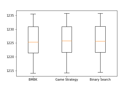
(a) Strong DR-SM NQP

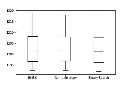
(b) Weak DR-SM NQP

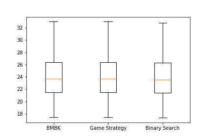
(c) Strong DR-SM Softmax

Figure 2: Box and whisker plots of our experimental results.

5 Conclusion

We proposed a tight approximation algorithm for continuous submodular maximization, and a quasilinear time tight approximation algorithm for the special case of DR-submodular maxmization. Our experiments also verify the applicability of these algorithms in practical domains in machine learning. One interesting avenue for future research is to generalize our techniques to maximization over any arbitrary separable convex set, which would broaden the application domains.

6 Acknowledgments

Rad Niazadeh was supported by Stanford Motwani fellowship. The authors would also like to thank Jan Vondrák for helpful comments and discussions on an earlier draft of this work.

Supplementary Materials

Equivalent definitions of weakly and strongly DR-SM functions.

Proposition 4 ([Bian et al., 2017b]).

Suppose $\mathcal{F}:[0,1]^{n}\rightarrow[0,1]$ is continuous and twice differentiable, and $\mathbf{H}$ is the Hessian of $\mathcal{F}$, i.e. $\forall i,j\in[n],~{}H_{ij}\triangleq\frac{\partial^{2}\mathcal{F}}{\partial{x_{i}}\partial{x_{j}}}$. The followings are equivalent:

1. $\mathcal{F}$ satisfies the weak DR-SM property as in Definition 1.

2. Continuous submodularity: $\forall\textbf{x},\textbf{y}\in[0,1]^{n}$, $\mathcal{F}(\textbf{x})+\mathcal{F}(\textbf{y})\geq\mathcal{F}(\textbf{x}\vee\textbf{y})+\mathcal{F}(\textbf{x}\wedge\textbf{y})$.

3. $\forall i\neq j\in[n],~{}H_{ij}\leq 0$, i.e., all off-diagonal entries of Hessian are non-positive.

Also, the following statements are equivalent:

1. $\mathcal{F}$ satisfies the strong DR-SM property as in Definition 1.

2. $\mathcal{F}(.)$ is coordinate-wise concave along all the coordinates and is continuous submodular, i.e. $\forall\textbf{x},\textbf{y}\in[0,1]^{n}$, $\mathcal{F}(\textbf{x})+\mathcal{F}(\textbf{y})\geq\mathcal{F}(\textbf{x}\vee\textbf{y})+\mathcal{F}(\textbf{x}\wedge\textbf{y})$

3. $\forall i,j\in[n],~{}H_{ij}\leq 0$, i.e., all entries of Hessian are non-positive.

Detailed specifics of experiments in Section 4

Strong-DR Non-concave Quadratic Programming (NQP)

We generated synthetic functions of the form $\mathcal{F}(\textbf{x})=\frac{1}{2}\textbf{x}^{T}\mathbf{H}\textbf{x}+\mathbf{h}^{T}\textbf{x}+c$. We generated $\mathbf{H}\in\mathbb{R}^{n\times n}$ as a matrix with every entry uniformly distributed in $[-1,0]$, and then symmetrized $\mathbf{H}$. We then generated $\mathbf{h}\in\mathbb{R}^{n}$ as a vector with every entry uniformly distributed in $[0,+1]$. Finally, we solved for the value of $c$ to make $\mathcal{F}(\vec{0})+\mathcal{F}(\vec{1})=0$.

Weak-DR Non-concave Quadratic Programming (NQP)

This experiment is the same as in the previous subsection, except that the diagonal entries of $\mathbf{H}$ are uniformly distributed in $[0,+1]$ instead, making the resulting function $\mathcal{F}(\textbf{x})$ only weak DR-SM instead.

Softmax extension of Determinantal Point Processes (DPP)

We generated synthetic functions of the form $\mathcal{F}(\textbf{x})=\log\det(\text{diag}(\textbf{x})(\mathbf{L}-\mathbf{I})+\mathbf{I})$, where $\mathbf{L}$ needs to be positive semidefinite. We generated $\mathbf{L}$ in the following way. First, we generate each of the $n$ eigenvalues by drawing a uniformly random number in $[-0.5,1.0]$ and taking that power of $e$. This yields a diagonal matrix $\mathbf{D}$. We then generate a random unitary matrix $\mathbf{V}$ and then set $\mathbf{L}=\mathbf{V}\mathbf{D}\mathbf{V}^{T}$. By construction, $\mathbf{L}$ is positive semidefinite and has the specified eigenvalues.

More application domain details

Here is a list containing further details about applications in machine learning, electrical engineering and other application domains.

Special Class of Non-Concave Quadratic Programming (NQP).

• The objective is to maximize $\mathcal{F}(\textbf{x})=\frac{1}{2}\textbf{x}^{T}\mathbf{H}\textbf{x}+\mathbf{h}^{T}\textbf{x}+c$, where off-diagonal entries of $\mathbf{H}$ are non-positive (and hence these functions are Weak DR-SM).

• Minimization of this function (or equivalently maximization of this function when off-diagonal entries of $\mathbf{H}$ are non-negative) have been studied in Kim and Kojima [2003] and Luo et al. [2010], and has applications in communication systems and detection in MIMO channels [Luo et al., 2010].

• Another application of quadratic submodular optimization is large-scale price optimization on the basis of demand forecasting models, which has been studied in Ito and Fujimaki [2016]. They show the price optimization problem is indeed an instance of weak-DR minimization.

Revenue Maximization over Social Networks.

• The model was proposed in Bian et al. [2017b] and is a generalization of the revenue maximization problem addressed in Hartline et al. [2008].

• A seller wishes to sell a product to a social network of buyers. We consider restricted seller strategies which freely give (possibly fractional) trial products to buyers: this fractional assignment is our input x of interest.

• The objective takes two effects into account: (i) the revenue gain from buyers who didn’t receive free product, where the revenue function for each such buyer is a nonnegative nondecreasing Weak DR-SM function and (ii) the revenue loss from those who received free product, where the revenue function for each such buyer is a nonpositive nonincreasing Weak DR-SM function. The combination for all buyers is a nonmonotone Weak DR-SM function and additionally is nonnegative at $\vec{0}$ and $\vec{1}$.

Map Inference for Determinantal Point Processes (DPP) & Its Softmax-Extension.

• DPP are probabilistic models that arise in statistical physics and random matrix theory, and their applications in machine learning have been recently explored, e.g. [Kulesza et al., 2012].

• DPPs can be used as generative models in applications such as text summarization, human pose estimation, or news threading tasks [Kulesza et al., 2012].

• A discrete DPP is a distribution over sets, where $p(S)\sim\det(A_{S})$ for a given PSD matrix $A$. The log-likelihood estimation task corresponds to picking a set $\hat{S}\in\mathcal{P}$(feasible set, e.g. a matching) that maximizes $f(S)=\log(\det(A_{S}))$. This function is non-monotone and submodular. Note that as a technical condition to apply bi-greedy algorithms, we require that $\det(A)\geq 1$ (implying $f(\vec{1})\geq 0$).

• The approximation question was studied in [Gillenwater et al., 2012]. Their idea is to first find a fractional solution for a continuous extension (hence a a continuous submodular maximization step is required) and then rounding the solution. However, they sometimes need a fractional solution in $\textrm{conv}(\mathcal{P})$ (so, the optimization task sometimes fall out of the hypercube, making rounding more complicated).

• Beyond multilinear extension, the other continuous extension that has been used in this literature is called the softmax extension [Gillenwater et al., 2012, Bian et al., 2017a]:

  $$\mathcal{F}(\textbf{x})=\log\mathbf{E}_{S\sim\mathcal{I}_{\textbf{x}}}[\exp(f(S))]=\log\det\left(\textrm{diag}(\textbf{x})(A-I)+I\right)$$

  where $\mathcal{I}_{\textbf{x}}$ is the independent distribution with marginals x (i.e. each item $i$ is independently in the set w.p. $x_{i}$).

• $\mathcal{F}(\textbf{x})$ is Strong DR-SM and non-monotone [Bian et al., 2017a]. In almost all machine learning applications, the rounding works on an unrestricted problem. Hence the optimization that needs to be done is Strong DR-SM optimization over unit hypercube.

• One can think of adding a regularizer term $\lambda\lVert\textbf{x}\rVert^{2}$ to the log-likelihood objective function to avoid overfitting. In that case, the underlying fractional problem becomes a Weak DR-SM optimization over the unit hypercube when $\lambda$ is large enough.

Log-Submodularity and Mean-Field Inference.

• Another probabilistic model that generalizes DPP and all other strong Rayleigh measures [Li et al., 2016, Zhang et al., 2015] is the class of log-submodular distributions over sets, i.e. $p(S)\sim\exp(f(S))$ where $f(\cdot)$ is a discrete submodular functions. MAP inference over this distribution has applications in machine learning and beyond [Djolonga and Krause, 2014].

• One variational approach towards this MAP inference task is to do mean-field inference to approximate the distribution $p$ with a product distribution $\textbf{x}\in[0,1]^{n}$, i.e. finding $\textbf{x}^{*}$ that:

  $$\textbf{x}^{*}\in\underset{\textbf{x}\in[0,1]^{n}}{\operatorname{argmax}}~{}~{}\mathbb{H}(\textbf{x})-\mathbf{E}_{S\sim\mathcal{I}_{x}}[\log p(S)]=\underset{\textbf{x}\in[0,1]^{n}}{\operatorname{argmin}}~{}~{}\textrm{KL}(\textbf{x}||p)$$

  where $\textrm{KL}(\textbf{x}||p)=\mathbf{E}_{S\sim\mathcal{I}}[\frac{\log\mathcal{I}_{x}(S)}{\log p(S)}]$.

• The function $\mathcal{F}(\textbf{x})=\mathbb{H}(\textbf{x})-\mathbf{E}_{S\sim\mathcal{I}_{x}}[\log p(S)]$ is Strong DR-SM [Bian et al., 2017a].

Cone Extension of Continuous Submodular Maximization.

• Suppose $\mathcal{K}$ is a proper cone. By considering the lattice corresponding to this cone one can generalize DR submodularity to $\mathcal{K}$-DR submodularity [Bian et al., 2017a].

• An interesting application of this cone generalization is minimizing the loss in the logistic regression model with a particular non-separable and non-convex regularizer, as described in [Antoniadis et al., 2011, Bian et al., 2017a]. Bian et al. [2017a] show the vanilla version is a $\mathcal{K}$-Strong DR-SM function maximization for some particular cone.

• Note that by adding a $\mathcal{K}$-$\ell_{2}$-norm regularizer $\lambda\lVert\textbf{A}\textbf{x}\rVert^{2}$, the function will become Weak DR-SM, where A is a matrix with generators of $\mathcal{K}$ as its column. Here is the logistic loss:

  $$l(\textbf{x},\{y_{t}\})=\frac{1}{T}\sum_{t=1}^{T}f_{t}(\textbf{x},y_{t})=\frac{1}{T}\sum_{t=1}^{T}\log(1+\exp(-y_{t}\textbf{x}^{T}\mathbf{z}^{t}))$$

  where $y_{t}$ is the label of the $t^{\textrm{th}}$ data-point, x are the model parameters, and $\{\mathbf{z}^{t}\}$ are feature vectors of the data-points.

Remark 1.

In many machine learning applications, and in particular MAP inference of DPPs and log-submodular distributions, unless we impose some technical assumptions, the underlying Strong DR-SM (or Weak DR-SM) function is not necessarily positive (or may not even satisfy the weaker yet sufficient condition $\mathcal{F}(\vec{0})+\mathcal{F}(\vec{1})\geq 0$). In those cases, adding a positive constant to the function can fix the issue, but the multiplicative approximation guarantee becomes weaker. However, this trick tends to work in practice since these algorithms tend to be near optimal.

References

• Antoniadis et al. [2011] Anestis Antoniadis, Irène Gijbels, and Mila Nikolova. Penalized likelihood regression for generalized linear models with non-quadratic penalties. Annals of the Institute of Statistical Mathematics, 63(3):585–615, 2011.
• Bach et al. [2013] Francis Bach et al. Learning with submodular functions: A convex optimization perspective. Foundations and Trends® in Machine Learning, 6(2-3):145–373, 2013.
• Bian et al. [2017a] An Bian, Kfir Levy, Andreas Krause, and Joachim M Buhmann. Continuous DR-submodular maximization: Structure and algorithms. In Advances in Neural Information Processing Systems, pages 486–496, 2017a.
• Bian et al. [2017b] Andrew An Bian, Baharan Mirzasoleiman, Joachim Buhmann, and Andreas Krause. Guaranteed non-convex optimization: Submodular maximization over continuous domains. In Artificial Intelligence and Statistics, pages 111–120, 2017b.