Input and Weight Space Smoothing for Semi-supervised Learning

Abstract

We propose regularizing the empirical loss for semi-supervised learning by acting on both the input (data) space, and the weight (parameter) space. We show that the two are not equivalent, and in fact are complementary, one affecting the minimality of the resulting representation, the other insensitivity to nuisance variability. We propose a method to perform such smoothing, which combines known input-space smoothing with a novel weight-space smoothing, based on a min-max (adversarial) optimization. The resulting Adversarial Block Coordinate Descent (ABCD) algorithm performs gradient ascent with a small learning rate for a random subset of the weights, and standard gradient descent on the remaining weights in the same mini-batch. It achieves comparable performance to the state-of-the-art without resorting to heavy data augmentation, using a relatively simple architecture.

1 Introduction

In semi-supervised learning, we are given $N^{l}$ labeled samples $x^{l}\in X^{l}$ with corresponding labels $y^{l}\in Y^{l}$ and $N^{u}$ unlabeled samples, $x^{u}\in X^{u}$. The entire training dataset is $X$ with cardinality $N=N^{l}+N^{u}$. For a discriminative model to exploit unlabeled data, there has to be some prior on the model parameters or on the unknown labels (Chapelle et al., (2009)). Such a prior can be realized through a regularization functional acting on either the parameters (weight space) or the data (input space). Both input-space regularization, or “smoothing” (Joachims, (1999); Goodfellow et al., 2014a ; Miyato et al., (2017)) and weight-space smoothing (Hochreiter and Schmidhuber, (1997); Chaudhari et al., (2016)) have been shown to improve both supervised (SL) and semi-supervised learning (SSL). The first question we address is whether the two are, in some sense, equivalent.

To answer the question, we conduct experiments that show that, for nonlinear and/or over-parametrized classifiers, input and weight smoothing are not only not equivalent, but they are complementary, suggesting that applying both may be beneficial. The second question we address, therefore, is whether this can be done efficiently and yield performance improvements relative to methods that only smooth one of the two.

To address this, we propose a new algorithm for weight smoothing called Adversarial Block Coordinate Descent (ABCD), which we combine with a standard input-smoothing algorithm (VAT), and test the result on SSL benchmarks on the CIFAR10 and SVHN benchmark datasets. ABCD combined with VAT achieves state-of-the-art performance with minimal data augmentation (translation and reflection), without complex architectures (e.g. ResNet) and no sophisticated learning machinery.

While in this section our method is motivated heuristically, there are theoretical groundings for performing joint regularization in weight- and input-space, which we discuss in the Supplementary Material. In the next two subsections we describe input and weight smoothing, and in the following subsection we show them to not be equivalent. In the next section we describe the proposed algorithm ABCD, and in the following one we put it to the test on SSL benchmarks.

1.1 Input smoothing

We call a classifier “input smooth" when its predictions are robust to small perturbations in the input space. So, input smoothing can be obtained with the following optimization problem:

$$\min_{w} \ \sum_{x_{i}\in X}\ell(f(x_{i};w),f(x_{i}+\Delta x_{i};w))$$

$${\rm subject\ to} \ \Delta x_{i}=\operatorname*{arg\;max}_{||\Delta x_{i}||<\epsilon_{x}}\ell(f(x_{i};w),f(x_{i}+\Delta x_{i};w))\,\forall x_{i}\in X$$ (1)

where $\ell()$ can be cross-entropy, Kullbach-Liebler (KL) divergence or the mean-square error. $f(x;w)\in\mathbb{R}^{K}$ is the network output with weights $w$ and $K$ is the number of classes. This problem can be solved along with minimizing the objective function designed for the task, for instance the cross-entropy loss for classification. In other words, a desirable classifier should not change its predictions for any additive perturbation within a ball of small radius $\epsilon_{x}$ for any input $x_{i}$. This idea is also known as max-margin or low-density assumptions in the SSL literature, championed by TSVM (Joachims, (1999)). Although the perturbations to which we seek insensitivity are unstructured, in imaging data the largest perturbations are often due to nuisance variability (e.g.. changes in illumination, vantage point, or visibility).

A popular way of attacking to this min-max problem is through the use of adversarial examples. The underlying idea is to add a (regularization) term to the loss function, that penalizes the difference between network outputs for clean samples, and samples with added adversarial noise. Adversarial training (Goodfellow et al., 2014a ) applies this idea to supervised learning where they change the problem to being robust against noise by moving predictions away from the ground truth labels:

$$\min_{w} \ \sum_{x_{i}\in X}\ell(f(x_{i};w),f(x_{i}+\Delta x_{i};w))$$

$${\rm subject\ to} \ \Delta x_{i}=\operatorname*{arg\;max}_{||\Delta x_{i}||<\epsilon_{x}}\ell(P(y_{i}|x_{i}),f(x_{i}+\Delta x_{i};w))\,\forall x_{i}\in X$$ (2)

For this supervised setting, ground truth labels $P(y|x)$ can be used in calculating the adversarial noise $\Delta x$. Instead of finding the exact $\Delta x$ for each input $x$, Goodfellow et al., 2014a calculates the first order approximation of adversarial perturbation leading to maximum change in the classifier predictions $f(x;w)$:

$$\Delta x\approx\epsilon_{x}\frac{g}{||g||_{2}}$$

$${\rm subject\ to} \ g=\nabla_{x}\ell(P(y|x),f(x;w))$$ (3)

where $P(y|x)$ is the ground truth label for sample $x$. A natural extension of this idea to SSL is introduced by Miyato et al., (2015, 2017). Since SSL algorithms do not have access to ground truth labels $P(y|x)$, their adversarial noise attempts to maximize $\ell(f(x;w),f(x+\Delta x;w))$. But, in the SSL case, the first-order approximation is not useful, because the first derivative of $\ell(f(x;w),f(x+\Delta x;w))$ is always zero at $\Delta x=0$. Hence, Miyato et al., (2015, 2017) make a second-order approximation for $\Delta x$ and propose the following approximation to the adversarial noise for each input $x$:

$$\Delta x\approx\epsilon_{x}\frac{g}{||g||_{2}}$$

$${\rm subject\ to} \ g=\nabla_{\Delta x}\ell(f(x;w),f(x+\Delta x;w))\Big{|}_{\Delta x=\xi d}$$ (4)

where $d\sim N(0,1)$. Therefore, the regularization loss of Miyato et al., (2015, 2017) is

$$\ell_{VAT}(x;w):=\ell(f(x;w),f(x+\epsilon_{x}\frac{g}{||g||_{2}};w))$$

$${\rm subject\ to} \ g=\nabla_{\Delta x}\ell(f(x;w),f(x+\Delta x;w))\Big{|}_{\Delta x=\xi d}$$ (5)

for one input sample $x$. We will minimize this regularizer as a way of doing input smoothing in our final SSL algorithm.

1.2 Weight smoothing

Just like the input smoothing, weight smoothing can be formulated as a min-max problem. More explicitly,

$$\min_{w} \ \sum_{x_{i}\in X}\ell(f(x_{i};w),f(x_{i};w+\Delta w))$$

$${\rm subject\ to} \ \Delta w=\operatorname*{arg\;max}_{||\Delta w||<\epsilon_{w}}\sum_{x_{i}\in X}\ell(f(x_{i};w),f(x_{i};w+\Delta w))$$ (6)

Unlike input smoothing, the parameters of both minimization and maximization are the same, namely the weights of the network, $w$. It is important to note that maximum is taken within a ball of small radius $\epsilon_{w}$. This appears counter-intuitive at first.

Just like input smoothing can be associated with insensitivity to nuisance variability in the data (hence bias the representation towards invariance), weight smoothing can be associated with generalization, as it has been observed empirically that so-called “flat-minima” (Hochreiter and Schmidhuber,, 1997; Jastrzębski et al.,, 2017) corresponds to solutions that tend to yield better generalization. Recent methods (Chaudhari et al.,, 2016) try to bias solutions towards such flat minima, including using a conservative penalty (Li et al.,, 2014):

$$w_{t}=\operatorname*{arg\;min}_{w}\ell(P(y|x);f(x;w))+\gamma||w-w_{t-1}||^{2}_{2}.$$ (7)

We follow a related, but different, approach: We explicitly find adversarial directions with respect to random subsets of the weights, then force the network to be robust against these directed perturbation using the remaining weights.

This problem of optimizing for the worst case is also studied in the robust optimization literature (Bertsimas et al.,, 2010). Given “all” the possible adversarial $\Delta w$ values maximizing the loss, they suggest an optimization framework for finding descent directions with second-order cone programming (SOCP) which would guarantee an optimal solution for a convex objective. Since finding all possible adversarial perturbations is not feasible, they find the ones around a ball with gradient ascent and solve SOCP for local solutions iteratively, which is related to our method.

1.3 Input smoothing and weight smoothing do not imply each other

Figure 1: Over-parametrized networks are more robust to adversarial noises in the weight space even when they have the same decision boundary (i.e. the same input smoothness). Three MLP networks with different number of hidden units trained with VAT on the half-moon dataset (first panel) have the same decision boundary (second panel). Moreover, the network response (probability given to one of the classes) is almost the identical for each of three networks (third panel). Therefore, robustness of the networks to input perturbation is not just same in “error" sense but also same in “loss" sense. However, the larger the network gets, the more robust it is to the adversarial perturbations in the weight space. Fourth panel shows the training loss versus number of gradient ascent directions for varying sized networks. As it can be seen, having a visible increase in the loss takes more ascent steps for larger networks. This experiment illustrates that networks with the same robustness to input perturbations may have completely different sensitivities to perturbations in the weight space.

For a linear classifier, the Hessian of the mean-square error (MSE) loss is the data covariance matrix. The local geometry of the loss landscape around the solution where the weights converged does not depend on the classifier structure, nor on its parametrization. The number of zero eigenvalues is determined by the dimensionality of the input data matrix alone. However, it can be easily shown that this is not necessarily the case for nonlinear classifiers. For instance, Sagun et al., (2017) shows that the number of zero eigenvalues of the approximate Hessian of the loss has a lower bound of $|w|-N$, where $N$ is the number of training samples and $|w|$ is the number of weights. This simple Hessian argument suggests that the robustness of a network to weight perturbations depends on factors other than its robustness to input perturbations, like the number of parameters in the network, for nonlinear classifiers. Even though they also have empirical evidence for this claim, the spectrum of the Hessian alone is not necessarily a good measure of flatness (Dinh et al.,, 2017). So, we construct a toy experiment to verify that input smoothness does not necessarily imply weight smoothness.

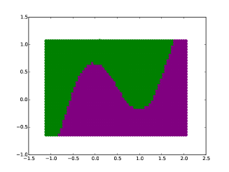
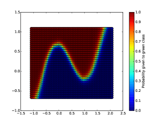
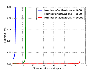
We use a half-moon toy dataset whereby there are $4$ labeled (larger circles) and $1000$ unlabeled samples from each cluster (first panel of Fig. 1). We run the VAT algorithm to find the max-margin decision boundary (second panel of Fig. 1). We repeat this experiment for 3 multi-layer perceptron (MLP) networks each having the same structure, except for a different number of weights. The decision boundary is the same, as it can be seen in the second panel of Fig. 1, where they show as one as they overlap perfectly. This implies that for any perturbation in the input space, the increase in the error would be the same for each of these classifiers. To show that this also the case for the loss, we also provide the network response and again they are indistinguishable (third panel of Fig. 1). Hence, input smoothness is the same for each of three MLPs.

After training three MLP networks with VAT, we apply gradient ascent on the converged weights with a small learning rate to evaluate the robustness of the networks with different number of weights. As it can be seen in the right panel of Fig. 1, it takes more ascent updates for large networks to diverge. Thus, over-parametrized networks are more robust to perturbations in weight space. This experiment shows that input smoothing does not necessarily imply weight smoothing. I.e. there are factors other than input smoothness determining the geometry of the loss around the converged weight. Another observation is that losses diverge suddenly, implying that it takes several iterations to increase the loss, during which time the landscape is almost constant, before the loss increases sharply. The ascent learning rate chosen in the experiment is $0.005$. During ascent, SGD without momentum and weight decay is used. MLPs are in the form $2\rightarrow FC(n)\rightarrow FC(n)\rightarrow FC(n)\rightarrow FC(n)\rightarrow 2$ where $FC(n)$ is fully connected layer followed by a RELU and $n$ is number of hidden units. We report results for $n=1000$, $n=2500$ and $n=10000$.

Note that we choose to make our experiments in two dimensional inputs to visualize the decision boundary easily and verify that they are the same for different classifiers; not because these results are restricted to small dimensional inputs. These results align with those of Freeman and Bruna, (2016) where they suggest that the amount of uphill climbing for connecting arbitrary weight pairs is correlated to the size of the network. For more discussion on the effect of over-parametrization on the loss landscape of DNNs see Safran and Shamir, (2016); Sagun et al., (2014); Baity-Jesi et al., (2018); Soudry and Carmon, (2016).

1.4 Joint input and weight smoothing

Once established that input smoothness and weight smoothness are not equivalent, it is natural to try enforcing both. So, the additional regularization we want to have can be framed as follows:

$$\min_{w} \ \sum_{x_{i}\in X}\ell(f(x_{i};w),f(x_{i};w+\Delta w))+\ell(f(x_{i};w),f(x_{i}+\Delta x_{i};w))$$

$${\rm subject\ to} \ \Delta w=\operatorname*{arg\;max}_{||\Delta w||<\epsilon_{w}}\sum_{x_{i}\in X}\ell(f(x_{i};w),f(x_{i};w+\Delta w))$$

$$\ \Delta x_{i}=\operatorname*{arg\;max}_{||\Delta x_{i}||<\epsilon_{x}}\ell(f(x_{i};w),f(x_{i}+\Delta x_{i};w))\,\forall x_{i}\in X$$ (8)

So, the regularization term we want to minimize for one input $x$ is

$$L(x;w)=\ell(f(x;w),f(x;w+\operatorname*{arg\;max}_{||\Delta w||<\epsilon_{w}}\sum_{x_{i}\in X}\ell(f(x_{i};w),f(x_{i};w+\Delta w))))+$$

$$\ell(f(x;w),f(x+\operatorname*{arg\;max}_{||\Delta x||<\epsilon_{x}}\ell(f(x;w),f(x+\Delta x;w));w))$$ (9)

Then, the overall problem we want to solve in the supervised learning setting becomes

$$\min_{w} \ \sum_{x}\ell_{CE}(x;w)+\lambda L(x;w)$$ (10)

where

$$\ell_{CE}(x;w)=-\langle P(y|x),\log f(x;w)\rangle$$ (11)

is the cross entropy loss calculated for label estimates $f(x;w)$ and ground truth labels $P(y|x)$.

Calculating the exact $\Delta x$ for each input is not trivial. Instead, we will use VAT in Eq. 4 to make our classifier robust against input space perturbations. For achieving weight space smoothness, we will use the proposed algorithm described next.

2 Adversarial Block Coordinate Descent (ABCD)

Algorithm 1 Adversarial Block Coordinate Descent (ABCD)

1:Input: Minibatch set $B_{t}$, loss function $\ell(\cdot)$, initial weights $w_{0}$.

2:Hyper-parameters: Ascent and descent learning rates $\eta_{A}$ and $\eta_{D}$. Number of inner iterations $L$.

3:Output: Final weights $w_{L}$.

4:for $l=1:L$ do

5:     $\Gamma_{i}$ sample from $\{0,-1\}$ for all $i\in\{1,\ldots,|w_{0}|\}$.

6:     $\Gamma^{a}_{i}=\Gamma_{i}$ for all $i\in\{1,\ldots,|w_{0}|\}$.

7:     $\Gamma^{d}_{i}=\Gamma_{i}+1$ for all $i\in\{1,\ldots,|w_{0}|\}$.

8:     // Run stochastic gradient ascent with a small learning rate $\eta_{A}$

9:     $w_{l-\frac{1}{2}}=w_{l-1}-\eta_{A}\Gamma^{a}\odot\nabla_{w_{l-1}}\left(\frac{1}{|B_{t}|}\sum_{i=1}^{|B_{t}|}\ell(x_{i};w_{l-1})\right)$

10:     // Run stochastic gradient descent with a learning rate $\eta_{D}\gg\eta_{A}$

11:     $w_{l}=w_{l-\frac{1}{2}}-\eta_{D}\Gamma^{d}\odot\nabla_{w_{l-\frac{1}{2}}}\left(\frac{1}{|B_{t}|}\sum_{i=1}^{|B_{t}|}\ell(x_{i};w_{l-\frac{1}{2}})\right)$

Since the parameters of both minimization and maximization are the weights of the network for the min-max problem in Eq. (6), we use a subset of the weights $w$ for finding adversarial directions in weight space and the rest to impose robust to such additive adversarial perturbations in weight space. For this, at each update, we randomly choose half of the weights and take a gradient ascent step along them with a small learning rate. Then, on the same batch, we apply gradient descent for the remaining weights with ordinary (larger) learning rate. We call this algorithm Adversarial Block Coordinate Descent (ABCD), for pseudo-code, see Alg. 1. ABCD can be considered as an extension of Dropout (Hinton et al.,, 2012; Srivastava et al.,, 2014) and coordinate descent (Wright,, 2015). However, unlike Dropout, we explicitly regularize our network to be robust against “adversarial directions" in the weight space; instead of just being robust to zeroed out weights.

Algorithm 2 SSL algorithm using ABCD as optimizer; VAT and entropy as regularizers. $\ell_{CE}(x;w)$, $\ell_{E}(x;w)$, $\ell_{VAT}(x;w)$ are as defined in Eq. 11, Eq. 12, Eq. 5 respectively.

1:for $t=1:T$ do

2:     // Run ABCD on cross entropy for labeled samples:

3:     Sample $B^{l}_{t}$

4:     $w_{t^{\prime}}=ABCD(B^{l}_{t},\ell_{CE}(x;w),w_{t-1})$ // weight smoothing

5:     // Run ABCD on entropy and SGD on VAT loss for unlabeled samples:

6:     Sample $B^{u}_{t}$

7:     $w_{t^{\prime}}=ABCD(B^{u}_{t},\ell_{E}(x;w),w_{t^{\prime}})$ // weight smoothing

8:     $w_{t}=SGD(B^{u}_{t},\ell_{VAT}(x;w),w_{t^{\prime}})$ // input smoothing

The randomness in ABCD are due to mini-batch optimization that we have to use for computational reasons and the randomness in the mask $\Gamma$ selection. If we ignore these, it would be easier to see the loss minimized by ABCD. The loss minimized by descent in ABCD is the “worst case” of the nominal loss landscape. By worst case we mean that, at each point in the weight space, the loss ABCD minimizes is the maximum that can be reached from that point with one small ascent step. In other words, ABCD minimizes the maximum loss around a small ball at each point. Moreover, we do not want the last update for any of the weight parameter to be ascent. So, we do not apply ABCD in the last few epochs.

ABCD can be used for SSL in place of vanilla SGD. We use ABCD for SSL by minimizing the empirical cross entropy for labeled data and the entropy of empirical estimates for the unlabeled data with ABCD. That is,

$$\ell_{E}(x;w)=-\langle f(x;w),\log f(x;w)\rangle$$ (12)

for unlabeled data which is a well-known regularizer in the SSL literature (Dai et al.,, 2017; Grandvalet and Bengio,, 2005; Krause et al.,, 2010; Springenberg,, 2015).

We additionally report performance of ABCD combined with VAT to see the effect of applying both input and weight smoothing. The pseudo-code using VAT as loss function and ABCD as optimizer for SSL task is given in Alg. 2. For labeled data, ABCD used as an optimizer to minimize cross entropy to achieve weight smoothing. We do not minimize $\ell_{VAT}(x;w)$ for labeled data as proposed in the corresponding paper. For unlabeled data, ABCD is used to minimize entropy $\ell_{E}(x;w)$ and SGD is used to minimize $\ell_{VAT}(x;w)$ for weight and input smoothing respectively. We set $\eta_{A}=10^{-5}$ for all of our experiments. $\eta_{D}$ can be chosen as usual with high initial value from $\{0.1,0.01\}$ and is decreased during training. In all the SSL experiments, we only use the network called conv-large from Miyato et al., (2017); Tarvainen and Valpola, (2017). Only translation and horizontal flipping are used as data augmentations to allow fair comparison with some of the previous SSL algorithms. Horizontal flipping is only used in CIFAR10.

In our implementation of VAT (Miyato et al.,, 2017), we set $\epsilon_{x}$ in Eq. 4 to be $128$ for CIFAR10 and $0.25$ for SVHN. Even though we search $\epsilon_{x}$ in a fine grid, we could not get to the performance reported in their paper for CIFAR10; possibly because we use a different optimizer (SGD instead of ADAM), different learning rate scheme and different ZCA regularizer. The performance of our VAT implementation is given in Table 1. Our implementation ($13.28\%$) of VAT without entropy minimization is about $2$ percent worse than what is reported in Miyato et al., (2017) ($11.36\%$) for CIFAR10. But, we still use the numbers reported in Miyato et al., (2017) for comparison purposes in Table 1. Additional details on training given in the Supplementary Material.

3 Evaluation

Figure 2: Robustness of ABCD vs SGD trained networks to ascent updates. Starting from the ABCD and SGD trained weights, we apply gradient ascent with learning rate $0.001$ on the cross entropy loss. This plot shows the increase in the training loss versus number of ascent steps. Both weights diverge quickly, but ABCD trained network diverges later than that of SGD verifying the robustness of ABCD to weight space perturbations. 1D visualization of loss landscapes of SGD and ABCD trained weights. Training and test losses over the curve $\alpha*w_{SGD}+(1-\alpha)*w_{ABCD}$ are given as suggested by Goodfellow et al., 2014b where $\alpha\in[-0.2,1.2]$. $\alpha=0$ and $\alpha=1$ correspond to the weights of ABCD and SGD trained networks respectively. This method compares the flatness of two methods in one direction only and in that direction, ABCD seems much more robust to weight perturbations.

SSL Method	Test error rate (%)
	CIFAR10	SVHN
	$N^{l}=4,000$	$N^{l}=1,000$
	$N^{u}=46,000$	$N^{u}=72,257$
VAT+EntMin Miyato et al., (2017)	$10.55$	$3.86$
Stochastic Transformation Sajjadi et al., (2016)	$11.29$	NR
Temporal Ensemble Laine and Aila, (2016)	$12.16$	$4.42$
GAN+FM Salimans et al., (2016)	$15.59$	$5.88$
Mean Teacher Tarvainen and Valpola, (2017)	$12.31$	$3.95$
EntMin (our implementation)	$15.42$ $\pm$ $0.22$	$6.02$ $\pm$ $0.02$
VAT without EntMin (our implementation)	$13.28$ $\pm$ $0.11$	$5.60$ $\pm$ $0.29$
VAT+EntMin (our implementation)	$11.81$ $\pm$ $0.07$	$4.10$ $\pm$ $0.06$
ABCD+EntMin	$11.98$ $\pm$ $0.04$	$4.93$ $\pm$ $0.04$
ABCD+EntMin+VAT	$10.11$ $\pm$ $0.14$	$3.63$ $\pm$ $0.03$

Table 1: Comparison with the state-of-the-art on SSL tasks. Error rates on the test set are given for CIFAR10 and SVHN. NR stands for “not reported.” CIFAR10 is trained using 4,000 labeled and 46,000 unlabeled samples, SVHN using 1,000 labeled and 72,257 unlabeled samples. Results are averaged over three random labeled sets. We report performance of ABCD alone and combined with VAT. ABCD+EntMin+VAT refers to algorithm in Alg. 2 where ABCD is used as an optimizer; entropy and VAT are used as regularizers in the loss function. ABCD+EntMin uses only entropy for unlabeled data to report performance of ABCD without VAT. SSL baselines. Baseline algorithms are EntMin, VAT and VAT+EntMin. EntMin minimizes the entropy of estimates for unlabeled data with standard SGD. Similarly, VAT minimizes $\ell_{VAT}$ from Eq. 5 and VAT+EntMin minimizes both on unlabeled data. Note that these are the results we get with our own implementation of VAT.

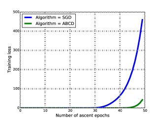
To evaluate the robustness of ABCD-trained weights to adversarial weight space perturbations, we report the number of ascent updates necessary for the loss to diverge. In Fig. 2 (left), the plot of training loss v.s. number of ascent updates is given for SGD and ABCD-trained weights. As it can be seen, the number of ascent updates needed for the loss to diverge for ABCD is more than for SGD.

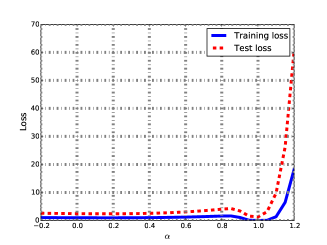
Another way of comparing the local geometrical properties of the weights is by visualizing the loss landscape around the converged weights. As the deep networks we use have very high dimension, several visualization tricks have been suggested to visualize the loss landscapes in $1$- or $2$-dimensional subsets of the weight space (Li et al.,, 2017; Goodfellow et al., 2014b, ; Keskar et al.,, 2016). We employ the technique suggested in Goodfellow et al., 2014b in Fig. 2 (right): we plot the loss on the curve $\alpha*w_{SGD}+(1-\alpha)*w_{ABCD}$ where $\alpha\in[-0.2,1.2]$. $w_{SGD}$ and $w_{ABCD}$ are the weights converged when training with SGD and ABCD respectively. As it can be seen, the loss does not increase around ABCD trained weights. We also report Hessian histograms in the Supplementary Material. Further details on the networks and datasets used in the experiments given there.

In Table 1, we compare the performance of ABCD with state-of-the-art SSL algorithms. We report performance of the proposed algorithm on SVHN (Netzer et al.,, 2011) and CIFAR10 (Krizhevsky and Hinton,, 2009) in SSL setting. SVHN consists of $32\times 32$ images of house numbers. We use $73,257$ samples for training, rather than the entire $600,000$ images; $26,032$ images are separated for evaluation. CIFAR10 has $60,000$ $32\times 32$ images, of which $50,000$ are used for training and $10,000$ for testing. We choose labeled samples randomly. We also choose them to be uniform over the classes as it is done in previous works (Miyato et al.,, 2017). In CIFAR10, $4,000$ and in SVHN $1,000$ of training samples are labeled. Except Sajjadi et al., (2016), all the methods use modest augmentations (translation and horizontal flipping) and do not exploit recent deep learning models like ResNet (He et al.,, 2016). We report ABCD with entropy minimization alone and combined with VAT. When we run ABCD only with entropy minimization, it yields second-best SSL performance after VAT in CIFAR10 excluding Sajjadi et al., (2016). Combining ABCD with VAT improves the scores verifying that they are complementary.

4 Discussion and Related Work

Next, we discuss our contribution in the context of related and recent work in SSL.

Input smoothing in SSL. In addition to work referenced earlier, there are graph-based methods (Solomon et al.,, 2014; Yang et al.,, 2016) that penalize having different labels for similar input pairs. For instance, given that $s_{ij}$ is the measure of similarity for input samples $x_{i}$ and $x_{j}$, they minimize the energy $s_{ij}(f(x_{i};w)-f(x_{j};w))^{2}$ performing label propagation under the constraint of fitting to labeled data. This forces the discriminant to change little in response to different inputs with large $s_{ij}$. Generative models by Springenberg, (2015) suggests that they maximize the margin with the help of fake samples.

Weight smoothing in SSL. Teacher-student methods (Laine and Aila,, 2016; Tarvainen and Valpola,, 2017) average over many predictions or weights in a way that the teacher network can attract student networks towards itself. A similar algorithm is suggested by Zhang et al., (2015) for parallel computing under communication constraint where each replica is attracted to the reference system. Baldassi et al., (2016) studies such algorithms for models with discrete variables and they argue that they achieve to find robust local minimas. Thus, one can relate the success of teacher-student models of state-of-the-art deep SSL algorithms for their ability to converge to robust weights. We recently became aware that Park et al., (2017) also combine VAT with Virtual Adversarial Dropout (VAdD) and, like us, improve upon the VAT baseline as a result. VAdD finds a zero mask of dropout adversarially at each update rather than trying to be robust against adversarial “directions". We find the latter approach more effective in achieving weight smoothing and avoiding convergence to locations in the loss landscape with strong ascent directions. As a result, we reach comparable performance to Park et al., (2017) without using sophisticated rate scheduling like ramp-up and mean-only batch-normalization (Salimans and Kingma,, 2016).

Effect of noise to generalization. Adding random noise to gradients is known to improve the generalization (Welling and Teh,, 2011). Jastrzębski et al., (2017) analyzes the effect of the inherent noise due mini-batch usage in the properties of point converged by SGD. They conclude that for larger noise, network favors wider minima more under the assumption that the noise is isotropic. ABCD differs from these works by adding adversarial noise to weights instead of random noise.

Acknowledgments

SC would like to thank Pratik Chaudhari for fruitful discussions and valuable suggestions.

References

- Baity-Jesi et al., (2018) Baity-Jesi, M., Sagun, L., Geiger, M., Spigler, S., Arous, G. B., Cammarota, C., LeCun, Y., Wyart, M., and Biroli, G. (2018). Comparing dynamics: Deep neural networks versus glassy systems. arXiv preprint arXiv:1803.06969.
- Baldassi et al., (2016) Baldassi, C., Borgs, C., Chayes, J. T., Ingrosso, A., Lucibello, C., Saglietti, L., and Zecchina, R. (2016). Unreasonable effectiveness of learning neural networks: From accessible states and robust ensembles to basic algorithmic schemes. Proceedings of the National Academy of Sciences, 113(48):E7655–E7662.
- Bertsimas et al., (2010) Bertsimas, D., Nohadani, O., and Teo, K. M. (2010). Robust optimization for unconstrained simulation-based problems. Operations research, 58(1):161–178.
- Chapelle et al., (2009) Chapelle, O., Scholkopf, B., and Zien, A. (2009). Semi-supervised learning (chapelle, o. et al., eds.; 2006)[book reviews]. IEEE Transactions on Neural Networks, 20(3):542–542.
- Chaudhari et al., (2016) Chaudhari, P., Choromanska, A., Soatto, S., and LeCun, Y. (2016). Entropy-sgd: Biasing gradient descent into wide valleys. arXiv preprint arXiv:1611.01838.
- Cicek et al., (2018) Cicek, S., Fawzi, A., and Soatto, S. (2018). Saas: Speed as a supervisor for semi-supervised learning. arXiv preprint arXiv:1805.00980.
- Dai et al., (2017) Dai, Z., Yang, Z., Yang, F., Cohen, W. W., and Salakhutdinov, R. (2017). Good semi-supervised learning that requires a bad gan. arXiv preprint arXiv:1705.09783.
- Dinh et al., (2017) Dinh, L., Pascanu, R., Bengio, S., and Bengio, Y. (2017). Sharp minima can generalize for deep nets. arXiv preprint arXiv:1703.04933.
- Freeman and Bruna, (2016) Freeman, C. D. and Bruna, J. (2016). Topology and geometry of half-rectified network optimization. arXiv preprint arXiv:1611.01540.
- (10) Goodfellow, I. J., Shlens, J., and Szegedy, C. (2014a). Explaining and harnessing adversarial examples. arXiv preprint arXiv:1412.6572.
- (11) Goodfellow, I. J., Vinyals, O., and Saxe, A. M. (2014b). Qualitatively characterizing neural network optimization problems. arXiv preprint arXiv:1412.6544.
- Grandvalet and Bengio, (2005) Grandvalet, Y. and Bengio, Y. (2005). Semi-supervised learning by entropy minimization. In Advances in neural information processing systems, pages 529–536.
- He et al., (2016) He, K., Zhang, X., Ren, S., and Sun, J. (2016). Deep residual learning for image recognition. In Proceedings of the IEEE conference on computer vision and pattern recognition, pages 770–778.
- Hinton et al., (2012) Hinton, G. E., Srivastava, N., Krizhevsky, A., Sutskever, I., and Salakhutdinov, R. R. (2012). Improving neural networks by preventing co-adaptation of feature detectors. arXiv preprint arXiv:1207.0580.
- Hochreiter and Schmidhuber, (1997) Hochreiter, S. and Schmidhuber, J. (1997). Flat minima. Neural Computation, 9(1):1–42.
- Jastrzębski et al., (2017) Jastrzębski, S., Kenton, Z., Arpit, D., Ballas, N., Fischer, A., Bengio, Y., and Storkey, A. (2017). Three factors influencing minima in sgd. arXiv preprint arXiv:1711.04623.
- Joachims, (1999) Joachims, T. (1999). Transductive inference for text classification using support vector machines. In ICML, volume 99, pages 200–209.
- Keskar et al., (2016) Keskar, N. S., Mudigere, D., Nocedal, J., Smelyanskiy, M., and Tang, P. T. P. (2016). On large-batch training for deep learning: Generalization gap and sharp minima. arXiv preprint arXiv:1609.04836.
- Krause et al., (2010) Krause, A., Perona, P., and Gomes, R. G. (2010). Discriminative clustering by regularized information maximization. In Advances in neural information processing systems, pages 775–783.
- Krizhevsky and Hinton, (2009) Krizhevsky, A. and Hinton, G. (2009). Learning multiple layers of features from tiny images.
- Laine and Aila, (2016) Laine, S. and Aila, T. (2016). Temporal ensembling for semi-supervised learning. arXiv preprint arXiv:1610.02242.
- Li et al., (2017) Li, H., Xu, Z., Taylor, G., and Goldstein, T. (2017). Visualizing the loss landscape of neural nets. arXiv preprint arXiv:1712.09913.
- Li et al., (2014) Li, M., Zhang, T., Chen, Y., and Smola, A. J. (2014). Efficient mini-batch training for stochastic optimization. In Proceedings of the 20th ACM SIGKDD international conference on Knowledge discovery and data mining, pages 661–670. ACM.
- Miyato et al., (2017) Miyato, T., Maeda, S.-i., Koyama, M., and Ishii, S. (2017). Virtual adversarial training: a regularization method for supervised and semi-supervised learning. arXiv preprint arXiv:1704.03976.
- Miyato et al., (2015) Miyato, T., Maeda, S.-i., Koyama, M., Nakae, K., and Ishii, S. (2015). Distributional smoothing with virtual adversarial training. arXiv preprint arXiv:1507.00677.
- Netzer et al., (2011) Netzer, Y., Wang, T., Coates, A., Bissacco, A., Wu, B., and Ng, A. Y. (2011). Reading digits in natural images with unsupervised feature learning. In NIPS workshop on deep learning and unsupervised feature learning, volume 2011, page 5.
- Park et al., (2017) Park, S., Park, J.-K., Shin, S.-J., and Moon, I.-C. (2017). Adversarial dropout for supervised and semi-supervised learning. arXiv preprint arXiv:1707.03631.
- Safran and Shamir, (2016) Safran, I. and Shamir, O. (2016). On the quality of the initial basin in overspecified neural networks. In International Conference on Machine Learning, pages 774–782.
- Sagun et al., (2017) Sagun, L., Evci, U., Guney, V. U., Dauphin, Y., and Bottou, L. (2017). Empirical analysis of the hessian of over-parametrized neural networks. arXiv preprint arXiv:1706.04454.
- Sagun et al., (2014) Sagun, L., Guney, V. U., Arous, G. B., and LeCun, Y. (2014). Explorations on high dimensional landscapes. arXiv preprint arXiv:1412.6615.
- Sajjadi et al., (2016) Sajjadi, M., Javanmardi, M., and Tasdizen, T. (2016). Regularization with stochastic transformations and perturbations for deep semi-supervised learning. In Advances in Neural Information Processing Systems, pages 1163–1171.
- Salimans et al., (2016) Salimans, T., Goodfellow, I., Zaremba, W., Cheung, V., Radford, A., and Chen, X. (2016). Improved techniques for training gans. In Advances in Neural Information Processing Systems, pages 2234–2242.
- Salimans and Kingma, (2016) Salimans, T. and Kingma, D. P. (2016). Weight normalization: A simple reparameterization to accelerate training of deep neural networks. In Advances in Neural Information Processing Systems, pages 901–909.
- Solomon et al., (2014) Solomon, J., Rustamov, R., Guibas, L., and Butscher, A. (2014). Wasserstein propagation for semi-supervised learning. In International Conference on Machine Learning, pages 306–314.
- Soudry and Carmon, (2016) Soudry, D. and Carmon, Y. (2016). No bad local minima: Data independent training error guarantees for multilayer neural networks. arXiv preprint arXiv:1605.08361.
- Springenberg, (2015) Springenberg, J. T. (2015). Unsupervised and semi-supervised learning with categorical generative adversarial networks. arXiv preprint arXiv:1511.06390.
- Srivastava et al., (2014) Srivastava, N., Hinton, G., Krizhevsky, A., Sutskever, I., and Salakhutdinov, R. (2014). Dropout: A simple way to prevent neural networks from overfitting. The Journal of Machine Learning Research, 15(1):1929–1958.
- Tarvainen and Valpola, (2017) Tarvainen, A. and Valpola, H. (2017). Mean teachers are better role models: Weight-averaged consistency targets improve semi-supervised deep learning results.
- Welling and Teh, (2011) Welling, M. and Teh, Y. W. (2011). Bayesian learning via stochastic gradient langevin dynamics. In Proceedings of the 28th International Conference on Machine Learning (ICML-11), pages 681–688.
- Wright, (2015) Wright, S. J. (2015). Coordinate descent algorithms. Mathematical Programming, 151(1):3–34.
- Yang et al., (2016) Yang, Z., Cohen, W. W., and Salakhutdinov, R. (2016). Revisiting semi-supervised learning with graph embeddings. arXiv preprint arXiv:1603.08861.
- Zhang et al., (2016) Zhang, C., Bengio, S., Hardt, M., Recht, B., and Vinyals, O. (2016). Understanding deep learning requires rethinking generalization. arXiv preprint arXiv:1611.03530.
- Zhang et al., (2015) Zhang, S., Choromanska, A. E., and LeCun, Y. (2015). Deep learning with elastic averaging sgd. In Advances in Neural Information Processing Systems, pages 685–693.