Diffusion of quantum vortices

Abstract

We determine the evolution of a cluster of quantum vortices initially placed at the centre of a larger vortex-free region. We find that the cluster spreads out spatially. This spreading motion consists of two effects: the rapid evaporation of vortex dipoles from the cluster and the slow expansion of the cluster itself. The latter is akin to a diffusion process controlled by the quantum of circulation. Numerical simulations of the Gross-Pitaevskii equation show that this phenomenon is qualitatively unaffected by the presence of sound waves, vortex annihilations, and boundaries, and it should be possible to create it in the laboratory.

I Introduction

Atomic Bose-Einstein condensates (BECs) which are tightly confined in one direction provide an ideal physical setting for two-dimensional (2D) vortex dynamics. As long as the confining third dimension of the condensate is comparable with the width of a vortex core, longitudinal excitations of the vortices (Kelvin waves) are suppressed, and the dynamics becomes effectively 2D. Under this condition, BECs become similar to 2D flows ruled by the classical Euler equation (viscous-fee and irrotational with the exception of isolated vortex singularities) as described in traditional textbooks of fluid dynamics. The remarkable properties of BECs arise from the existence of a macroscopic complex order parameter $\psi({\bf x},t)=|\psi({\bf x},t)|e^{i\phi({\bf x},t)}$ which, at sufficiently low temperatures, obeys the Gross-Pitaevskii equation (GPE). The GPE can be reformulated Primer into classical hydrodynamic equations for a compressible Euler fluid with velocity ${\bf v}({\bf x},t)=(\hbar/m)\nabla\phi({\bf x},t)$ and number density $n({\bf x},t)=|\psi({\bf x},t)|^{2}$, where $m$ is the mass of one atom, $\hbar=h/(2\pi)$ and $h$ is Planck’s constant. Since the curl of a gradient is zero, the vorticity $\boldsymbol{\omega}=\nabla\times{\bf v}$ is zero everywhere with the exception of points where $\psi=0$ around which the circulation is an integer multiple of the quantum of circulation $\kappa=h/m$. Multiply charged vortices are unstable, therefore vortices in 2D BECs are limited to circulation $\pm\kappa$.

Atomic BECs are a fruitful field of investigations into vortex dynamics. Landmark studies include the formation of Abrikosov lattices of same-signed vortices Hodby2001 ; AboShaeer2001 , states of quantum turbulence Henn2009 ; Neely2013 ; Kwon2014 ; Reeves2012 ; Parker2005 ; Gasenzer2017 , turbulence decay Kwon2014 ; Stagg2015 ; Cidrim2016 ; Groszek2016 ; Baggaley2018 , clustering White2012 ; Simula2014 , states of negative absolute temperatures Kraichnan1980 ; Viecelli1995 ; Simula2014 ; Billam2014 ; Gauthier2018 ; Johnstone2018 , the Kibble-Zurek mechanism forming vortices as topological defects of the condensate phase Weiler2008 ; Lamporesi2013 ; Chomaz2015 ; Donadello2016 ; Beugnon2017 , vortex reconnections Serafini2017 , the creation of vortex dipoles pairs Neely2010 ; Kwon2015 and quantum analogues of classical phenomena, e.g. Kármán vortex streets Sasaki2010 ; Stagg2014 ; Kwon2016 and hydrodynamic instabilities BagPark2018 ; Kanai2018 .

Here we consider a distinct and fundamental behaviour of quantum vortices not considered to date: how quantum vortices diffuse, that is, how they spread out from some initially localized region to fill the system. The analogy with classical flows is instructive. In any classical 2D flow ${\bf v}(x,y,t)$ in the $xy$ plane, the vorticity $\boldsymbol{\omega}=\omega_{z}\hat{\bf z}$ points in the $\pm z$ direction. If the fluid is also viscous, the classical 2D Navier-Stokes equation requires that $\omega_{z}$ obeys the vorticity equation

$$\frac{{\rm D}\omega_{z}}{{\rm D}t}=\nu\nabla^{2}\omega_{z},$$ (1)

where ${\rm D}/{\rm D}t=\partial/\partial t+({\bf v}\cdot\nabla)$ is the material derivative, and the kinematic viscosity $\nu$ plays the role of diffusion coefficient. In a 2D BEC, $\omega_{z}$ consists of delta-functions of fixed strength. Since $\nu=0$ for a superfluid, at first glance at Eq. (1) suggests that quantum vorticity should not diffuse. The aim of this work is to show that this not the case. By numerically tracking the evolution of a large number of quantum vortices of equal positive and negative circulation, initially localized at random positions within a small region, we shall find that the region of quantum vorticity diffuses (spreads out) with time. We shall also determine the effective diffusion coefficient $\nu$, and find that it is of the order of magnitude of the quantum of circulation $\kappa$. In other words, the classical property of diffusion emerges from the mutual interactions of quantum vortices. Finally, we shall demonstrate that we observe the same qualitative behaviour in the presence of boundaries, vortex annihilation and waves. Hence, it should be possible to demonstrate the diffusion of quantized vorticity experimentally in an atomic condensate.

II Methods

We use two methods: the point vortex method (PVM) and the GP equation (GPE). The classical context of point vortices in a 2D incompressible inviscid fluid Saffman1992 is simpler than physical reality but, as already remarked Middelkamp2011 ; Simula2014 ; Billam2014 , it accounts for the essential ingredient: vortex interactions.

The GPE provides an accurate description of superfluid dynamics at temperatures much less than the critical temperature Freilich2010 ; Allen2013 . Besides vortex interactions, the GPE accounts for effects such as finite-sized vortex cores, vortex annihilations when vortices collide, sound emission when vortices accelerate, and the presence of experimentally realistic boundaries, which are not present in the point vortex method.

Using either the PVM or the GPE, the initial condition of all our numerical simulations consists of a cluster of $N$ vortices (half of positive, half of negative circulation) placed at random locations near the centre of the system sampled from a 2D multivariate normal distribution with standard deviations $\sigma_{x}=\sigma_{y}=\sigma_{0}$. Typical values used range from $N=100$ (for GPE simulations and vortex point simulations inside circular domains) to $N=500$ (for vortex point simulations in the infinite plane). Vortices in the cluster are observed to spread through two processes (See Sec. III (A) for details): the gradual spatial diffusion of the cluster and the evaporation of vortex dipoles from the cluster spread; only the vortices spreading through the first process are relevant to our analysis, and their number is denoted by $N_{0}$. Note that our values of $N$ are much larger that the number of vortices required for chaotic dynamics ($N=4$ in an infinite plane and $N=3$ in a circular domain Aref2007 ). The width of the initial vortex cluster is taken to be much less than the size of the system (we typically take $\sigma_{0}=10$ in the dimensionless units we employ - see later).

In all simulations we let the vortex configuration to evolve in time and monitor the root mean square deviation of vortices from their initial positions, defined as

$$d_{\text{rms}}(t)=\sqrt{\frac{1}{N_{0}(t)}\sum^{N_{0}(t)}_{i=1}\left(\Delta x_{i}^{2}(t)+\Delta y_{i}^{2}(t)\right)}$$ (2)

where $\Delta x_{i}(t)=x_{i}(t)-x_{i}(0)$ and $\Delta y_{i}(t)=y_{i}(t)-y_{i}(0)$.

II.1 The point vortex method

The equations of motion of $N$ point vortices of circulation $\kappa_{j}$ and position $x_{j}(t),y_{j}(t)$ are

$$\frac{dx_{j}}{dt}=-\frac{1}{2\pi}\sum_{k\neq j}\frac{\kappa_{k}(y_{j}-y_{k})}{r_{j,k}^{2}},$$

$$\frac{dy_{j}}{dt}=\frac{1}{2\pi}\sum_{k\neq j}\frac{\kappa_{k}(x_{j}-x_{k})}{r_{j,k}^{2}},$$ (3)

($j=1,\cdots N$) where $r_{j,k}=\sqrt{(x_{j}-x_{k})^{2}+(y_{j}-y_{k})^{2}}$. For point vortices Newton2001 , configuration space is the same as phase space and Eqs. (3) are equivalent to Hamilton’s equations $\kappa_{j}dx_{j}/dt=\partial H/\partial y_{j}$ and $\kappa_{j}dy_{j}/dt=-\partial H/\partial x_{j}$, where the energy is the Hamiltonian

$$H=-\frac{1}{4\pi}\sum_{j}\sum_{k\neq j}\kappa_{j}\kappa_{k}\ln{(r_{j,k})}.$$ (4)

We solve Eqs. (3) numerically using a $6^{\rm th}$-order Runge-Kutta scheme with typical time-step $\Delta t=10^{-3}$. In a typical simulation of $N=500$ vortices for $10^{6}$ time steps, energy is conserved with relative percent error $100\times|H(t)-H(0)|/H(0)\approx 3\%$.

To simulate point vortices within a disc of radius $a$ we use the method of images. Since we have an equal number of positive and negative vortices, each vortex at position $(x_{j},y_{j})$ has an image vortex (of opposite circulation) at $(x^{\prime}_{j},y^{\prime}_{j})$ where Newton2001

$$x^{\prime}_{j}=\frac{a^{2}x_{j}}{(x^{2}_{j}+y_{j}^{2})},\qquad y^{\prime}_{j}=\frac{a^{2}y_{j}}{(x^{2}_{j}+y_{j}^{2})},$$ (5)

resulting in the following equations of motion

$$\frac{dx_{j}}{dt}=-\frac{1}{2\pi}\sum_{k\neq j}\frac{\kappa_{k}(y_{j}-y_{k})}{r_{j,k}^{2}}+\frac{1}{2\pi}\sum_{k}\frac{\kappa_{k}(y_{j}-y^{\prime}_{k})}{r_{j,k}^{2}},$$

$$\frac{dy_{j}}{dt}=\frac{1}{2\pi}\sum_{k\neq j}\frac{\kappa_{k}(x_{j}-x_{k})}{r_{j,k}^{2}}-\frac{1}{2\pi}\sum_{k}\frac{\kappa_{k}(x_{j}-x^{\prime}_{k})}{r_{j,k}^{2}};$$ (6)

The images guarantee that the flow has zero tangential velocity component at the boundary.

II.2 The GPE method

We write the GPE in dimensionless form using $\xi=\hbar/\sqrt{m\mu}$ (the healing length) as unit of distance, $\tau=\hbar/\mu$ as unit of time, and $n_{0}=\mu/g$ as units of density, where $\mu$ is the chemical potential, $g$ the (2D) interaction parameter Primer , and $m$ the mass of one atom. We obtain the following (dimensionless) equation for the (dimensionless) wavefunction $\psi(x,y,t)$

$$i\frac{\partial\psi}{\partial t}=-\frac{1}{2}\nabla^{2}\psi+\psi|\psi|^{2}-\psi+V\psi$$ (7)

which we solve in the (dimensionless) numerical domain $-L\leq x,y,\leq L$ with zero boundary conditions at the edge (typically $L=204.8$). The (dimensionless) confining potential $V(x,y)$ is a box trap with sharp potential walls; such box traps can be produced experimentally using optical or electromagnetic fields Meyrath2005 ; vanEs2010 ; Gaunt2013 ; Chomaz2015 . Within the box, where the potential is negligible, the condensate’s density is constant, as in the point vortex model.

We focus on a circular box trap with potential defined as

$$V(x,y)=\frac{1}{2}V_{0}\left(\frac{r}{R_{0}}\right)^{\alpha},$$ (8)

where $r=\sqrt{x^{2}+y^{2}}$, $R_{0}$ is the box trap’s effective (dimensionless) radius, and the exponent $\alpha$ determines the steepness of the trap’s wall. Typically we take $R_{0}=200$ and $\alpha$ ranges from $15$ to $100$. Equation (7) is solved using a $2^{\rm{nd}}$-order finite difference method and a $4^{\rm{th}}$-order Runge-Kutta time stepping scheme; typical grid size and time step are $\Delta x=\Delta y=0.2$ and $\Delta t=10^{-2}$. To find the ground state we start from the Thomas-Fermi profile Primer

$$\psi(x,y)=\begin{cases}\sqrt{1-V(x,y)},&\text{if $V(x,y)<1$}.\\ 0,&\text{otherwise},\end{cases}$$ (9)

which is evolved in imaginary time Bader2013 typically for $10^{4}$ time steps, renormalizing $\psi$ at each step to preserve the number of atoms, yielding the ground state solution. To imprint a vortex in the ground state at position $(x_{0},y_{0})$, we impose a $2\pi$ phase winding around $(x_{0},y_{0})$, and use a $2^{\rm{nd}}$-order Padé approximation Caliari2016 as an initial density profile. Equation (7) is then propagated for a further $100$ time steps in imaginary time, again renormalizing $\psi$ at each time step, in order to find the correct density profiles of the vortex.

III Results

III.1 Evaporating dipoles and a diffusing cluster

We first analyse the results of numerical simulations of the point vortex model in free space, Eq. (3).

During the time evolution, we observe that the initial vortex cluster spreads in space via two different processes. The first process is a gradual spread of the cluster which arises from the mutual interaction of vortices. The second process is the evaporation of vortex dipoles from the cluster; a vortex dipole is a pair comprising a vortex ($\kappa_{j}=1$) and an antivortex ($\kappa_{j}=-1$) which, in isolation, would propagate at constant speed along a straight line. The evaporation effect, reported to explain superfluid helium experiments BS2002 , is easily understood. Let $\delta$ be the distance between the vortex and the antivortex of a pair, and $\ell\approx n^{-1/2}$ be the average distance between vortices in the cluster where $n\approx N/(\pi\sigma_{0}^{2})$ is the initial number density of vortices in the cluster. If a pair with $\delta<\ell$ is sufficiently close to the edge of the cluster and is directed outward, it will escape from the cluster. The probability that the pair is re-captured by the cluster is small, because its translational speed, $\kappa/(2\pi\delta)$, is larger than the average vortex velocity within the cluster, $\kappa/(2\pi\ell)$. In general, the energy of a vortex dipole increases with $\delta$. Therefore, the formation and evaporation of vortex dipoles allows the vortex cluster to expand in space while keeping the total energy constant.

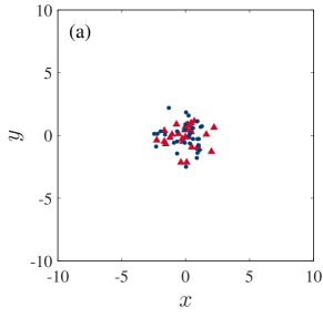
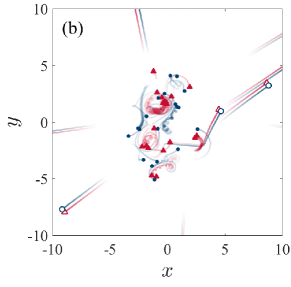
Figure 1: Point-vortex simulation (with a low number of vortices for clarity). Snapshots of vortex configurations at $t=0$ (a) and $t=20$ (b). The range of the display ($-10\leq x,y\leq 10$) is for visualization only (the computational domain is the infinite plane). Vortices (anticlockwise rotation) and antivortices (clockwise circulation) are marked with solid red triangles and solid blue circles respectively. Vortices comprising dipoles (vortex-antivortex pairs) are marked with hollow triangles and circles. The fading comet tails visualize vortex trajectories thus helping the identification of vortex dipoles which ‘evaporate’ from the cluster.

The two processes are qualitatively illustrated in Fig. 1 (with reduced number of vortices for clarity). The evaporating dipoles, marked in Fig. 1(b) with hollow symbols, move away from the cluster along straight trajectories (highlighted by the comet tails), whereas vortices in the cluster move along zig-zagging trajectories. The effect is described by the first movie in the Supplementary Material supple1 .

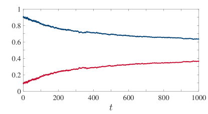
Figure 2: Point-vortex simulation. Fraction $N_{0}(t)/N$ of vortices that remain in the cluster (top blue curve), and fraction $N_{1}(t)/N$ of vortices that form dipoles (bottom red curve), plotted vs. time $t$ and averaged over 10 realizations.

To distinguish the evaporation processes from the spatial diffusion of the main cluster it is useful to divide the vortices in two groups: the vortex dipoles and the main cluster. This distinction requires a consistent definition of what a vortex dipole is. We deem two vortices of opposite circulation to form a dipole if they satisfy the following criteria: (i) the separation $\delta$ between the vortices is less than the separation between either vortex and any other vortex; they are mutually closest to each other, (ii) $\delta$ is less than half the separation between either vortex and the nearest vortex of the same circulation. By numerically experimenting, we find that relaxing or restricting the threshold value for the second criteria by a factor of two has negligible effect on the identification of dipoles. At each time during the evolution we count the numbers $N_{0}(t)$ of vortices which are part of the cluster and the number $N_{1}(t)$ of vortices which are evaporating dipoles. Since in the point vortex model vortices cannot annihilate, the total number of vortices, $N=N_{0}(t)+N_{1}(t)$, remains constant. Figure 2 shows the relative fractions $N_{0}/N$ and $N_{1}/N$ as a function of time. Notice that approximately $20\%$ of the vortices are identified as vortex dipoles already at $t=0$, and that the rate at which vortex dipoles form decreases with time, with approximately 1/3 of vortices having become dipoles when the simulation is stopped.

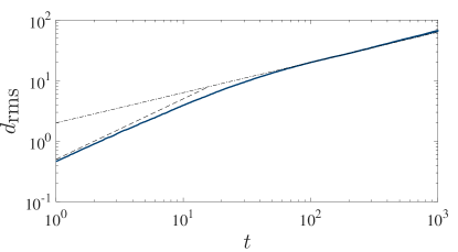
Figure 3: Point-vortex simulation. Root mean square deviation of vortices from their initial position, $d_{\text{rms}}$, vs. time, $t$. Only the vortices which are identified as part of the cluster are used in the calculation of $d_{\text{rms}}$. The dashed and dot-dashed lines correspond to $t$ and $t^{1/2}$ scalings respectively.

By restricting our attention to the $N_{0}(t)$ vortices which remain in the cluster, we calculate the root mean square deviation of vortices from their initial positions, $d_{rms}$, averaging over 10 realizations. Figure 3 shows that the initial linear spread, $d_{\text{rms}}\sim t$, is followed by $d_{\text{rms}}\sim t^{1/2}$ at large $t$, the typical scaling of diffusion processes Uhlenbeck1930 . Similarly to Brownian motion, in which particles follow linear trajectories before colliding with other particles, initially vortices move away at constant speed from their starting positions, leading to the linear (ballistic) spread, until the direction of their motion is altered by approaching another vortex close enough for its contribution to the velocity field to become dominant; a succession of such events appears to behave as a random walk. This interpretation is supported by the observation that the change in behaviour from $d_{\text{rms}}\sim t$ to $d_{\text{rms}}\sim t^{1/2}$ occurs when $d_{\text{rms}}\sim\sigma_{0}$.

III.2 Point vortices in a disc

To make the point vortex model more realistic and include the presence of the condensate’s boundary, we perform numerical simulations within a circular disc of radius $a$ using Eq. (6), rather than Eq. (3). The scenario which we have described (evaporating dipoles and slowly diffusing cluster) does not change, but a new feature arises: when a vortex dipole approaches the disc’s boundary, the distance $\delta$ between the vortex and the antivortex increases to conserve energy, until, close to the boundary, the vortex pair breaks up. The vortex and the antivortex, now separated, travel in opposite directions along the circular boundary, driven by their images. Consider for example the fate of the vortex: as it travels along the boundary, eventually it will meet an antivortex (travelling along the boundary in opposite direction) resulting from the break-up of a different vortex dipole, which has reached the boundary too; when the distance $\delta$ between vortex and antivortex becomes less than the distance to the boundary, the vortex and the antivortex make a sharp turn together, forming a new vortex dipole which travels radially towards the centre of the disc. A similar fate is met by the antivortex. In other words, the boundary effectively re-injects evaporating vortex dipoles back against the main cluster. This effect complicates the interpretation of the results. Clearly the effect is absent if the radius of the disc, $a$, is much larger than the size of the initial vortex cluster, $\sigma_{0}$, and we limit our analysis to times shorter than the time taken by evaporating vortex dipoles to reach the boundary. However there are experimental limitations on the size of a 2D condensate, and the question remains as to whether the reflection of vortex dipoles by the boundary revealed by the point vortex model is physically realistic, and whether it prevents clear separation between evaporating dipoles and main cluster in an actual experiment; we shall have to return to this effect when discussing the GPE model.

III.3 The GPE model

We now turn the attention to the GPE model in which the condensate is confined within a box trap. Here we present only results obtained using circular box traps, but we have repeated the simulations in square box traps and find the same qualitative behaviour, indicating that our results are robust to the trap geometry.

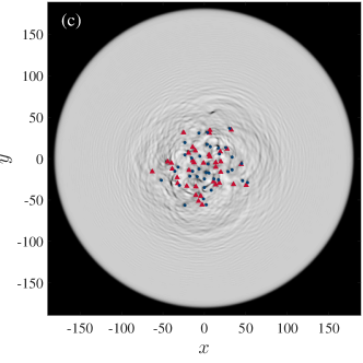
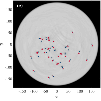
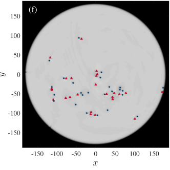
Figure 4: GPE simulation (circular box trap). Plots of the condensate’s density $|\psi|^{2}$ on the $x,y$ plane at $t=0$ (a), $t=30$ (b), $t=60$ (c), $t=90$ (d), $t=500$ (e) and $t=1000$ (f). Positive and negative vortices are marked by solid red triangles and solid blue circles respectively. Note the sound waves generated by vortices, particularly in panels (b), (c) and (d).

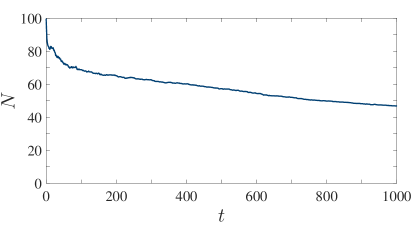
Figure 5: GPE simulations (circular box trap). Number of vortices $N$ at time $t$ averaged over $20$ simulations.

The typical evolution of the initial vortex configuration is shown in Fig. 4, where we plot the density of the condensate at successive selected times. The dark spots in the figure are the density-depleted vortex cores, which we label with red triangles and blue circles (as in Fig. 1 to distinguish positive from negative vortices). As for the point vortices, we observe that fast vortex dipoles evaporate from the slower spreading vortex cluster. Unlike point vortices, however, vortices in the GPE model excite density waves when they accelerate Leadbeater2003 ; Parker2005 . These waves are the ripples clearly visible in Fig. 4, particularly at early stages when vortices are closer to each other and undergo more rapid velocity changes. Moreover, unlike the point vortex model, the total number of vortices is not constant, as shown in Fig. 5, because some vortices collide and annihilate during the real time evolution, particularly again at early stages, when vortices are closer to each other.

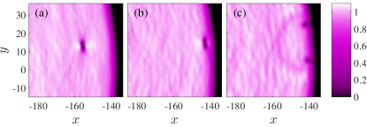
Figure 6: GPE simulation in a circular box trap. Density snapshots are at (a) $t/\tau=250$, (b) $t/\tau=275$, (c) $t/\tau=300$, with $x$ and $y$ in units of $\xi$. A vortex dipole is seen approaching the boundary in (a), meeting the boundary in (b), separating into constituent vortex and antivortex which travel along the boundary in (c), emitting sound waves in this interaction. The colour scale is not linear but chosen to highlight small density perturbations. A movie supple2 shows this interaction in full.

Figure 6 shows that vortices which reach the boundary of the condensate are re-injected back, exactly as found by the point vortex model in Section III.2. Figure 6 illustrates the effect in a box trap with $\alpha=100$ and $R_{0}=200$; similar results are found with less steep confinement, e.g. $\alpha=15$. We think that this re-injection takes place only at the lowest temperatures described by the GPE. Finite-temperature effects cause friction between the vortices and the cloud of thermal atoms. For example, an isolated vortex spirals out of the condensate Jackson2009 and a vortex dipole shrinks and vanishes, generating a Jones-Roberts soliton. We know that thermal atoms are concentrated near the trap’s boundary where the condensate’s density vanishes Proukakis2008 ; Jackson2009 . Therefore, even at relatively low temperature, we expect that vortices will suffer friction in the vicinity of the boundary. This friction can be modelled by replacing $i\partial/\partial t$ at the left-hand side of Eq. (7) with $(i-\gamma)\partial/\partial t$ where $\gamma$ is a small phenomenological parameter which we make radius-dependent by setting

$\displaystyle\gamma(r)=\begin{cases}0,&\text{if $0\leq r<150$}.\\ \dfrac{\gamma_{c}}{2}\left[1+\tanh\left\{\pi(r^{\prime}-1)\right\}\right],&\text{if $150\leq r<160$},\\ \gamma_{c},&\text{otherwise},\end{cases}$

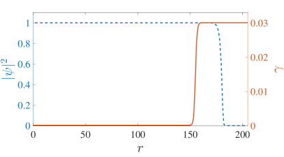
Figure 7: GPE simulation in a circular box trap with localized damping. Density $|\psi|^{2}$ (dashed blue line) and phenomenological damping $\gamma$ (solid red line) are plotted against radius. Note the separate $y$-axis scales for each line.

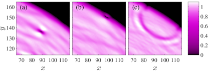
Figure 8: GPE simulation in a circular box trap with localized damping near boundaries. Density snapshots are at (a) $t/\tau=225$, (b) $t/\tau=250$, (c) $t/\tau=275$, with $x$ and $y$ in units of $\xi$. A dipole is seen approaching the boundary in (a), annihilates with the boundary in (b), producing a sound wave which can be seen spreading back into the condensate in (c). A movie supple3 shows this interaction in full.

where $r^{\prime}=(r-150)/\beta$, $\beta=5$ controls the width of the transition from $\gamma=0$ to $\gamma=\gamma_{c}$, and $\gamma_{c}=0.03$ (the value inferred from experiments and commonly used Choi1998 ; Tsubota2001 ), with the tanh function providing a smooth transition between regimes (a step function may reflect vortices and sound waves). The profile of the localized damping is shown with the density profile of the condensate in Fig. 7. With this finite-temperature correction, we find that most vortex dipoles annihilate at the boundary, producing sound waves that spread back into the bulk of the condensate without affecting much the spread of the vortex cluster, as shown in Fig. 8.

III.4 Effective diffusion

Using the point vortex model or the GPE model, we proceed with the analysis as initially described for point vortices. First we separate the fast-moving vortex dipoles from the vortices which remain in the cluster behind which we further analyse. By performing a number of simulations (typically 20 to 40), we obtain the ensemble-averaged root mean square deviation $d_{\text{rms}}(t)$ of the vortices in the cluster from their initial positions as a function of time using Eq. (2). In the case of a scalar field $f(x,y,t)$ which satisfies the 2D diffusion equation

$$\frac{\partial f}{\partial t}=\nu\,\nabla^{2}f,$$ (10)

with constant diffusion coefficient $\nu$, the root mean square deviation $d_{\text{rms}}(t)$ and $\nu$ are related by

$$\nu=\frac{d^{2}_{\text{rms}}(t)}{4t},$$ (11)

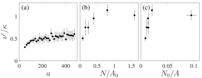
Figure 10: Ratio $\nu^{\prime}/\kappa$ of effective diffusion coefficient and quantum of circulation for (a): point vortex model in a disc, vs. disc radius $a$ for $N/A_{0}=0.08$, (b): point vortex model in infinite domain, vs. initial number density $N/A_{0}$, where $A_{0}=\pi\sigma_{0}^{2}$ where $\sigma_{0}$ is the width of the initial vortex distribution, (c): point vortex model in infinite domain, vs. instanteneous number density $N_{0}/A$, where $N_{0}$ is the number of vortices remaining in the cluster and $A=\pi\sigma_{x}\sigma_{y}$, computed at the point at which $\nu^{\prime}/\kappa$ is computed. In all panels the data represent mean values with $95\%$ confidence intervals indicated by vertical (and in (c) horizontal) black lines.

Using Eq. (11), we define an effective diffusion coefficient $\nu^{\prime}$ representing the spatial spreading of the vortex configuration. In order to combine results obtained via the point vortex model and the GPE model, it is convenient to express $\nu^{\prime}$ in terms of the quantum of circulation $\kappa$. The results are presented in Fig. 9 where we plot $\nu^{\prime}/\kappa$ vs. $t$. We observe that, for large $t$, $\nu^{\prime}/\kappa$ tends to settle down to a constant. For the point vortex model in the infinite domain we find that $\nu^{\prime}/\kappa\approx 1$, a result which is expected from dimensional arguments Tsubota2003 , but still surprising because the fluids which we have considered in our models are inviscid. However, within the circular domain, Fig. 9 shows that $\nu^{\prime}/\kappa\approx 0.5$ with both the point vortex and GPE models, that is to say irrespective of the presence or the absence of density waves and vortex annihilations. We see similar behaviour in the GPE simulations if the domain is square, indicating that the phenomenon is not sensitive to the shape of the confining geometry. The reduced $\nu^{\prime}/\kappa$ appears to be due to confinement itself (that is, the image vortices, which are implicit in the GPE MasonBerloff2008 ): Fig. 10, obtained using the point vortex model, shows that $\nu^{\prime}/\kappa$ increases as the radius $a$ of the disc increases, and that it tends to unity only if the initial vortex density $N/A$ is large enough to provide sufficient scattering events of vortices.

With either the point vortex or the GPE model, each initial condition (a set of random vortices of zero net polarity placed in a prescribed initial region) has different energy $E$ and angular momentum $L_{z}$ which are preserved by the time evolution (with the exception of the GPE model with damping). If we plot $\nu^{\prime}/\kappa$ vs. $E$ or $L_{z}$ from all simulations we observe a cloud of points with no significant dependence of $\nu^{\prime}/\kappa$ vs. $E$ or $L_{z}$. Thus we conclude that our result do not depend on the initial condition, although the spread in values of $E$ and $L_{z}$ may contribute to the error bars of Fig. 9. An experiment to study the diffusion of vortices in a trapped atomic condensate is also likely to start from vortices which are randomly generated, as for our numerical simulations.

IV Discussion

In conclusion, both the point vortex model and the GPE model predict that quantum vortices, if initially localized in a region, spread out in space as a combination of two processes: the formation and fast evaporation of vortex-antivortex pairs (vortex dipoles), and the slower spread of the remaining vortex cluster. The latter, which can be modelled as a diffusion process, is insensitive to the presence of density waves and annihilations, and depends essentially on the Eulerian interaction between vortices which is captured by a model as simple as the point vortex model. This is remarkable: the classical diffusion of vorticity emerges in a fluid without viscosity (a superfluid) from the interaction of many quantum vortices. Quantitatively, the value of the effective diffusion coefficient $\nu^{\prime}$ is in the range $0.3<\nu^{\prime}/\kappa<1$, essentially of the order of the quantum of circulation as predicted by dimensional argument. In confined systems, the diffusion coefficient is reduced by the effect of image vortices.

Both the evaporation of vortex dipoles and the spread of the vortex cluster should be visible in trapped atomic Bose-Einstein condensates at sufficiently low temperatures. The presence of the thermal cloud near the edge of the condensate prevents evaporating dipoles from being re-injected into the vortex cluster and thus promotes a cleaner realization of vortex diffusion than at strictly zero temperature.

Our values of $\nu^{\prime}/\kappa$ are slightly larger but in fair agreement with $\nu^{\prime}/\kappa\approx 0.1$ reported by Tsubota et al Tsubota2003 , and in the related (but not the same as spatial spreading) problem of the decay of superfluid turbulence Walmsley2014 ; Zmeev2015 ; Babuin2016 . The difference is probably due to the fact that our calculation is two-dimensional and lacks three-dimensional effects such as vortex reconnections and Kelvin waves. Further work will explore the problem in three dimensions using the GPE as well as the vortex filament model.

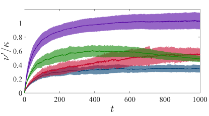
Figure 9: Ratio $\nu^{\prime}/\kappa$ of effective diffusion coefficient and quantum of circulation for (top to bottom) point vortex model in infinite domain (purple curve), point vortex model in circular disc (green curve), GPE simulations in the circular box trap with damping near boundaries (blue curve), and in a square box trap (red curve). The $95\%$ confidence intervals are indicated by the shaded regions.

- (1) C. F. Barenghi and N. G. Parker, A Primer on Quantum Fluids (Springer, Berlin, 2016).
- (2) E. Hodby, G. Hechenblaikner, S. A. Hopkins, M. O. Marago, and C. J. Foot, Phys. Rev. Lett. 88, 010405 (2001).
- (3) J. R. Abo-Shaeer, C. Raman, J. M. Vogels, and W. Ketterle, Science 292, 476 (2001).
- (4) E. A. L. Henn et al., Phys. Rev. A 79, 043618 (2009).
- (5) T. W. Neely, A. S. Bradley, E. C. Samson, S. J. Rooney, E. M. Wright, K. J. H. Law, R. Carretero-Gonzáles, P. G. Kevrekidis, M. J. Davis, and B. P. Anderson, Phys. Rev. Lett. 111, 235301 (2013).
- (6) W. J. Kwon, G. Moon, J. Y. Choi, S. W. Seo, and Y. I. Shin, Phys. Rev. A 90, 063627 (2014).
- (7) M.T. Reeves, B. P. Anderson, and A. S. Bradley, Phys. Rev. A 86, 053621 (2012).
- (8) C. F. Barenghi, N. G. Parker, N. P. Proukakis, and C. S. Adams, J. Low Temp. Phys. 138, 629 (2005).
- (9) M. Karl and T. Gasenzer, New Journal of Physics 19, 093014 (2017).
- (10) G. W. Stagg, A. J. Allen, N. G. Parker, and C. F. Barenghi, Phys. Rev. A 91, 013612 (2015).
- (11) A. Cidrim, F. E. A. dos Santos, L. Galantucci, V. S. Bagnato, and C. F. Barenghi, Phys. Rev. A 93, 033651 (2016).
- (12) A. J. Groszek, T. P. Simula, D. M. Paganin, and K. Helmerson, Phys. Rev. A 93, 043614 (2016).
- (13) A. W. Baggaley and C. F.. Barenghi, Decay of two dimensional quantum turbulence, Phys. Rev. A 97, 033601 (2018).
- (14) A. C. White, C. F. Barenghi, and N. P. Proukakis, Phys. Rev. A 86, 013635 (2012).
- (15) T. Simula, M. J. Davis and K. Helmerson, Kristian, Phys. Rev. Lett. 113, 165302 (2014).
- (16) T. P. Billam, M. T. Reeves, B. P. Anderson, and A. S. Bradley, Phys. Rev. Lett. 112, 145301 (2014).
- (17) G. Gauthier, M. T. Reeves, X. Yu, A. S. Bradley, M. Baker, T. A. Bell, H. Rubinsztein-Dunlop, M. J. Davis and T. W. Neely, arXiv:1801.06951 (2018).
- (18) S. P. Johnstone, A. J. Groszek, P. T. Starkey, C. J. Billington, T. P. Simula and K. Helmerson, arXiv:1801.06952 (2018).
- (19) R. H. Kraichnan and D. Montgomery, Rep. Prog. Phys. 43, (1980).
- (20) J. A. Viecelli, Phys. Fluids 7, 6 (1995).
- (21) C. N. Weiler, T. W. Neely, D. R. Scherer, A. S. Bradley, M. J. Davis, and B. P. Anderson, Nature 455, 948 (2008).
- (22) G. Lamporesi, S. Donadello, S. Serafini, F. Dalfovo, and G. Ferrari, Nat. Phys. 9, 656 (2013).
- (23) L. Chomaz, L. Corman, T. Bienaime, R. Desbuquois, C. Weitenberg, S. Nascimbene, J. Beugnon, and J. Dalibard, Nat. Commun. 6, 6162 (2015).
- (24) S. Donadello, S. Serafini, T. Bienaime, F. Dalfovo, G. Lamporesi, and G. Ferrari, Phys. Rev. A 94, 023628 (2016).
- (25) J. Beugnon, and N. Navon, J. Phys. B 50, 022002 (2017).
- (26) S. Serafini, L. Galantucci, E. Iseni, T. Bienaime, R. N. Bisset, C. F. Barenghi, F. Dalfovo, G. Lamporesi and G. Ferrari, Phys. Rev. X 7, 021031 (2017)
- (27) T. W. Neely, E. C. Samson, A. S. Bradley, M. J. Davis, and B. P. Anderson, Phys. Rev. Lett. 104, 160401 (2010).
- (28) W. J. Kwon, S. W. Seo, and Y. Shin Phys. Rev. A 92, 033613, (2015).
- (29) A.W. Baggaley and N. G. Parker, arXiv:1803.00277, (2018).
- (30) T. Kanai, W. Guo and M. Tsubota, arXiv:1803.03747, (2018).
- (31) K. Sasaki, N. Suzuki and H. Saito, Phys. Rev. Lett. 104, 150404 (2010).
- (32) G. W. Stagg, N. G. Parker and C. F. Barenghi, J. Phys. B 47, 095304 (2014).
- (33) W. J. Kwon, J. H. Kim, S. W. Seo, and Y. I. Shin, Phys. Rev. Lett. 117, 245301 (2016).
- (34) P. G. Saffman Vortex Dynamics, Cambridge University Press (1992).
- (35) S. Middelkamp, P. J. Torres, P. G. Kevrekidis, D. J. Frantzeskakis, R. Carretero-Gonzalez, P. Schmelcher, D. V. Freilich, and D. S. Hall, Phys. Rev. A 84, 011605(R) (2011).
- (36) D. V. Freilich, D. M. Bianchi, A. M. Kaufman, T. K. Langin, and D. S. Hall, Science 329, 1182 (2010).
- (37) A. J. Allen, E. Zaremba, C. F. Barenghi, and N. P. Proukakis, Phys. Rev. A 87, 013630 (2013).
- (38) H. Aref, J. Math. Phy. 48, 065401 (2007).
- (39) P. K. Newton, The N-vortex problem, Springer (2001) .
- (40) T. P. Meyrath, F. Schreck, J. L. Hanssen, C. S. Chuu and M. G. Raizen, Phys. Rev. A 71, 041604(R) (2005).
- (41) J. J. P. van Es, P. Wicke, A. H. van Amerongen, C. Retif, S. Whitlock, and N. J. van Druten, J. Phys. B 43, 155002 (2010).
- (42) A. L. Gaunt, T. F. Schmidutz, I. Gotlibovych, R. P. Smith, and Z. Hadzibabic, Phys. Rev. Lett. 110, 200406 (2013).
- (43) L. Chomaz, L. Corman, T. Bienaime, R. Desbuquois, C. Weitenberg, S. Nascimbene, J. Beugnon, and J. Dalibard, Nat. Commun. 6, 6162 (2015).
- (44) P. Bader, S. Blanes, and F. Casas, J. Chem. Phys. 138, 124117 (2013).
- (45) M. Caliari and S. Zuccher, Comput. Phys. Commun. 222, 46 (2018).
- (46) See Supplemental Material at [URL when accepted] for animation performed using the point vortex model.
- (47) C. F. Barenghi and D. C. Samuels, Phys. Rev. Lett. 89, 155302 (2002).
- (48) G. E. Uhlenbeck and L. S. Ornstein, Phys. Rev. 36, 5 (1930).
- (49) M. Leadbeater, D.C. Samuels, C.F. Barenghi, and C.S. Adams, Phys. Rev. A 67, 015601 (2003).
- (50) B. Jackson, N. P. Proukakis, C. F. Barneghi, and E. Zaremba, Phys. Rev. A 79, 053615 (2009).
- (51) N.P. Proukakis and B. Jackson, J. Phys. B: At. Mol. Opt. Phys. 41 203002 (2008).
- (52) S. Choi, S. A. Morgan, and K. Burnett, Phys. Rev. A 57, 4057 (1998).
- (53) M. Tsubota, K. Kasamatsu, and M. Ueda, Phys. Rev. A 65, 023603 (2001).
- (54) M. Tsubota, T. Araki, and W.F. Vinen, Physica B 224, 329 (2003).
- (55) P. Mason and N. G. Berloff, Phys. Rev. A 77, 032107 (2008).
- (56) P. Walmsley, D. Zmeev, F. Pakpour, and A. Golov, Proc. Nat. Acad. Sci. (USA) 111 suppl. 1, 4691 (2014).
- (57) D. E. Zmeev, P. M. Walmsley, A. I. Golov, P. V. E. McClintock, S. N. Fisher, and W. F. Vinen, Phys. Rev. Lett. 115, 155303 (2015).
- (58) S. Babuin, E. Varga. L. Skrbek, E. Leveque, and P-E. Roche, Europhys. Lett. 106, 24006 (2014).
- (59) See Supplemental Material at [URL when accepted] for an animation of the the interaction between a vortex dipole and the boundary performed using the GPE model without damping.
- (60) See Supplemental Material at [URL when accepted] for an animation of the the interaction between a vortex dipole and the boundary performed using the GPE model with damping.