Alternating Randomized Block Coordinate Descent

Abstract

Block-coordinate descent algorithms and alternating minimization methods are fundamental optimization algorithms and an important primitive in large-scale optimization and machine learning. While various block-coordinate-descent-type methods have been studied extensively, only alternating minimization – which applies to the setting of only two blocks – is known to have convergence time that scales independently of the least smooth block. A natural question is then: is the setting of two blocks special?

We show that the answer is “no” as long as the least smooth block can be optimized exactly – an assumption that is also needed in the setting of alternating minimization. We do so by introducing a novel algorithm AR-BCD, whose convergence time scales independently of the least smooth (possibly non-smooth) block. The basic algorithm generalizes both alternating minimization and randomized block coordinate (gradient) descent, and we also provide its accelerated version – AAR-BCD. As a special case of AAR-BCD, we obtain the first nontrivial accelerated alternating minimization algorithm.

1 Introduction

First-order methods for minimizing smooth convex functions are a cornerstone of large-scale optimization and machine learning. Given the size and heterogeneity of the data in these applications, there is a particular interest in designing iterative methods that, at each iteration, only optimize over a subset of the decision variables (Wright, 2015).

This paper focuses on two classes of methods that constitute important instantiations of this idea. The first class is that of block-coordinate descent methods, i.e., methods that partition the set of variables into $n\geq 2$ blocks and perform a gradient descent step on a single block at every iteration, while leaving the remaining variable blocks fixed. A paradigmatic example of this approach is the randomized Kaczmarz algorithm of (Strohmer & Vershynin, 2009) for linear systems and its generalization (Nesterov, 2012). The second class is that of alternating minimization methods, i.e., algorithms that partition the variable set into only $n=2$ blocks and alternate between exactly optimizing one block or the other at each iteration (see, e.g., (Beck, 2015) and references therein).

Besides the computational advantage in only having to update a subset of variables at each iteration, methods in these two classes are also able to exploit better the structure of the problem, which, for instance, may be computationally expensive only in a small number of variables. To formalize this statement, assume that the set of variables is partitioned into $n\leq N$ mutually disjoint blocks, where the $i^{\mathrm{th}}$ block of variable $\mathbf{x}$ is denoted by $\mathbf{x}^{i}$, and the gradient corresponding to the $i^{\mathrm{th}}$ block is denoted by $\nabla_{i}f(\mathbf{x})$. Each block $i$ will be associated with a smoothness parameter $L_{i},$ I.e., $\forall\mathbf{x},\mathbf{y}\in\mathbb{R}^{N}$:

$$\|\nabla_{i}f(\mathbf{x}+I_{N}^{i}\mathbf{y})-\nabla_{i}f(\mathbf{x})\|_{*}\leq L_{i}\|\mathbf{y}^{i}\|,$$ (1.1)

where $I_{N}^{i}$ is a diagonal matrix whose diagonal entries equal one for coordinates from block $i$, and are zero otherwise.

In this setting, the convergence time of standard randomized block-coordinate descent methods, such as those in (Nesterov, 2012), scales as $O\left(\frac{\sum_{i}L_{i}}{\epsilon}\right)$, where $\epsilon$ is the desired additive error. By contrast, when $n=2,$ the convergence time of the alternating minimization method (Beck, 2015) scales as $O\left(\frac{L_{\min}}{\epsilon}\right),$ where $L_{\min}$ is the minimum smoothness parameter of the two blocks. This means that one of the two blocks can have arbitrarily poor smoothness (including $\infty$), as long it is easy to optimize over it. Some important examples with a nonsmooth block (with smoothness parameter equal to infinity) can be found in (Beck, 2015). Additional examples of problems for which exact optimization over the least smooth block can be performed efficiently are provided in Appendix B.

In this paper, we address the following open question, which was implicitly raised by (Beck & Tetruashvili, 2013): can we design algorithms that combine the features of randomized block-coordinate descent and alternating minimization? In particular, assuming we can perform exact optimization on block $n$, can we construct a block-coordinate descent algorithm whose running time scales with $O(\sum_{i=1}^{n-1}L_{i}),$ i.e., independently of the smoothness $L_{n}$ of the $n^{\mathrm{th}}$ block? This would generalize both existing block-coordinate descent methods, by allowing one block to be optimized exactly, and existing alternating minimization methods, by allowing $n$ to be larger than $2$ and requiring exact optimization only on a single block.

We answer these questions in the affirmative by presenting a novel algorithm: alternating randomized block coordinate descent (AR-BCD). The algorithm alternates between an exact optimization over a fixed, possibly non-smooth block, and a gradient descent or exact optimization over a randomly selected block among the remaining blocks. For two blocks, the method reduces to the standard alternating minimization, while when the non-smooth block is empty (not optimized over), we get randomized block coordinate descent (RCDM) from (Nesterov, 2012).

Our second contribution is AAR-BCD, an accelerated version of AR-BCD, which achieves the accelerated rate of $\frac{1}{k^{2}}$ without incurring any dependence on the smoothness of block $n$. Furthermore, when the non-smooth block is empty, AAR-BCD recovers the fastest known convergence bounds for block-coordinate descent (Qu & Richtárik, 2016; Allen-Zhu et al., 2016; Nesterov, 2012; Lin et al., 2014; Nesterov & Stich, 2017). As a special case, AAR-BCD provides the first accelerated alternating minimization algorithm, obtained directly from AAR-BCD when the number of blocks equals two. Another conceptual contribution is our extension of the approximate duality gap technique of (Diakonikolas & Orecchia, 2017), which leads to a general and more streamlined analysis.

Finally, to illustrate the results, we perform a preliminary experimental evaluation of our methods against existing block-coordinate algorithms and discuss how their performance depends on the smoothness and size of the blocks.

Related Work

Alternating minimization and cyclic block coordinate descent are old and fundamental algorithms (Ortega & Rheinboldt, 1970) whose convergence (to a stationary point) has been studied even in the non-convex setting, in which they were shown to converge asymptotically under the additional assumptions that the blocks are optimized exactly and their minimizers are unique (Bertsekas, 1999). However, even in the non-smooth convex case, methods that perform exact minimization over a fixed set of blocks may converge arbitrarily slowly. This has lead scholars to focus on the case of smooth convex minimization, for which nonasymptotic convergence rates were obtained recently in (Beck & Tetruashvili, 2013; Beck, 2015; Sun & Hong, 2015; Saha & Tewari, 2013). However, prior to our work, convergence bounds that are independent of the largest smoothness parameter were only known for the setting of two blocks.

Randomized coordinate descent methods, in which steps over coordinate blocks are taken in a non-cyclic randomized order (i.e., in each iteration one block is sampled with replacement) were originally analyzed in (Nesterov, 2012). The same paper (Nesterov, 2012) also provided an accelerated version of these methods. The results of (Nesterov, 2012) were subsequently improved and generalized to various other settings (such as, e.g., composite minimization) in (Lee & Sidford, 2013; Allen-Zhu et al., 2016; Nesterov & Stich, 2017; Richtárik & Takáč, 2014; Fercoq & Richtárik, 2015; Lin et al., 2014). The analysis of the different block coordinate descent methods under various sampling probabilities (that, unlike in our setting, are non-zero over all the blocks) was unified in (Qu & Richtárik, 2016) and extended to a more general class of steps within each block in (Gower & Richtárik, 2015; Qu et al., 2016).

Our results should be carefully compared to a number of proximal block-coordinate methods that rely on different assumptions (Tseng & Yun, 2009; Richtárik & Takáč, 2014; Lin et al., 2014; Fercoq & Richtárik, 2015). In this setting, the function $f$ is assumed to have the structure $f_{0}(\mathbf{x})+\Psi(\mathbf{x}),$ where $f_{0}$ is smooth, the non-smooth convex function $\Psi$ is separable over the blocks, i.e., $\Psi(\mathbf{x})=\sum_{i=1}^{n}\Psi_{i}(\mathbf{x}_{i})$, and we can efficiently compute the proximal operator of each $\Psi_{i}$. This strong assumption allows these methods to make use of the standard proximal optimization framework. By contrast, in our paper, the convex objective can be taken to have an arbitrary form, where the non-smoothness of a block need not be separable, though the function is assumed to be differentiable.

2 Preliminaries

We assume that we are given oracle access to the gradients of a continuously differentiable convex function $f:\mathbb{R}^{N}\rightarrow\mathbb{R}$, where computing gradients over only a subset of coordinates is computationally much cheaper than computing the full gradient. We are interested in minimizing $f(\cdot)$ over $\mathbb{R}^{N}$, and we denote $\mathbf{x}_{*}=\operatorname*{argmin}_{\mathbf{x}\in\mathbb{R}^{N}}f(\mathbf{x})$. We let $\|\cdot\|$ denote an arbitrary (but fixed) norm, and $\|\cdot\|_{*}$ denote its dual norm, defined in the standard way: $\|\mathbf{z}\|_{*}=\sup_{\mathbf{x}\in\mathbb{R}^{N}:\|\mathbf{x}\|=1}\left\langle\mathbf{z},\mathbf{x}\right\rangle$.

Let $I_{N}$ be the identity matrix of size $N$, $I_{N}^{i}$ be a diagonal matrix whose diagonal elements $j$ are equal to one if variable $j$ is in the $i^{\mathrm{th}}$ block, and zero otherwise. Notice that $I_{N}=\mathop{\textstyle\sum}_{i=1}^{n}I_{N}^{i}$. Let $S_{i}(\mathbf{x})=\{\mathbf{y}\in\mathbb{R}^{N}:(I_{N}-I_{N}^{i})\mathbf{y}=(I_{N}-I_{N}^{i})\mathbf{x}\}$, that is, $S_{i}$ contains all the points from $\mathbb{R}^{N}$ whose coordinates differ from those of $\mathbf{x}$ only over block $i$.

We denote the smoothness parameter of block $i$ by $L_{i}$, as defined in Equation (1.1). Equivalently, $\forall\mathbf{x},\mathbf{y}\in\mathbb{R}^{N}$:

$$f(\mathbf{x}+I_{N}^{i}\mathbf{y})\leq f(\mathbf{x})+\left\langle\nabla_{i}f(\mathbf{x}),\mathbf{y}^{i}\right\rangle+\frac{L_{i}}{2}\|\mathbf{y}^{i}\|^{2}.$$ (2.1)

The gradient step over block $i$ is then defined as:

$$T_{i}(\mathbf{x})$$ (2.2)

$$\hskip 5.69046pt=\operatorname*{argmin}_{\mathbf{y}\in{S}_{i}(\mathbf{x})}\Big{\{}\left\langle\nabla f(\mathbf{x}),\mathbf{y}-\mathbf{x}\right\rangle+\frac{L_{i}}{2}\|\mathbf{y}-\mathbf{x}\|^{2}\Big{\}}.$$

By standard arguments (see, e.g., Exercise 3.27 in (Boyd & Vandenberghe, 2004)):

$$f(T_{i}(\mathbf{x}))-f(\mathbf{x})\leq-\frac{1}{2L_{i}}\|\nabla_{i}f(\mathbf{x})\|_{*}^{2}.$$ (2.3)

Without loss of generality, we will assume that the $n^{\mathrm{th}}$ block has the largest smoothness parameter and is possibly non-smooth (i.e., it can be $L_{n}=\infty$). The standing assumption is that exact minimization over the $n^{\mathrm{th}}$ block is “easy”, meaning that it is computationally inexpensive and possibly solvable in closed form; for some important examples that have this property, see Appendix B. Observe that when block $n$ contains a small number of variables, it is often computationally inexpensive to use second-order optimization methods, such as, e.g., interior point method.

We assume that $f(\cdot)$ is strongly convex with parameter $\mu\geq 0$, where it could be $\mu=0$ (in which case $f(\cdot)$ is not strongly convex). Namely, $\forall\mathbf{x},\mathbf{y}$:

$$f(\mathbf{y})\geq f(\mathbf{x})+\left\langle\nabla f(\mathbf{x}),\mathbf{y}-\mathbf{x}\right\rangle+\frac{\mu}{2}\|\mathbf{y}-\mathbf{x}\|^{2}.$$ (2.4)

When $\mu>0$, we take $\|\cdot\|=\|\cdot\|_{2}$, which is customary for smooth and strongly convex minimization (Bubeck, 2014).

Throughout the paper, whenever we take unconditional expectation, it is with respect to all randomness in the algorithm.

2.1 Alternating Minimization

In (standard) alternating minimization (AM), there are only two blocks of coordinates, i.e., $n=2$. The algorithm is defined as follows. $$\begin{gathered}\mathbf{\hat{x}}_{k}=\operatorname*{argmin}_{\mathbf{x}\in S_{1}(\mathbf{x}_{k-1})}f(\mathbf{x}),\\ \mathbf{x}_{k}=\operatorname*{argmin}_{\mathbf{x}\in S_{2}(\mathbf{\hat{x}}_{k})}f(\mathbf{x}),\\ \mathbf{x}_{1}\in\mathbb{R}^{N}\text{ is an arbitrary initial point.}\end{gathered}$$ (AM) We note that for the standard analysis of alternating minimization (Beck, 2015), the exact minimization step over the smoother block can be replaced by a gradient step (Equation (2.2)), while still leading to convergence that is only dependent on the smaller smoothness parameter.

2.2 Randomized Block Coordinate (Gradient) Descent

The simplest version of randomized block coordinate (gradient) descent (RCDM) can be stated as (Nesterov, 2012):

$$\begin{gathered}\text{Select }i_{k}\in\{1,\dots,n\}\text{ w.p. }p_{i_{k}}>0,\\ \mathbf{x}_{k}=T_{i_{k}}(\mathbf{x}_{k-1}),\\ \mathbf{x}_{1}\in\mathbb{R}^{N}\text{ is an arbitrary initial point,}\end{gathered}$$ (RCDM) where $\sum_{i=1}^{n}p_{i}=1$. A standard choice of the probability distribution is $p_{i}\sim L_{i}$, leading to the convergence rate that depends on the sum of block smoothness parameters.

3 AR-BCD

The basic version of alternating randomized block coordinate descent (AR-BCD) is a direct generalization of (AM) and (RCDM): when $n=2$, it is equivalent to (AM), while when the size of the $n^{\mathrm{th}}$ block is zero, it reduces to (RCDM). The method is stated as follows: $$\begin{gathered}\text{Select }i_{k}\in\{1,\dots,n-1\}\text{ w.p. }p_{i_{k}}>0,\\ \mathbf{\hat{x}}_{k}=T_{i_{k}}(\mathbf{x}_{k-1}),\\ \mathbf{x}_{k}=\operatorname*{argmin}_{\mathbf{x}\in S_{n}(\mathbf{\hat{x}}_{k})}f(\mathbf{x}),\\ \mathbf{x}_{1}\in\mathbb{R}^{N}\text{ is an arbitrary initial point,}\end{gathered}$$ (AR-BCD) where $\sum_{i=1}^{n-1}p_{i}=1$. We note that nothing will change in the analysis if the step $\mathbf{\hat{x}}_{k}=T_{i_{k}}(\mathbf{x}_{k-1})$ is replaced by $\mathbf{\hat{x}}_{k}=\operatorname*{argmin}_{\mathbf{x}\in S_{i_{k}}(\mathbf{x}_{k-1})}f(\mathbf{x})$, since $\min_{\mathbf{x}\in S_{i_{k}}(\mathbf{x}_{k-1})}f(\mathbf{x})\leq f(T_{i_{k}}(\mathbf{x}_{k-1}))$.

In the rest of the section, we show that (AR-BCD) leads to a convergence bound that interpolates between the convergence bounds of (AM) and (RCDM): it depends on the sum of the smoothness parameters of the first $n-1$ blocks, while the dependence on the remaining problem parameters is the same for all these methods.

3.1 Approximate Duality Gap

To analyze (AR-BCD), we extend the approximate duality gap technique (Diakonikolas & Orecchia, 2017) to the setting of randomized block coordinate descent methods. The approximate duality gap $G_{k}$ is defined as the difference of an upper bound $U_{k}$ and a lower bound $L_{k}$ to the minimum function value $f(\mathbf{x}_{*})$. For (AR-BCD), we choose the upper bound to simply be $U_{k}=f(\mathbf{x}_{k+1})$.

The generic construction of the lower bound is as follows. Let $\mathbf{x}_{1},\mathbf{x}_{2},...,\mathbf{x}_{k}$ be any sequence of points from $\mathbb{R}^{N}$ (in fact we will choose them to be exactly the sequence constructed by (AR-BCD)). Then, by (strong) convexity of $f(\cdot)$, $f(\mathbf{x}_{*})\geq f(\mathbf{x}_{j})+\left\langle\nabla f(\mathbf{x}_{j}),\mathbf{x}_{*}-\mathbf{x}_{j}\right\rangle+\frac{\mu}{2}\|\mathbf{x}_{*}-\mathbf{x}_{j}\|^{2}$, $\forall j\in\{1,\dots,k\}$. In particular, if $a_{j}>0$ is a sequence of (deterministic, independent of $i_{j}$) positive real numbers and $A_{k}=\sum_{j=1}^{k}a_{j}$, then:

$$f(\mathbf{x}_{*})\geq \frac{\mathop{\textstyle\sum}_{j=1}^{k}a_{j}f(\mathbf{x}_{j})+\mathop{\textstyle\sum}_{j=1}^{k}a_{j}\left\langle\nabla f(\mathbf{x}_{j}),\mathbf{x}_{*}-\mathbf{x}_{j}\right\rangle}{A_{k}}$$

$$+\frac{\frac{\mu}{2}\sum_{j=1}^{k}a_{j}\|\mathbf{x}_{*}-\mathbf{x}_{j}\|^{2}}{A_{k}}\stackrel{{\scriptstyle\mathrm{\scriptscriptstyle def}}}{{=}}L_{k}.$$ (3.1)

3.2 Convergence Analysis

The main idea in the analysis is to show that $\mathbb{E}[A_{k}G_{k}-A_{k-1}G_{k-1}]\leq E_{k}$, for some deterministic $E_{k}$. Then, using linearity of expectation, $\mathbb{E}[f(\mathbf{x}_{k+1})]-f(\mathbf{x}_{*})\leq\mathbb{E}[G_{k}]\leq\frac{\mathbb{E}[A_{1}G_{1}]}{A_{k}}+\frac{\sum_{j=2}^{k}E_{j}}{A_{k}}$. The bound in expectation can then be turned into a bound in probability, using well-known concentration bounds. The main observation that allows us not to pay for the non-smooth block is:

Observation 3.1.

For $\mathbf{x}_{k}$’s constructed by (AR-BCD), $\nabla_{n}f(\mathbf{x}_{k})=\mathbf{0}$, $\forall k$, where $\mathbf{0}$ is the vector of all zeros.

This observation is essentially what allows us to sample $i_{k}$ only from the first $n-1$ blocks, and holds due to the step $\mathbf{x}_{k}=\operatorname*{argmin}_{\mathbf{x}\in S_{n}(\mathbf{\hat{x}}_{k})}f(\mathbf{x})$ from (AR-BCD).

Denote $R_{\mathbf{x}_{*}^{i}}=\max_{\mathbf{x}\in\mathbb{R}^{N}}\{\|I_{N}^{i}(\mathbf{x}_{*}-\mathbf{x})\|^{2}:f(\mathbf{x})\leq f(\mathbf{x}_{1})\}$, and let us bound the initial gap $A_{1}G_{1}$.

Proposition 3.2.

$\mathbb{E}[A_{1}G_{1}]\leq E_{1}$, where $E_{1}=a_{1}\mathop{\textstyle\sum}_{i=1}^{n-1}\left(\frac{L_{i}}{2p_{i}}-\frac{\mu}{2}\right)R_{\mathbf{x}_{*}^{i}}$.

Proof.

By linearity of expectation, $\mathbb{E}[A_{1}G_{1}]=\mathbb{E}[A_{1}U_{1}]-\mathbb{E}[A_{1}L_{1}].$ The initial lower bound is deterministic, and, by $\nabla_{n}f(\mathbf{x}_{1})=\mathbf{0}$ and duality of norms, is bounded as:

$$\mathbb{E}[A_{1}L_{1}]\geq a_{1}f(\mathbf{x}_{1})-a_{1}\mathop{\textstyle\sum}_{i=0}^{n-1}\|\nabla_{i}f(\mathbf{x}_{1})\|_{*}\|\mathbf{x}_{*}^{i}-\mathbf{x}_{1}^{i}\|$$

$$+a_{1}\frac{\mu}{2}\|\mathbf{x}_{*}-\mathbf{x}_{1}\|^{2}.$$

Using (2.3), if $i_{2}=i$, then:

$$U_{1}=f(\mathbf{x}_{2})\leq f(\mathbf{\hat{x}}_{2})\leq f(\mathbf{x}_{1})-\frac{1}{2L_{i}}\|\nabla_{i}f(\mathbf{x}_{1})\|_{*}^{2}.$$

Since block $i$ is selected with probability $p_{i}$ and $A_{1}=a_{1}$:

$$\mathbb{E}[A_{1}U_{1}]\leq a_{1}f(\mathbf{x}_{1})-\mathop{\textstyle\sum}_{i=1}^{n-1}\frac{a_{1}p_{i}}{2L_{i}}\|\nabla_{i}f(\mathbf{x}_{i})\|_{*}^{2}.$$

Since the inequality $2ab-a^{2}\leq b^{2}$ holds $\forall a,b$, we have:

$$a_{1}\|\nabla_{i}f(\mathbf{x}_{1})\|_{*}\|\mathbf{x}_{*}^{i}-\mathbf{x}_{1}^{i}\|-\frac{a_{1}p_{i}}{2L_{i}}\|\nabla_{i}f(\mathbf{x}_{i})\|_{*}^{2}$$

$$\hskip 28.45274pt\leq\frac{a_{1}L_{i}}{2p_{i}}\|\mathbf{x}_{*}^{i}-\mathbf{x}_{1}^{i}\|^{2},\;\forall i\in\{1,\dots,n-1\}$$

Hence, when $\mu=0$, $\mathbb{E}[A_{1}G_{1}]\leq\sum_{i=1}^{n-1}\frac{a_{1}L_{i}}{2p_{i}}\|\mathbf{x}_{*}^{i}-\mathbf{x}_{1}^{i}\|^{2}$. When $\mu>0,$ since in that case we are assuming $\|\cdot\|=\|\cdot\|_{2}$ (Section 2), $\|\mathbf{x}_{*}-\mathbf{x}_{1}\|^{2}\geq\sum_{i=1}^{n-1}\|\mathbf{x}_{*}^{i}-\mathbf{x}_{1}^{i}\|^{2}$, leading to $\mathbb{E}[A_{1}G_{1}]\leq a_{1}\sum_{i=1}^{n-1}\left(\frac{L_{i}}{2p_{i}}-\frac{\mu}{2}\right)\|\mathbf{x}_{*}^{i}-\mathbf{x}_{1}^{i}\|^{2}$. ∎

We now show how to bound the error in the decrease of the scaled gap $A_{k}G_{k}$.

Lemma 3.3.

$\mathbb{E}[A_{k}G_{k}-A_{k-1}G_{k-1}]\leq E_{k}$, where $E_{k}=a_{k}\sum_{i=1}^{n-1}\left(\frac{{a_{k}}L_{i}}{2A_{k}p_{i}}-\frac{\mu}{2}\right)R_{\mathbf{x}_{*}^{i}}$.

Proof.

Let $\mathcal{F}_{k}$ denote the natural filtration up to iteration $k$. By linearity of expectation and $A_{k}L_{k}-A_{k-1}L_{k-1}$ being measurable w.r.t. $\mathcal{F}_{k}$,

$$\mathbb{E}[A_{k}G_{k}-A_{k-1}G_{k-1}|\mathcal{F}_{k}]$$

$$\hskip 5.69046pt=\mathbb{E}[A_{k}U_{k}-A_{k-1}U_{k-1}|\mathcal{F}_{k}]-(A_{k}L_{k}-A_{k-1}L_{k-1}).$$

With probability $p_{i}$ and as $f(\mathbf{x}_{k+1})\leq f(\mathbf{\hat{x}}_{k+1})$, the change in the upper bound is:

$$A_{k}U_{k}-A_{k-1}U_{k-1}\leq A_{k}f(\mathbf{\hat{x}}_{k+1})-A_{k-1}f(\mathbf{x}_{k})$$

$$\leq a_{k}f(\mathbf{x}_{k})-\frac{A_{k}}{2L_{i}}\|\nabla_{i}f(\mathbf{x}_{k})\|_{*}^{2},$$

where the second line follows from $\mathbf{\hat{x}}_{k+1}=T_{i_{k}}(\mathbf{x}_{k})$ and Equation (2.3). Hence:

$$\mathbb{E}[A_{k}U_{k}-A_{k-1}U_{k-1}|\mathcal{F}_{k}]$$

$$\hskip 28.45274pt\leq a_{k}f(\mathbf{x}_{k})-A_{k}\mathop{\textstyle\sum}_{i=1}^{n-1}\frac{p_{i}}{2L_{i}}\|\nabla_{i}f(\mathbf{x}_{k})\|_{*}^{2}.$$

On the other hand, using the duality of norms, the change in the lower bound is:

$$A_{k}L_{k}-A_{k-1}L_{k-1}$$

$$\hskip 28.45274pt\geq a_{k}f(\mathbf{x}_{k})-a_{k}\mathop{\textstyle\sum}_{i=1}^{n-1}\|\nabla_{i}f(\mathbf{x}_{k})\|_{*}\|\mathbf{x}_{*}^{i}-\mathbf{x}_{k}^{i}\|$$

$$\hskip 39.83368pt+a_{k}\frac{\mu}{2}\|\mathbf{x}_{*}-\mathbf{x}_{k}\|^{2}$$

$$\hskip 28.45274pt\geq a_{k}f(\mathbf{x}_{k})-a_{k}\mathop{\textstyle\sum}_{i=1}^{n-1}\|\nabla_{i}f(\mathbf{x}_{k})\|_{*}\sqrt{R_{\mathbf{x}_{*}^{i}}}$$

$$\hskip 39.83368pt+a_{k}\frac{\mu}{2}\|\mathbf{x}_{*}-\mathbf{x}_{k}\|^{2}.$$

By the same argument as in the proof of Proposition 3.2, it follows that: $\mathbb{E}[A_{k}G_{k}-A_{k-1}G_{k-1}|\mathcal{F}_{k}]\leq a_{k}\sum_{i=1}^{n-1}\left(\frac{L_{i}{a_{k}}}{2A_{k}p_{i}}-\frac{\mu}{2}\right)R_{\mathbf{x}_{*}^{i}}=E_{k}$. Taking expectations on both sides, as $E_{k}$ is deterministic, the proof follows. ∎

We are now ready to prove the convergence bound for (AR-BCD), as follows.

Theorem 3.4.

Let $\mathbf{x}_{k}$ evolve according to (AR-BCD). Then, $\forall k\geq 1$:

1. If $\mu=0:$ $\mathbb{E}[f(\mathbf{x}_{k+1})]-f(\mathbf{x}_{*})\leq\frac{2\mathop{\textstyle\sum}_{i=1}^{n-1}\frac{L_{i}}{p_{i}}R_{\mathbf{x}_{*}^{i}}}{k+3}.$ In particular, for $p_{i}=\frac{L_{i}}{\sum_{i^{\prime}=1}^{n-1}L_{i^{\prime}}},$ $1\leq i\leq n-1$:

   $$\mathbb{E}[f(\mathbf{x}_{k+1})]-f(\mathbf{x}_{*})\leq\frac{2(\sum_{i^{\prime}=1}^{n-1}L_{i^{\prime}})\mathop{\textstyle\sum}_{i=1}^{n-1}R_{\mathbf{x}_{*}^{i}}}{k+3}.$$

   Similarly, for $p_{i}=\frac{1}{n-1}$, $1\leq i\leq n-1:$

   $$\mathbb{E}[f(\mathbf{x}_{k+1})]-f(\mathbf{x}_{*})\leq\frac{2(n-1)\mathop{\textstyle\sum}_{i=1}^{n-1}{L_{i}}R_{\mathbf{x}_{*}^{i}}}{k+3}$$

2. If $\mu>0$, $p_{i}=\frac{L_{i}}{\sum_{i^{\prime}=1}^{n-1}L_{i^{\prime}}}$ and $\|\cdot\|=\|\cdot\|_{2}:$

   $$\mathbb{E}[f(\mathbf{x}_{k+1})]-f(\mathbf{x}_{*})$$

   $$\hskip 28.45274pt\leq\Big{(}1-\frac{\mu}{\sum_{i^{\prime}=1}^{n-1}L_{i^{\prime}}}\Big{)}^{k}$$

   $$\hskip 42.67912pt\cdot\frac{(\sum_{i^{\prime}=1}^{n-1}L_{i^{\prime}})\|(I_{N}-I_{N}^{n})(\mathbf{x}_{*}-\mathbf{x}_{1})\|^{2}}{2}.$$

Proof.

From Proposition 3.2 and Lemma 3.3, by linearity of expectation and the definition of $G_{k}$:

$$\mathbb{E}[f(\mathbf{x}_{k+1})]-f(\mathbf{x}_{*})\leq\mathbb{E}[G_{k}]\leq\frac{\sum_{j=1}^{k}E_{j}}{A_{k}},$$ (3.2)

where $E_{j}=\frac{{a_{j}}^{2}}{A_{j}}\sum_{i=1}^{n-1}\frac{L_{i}}{2p_{i}}R_{\mathbf{x}_{*}^{i}}$.

Notice that the algorithm does not depend on the sequence $\{a_{j}\}$ and thus we can choose it arbitrarily. Suppose that $\mu=0$. Let $a_{j}=\frac{j+1}{2}$. Then $\frac{{a_{j}}^{2}}{A_{j}}=\frac{(j+1)^{2}}{j(j+3)}\leq 1$, and thus: $\frac{\sum_{j=1}^{k}E_{j}}{A_{k}}\leq\frac{2\mathop{\textstyle\sum}_{i=1}^{n-1}\frac{L_{i}}{p_{i}}R_{\mathbf{x}_{*}^{i}}}{k+3},$which proves the first part of the theorem, up to concrete choices of $p_{i}$’s, which follow by simple computations.

For the second part of the theorem, as $\mu>0$, we are assuming that $\|\cdot\|=\|\cdot\|_{2}$, as discussed in Section 2. From Lemma 3.3, $E_{j}=a_{j}\sum_{i=1}^{n-1}\left(\frac{a_{j}L_{i}}{2A_{j}p_{i}}-\frac{\mu}{2}\right)R_{\mathbf{x}_{*}^{i}}$, $\forall j\geq 2$. As $p_{i}=\frac{L_{i}}{\sum_{i^{\prime}=1}^{n-1}L_{i^{\prime}}}$, if we take $\frac{a_{j}}{A_{j}}=\frac{\mu}{\sum_{i^{\prime}=1}^{n-1}L_{i^{\prime}}}$, it follows that $E_{j}=0$, $\forall j\geq 2$. Let $a_{1}=A_{1}=1$ and $\frac{a_{j}}{A_{j}}=\frac{\mu}{\sum_{i^{\prime}=1}^{n-1}L_{i^{\prime}}}$ for $j\geq 2$. Then: $\mathbb{E}[f(\mathbf{x}_{k+1})]-f(\mathbf{x}_{*})\leq\mathbb{E}[G_{k}]\leq\frac{\mathbb{E}[A_{1}G_{1}]}{A_{k}}.$ As $\frac{A_{1}}{A_{k}}=\frac{A_{1}}{A_{2}}\cdot\frac{A_{2}}{A_{3}}\cdot\dots\cdot\frac{A_{k-1}}{A_{k}}$ and $\frac{A_{j-1}}{A_{j}}=1-\frac{a_{j}}{A_{j}}$: $\mathbb{E}[f(\mathbf{x}_{k+1})]-f(\mathbf{x}_{*})\leq\Big{(}1-\frac{\mu}{\sum_{i^{\prime}=1}^{n-1}L_{i^{\prime}}}\Big{)}^{k-1}\mathbb{E}[G_{1}].$ It remains to observe that, from Proposition 3.2, $\mathbb{E}[G_{1}]\leq\big{(}1-\frac{\mu}{\sum_{i^{\prime}=1}^{n-1}L_{i^{\prime}}}\big{)}\frac{(\sum_{i^{\prime}=1}^{n-1}L_{i^{\prime}})\|(I_{N}-I_{N}^{n})(\mathbf{x}_{*}-\mathbf{x}_{1})\|^{2}}{2}$. ∎

We note that when $n=2$, the asymptotic convergence of AR-BCD coincides with the convergence of alternating minimization (Beck, 2015). When $n^{\mathrm{th}}$ block is empty (i.e., when all blocks are sampled with non-zero probability and there is no exact minimization over a least-smooth block), we obtain the convergence bound of the standard randomized coordinate descent method (Nesterov, 2012).

4 Accelerated AR-BCD

In this section, we show how to accelerate (AR-BCD) when $f(\cdot)$ is smooth. We believe it is possible to obtain similar results in the smooth and strongly convex case, which we defer to a future version of the paper. Denote:

$$\Delta_{k}=I_{N}^{i_{k}}\nabla f(\mathbf{x}_{k})/p_{i_{k}},$$

$$\mathbf{v}_{k}=\operatorname*{argmin}_{\mathbf{u}}\Big{\{}\mathop{\textstyle\sum}_{j=1}^{k}a_{j}\left\langle\Delta_{j},\mathbf{u}\right\rangle$$

$$\hskip 85.35826pt+\mathop{\textstyle\sum}_{i=1}^{n}\frac{\sigma_{i}}{2}\|\mathbf{u}^{i}-\mathbf{x}_{1}^{i}\|^{2}\Big{\}},$$ (4.1)

where $\sigma_{i}>0$, $\forall i$, will be specified later. Accelerated AR-BCD (AAR-BCD) is defined as follows: $$\begin{gathered}\text{Select }i_{k}\text{ from }\{1,\dots,n-1\}\text{ w.p. }p_{i_{k}},\\ \mathbf{\hat{x}}_{k}=\frac{A_{k-1}}{A_{k}}\mathbf{y}_{k-1}+\frac{a_{k}}{A_{k}}\mathbf{v}_{k-1},\\ \mathbf{x}_{k}=\operatorname*{argmin}_{\mathbf{x}\in S_{n}(\mathbf{\hat{x}}_{k})}f(\mathbf{x}),\\ \mathbf{y}_{k}=\mathbf{x}_{k}+\frac{a_{k}}{p_{i_{k}}A_{k}}I_{N}^{i_{k}}(\mathbf{v}_{k}-\mathbf{v}_{k-1}),\\ \mathbf{x}_{1}\text{ is an arbitrary initial point,}\end{gathered}$$ (AAR-BCD) where $\sum_{i=1}^{n-1}p_{i}=1$, $p_{i}>0$, $\forall i\in\{1,\dots,n-1\}$, and $\mathbf{v}_{k}$ is defined by (4.1). To seed the algorithm, we further assume that $\mathbf{y}_{1}=\mathbf{x}_{1}+I_{N}^{i_{1}}\frac{1}{{p_{i_{1}}}}(\mathbf{v}_{1}-\mathbf{x}_{1})$.

Remark 4.1.

Iteration complexity of (AAR-BCD) is dominated by the computation of $\mathbf{\hat{x}}_{k},$ which requires updating an entire vector. This type of an update is not unusual for accelerated block coordinate descent methods, and in fact appears in all such methods we are aware of (Nesterov, 2012; Lee & Sidford, 2013; Lin et al., 2014; Fercoq & Richtárik, 2015; Allen-Zhu et al., 2016). In most cases of practical interest, however, it is possible to implement this step efficiently (using that $\mathbf{v}_{k}$ changes only over block $i_{k}$ in iteration $k$). More details are provided in Appendix B.

To analyze the convergence of AAR-BCD, we will need to construct a more sophisticated duality gap than in the previous section, as follows.

4.1 Approximate Duality Gap

$$\Lambda_{k}=\frac{\sum_{j=1}^{k}a_{j}f(\mathbf{x}_{j})+\min_{\mathbf{u}\in\mathbb{R}^{N}}\left\{\sum_{j=1}^{k}a_{j}\left\langle\Delta_{j},\mathbf{u}-\mathbf{x}_{j}\right\rangle+\mathop{\textstyle\sum}_{i=1}^{n-1}\frac{\sigma_{i}}{2}\|\mathbf{u}^{i}-\mathbf{x}_{1}^{i}\|^{2}\right\}-\mathop{\textstyle\sum}_{i=1}^{n-1}\frac{\sigma_{i}}{2}\|\mathbf{x}_{*}^{i}-\mathbf{x}_{1}^{i}\|^{2}}{A_{k}}.$$ (4.2)

We define the upper bound to be $U_{k}=f(\mathbf{y}_{k})$. The constructed lower bound $L_{k}$ from previous subsection is not directly useful for the analysis of (AAR-BCD). Instead, we will construct a random variable $\Lambda_{k}$, which in expectation is upper bounded by $f(\mathbf{x}^{*})$. The general idea, as in previous subsection, is to show that some notion of approximate duality gap decreases in expectation.

Towards constructing $\Lambda_{k},$ we first prove the following technical proposition, whose proof is in Appendix A.

Proposition 4.2.

Let $\mathbf{x}_{k}$ be as in (AAR-BCD). Then:

$$\mathbb{E}[\mathop{\textstyle\sum}_{j=1}^{k}a_{j}\left\langle\Delta_{j},\mathbf{x}_{*}-\mathbf{x}_{j}\right\rangle]=\mathbb{E}[\mathop{\textstyle\sum}_{j=1}^{k}a_{j}\left\langle\nabla f(\mathbf{x}_{j}),\mathbf{x}_{*}-\mathbf{x}_{j}\right\rangle].$$

Define the randomized lower bound as in Eq. (4.2), and observe that (4.1) defines $\mathbf{v}_{k}$ as the argument of the minimum from $\Lambda_{k}$. The crucial property of $\Lambda_{k}$ is that it lower bounds $f(\mathbf{x}_{*})$ in expectation, as shown in the following lemma.

Lemma 4.3.

Let $\mathbf{x}_{k}$ be as in (AAR-BCD). Then $f(\mathbf{x}_{*})\geq\mathbb{E}[\Lambda_{k}].$

Proof.

By convexity of $f(\cdot),$ for any sequence $\{\tilde{\mathbf{x}}_{j}\}$ from $\mathbb{R}^{N}$, $f(\mathbf{x}_{*})\geq\frac{\sum_{j=1}^{k}a_{j}(f(\tilde{\mathbf{x}}_{j})+\left\langle\nabla f(\tilde{\mathbf{x}}_{j}),\mathbf{x}_{*}-\tilde{\mathbf{x}}_{j}\right\rangle)}{A_{k}}$. Since the statement holds for any sequence $\{\tilde{\mathbf{x}}_{j}\},$ it also holds if $\{\tilde{\mathbf{x}}_{j}\}$ is selected according to some probability distribution. In particular, for $\{\tilde{\mathbf{x}}_{j}\}=\{\mathbf{x}_{j}\}$:

$$f(\mathbf{x}_{*})\geq \mathbb{E}\Big{[}\frac{\sum_{j=1}^{k}a_{j}(f(\mathbf{x}_{j})+\left\langle\nabla f(\mathbf{x}_{j}),\mathbf{x}_{*}-\mathbf{x}_{j}\right\rangle)}{A_{k}}\Big{]}.$$

By linearity of expectation and Proposition 4.2:

$$f(\mathbf{x}_{*})\geq\mathbb{E}\Big{[}\frac{\sum_{j=1}^{k}a_{j}(f(\mathbf{x}_{j})+\left\langle\Delta_{j},\mathbf{x}_{*}-\mathbf{x}_{j}\right\rangle)}{A_{k}}\Big{]}.$$ (4.3)

Adding and subtracting (deterministic) $\mathop{\textstyle\sum}_{i=1}^{n-1}\frac{\sigma_{i}}{2}\|\mathbf{x}_{*}^{i}-\mathbf{x}_{1}^{i}\|^{2}$ to/from (4.3) and using that:

$$\mathop{\textstyle\sum}_{j=1}^{k}a_{j}\left\langle\Delta_{j},\mathbf{x}_{*}-\mathbf{x}_{j}\right\rangle+\mathop{\textstyle\sum}_{i=1}^{n-1}\frac{\sigma_{i}}{2}\|\mathbf{x}_{*}^{i}-\mathbf{x}_{1}^{i}\|^{2}$$

$$\hskip 14.22636pt\geq\min_{\mathbf{u}}\Big{\{}\mathop{\textstyle\sum}_{j=1}^{k}a_{j}\left\langle\Delta_{j},\mathbf{u}-\mathbf{x}_{j}\right\rangle+\mathop{\textstyle\sum}_{i=1}^{n-1}\frac{\sigma_{i}}{2}\|\mathbf{u}^{i}-\mathbf{x}_{1}^{i}\|^{2}\Big{\}}$$

$$\hskip 14.22636pt=\min_{\mathbf{u}}m_{k}(\mathbf{u}),$$

where $m_{k}(\mathbf{u})=\mathop{\textstyle\sum}_{j=1}^{k}a_{j}\left\langle\Delta_{j},\mathbf{u}-\mathbf{x}_{j}\right\rangle+\mathop{\textstyle\sum}_{i=1}^{n-1}\frac{\sigma_{i}}{2}\|\mathbf{u}^{i}-\mathbf{x}_{1}^{i}\|^{2}$, it follows that:

$$f(\mathbf{x}_{*})\geq\mathbb{E}\Big{[}\frac{\sum_{j=1}^{k}a_{j}f(\mathbf{x}_{j})-\mathop{\textstyle\sum}_{i=1}^{n-1}\frac{\sigma_{i}}{2}\|\mathbf{x}_{*}^{i}-\mathbf{x}_{1}^{i}\|^{2}}{A_{k}}$$

$$\hskip 48.36958pt+\frac{\min_{\mathbf{u}\in\mathbb{R}^{N}}m_{k}(\mathbf{u})}{A_{k}}\Big{]},$$

which is equal to $\mathbb{E}[\Lambda_{k}],$ and completes the proof. ∎

Similar as before, define the approximate gap as $\Gamma_{k}=U_{k}-\Lambda_{k}$. Then, we can bound the initial gap as follows.

Proposition 4.4.

If $a_{1}=\frac{{a_{1}}^{2}}{A_{1}}\leq\frac{\sigma_{i}{p_{i}}^{2}}{L_{i}}$, $\forall i\in\{1,...,n-1\}$, then $\mathbb{E}[A_{1}\Gamma_{1}]\leq\mathop{\textstyle\sum}_{i=1}^{n-1}\frac{\sigma_{i}}{2}\|\mathbf{x}_{*}-\mathbf{x}_{1}\|^{2}$.

Proof.

As $a_{1}=A_{1}$ and $\mathbf{y}_{1}$ differs from $\mathbf{x}_{1}$ only over block $i=i_{1}$, by smoothness of $f(\cdot)$:

$$A_{1}U_{1}=A_{1}f(\mathbf{y}_{1})$$

$$\leq a_{1}f(\mathbf{x}_{1})+a_{1}\left\langle\nabla_{i}f(\mathbf{x}_{1}),\mathbf{y}_{1}^{i}-\mathbf{x}_{1}^{i}\right\rangle+\frac{a_{1}L_{i}}{2}\|\mathbf{y}_{1}^{i}-\mathbf{x}_{1}^{i}\|^{2}.$$

On the other hand, the initial lower bound is:

$$A_{1}\Lambda_{1}= a_{1}(f(\mathbf{x}_{1})+\left\langle\Delta_{1},\mathbf{v}_{1}-\mathbf{x}_{1}\right\rangle)$$

$$+\mathop{\textstyle\sum}_{i=1}^{n-1}\frac{\sigma_{i}}{2}\|\mathbf{v}_{1}^{i}-\mathbf{x}_{1}^{i}\|^{2}-\mathop{\textstyle\sum}_{i=1}^{n-1}\frac{\sigma_{i}}{2}\|\mathbf{x}_{*}^{i}-\mathbf{x}_{1}^{i}\|^{2}.$$

Recall that $\mathbf{y}_{1}^{i}=\mathbf{x}_{1}^{i}+\frac{1}{p_{i}}(\mathbf{v}_{1}^{i}-\mathbf{x}_{1}^{i})$. Using $A_{1}\Gamma_{1}=A_{1}U_{1}-A_{1}\Lambda_{1}$ and the bounds on $U_{1},\,\Lambda_{1}$ from the above: $A_{1}\Gamma_{1}\leq\mathop{\textstyle\sum}_{i=1}^{n-1}\frac{\sigma_{i}}{2}\|\mathbf{x}_{*}^{i}-\mathbf{x}_{1}^{i}\|^{2},$ as $a_{1}\leq{p_{i}}^{2}\frac{\sigma_{i}}{L_{i}}$, and, thus, $\mathbb{E}[A_{1}\Gamma_{1}]\leq\mathop{\textstyle\sum}_{i=1}^{n-1}\frac{\sigma_{i}}{2}\|\mathbf{x}_{*}^{i}-\mathbf{x}_{1}^{i}\|^{2}$. ∎

The next part of the proof is to show that $A_{k}\Gamma_{k}$ is a supermartingale. The proof is provided in Appendix A.

Lemma 4.5.

If $\frac{{a_{k}}^{2}}{A_{k}}\leq\frac{{p_{i}}^{2}\sigma_{i}}{L_{i}}$, $\forall i\in\{1,\dots,n-1\}$, then $\mathbb{E}[A_{k}\Gamma_{k}|\mathcal{F}_{k-1}]\leq A_{k-1}\Gamma_{k-1}$.

Finally, we bound the convergence of (AAR-BCD).

Theorem 4.6.

Let $\mathbf{x}_{k},\,\mathbf{y}_{k}$ evolve according to (AAR-BCD), for $\frac{{a_{k}}^{2}}{A_{k}}=\min_{1\leq i\leq n-1}\frac{\sigma_{i}{p_{i}}^{2}}{L_{i}}=\mathrm{const}$. Then, $\forall k\geq 1$:

$$\mathbb{E}[f(\mathbf{y}_{k})]-f(\mathbf{x}_{*})\leq\frac{\sum_{i=1}^{n-1}\sigma_{i}\|\mathbf{x}_{*}^{i}-\mathbf{x}_{a}^{i}\|^{2}}{2A_{k}}.$$

In particular, if $p_{i}=\frac{\sqrt{L_{i}}}{\sum_{i^{\prime}=1}^{n-1}\sqrt{L_{i^{\prime}}}}$, $\sigma_{i}=(\sum_{i^{\prime}=1}^{n-1}\sqrt{L_{i^{\prime}}})^{2}$, and $a_{1}=1$, then:

$$\mathbb{E}[f(\mathbf{y}_{k})]-f(\mathbf{x}_{*})\leq\frac{2(\sum_{i^{\prime}=1}^{n-1}\sqrt{L_{i^{\prime}}})^{2}\sum_{i=1}^{n-1}\|\mathbf{x}_{*}^{i}-\mathbf{x}_{1}^{i}\|^{2}}{k(k+3)}.$$

Alternatively, if $p_{i}=\frac{1}{n-1}$, $\sigma_{i}=L_{i}$, and $a_{1}=\frac{1}{(n-1)^{2}}$:

$$\mathbb{E}[f(\mathbf{y}_{k})]-f(\mathbf{x}_{*})\leq\frac{2(n-1)^{2}\sum_{i=1}^{n-1}L_{i}\|\mathbf{x}_{*}^{i}-\mathbf{x}_{1}^{i}\|^{2}}{k(k+3)}.$$

Proof.

The first part of the proof follows immediately by applying Proposition 4.4 and Lemma 4.5. The second part follows by plugging in the particular choice of parameters and observing that $a_{j}$ grows faster than $\frac{j+1}{2}$ in the former, and faster than $\frac{j+1}{2(n-1)^{2}}$ in the latter case.∎

Finally, we make a few remarks regarding Theorem 4.6. In the setting without a non-smooth block (when $n^{\mathrm{th}}$ block is empty), (AAR-BCD) with sampling probabilities $p_{i}\sim\sqrt{L_{i}}$ has the same convergence bound as the NU_ACDM algorithm (Allen-Zhu et al., 2016) and the ALPHA algorithm for smooth minimization (Qu & Richtárik, 2016). Further, when the sampling probabilities are uniform, (AAR-BCD) converges at the same rate as the ACDM algorithm (Nesterov, 2012) and the APCG algorithm applied to non-composite functions (Lin et al., 2014).

4.2 Accelerated Alternating Minimization

Before making specific remarks about accelerated alternating minimization (case $n=2$), we first note that the convergence analysis of AAR-BCD applies generically even if the step $\mathbf{y}_{k}$ is replaced by exact minimization over block $i_{k}$ (namely, if, instead of the current of choice of $\mathbf{y}_{k}$ in AAR-BCD we set $\mathbf{y}_{k}=\operatorname*{argmin}_{\mathbf{x}\in S_{i_{k}}(\mathbf{x}_{k})}f(\mathbf{x})$). This change is relevant only at the beginning of the proof of Lemma 4.5, and, to see that the same analysis still applies, observe that:

$$f(\mathbf{y}_{k})=\min_{\mathbf{x}\in S_{i_{k}}(\mathbf{x}_{k})}f(\mathbf{x})\leq f(\mathbf{x}_{k}+\frac{a_{k}}{p_{i_{k}}A_{k}}I_{N}^{i_{k}}(\mathbf{v}_{k}-\mathbf{v}_{k-1})).$$

That is, replacing a particular step over block $i_{k}$ with the exact minimization over the same block can only reduce the function value, which can only make the upper bound $U_{k}$ (and, thus, the gap $\Gamma_{k}$) lower.

Accelerated alternating minimization with exact minimization over one block is immediately obtained from AAR-BCD as a special case when $n=2.$ To obtain a version of the method with exact minimization over both blocks, it simply suffices to replace the $\mathbf{y}_{k}$ step with the exact minimization over the first block, and, as already discussed, the same analysis applies.

To obtain a method that is symmetric over blocks 1 and 2, one only needs to replace the roles of blocks 1 and 2 in, say, even iterations. Again, the same analysis applies, except that in even iterations one would need to have $\frac{{a_{k}}^{2}}{A_{k}}\leq\frac{\sigma_{2}}{L_{2}},$ whereas in odd iterations it would still be $\frac{{a_{k}}^{2}}{A_{k}}\leq\frac{\sigma_{1}}{L_{1}};$ this affects the convergence bound in Theorem 4.6 by at most a factor of 2. Observe further that when $L_{2}\rightarrow\infty,$ we have $a_{k}\rightarrow 0$ in even iterations, and the method reduces to the non-symmetric version obtained directly from AAR-BCD.

Finally, in the case of two blocks ($n=2$), it is straightforward to obtain a parameter-free version of the method. Indeed, all that is needed for the proof is that $A_{k}\Gamma_{k}\leq A_{k-1}\Gamma_{k-1}$ (as in Lemma 4.5. As discussed before, when $n=2,$ there is no randomness in the algorithm. Suppose that we want to implement a parameter-free version of the symmetric method and consider odd iterations (which are obtained as special cases of AAR-BCD for $n=2$, with or without the exact minimization in the $\mathbf{y}_{k}$-step). Then, from Lemma 4.5, all that needs to be satisfied is that $\frac{{a_{k}}^{2}}{A_{k}}\leq\frac{\sigma_{1}}{L_{1}}.$ Hence, if we find $a_{k}^{*}$ for which $A_{k}\Gamma_{k}\leq A_{k-1}\Gamma_{k-1},$ then $A_{k}\Gamma_{k}\leq A_{k-1}\Gamma_{k-1}$ for any $a_{k}\leq a_{k}^{*}.$ This is sufficient for implementing a backtracking line search over $a_{k}$ to ensure $A_{k}\Gamma_{k}\leq A_{k-1}\Gamma_{k-1}.$ To do so, one can use:

$$A_{k}\Gamma_{k}- A_{k-1}\Gamma_{k-1}$$

$$= A_{k}f(\mathbf{y}_{k})-A_{k-1}f(\mathbf{y}_{k-1})-a_{k}f(\mathbf{x}_{k})$$

$$-a_{k}\left\langle\nabla_{1}f(\mathbf{x}_{k}),\mathbf{v}_{k}^{1}-\mathbf{x}_{k}^{1}\right\rangle-\frac{\sigma_{1}}{2}\|\mathbf{v}_{k}^{1}-\mathbf{v}_{k-1}^{1}\|^{2},$$

where we have used $U_{k}=f(\mathbf{y}_{k})$ (by the definition of $U_{k}$) and the equivalent expression for $A_{k}\Lambda_{k}-A_{k-1}\Lambda_{k-1}$ from Eq. (A.4). As a practical matter, in even iterations, if $L_{2}$ is very large and potentially approaching $\infty,$ one can halt the backtracking line search and set $a_{k}=0$ as soon as the search reaches some preset “sufficiently small” value of $a_{k}.$

5 Numerical Experiments

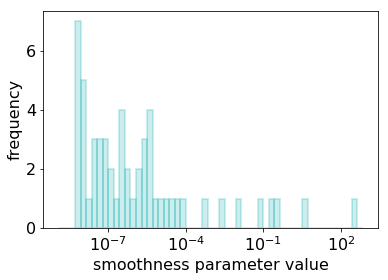
(a) $N/n=5$

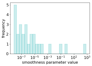
(b) $N/n=10$

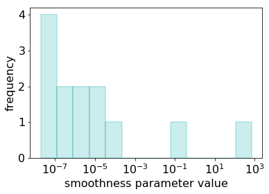
(c) $N/n=20$

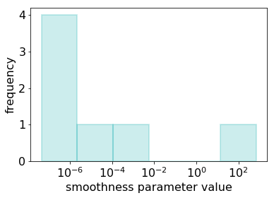
(d) $N/n=40$

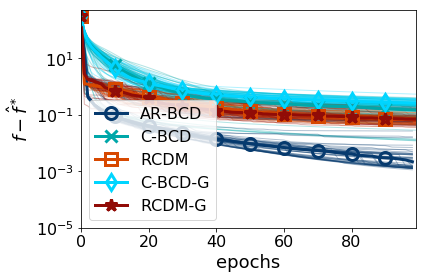
(e) $N/n=5$

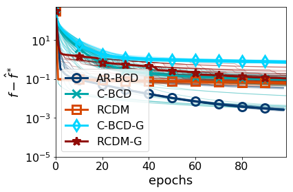
(f) $N/n=10$

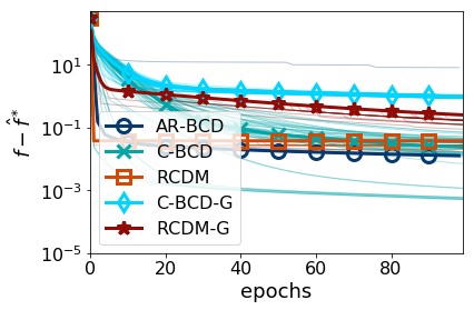
(g) $N/n=20$

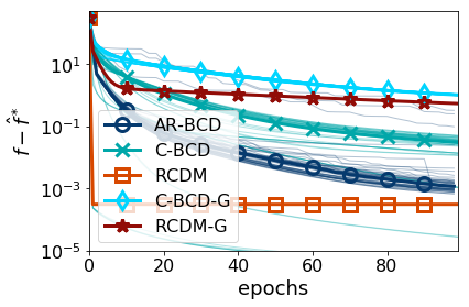
(h) $N/n=40$

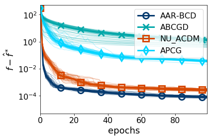
(i) $N/n=5$

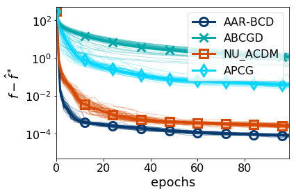
(j) $N/n=10$

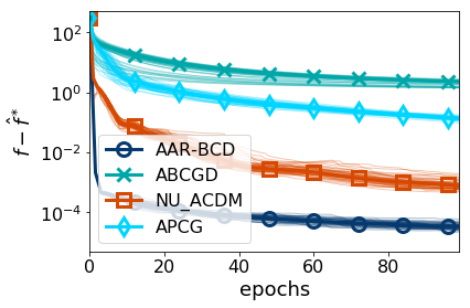
(k) $N/n=20$

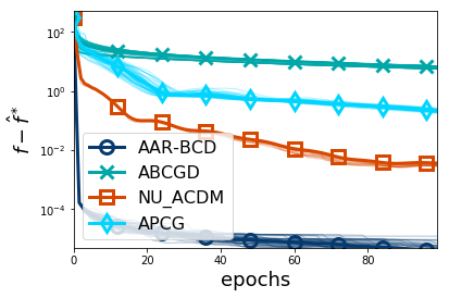
(l) $N/n=40$

Figure 1: Comparison of different block coordinate descent methods: 1(a)-1(d) distribution of smoothness parameters over blocks, 1(e)-1(h) comparison of non-accelerated methods, and 1(i)-1(l) comparison of accelerated methods. Block sizes $N/n$ increase going left to right.

To illustrate the results, we solve the least squares problem on the BlogFeedback Data Set (Buza, 2014) obtained from UCI Machine Learning Repository (Lichman, 2013). The data set contains 280 attributes and 52,396 data points. The attributes correspond to various metrics of crawled blog posts. The data is labeled, and the labels correspond to the number of comments that were posted within 24 hours from a fixed basetime. The goal of a regression method is to predict the number of comments that a blog post receives.

What makes linear regression with least squares on this dataset particularly suitable to our setting is that the smoothness parameters of individual coordinates in the least squares problem take values from a large interval, even when the data matrix $\mathbf{A}$ is scaled by its maximum absolute value (the values are between 0 and $\sim$354). The minimum eigenvalue of $\mathbf{A}^{T}\mathbf{A}$ is zero (i.e., $\mathbf{A}^{T}\mathbf{A}$ is not a full-rank matrix), and thus the problem is not strongly convex.

We partition the data into blocks as follows. We first sort the coordinates by their individual smoothness parameters. Then, we group the first $N/n$ coordinates (from the sorted list of coordinates) into the first block, the second $N/n$ coordinates into the second block, and so on. The chosen block sizes $N/n$ are 5, 10, 20, 40, corresponding to $n=\{56,28,14,7\}$ coordinate blocks, respectively.

The distribution of the smoothness parameters over blocks, for all chosen block sizes, is shown in Fig. 1(a)-1(d). Observe that as the block size increases (going from left to right in Fig. 1(a)-1(d)), the discrepancy between the two largest smoothness parameters increases.

In all the comparisons between the different methods, we define an epoch to be equal to $n$ iterations (this would correspond to a single iteration of a full-gradient method). The graphs plot the optimality gap of the methods over epochs, where the optimal objective value $f^{*}$ is estimated via a higher precision method and denoted by $\hat{f}^{*}$. All the results are shown for 50 method repetitions, with bold lines representing the median optimality gap over those 50 runs. The norm used in all the experiments is $\ell_{2}$, i.e., $\|\cdot\|=\|\cdot\|_{2}$.

Non-accelerated methods

We first compare AR-BCD with a gradient step to RCDM (Nesterov, 2012) and standard cyclic BCD – C-BCD (see, e.g., (Beck & Tetruashvili, 2013)). To make the comparison fair, as AR-BCD makes two steps per iteration, we slow it down by a factor of two compared to the other methods (i.e., we count one iteration of AR-BCD as two). In the comparison, we consider two cases for RCDM and C-BCD: (i) the case in which these two algorithms perform gradient steps on the first $n-1$ blocks and exact minimization on the $n^{\mathrm{th}}$ block (denoted by RCDM and C-BCD in the figure), and (ii) the case in which the algorithms perform gradient steps on all blocks (denoted by RCDM-G and C-BCD-G in the figure). The sampling probabilities for RCDM and AR-BCD are proportional to the block smoothness parameters. The permutation for C-BCD is random, but fixed in each method run.

Fig. 1(e)-1(h) shows the comparison of the described non-accelerated algorithms, for block sizes $N/n\in\{5,10,20,40\}$. The first observation to make is that adding exact minimization over the least smooth block speeds up the convergence of both C-BCD and RCDM, suggesting that the existing analysis of these two methods is not tight. Second, AR-BCD generally converges to a lower optimality gap. While RCDM makes a large initial progress, it stagnates afterwards due to the highly non-uniform sampling probabilities, whereas AR-BCD keeps making progress.

Accelerated methods

Finally, we compare AAR-BCD to NU_ACDM (Allen-Zhu et al., 2016), APCG (Lin et al., 2014), and accelerated C-BCD (ABCGD) from (Beck & Tetruashvili, 2013). As AAR-BCD makes three steps per iteration (as opposed to two steps normally taken by other methods), we slow it down by a factor 1.5 (i.e., we count one iteration of AAR-BCD as 1.5). We chose the sampling probabilities of NU_ACDM and AAR-BCD to be proportional to $\sqrt{L_{i}}$, while the sampling probabilities for APCG are uniform. Similar as before, each full run of ABCGD is performed on a random but fixed permutation of the blocks.

The results are shown in Fig. 1(i)-1(l). Compared to APCG (and ABCGD), NU_ACDM and AAR-BCD converge much faster, which is expected, as the distribution of the smoothness parameters is highly non-uniform and the meethods with non-uniform sampling are theoretically faster by factor of the order $\sqrt{n}$ (Allen-Zhu et al., 2016). As the block size is increased (going left to right), the discrepancy between the smoothness parameters of the least smooth block and the remaining blocks increases, and, as expected, AAR-BCD exhibits more dramatic improvements compared to the other methods.

6 Conclusion

We presented a novel block coordinate descent algorithm AR-BCD and its accelerated version for smooth minimization AAR-BCD. Our work answers the open question of (Beck & Tetruashvili, 2013) whether the convergence of block coordinate descent methods intrinsically depends on the largest smoothness parameter over all the blocks by showing that such a dependence is not necessary, as long as exact minimization over the least smooth block is possible. Before our work, such a result only existed for the setting of two blocks, using the alternating minimization method.

There are several research directions that merit further investigation. For example, we observed empirically that exact optimization over the non-smooth block improves the performance of RCDM and C-BCD, which is not justified by the existing analytical bounds. We expect that in both of these methods the dependence on the least smooth block can be removed, possibly at the cost of a worse dependence on the number of blocks. Further, AR-BCD and AAR-BCD are mainly useful when the discrepancy between the largest block smoothness parameter and the remaining smoothness parameters is large, while under uniform distribution of the smoothness parameters it can be slower than other methods by a factor 1.5-2. It is an interesting question whether there are modifications to AR-BCD and AAR-BCD that would make them uniformly better than the alternatives.

7 Acknowledgements

Part of this work was done while the authors were visiting the Simons Institute for the Theory of Computing. It was partially supported by NSF grant #CCF-1718342 and by the DIMACS/Simons Collaboration on Bridging Continuous and Discrete Optimization through NSF grant #CCF-1740425.

Appendix A Omitted Proofs from Section 4

Proof of Proposition 4.2.

Let $\mathcal{F}_{k-1}$ be the natural filtration up to iteration $k-1$. Observe that, as $\nabla_{n}f(\mathbf{x}_{k})=\mathbf{0}$:

$$\mathbb{E}[\Delta_{k}|\mathcal{F}_{k-1}]=\nabla f(\mathbf{x}_{k}).$$ (A.1)

Since $\mathbf{x}_{1}$ is deterministic (fixed initial point) and the only random variable $\Delta_{1}$ depends on is $i_{1}$, we have:

$$\mathbb{E}[a_{1}\left\langle\Delta_{1},\mathbf{x}_{*}-\mathbf{x}_{1}\right\rangle] =a_{1}\left\langle\nabla f(\mathbf{x}_{1}),\mathbf{x}_{*}-\mathbf{x}_{1}\right\rangle$$ (A.2)

$$=\mathbb{E}[a_{1}\left\langle\nabla f(\mathbf{x}_{1}),\mathbf{x}_{*}-\mathbf{x}_{1}\right\rangle].$$

Let $k>1$. Observe that $a_{j}\left\langle\Delta_{j},\mathbf{x}_{*}-\mathbf{x}_{j}\right\rangle$ is measurable with respect to $\mathcal{F}_{k-1}$ for $j\leq k-1$. By linearity of expectation, using (A.1):

$$\mathbb{E}[\mathop{\textstyle\sum}_{j=1}^{k}a_{j}\left\langle\Delta_{j},\mathbf{x}_{*}-\mathbf{x}_{j}\right\rangle|\mathcal{F}_{k-1}]=a_{k}\left\langle\nabla f(\mathbf{x}_{k}),\mathbf{x}_{*}-\mathbf{x}_{k}\right\rangle+\mathop{\textstyle\sum}_{j=1}^{k-1}a_{j}\left\langle\Delta_{j},\mathbf{x}_{*}-\mathbf{x}_{j}\right\rangle.$$

Taking expectations on both sides of the last equality gives a recursion on $\mathbb{E}[\mathop{\textstyle\sum}_{j=1}^{k}a_{j}\left\langle\Delta_{j},\mathbf{x}_{*}-\mathbf{x}_{j}\right\rangle]$, which, combined with (A.2), completes the proof. ∎

Proof of Lemma 4.5.

As $A_{k-1}\Gamma_{k-1}$ is measurable with respect to the natural filtration $\mathcal{F}_{k-1}$, $\mathbb{E}[A_{k}\Gamma_{k}|\mathcal{F}_{k-1}]\leq A_{k-1}\Gamma_{k-1}$ is equivalent to $\mathbb{E}[A_{k}\Gamma_{k}-A_{k-1}\Gamma_{k-1}|\mathcal{F}_{k-1}]\leq 0$.

The change in the upper bound is:

$$A_{k}U_{k}-A_{k-1}U_{k-1}=A_{k}(f(\mathbf{y}_{k})-f(\mathbf{x}_{k}))+A_{k-1}(f(\mathbf{x}_{k})-f(\mathbf{y}_{k-1}))+a_{k}f(\mathbf{x}_{k}).$$

By convexity, $f(\mathbf{x}_{k})-f(\mathbf{y}_{k-1})\leq\left\langle\nabla f(\mathbf{x}_{k}),\mathbf{x}_{k}-\mathbf{y}_{k-1}\right\rangle$. Further, as $\mathbf{y}_{k}=\mathbf{x}_{k}+I_{N}^{i_{k}}\frac{a_{k}}{p_{i_{k}}A_{k}}(\mathbf{v}_{k}-\mathbf{v}_{k-1})$, we have, by smoothness of $f(\cdot)$, that $f(\mathbf{y}_{k})-f(\mathbf{x}_{k})\leq\left\langle\nabla f(\mathbf{x}_{k}),I_{N}^{i_{k}}\frac{a_{k}}{p_{i_{k}}A_{k}}(\mathbf{v}_{k}-\mathbf{v}_{k-1})\right\rangle+\frac{L_{i_{k}}{a_{k}}^{2}}{2{p_{i_{k}}}^{2}{A_{k}}^{2}}\|\mathbf{v}_{k}^{i_{k}}-\mathbf{v}_{k-1}^{i_{k}}\|^{2}$. Hence:

$$A_{k}U_{k}-A_{k-1}U_{k-1}$$ (A.3)

$$\hskip 28.45274pt\leq a_{k}f(\mathbf{x}_{k})+\left\langle\nabla f(\mathbf{x}_{k}),A_{k-1}(\mathbf{x}_{k}-\mathbf{y}_{k-1})+I_{N}^{i_{k}}\frac{a_{k}}{p_{i_{k}}}(\mathbf{v}_{k}-\mathbf{v}_{k-1})\right\rangle+\frac{L_{i_{k}}{a_{k}}^{2}}{2{p_{i_{k}}}^{2}{A_{k}}}\|\mathbf{v}_{k}^{i_{k}}-\mathbf{v}_{k-1}^{i_{k}}\|^{2}.$$

Let $m_{k}(\mathbf{u})=\sum_{j=1}^{k}a_{j}\left\langle\Delta_{j},\mathbf{u}-\mathbf{x}_{j}\right\rangle+\mathop{\textstyle\sum}_{i=1}^{n}\frac{\sigma_{i}}{2}\|\mathbf{u}^{i}-\mathbf{x}_{1}^{i}\|^{2}$ denote the function under the minimum in the definition of $\Lambda_{k}$. Observe that $m_{k}(\mathbf{u})=m_{k-1}(\mathbf{u})+a_{k}\left\langle\Delta_{k},\mathbf{u}-\mathbf{x}_{k}\right\rangle$ and $\mathbf{v}_{k}=\operatorname*{argmin}_{\mathbf{u}}m_{k}(\mathbf{u})$. Then:

$$m_{k-1}(\mathbf{v}_{k})= m_{k-1}(\mathbf{v}_{k-1})+\left\langle\nabla m_{k-1}(\mathbf{v}_{k-1}),\mathbf{v}_{k}-\mathbf{v}_{k-1}\right\rangle+\mathop{\textstyle\sum}_{i=1}^{n-1}\frac{\sigma_{i}}{2}\|\mathbf{v}_{k}^{i}-\mathbf{v}_{k-1}^{i}\|^{2}$$

$$= m_{k-1}(\mathbf{v}_{k-1})+\frac{\sigma_{i_{k}}}{2}\|\mathbf{v}_{k}^{i_{k}}-\mathbf{v}_{k-1}^{i_{k}}\|^{2},$$

as $\mathbf{v}_{k}$ and $\mathbf{v}_{k-1}$ only differ over the block $i_{k}$ and $\mathbf{v}_{k-1}=\operatorname*{argmin}_{\mathbf{u}}m_{k-1}(\mathbf{u})$ (and, thus, $\nabla m_{k-1}(\mathbf{v}_{k-1})=\mathbf{0}$).

Hence, it follows that $m_{k}(\mathbf{v}_{k})-m_{k-1}(\mathbf{v}_{k-1})=a_{k}\left\langle\Delta_{k},\mathbf{v}_{k}-\mathbf{x}_{k}\right\rangle+\frac{\sigma_{i_{k}}}{2}\|\mathbf{v}_{k}^{i_{k}}-\mathbf{v}_{k-1}^{i_{k}}\|^{2}$, and, thus:

$$A_{k}\Lambda_{k}-A_{k-1}\Lambda_{k-1}=a_{k}f(\mathbf{x}_{k})+a_{k}\left\langle\Delta_{k},\mathbf{v}_{k}-\mathbf{x}_{k}\right\rangle+\frac{\sigma_{i_{k}}}{2}\|\mathbf{v}_{k}^{i_{k}}-\mathbf{v}_{k-1}^{i_{k}}\|^{2}.$$ (A.4)

Combining (A.3) and (A.4):

$$A_{k}\Gamma_{k}-A_{k-1}\Gamma_{k-1}\leq \left\langle\nabla f(\mathbf{x}_{k}),A_{k-1}(\mathbf{x}_{k}-\mathbf{y}_{k-1})+I_{N}^{i_{k}}\frac{a_{k}}{p_{i_{k}}}(\mathbf{v}_{k}-\mathbf{v}_{k-1})\right\rangle-a_{k}\left\langle\Delta_{k},\mathbf{v}_{k}-\mathbf{x}_{k}\right\rangle$$

$$+\frac{L_{i_{k}}{a_{k}}^{2}}{2{p_{i_{k}}}^{2}A_{k}}\|\mathbf{v}_{k}^{i_{k}}-\mathbf{v}_{k-1}^{i_{k}}\|^{2}-\frac{\sigma_{i_{k}}}{2}\|\mathbf{v}_{k}^{i_{k}}-\mathbf{v}_{k-1}^{i_{k}}\|^{2}$$

$$\leq\left\langle\nabla f(\mathbf{x}_{k}),A_{k-1}(\mathbf{x}_{k}-\mathbf{y}_{k-1})+I_{N}^{i_{k}}\frac{a_{k}}{p_{i_{k}}}(\mathbf{v}_{k}-\mathbf{v}_{k-1})\right\rangle-a_{k}\left\langle\Delta_{k},\mathbf{v}_{k}-\mathbf{x}_{k}\right\rangle,$$

as, by the initial assumptions, $\frac{{a_{k}}^{2}}{A_{k}}\leq\frac{p_{i_{k}}^{2}\sigma_{i_{k}}}{L_{i_{k}}}$.

Finally, taking expectations on both sides, and as $\mathbf{x}_{k},\mathbf{y}_{k-1},\mathbf{v}_{k-1}$ are all measurable w.r.t. $\mathcal{F}_{k-1}$ and by the separability of the terms in the definition of $\mathbf{v}_{k}$:

$$\mathbb{E}[A_{k}\Gamma_{k}-A_{k-1}\Gamma_{k-1}|\mathcal{F}_{k-1}]\leq\left\langle\nabla f(\mathbf{x}_{k}),A_{k}\mathbf{x}_{k}-A_{k-1}\mathbf{y}_{k-1}-a_{k}\mathbf{v}_{k-1}\right\rangle=0,$$

as, from (AAR-BCD), $\mathbf{x}_{k}=\mathbf{\hat{x}}_{k}=\frac{A_{k-1}}{A_{k}}\mathbf{y}_{k-1}+\frac{a_{k}}{A_{k}}\mathbf{v}_{k-1}$ over all the blocks except for the block $n,$ while $\nabla_{n}f(\mathbf{x}_{k})=\mathbf{0},$ as $\mathbf{x}_{k}$ is the minimizer of $f$ over block $n,$ when other blocks in $\mathbf{\hat{x}}_{k}$ are fixed. ∎

Appendix B Efficient Implementation of AAR-BCD Iterations

Using similar ideas as in (Fercoq & Richtárik, 2015; Lin et al., 2014; Lee & Sidford, 2013), here we discuss how to efficiently implement iterations of AAR-BCD, without requiring full-vector updates. First, due to the separability of the terms inside the minimum, between successive iterations $\mathbf{v}_{k}$ changes only over a single block. This is formalized in the following simple proposition.

Proposition B.1.

In each iteration $k\geq 1,$ $\mathbf{v}_{k}^{i}=\mathbf{v}_{k-1}^{i}$, $\forall i\neq i_{k}$ and $\mathbf{v}_{k}^{i_{k}}=\mathbf{v}_{k-1}^{i_{k}}+\mathbf{w}^{i_{k}}$, where:

$$\mathbf{w}^{i_{k}}=\operatorname*{argmin}_{\mathbf{u}^{i_{k}}}\{a_{k}\left\langle\Delta_{k}^{i_{k}},\mathbf{u}\right\rangle+\frac{\sigma_{i_{k}}}{2}\|\mathbf{u}^{i_{k}}-\mathbf{v}_{k-1}^{i_{k}}\|^{2}\}.$$

Proof.

Recall the definition of $\mathbf{v}_{k}$. We have:

$$\mathbf{v}_{k}= \operatorname*{argmin}_{\mathbf{u}}\Big{\{}\sum_{j=1}^{k}\left\langle\Delta_{j},\mathbf{u}\right\rangle+\sum_{i=1}^{n-1}\frac{\sigma_{i}}{2}\|\mathbf{u}^{i}-\mathbf{x}_{1}^{i}\|^{2}\Big{\}}$$

$$= \operatorname*{argmin}_{\mathbf{u}}\Big{\{}\sum_{j=1}^{k-1}\left\langle\Delta_{j},\mathbf{u}\right\rangle+\left\langle\Delta_{k},\mathbf{u}\right\rangle+\sum_{i=1}^{n-1}\frac{\sigma_{i}}{2}\|\mathbf{u}^{i}-\mathbf{x}_{1}^{i}\|^{2}\Big{\}}$$

$$= \operatorname*{argmin}_{\mathbf{u}}\Big{\{}\sum_{j=1}^{k-1}\left\langle\Delta_{j},\mathbf{u}\right\rangle+\left\langle\Delta_{k}^{i_{k}},\mathbf{u}^{i_{k}}\right\rangle+\sum_{i=1}^{n-1}\frac{\sigma_{i}}{2}\|\mathbf{u}^{i}-\mathbf{x}_{1}^{i}\|^{2}\Big{\}}$$

$$= \mathbf{v}_{k-1}+\operatorname*{argmin}_{\mathbf{u}^{i_{k}}}\Big{\{}\left\langle\Delta_{k}^{i_{k}},\mathbf{u}^{i_{k}}\right\rangle+\frac{\sigma_{i_{k}}}{2}\|\mathbf{u}^{i_{k}}-\mathbf{v}_{k-1}^{i_{k}}\|^{2}\Big{\}},$$

where the third equality is by the definition of $\Delta_{k}$ ($\Delta_{k}^{i}=0$ for $i\neq i_{k}$) and the last equality follows from block-separability of the terms under the min. ∎

Since $\mathbf{v}_{k}$ only changes over a single block, this will imply that the changes in $\mathbf{x}_{k}$ and $\mathbf{y}_{k}$ can be localized. In particular, let us observe the patterns in changes between successive iterations. We have that, $\forall i\neq n:$

$$\mathbf{x}_{k}^{i} =\frac{A_{k-1}}{A_{k}}\mathbf{y}_{k-1}^{i}+\frac{a_{k}}{A_{k}}\mathbf{v}_{k-1}^{i}=\frac{A_{k-1}}{A_{k}}\left(\mathbf{y}_{k-1}^{i}-\mathbf{v}_{k-1}^{i}\right)+\mathbf{v}_{k-1}^{i}$$ (B.1)

and

$$\mathbf{y}_{k}^{i} =\mathbf{x}_{k}^{i}+\frac{1}{p_{i}}\frac{a_{k}}{A_{k}}\left(\mathbf{v}_{k}^{i}-\mathbf{v}_{k-1}^{i}\right)$$ (B.2)

$$=\frac{A_{k-1}}{A_{k}}\left(\mathbf{y}_{k-1}^{i}-\mathbf{v}_{k-1}^{i}\right)+\left(1-\frac{1}{p_{i}}\frac{a_{k}}{A_{k}}\right)\left(\mathbf{v}_{k-1}^{i}-\mathbf{v}_{k}^{i}\right)+\mathbf{v}_{k}^{i}.$$

Due to Proposition B.1, $\mathbf{v}_{k}$ and $\mathbf{v}_{k-1}$ can be computed without full-vector operations (assuming the gradients can be computed without full-vector operations, which we will show later in this section). Hence, we need to show that it is possible to replace $\frac{A_{k-1}}{A_{k}}\left(\mathbf{y}_{k-1}^{i}-\mathbf{v}_{k-1}^{i}\right)$ with a quantity that can be computed without the full-vector operations. Observe that $\mathbf{y}_{0}-\mathbf{v}_{0}=0$ (from the initialization of (AAR-BCD)) and that, from (B.2):

$$\mathbf{y}_{k}^{i}-\mathbf{v}_{k}^{i}=\frac{A_{k-1}}{A_{k}}\left(\mathbf{y}_{k-1}^{i}-\mathbf{v}_{k-1}^{i}\right)+\left(1-\frac{1}{p_{i}}\frac{a_{k}}{A_{k}}\right)\left(\mathbf{v}_{k-1}^{i}-\mathbf{v}_{k}^{i}\right).$$

Dividing both sides by $\frac{{a_{k}}^{2}}{{A_{k}}^{2}}$ and assuming that $\frac{{a_{k}}^{2}}{A_{k}}$ is constant over iterations, we get:

$$\frac{{A_{k}}^{2}}{{a_{k}}^{2}}\left(\mathbf{y}_{k}^{i}-\mathbf{v}_{k}^{i}\right)=\frac{{A_{k-1}}^{2}}{{a_{k-1}}^{2}}\left(\mathbf{y}_{k-1}^{i}-\mathbf{v}_{k-1}^{i}\right)+\frac{{A_{k}}^{2}}{{a_{k}}^{2}}\left(1-\frac{1}{p_{i}}\frac{a_{k}}{A_{k}}\right)\left(\mathbf{v}_{k-1}^{i}-\mathbf{v}_{k}^{i}\right).$$ (B.3)

Let $N_{n}$ denote the size of the $n^{\mathrm{th}}$ block and define the $(N-N_{n})$-length vector $\mathbf{u}_{k}$ by $\mathbf{u}_{k}^{i}=\frac{{A_{k}}^{2}}{{a_{k}}^{2}}\left(\mathbf{y}_{k}^{i}-\mathbf{v}_{k}^{i}\right)$, $\forall i\neq n$. Then (from (B.3)) $\mathbf{u}_{k}^{i}=\mathbf{u}_{k-1}^{i}+\frac{{A_{k}}^{2}}{{a_{k}}^{2}}\left(1-\frac{1}{p_{i}}\frac{a_{k}}{A_{k}}\right)\left(\mathbf{v}_{k-1}^{i}-\mathbf{v}_{k}^{i}\right),$ and, hence, in iteration $k$, $\mathbf{u}_{k}$ changes only over block $i_{k}$. Combining with (B.1) and (B.2), we have the following lemma.

Lemma B.2.

Assume that $\frac{{a_{k}}^{2}}{A_{k}}$ is kept constant over the iterations of AAR-BCD. Let $\mathbf{u}_{k}$ be the $(N-N_{n})$-dimensional vector defined recursively as $\mathbf{u}_{0}=\mathbf{0}$, $\mathbf{u}_{k}^{i}=\mathbf{u}_{k-1}^{i}$ for $i\in\{1,...,n-1\}$, $i\neq i_{k}$ and $\mathbf{u}_{k}^{i_{k}}=\mathbf{u}_{k-1}^{i_{k}}+\frac{{A_{k}}^{2}}{{a_{k}}^{2}}\left(1-\frac{1}{p_{i}}\frac{a_{k}}{A_{k}}\right)\left(\mathbf{v}_{k-1}^{i}-\mathbf{v}_{k}^{i}\right)$. Then, $\forall i\in\{1,...,n-1\}$: $\mathbf{x}_{k}^{i}=\frac{{a_{k}}^{2}}{{A_{k}}^{2}}\mathbf{u}_{k-1}^{i}+\mathbf{v}_{k-1}^{i}$ and $\mathbf{y}_{k}^{i}=\frac{{a_{k}}^{2}}{{A_{k}}^{2}}\mathbf{u}_{k-1}^{i}+\left(1-\frac{1}{p_{i}}\frac{a_{k}}{A_{k}}\right)\left(\mathbf{v}_{k-1}^{i}-\mathbf{v}_{k}^{i}\right)+\mathbf{v}_{k}^{i}$.

Note that we will never need to explicitly compute $\mathbf{x}_{k},\mathbf{y}_{k}$, except for the last iteration $K$, which outputs $\mathbf{y}_{K}$. To formalize this claim, we need to show that we can compute the gradients $\nabla_{i}f(\mathbf{x}_{k})$ without explicitly computing $\mathbf{x}_{k}$ and that we can efficiently perform the exact minimization over the $n^{\mathrm{th}}$ block. This will only be possible by assuming specific structure of the objective function, as is typical for accelerated block-coordinate descent methods (Fercoq & Richtárik, 2015; Lee & Sidford, 2013; Lin et al., 2014). In particular, we assume that for some $m\times N$ dimensional matrix $\mathbf{M}:$

$$f(\mathbf{x})=\sum_{j=1}^{m}\phi_{j}(e_{j}^{T}\mathbf{M}\mathbf{x})+\psi(\mathbf{x}),$$ (B.4)

where $\phi_{j}:\mathbb{R}\rightarrow\mathbb{R}$ and $\psi=\sum_{i=1}^{n}\psi_{i}:\mathbb{R}^{N}\rightarrow\mathbb{R}$ is block-separable.

Efficient Gradient Computations.

Assume for now that $\mathbf{x}_{k}^{n}$ can be computed efficiently (we will address this at the end of this section). Let ${ind}$ denote the set of indices of the coordinates from blocks $\{1,2,...,n-1\}$ and denote by $\mathbf{B}$ the matrix obtained by selecting the columns of $\mathbf{M}$ that are indexed by ${ind}$. Similarly, let $ind_{n}$ denote the set of indices of the coordinates from block $n$ and let $\mathbf{C}$ denote the submatrix of $\mathbf{M}$ obtained by selecting the columns of $\mathbf{M}$ that are indexed by $ind_{n}$. Denote $\mathbf{r}_{\mathbf{u}_{k}}=\mathbf{B}\mathbf{u}_{k}$, $\mathbf{r}_{\mathbf{v}_{k}}=\mathbf{B}[\mathbf{v}_{k}^{1},\mathbf{v}_{k}^{2},...,\mathbf{v}_{k}^{n-1}]^{T}$, $\mathbf{r}_{n}=\mathbf{C}\mathbf{x}_{k}^{n}$. Let $ind_{i_{k}}$ be the set of indices corresponding to the coordinates from block $i_{k}$. Then:

$$\nabla_{i_{k}}f(\mathbf{x}_{k})=\sum_{j=1}^{m}(\mathbf{M}_{j,ind_{ik}})^{T}\phi_{j}^{\prime}\left(\frac{{a_{k}}^{2}}{{A_{k}}^{2}}\mathbf{r}_{\mathbf{u}_{k-1}}^{j}+\mathbf{r}_{\mathbf{v}_{k-1}}^{j}+\mathbf{r}_{n}^{j}\right)+\nabla_{i_{k}}\psi(\mathbf{x}).$$ (B.5)

Hence, as long as we maintain $\mathbf{r}_{\mathbf{u}_{k}},\mathbf{r}_{\mathbf{v}_{k}},$ and $\mathbf{r}_{n}$ (which do not require full-vector operations), we can efficiently compute the partial gradients $\nabla_{i_{k}}f(\mathbf{x}_{k})$ without ever needing to perform any full-vector operations.

Efficient Exact Minimization.

Suppose first that $\psi(\mathbf{x})\equiv 0$. Then:

$$\mathbf{r}_{n}=\operatorname*{argmin}_{\mathbf{r}\in\mathbb{R}^{m}}\left\{\sum_{j=1}^{m}\phi_{j}\left(\frac{{a_{k}}^{2}}{{A_{k}}^{2}}\mathbf{r}_{\mathbf{u}_{k-1}}^{j}+\mathbf{r}_{\mathbf{v}_{k-1}}^{j}+\mathbf{r}^{j}\right)\right\},$$

and $\mathbf{r}_{n}$ can be computed but solving $m$ single-variable minimization problems, which can be done in closed form or with a very low complexity. Computing $\mathbf{r}_{n}$ is sufficient for defining all algorithm iterations, except for the last one (that outputs a solution). Hence, we only need to compute $\mathbf{x}_{k}^{n}$ once – in the last iteration.

More generally, $\mathbf{x}_{k}^{n}$ is determined by solving:

$$\mathbf{x}_{k}^{n}=\operatorname*{argmin}_{\mathbf{x}\in\mathbb{R}^{N_{n}}}\left\{\sum_{j=1}^{m}\phi_{j}\left(\frac{{a_{k}}^{2}}{{A_{k}}^{2}}\mathbf{r}_{\mathbf{u}_{k-1}}^{j}+\mathbf{r}_{\mathbf{v}_{k-1}}^{j}+(\mathbf{C}\mathbf{x})^{j}\right)+\psi_{n}(\mathbf{x})\right\}.$$

When $m$ and $N_{n}$ are small, high-accuracy polynomial-time convex optimization algorithms are computationally inexpensive, and $\mathbf{x}_{k}^{n}$ can be computed efficiently.

In the special case of linear and ridge regression, $\mathbf{x}_{k}^{n}$ can be computed in closed form, with minor preprocessing. In particular, if $\mathbf{b}$ is the vector of labels, then the problem becomes:

$$\mathbf{x}_{k}^{n}=\operatorname*{argmin}_{\mathbf{x}\in\mathbb{R}^{N_{n}}}\left\{\sum_{j=1}^{m}\left(\frac{{a_{k}}^{2}}{{A_{k}}^{2}}\mathbf{r}_{\mathbf{u}_{k-1}}^{j}+\mathbf{r}_{\mathbf{v}_{k-1}}^{j}+(\mathbf{C}\mathbf{x})^{j}-\mathbf{b}^{j}\right)^{2}+\frac{\lambda}{2}\|\mathbf{x}\|_{2}^{2}\right\},$$

where $\lambda=0$ in the case of (simple) linear regression. Let $\mathbf{b}^{\prime}=\mathbf{b}-\frac{{a_{k}}^{2}}{{A_{k}}^{2}}\mathbf{r}_{\mathbf{u}_{k-1}}-\mathbf{r}_{\mathbf{v}_{k-1}}$. Then:

$$\mathbf{x}_{k}^{n}=(\mathbf{C}^{T}\mathbf{C}+\lambda\mathbf{I})^{\dagger}(\mathbf{C}^{T}\mathbf{b}^{\prime}),$$

where $(\cdot)^{\dagger}$ denotes the matrix pseudoinverse, and $\mathbf{I}$ is the identity matrix. Since $\mathbf{C}^{T}\mathbf{C}+\lambda\mathbf{I}$ does not change over iterations, $(\mathbf{C}^{T}\mathbf{C}+\lambda\mathbf{I})^{\dagger}$ can be computed only once at the initialization. Recall that $\mathbf{C}^{T}\mathbf{C}+\lambda\mathbf{I}$ is an $N_{n}\times N_{n}$ matrix, where $N_{n}$ is the size of the $n^{\mathrm{th}}$ block, and thus inverting $\mathbf{C}^{T}\mathbf{C}+\lambda\mathbf{I}$ is computationally inexpensive as long as $N_{n}$ is not too large. This reduces the overall per-iteration cost of the exact minimization to about the same cost as for performing gradient steps.

References

• Allen-Zhu et al. (2016) Allen-Zhu, Zeyuan, Qu, Zheng, Richtárik, Peter, and Yuan, Yang. Even faster accelerated coordinate descent using non-uniform sampling. In Proc. ICML’16, 2016.
• Beck (2015) Beck, Amir. On the convergence of alternating minimization for convex programming with applications to iteratively reweighted least squares and decomposition schemes. SIAM J. Optimiz., 25(1):185–209, 2015.
• Beck & Tetruashvili (2013) Beck, Amir and Tetruashvili, Luba. On the convergence of block coordinate descent type methods. SIAM J. Optimiz., 23(4):2037–2060, 2013.
• Bertsekas (1999) Bertsekas, Dimitri P. Nonlinear programming. Athena scientific Belmont, 1999.
• Boyd & Vandenberghe (2004) Boyd, Stephen and Vandenberghe, Lieven. Convex optimization. Cambridge university press, 2004.
• Bubeck (2014) Bubeck, Sébastien. Theory of Convex Optimization for Machine Learning. 2014. arXiv preprint, arXiv:1405.4980v1.
• Buza (2014) Buza, Krisztian. Feedback prediction for blogs. In Data analysis, machine learning and knowledge discovery, pp.  145–152. Springer, 2014.
• Diakonikolas & Orecchia (2017) Diakonikolas, Jelena and Orecchia, Lorenzo. The approximate duality gap technique: A unified theory of first-order methods, 2017. arXiv preprint, arXiv:1712.02485.
• Fercoq & Richtárik (2015) Fercoq, Olivier and Richtárik, Peter. Accelerated, parallel, and proximal coordinate descent. SIAM J. Optimiz., 25(4):1997–2023, 2015.
• Gower & Richtárik (2015) Gower, Robert Mansel and Richtárik, Peter. Stochastic dual ascent for solving linear systems. arXiv preprint arXiv:1512.06890, 2015.
• Guminov et al. (2019) Guminov, Sergey, Dvurechensky, Pavel, and Gasnikov, Alexander. Accelerated alternating minimization. arXiv preprint arXiv:1906.03622, 2019.
• Hampel et al. (2011) Hampel, Frank R, Ronchetti, Elvezio M, Rousseeuw, Peter J, and Stahel, Werner A. Robust statistics: the approach based on influence functions, volume 196. John Wiley & Sons, 2011.
• Lee & Sidford (2013) Lee, Yin Tat and Sidford, Aaron. Efficient accelerated coordinate descent methods and faster algorithms for solving linear systems. In Proc. IEEE FOCS’13, 2013.
• Lichman (2013) Lichman, M. UCI machine learning repository, 2013. URL http://archive.ics.uci.edu/ml.
• Lin et al. (2014) Lin, Qihang, Lu, Zhaosong, and Xiao, Lin. An accelerated proximal coordinate gradient method. In Proc. NIPS’14, 2014.
• Nesterov (2012) Nesterov, Yu. Efficiency of coordinate descent methods on huge-scale optimization problems. SIAM J. Optimiz., 22(2):341–362, 2012.
• Nesterov & Stich (2017) Nesterov, Yurii and Stich, Sebastian U. Efficiency of the accelerated coordinate descent method on structured optimization problems. SIAM J. Optimiz., 27(1):110–123, 2017.
• Ortega & Rheinboldt (1970) Ortega, James M and Rheinboldt, Werner C. Iterative solution of nonlinear equations in several variables, volume 30. SIAM, 1970.
• Qu & Richtárik (2016) Qu, Zheng and Richtárik, Peter. Coordinate descent with arbitrary sampling i: Algorithms and complexity. Optimization Methods and Software, 31(5):829–857, 2016.
• Qu et al. (2016) Qu, Zheng, Richtárik, Peter, Takáč, Martin, and Fercoq, Olivier. SDNA: Stochastic dual Newton ascent for empirical risk minimization. In Proc. ICML’16, 2016.
• Richtárik & Takáč (2014) Richtárik, Peter and Takáč, Martin. Iteration complexity of randomized block-coordinate descent methods for minimizing a composite function. Math. Prog., 144(1-2):1–38, 2014.
• Saha & Tewari (2013) Saha, Ankan and Tewari, Ambuj. On the nonasymptotic convergence of cyclic coordinate descent methods. SIAM J. Optimiz., 23(1):576–601, 2013.
• Strohmer & Vershynin (2009) Strohmer, Thomas and Vershynin, Roman. A Randomized Kaczmarz Algorithm with Exponential Convergence. J. Fourier Anal. Appl., 15(2):262–278, 2009.
• Sun & Hong (2015) Sun, Ruoyu and Hong, Mingyi. Improved iteration complexity bounds of cyclic block coordinate descent for convex problems. In Proc. NIPS’15, 2015.
• Tseng & Yun (2009) Tseng, Paul and Yun, Sangwoon. A coordinate gradient descent method for nonsmooth separable minimization. Math. Prog., 117(1-2):387–423, 2009.
• Wright (2015) Wright, Stephen J. Coordinate descent algorithms. Math. Prog., 151(1):3–34, 2015.