A Transition-based Algorithm for Unrestricted AMR Parsing

Abstract

Non-projective parsing can be useful to handle cycles and reentrancy in amr graphs. We explore this idea and introduce a greedy left-to-right non-projective transition-based parser. At each parsing configuration, an oracle decides whether to create a concept or whether to connect a pair of existing concepts. The algorithm handles reentrancy and arbitrary cycles natively, i.e. within the transition system itself. The model is evaluated on the LDC2015E86 corpus, obtaining results close to the state of the art, including a Smatch of 64%, and showing good behavior on reentrant edges.

1 Introduction

Abstract Meaning Representation (amr) is a semantic representation language to map the meaning of English sentences into directed, cycled, labeled graphs Banarescu et al. (2013). Graph vertices are concepts inferred from words. The concepts can be represented by the words themselves (e.g. dog), PropBank framesets Palmer et al. (2005) (e.g. eat-01), or keywords (like named entities or quantities). The edges denote relations between pairs of concepts (e.g. eat-01 :ARG0 dog). amr parsing integrates tasks that have usually been addressed separately in natural language processing (nlp), such as named entity recognition Nadeau and Sekine (2007), semantic role labeling Palmer et al. (2010) or co-reference resolution Ng and Cardie (2002); Lee et al. (2017). Figure 1 shows an example of an amr graph.

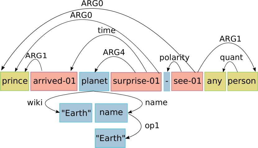
Figure 1: amr graph for ‘When the prince arrived on the Earth, he was surprised not to see any people’. Words can refer to concepts by themselves (green), be mapped to PropBank framesets (red) or be broken down into multiple-term/non-literal concepts (blue). Prince plays different semantic roles.

Several transition-based dependency parsing algorithms have been extended to generate amr. Wang et al. (2015) describe a two-stage model, where they first obtain the dependency parse of a sentence and then transform it into a graph. Damonte et al. (2017) propose a variant of the arc-eager algorithm to identify labeled edges between concepts. These concepts are identified using a lookup table and a set of rules. A restricted subset of reentrant edges are supported by an additional classifier. A similar configuration is used in Gildea et al. (2018); Peng et al. (2018), but relying on a cache data structure to handle reentrancy, cycles and restricted non-projectivity. A feed-forward network and additional hooks are used to build the concepts. Ballesteros and Al-Onaizan (2017) use a modified arc-standard algorithm, where the oracle is trained using stack-lstms Dyer et al. (2015). Reentrancy is handled through swap Nivre (2009) and they define additional transitions intended to detect concepts, entities and polarity nodes.

This paper explores unrestricted non-projective amr parsing and introduces amr-covington, inspired by Covington (2001). It handles arbitrary non-projectivity, cycles and reentrancy in a natural way, as there is no need for specific transitions, but just the removal of restrictions from the original algorithm. The algorithm has full coverage and keeps transitions simple, which is a matter of concern in recent studies Peng et al. (2018).

2 Preliminaries and Notation

Notation

We use typewriter font for concepts and their indexes (e.g. dog or 1), regular font for raw words (e.g. dog or 1), and a bold style font for vectors and matrices (e.g. $\mathbf{v}$, $\mathbf{W}$).

Covington (2001) describes a fundamental algorithm for unrestricted non-projective dependency parsing. The algorithm can be implemented as a left-to-right transition system Nivre (2008). The key idea is intuitive. Given a word to be processed at a particular state, the word is compared against the words that have previously been processed, deciding to establish or not a syntactic dependency arc from/to each of them. The process continues until all previous words are checked or until the algorithm decides no more connections with previous words need to be built, then the next word is processed. The runtime is $\mathcal{O}(n^{2})$ in the worst scenario. To guarantee the single-head and acyclicity conditions that are required in dependency parsing, explicit tests are added to the algorithm to check for transitions that would break the constraints. These are then disallowed, making the implementation less straightforward.

3 The amr-Covington algorithm

The acyclicity and single-head constraints are not needed in amr, as arbitrary graphs are allowed. Cycles and reentrancy are used to model semantic relations between concepts (as shown in Figure 1) and to identify co-references. By removing the constraints from the Covington transition system, we achieve a natural way to deal with them.

Also, amr parsing requires words to be transformed into concepts. Dependency parsing operates on a constant-length sequence. But in amr, words can be removed, generate a single concept, or generate several concepts. In this paper, additional lookup tables and transitions are defined to create concepts when needed, following the current trend Damonte et al. (2017); Ballesteros and Al-Onaizan (2017); Gildea et al. (2018).

3.1 Formalization

Let $G$=$(V,E)$ be an edge-labeled directed graph where: $V$=$\{\texttt{0},\texttt{1},\texttt{2},\ldots,\texttt{M}\}$ is the set of concepts and $E=V\times E\times V$ is the set of labeled edges, we will denote a connection between a head concept $\texttt{i}\in V$ and a dependent concept $\texttt{j}\in V$ as $\texttt{i}\xrightarrow{l}\texttt{j}$, where l is the semantic label connecting them.

The parser will process sentences from left to right. Each decision leads to a new parsing configuration, which can be abstracted as a 4-tuple $(\lambda_{1},\lambda_{2},\beta,E)$ where:

• $\beta$ is a buffer that contains unprocessed words. They await to be transformed to a concept, a part of a larger concept, or to be removed. In $b|\beta$, $b$ represents the head of $\beta$, and it optionally can be a concept. In that case, it will be denoted as b.

• $\lambda_{1}$ is a list of previously created concepts that are waiting to determine its semantic relation with respect to b. Elements in $\lambda_{1}$ are concepts. In $\lambda_{1}|\texttt{i}$, i denotes its last element.

• $\lambda_{2}$ is a list that contains previously created concepts for which the relation with b has already been determined. Elements in $\lambda_{2}$ are concepts. In $\texttt{j}|\lambda_{2}$, j denotes the head of $\lambda_{2}$.

• $E$ is the set of the created edges.

Transitions	Step $t$	Step $t+1$
left-arcl	$(\lambda_{1}|\texttt{i},\lambda_{2},\texttt{b}|\beta,E)$	$(\lambda_{1},\texttt{i}|\lambda_{2},\texttt{b}|\beta,E\cup\{\texttt{b}\xrightarrow{l}\texttt{i}\})$
right-arcl	$(\lambda_{1}|\texttt{i},\lambda_{2},\texttt{b}|\beta,E)$	$(\lambda_{1},\texttt{i}|\lambda_{2},\texttt{b}|\beta,E\cup\{\texttt{i}\xrightarrow{l}\texttt{b}\})$
multiple-arc${}_{l_{1},l_{2}}$	$(\lambda_{1}|\texttt{i},\lambda_{2},\texttt{b}|\beta,E)$	$(\lambda_{1},\texttt{i}|\lambda_{2},\texttt{b}|\beta,E\cup\{\texttt{b}\xrightarrow{l}\texttt{i}\}\cup\{\texttt{i}\xrightarrow{l_{2}}\texttt{b}\})$
shift	$(\lambda_{1},\lambda_{2},\texttt{b}|\beta,E)$	$(\lambda_{1}\cdot\lambda_{2}|\texttt{b},[],\beta,E)$
no-arc	$(\lambda_{1}|\texttt{i},\lambda_{2},\beta,E)$	$(\lambda_{1},\texttt{i}|\lambda_{2},\beta,E)$
confirm	$(\lambda_{1},\lambda_{2},b|\beta,E)$	$(\lambda_{1},\lambda_{2},\texttt{b}|\beta,E)$
breakdownα	$(\lambda_{1},\lambda_{2},b|\beta,E)$	$(\lambda_{1},\lambda_{2},\texttt{b}|b|\beta,E)$
reduce	$(\lambda_{1},\lambda_{2},b|\beta,E)$	$(\lambda_{1},\lambda_{2},\beta,E)$

Table 1: Transitions for amr-covington

Given an input sentence, the parser starts at an initial configuration $c_{s}$ = $([\texttt{0}],[],1|\beta,\{\})$ and will apply valid transitions until a final configuration $c_{f}$ is reached, such that $c_{f}$ = $(\lambda_{1},\lambda_{2},[],E)$. The set of transitions is formally defined in Table 1:

• left-arc_l: Creates an edge $\texttt{b}\xrightarrow{l}\texttt{i}$. i is moved to $\lambda_{2}$.

• right-arc_l: Creates an edge $\texttt{i}\xrightarrow{l}\texttt{b}$. i is moved to $\lambda_{2}$.

• shift: Pops b from $\beta$. $\lambda_{1}$, $\lambda_{2}$ and b are appended.

• no arc: It is applied when the algorithm determines that there is no semantic relationship between i and b, but there is a relationship between some other node in $\lambda_{1}$ and b.

• confirm: Pops $b$ from $\beta$ and puts the concept b in its place. This transition is called to handle words that only need to generate one (more) concept.

• breakdown_α: Creates a concept b from $b$, and places it on top of $\beta$, but $b$ is not popped, and the new buffer state is $\texttt{b}|b|\beta$. It is used to handle a word that is going to be mapped to multiple concepts. To guarantee termination, breakdown is parametrized with a constant $\alpha$, banning generation of more than $\alpha$ consecutive concepts by using this operation. Otherwise, concepts could be generated indefinitely without emptying $\beta$.

• reduce: Pops $b$ from $\beta$. It is used to remove words that do not add any meaning to the sentence and are not part of the amr graph.

left and right-arc handle cycles and reentrancy with the exception of cycles of length 2 (which only involve i and b). To assure full coverage, we include an additional transition: multiple-arc${}_{(l_{1},l_{2})}$ that creates two edges $\texttt{b}\xrightarrow{l_{1}}\texttt{i}$ and $\texttt{i}\xrightarrow{l_{2}}\texttt{b}$. i is moved to $\lambda_{2}$. multiple-arcs are marginal and will not be learned in practice. amr-covington can be implemented without multiple-arc, by keeping i in $\lambda_{1}$ after creating an arc and using no-arc when the parser has finished creating connections between i and b, at a cost to efficiency as transition sequences would be longer. Multiple edges in the same direction between i and b are handled by representing them as a single edge that merges the labels.

Example

Table 2 illustrates a valid transition sequence to obtain the amr graph of Figure 1.

$\mathbf{\lambda_{1}}$	$\mathbf{\lambda_{2}}$	$\mathbf{\beta}$	Action (times)
		w, t, p	reduce$\times 2_{1}$
		p, a, o	confirm2
		p, a, o	shift3
p		a, o, t	confirm4
p		a, o, t	left-arc5
	p	a, o, t	shift6
p, a		o, t, E	reduce$\times 2_{7}$
p, a		E, h, w	breakdown8
p, a		‘E’, E, h	shift9
p, a, ‘E’		E, h, w	breakdown10
p, a, ‘E’		‘E’, h, w	shift11
a, ‘E’, ‘E’		E, h, w	breakdown12
a, ‘E’, ‘E’		n, h, w	left-arc12
a, ‘E’	‘E’	n, h, w	shift13
‘E’, ‘E’, n		E, h, w	confirm14
‘E’, ‘E’, n		p2, h, w	left-arc15
a, ‘E’, ‘E’	n,	p2, h, w	no-arc16
p, a, ‘E’	‘E’, n,	p2, h, w	left-arc17
p, a	‘E’, ‘E’, n,	p2, h, w	shift18
‘E’, n, p2		h, w, s	reduce$\times 2_{19}$
‘E’, n, p2		s, n, t	confirm20
‘E’, n, p2		s, n, t	left-arc21
‘E’, ‘E’, n	p2	s, n, t	no-arc$\times 3_{22}$
p, a	‘E’, ‘E’, n	s, n, t	left-arc$\times 2_{23}$
	p, a, ‘E’	s, n, t	shift24
n, p2, s		n, t, s2	confirm25
n, p2, s		-, t, s2	shift26
p2, s, -		t, s2, a2	reduce27
p2, s, -		s2, a2, p3	confirm28
p2, s, -		s2, a2, p3	left-arc29
n, p2, s	-	s2, a2, p3	no-arc $\times 5_{30}$
p	a, ‘E’, ‘E’	s2, a2, p3	left-arc31
	p, a, ‘E’	s2, a2, p3	shift32
s, -, s2		a2, p3	confirm33
s, -, s2		a2, p3	shift34
-, s2, a2		p3	confirm35
-, s2, a2		p3	left-arc36
s, -, s2	a2	p3	right-arc37
s2, a2, p3			shift38

Table 2: Sequence of gold transitions to obtain the amr graph for the sentence ‘When the prince arrived on the Earth, he was surprised not to see any people’, introduced in Figure 1. For brevity, we represent words (and concepts) by their first character (plus an index if it is duplicated) and we only show the top three words for $\lambda_{1}$, $\lambda_{2}$ and $\beta$. Steps from 20 to 23(2) and from 28 to 31 manage the reentrant edges for prince (p) from surprise-01 (s) and see-01 (s2).

3.2 Training the classifiers

The algorithm relies on three classifiers: (1) a transition classifier, $T_{c}$, that learns the set of transitions introduced in §3.1, (2) a relation classifier, $R_{c}$, to predict the label(s) of an edge when the selected action is a left-arc, right-arc or multiple-arc and (3) a hybrid process (a concept classifier, $C_{c}$, and a rule-based system) that determines which concept to create when the selected action is a confirm or breakdown.

Preprocessing

Sentences are tokenized and aligned with the concepts using Jamr Flanigan et al. (2014). For lemmatization, tagging and dependency parsing we used UDpipe Straka et al. (2016) and its English pre-trained model Zeman et al. (2017). Named Entity Recognition is handled by Stanford CoreNLP Manning et al. (2014).

Architecture

We use feed-forward neural networks to train the tree classifiers. The transition classifier uses 2 hidden layers (400 and 200 input neurons) and the relation and concept classifiers use 1 hidden layer (200 neurons). The activation function in hidden layers is a $relu(x)$=$max(0,x)$ and their output is computed as $relu(W_{i}\cdot\mathbf{x}_{i}+b_{i})$ where $W_{i}$ and $b_{i}$ are the weights and bias tensors to be learned and $\mathbf{x}_{i}$ the input at the $i$th hidden layer. The output layer uses a $\mathit{softmax}$ function, computed as $P(y=s|\mathbf{x})=\frac{e^{\mathbf{x^{T}}\theta_{s}}}{\sum_{s^{\prime}=1}^{S}e^{\mathbf{x^{T}}\theta_{s^{\prime}}}}$. All classifiers are trained in mini-batches (size=32), using Adam Kingma and Ba (2015) (learning rate set to $3e^{-4}$), early stopping (no patience) and dropout Srivastava et al. (2014) (40%). The classifiers are fed with features extracted from the preprocessed texts. Depending on the classifier, we are using different features. These are summarized in Appendix A (Table 5), which also describes (B) other design decisions that are not shown here due to space reasons.

3.3 Running the system

At each parsing configuration, we first try to find a multiword concept or entity that matches the head elements of $\beta$, to reduce the number of breakdowns, which turned out to be a difficult transition to learn (see §4.1). This is done by looking at a lookup table of multiword concepts seen in the training set and a set of rules, as introduced in Damonte et al. (2017); Gildea et al. (2018).

We then invoke $T_{c}$ and call the corresponding subprocess when an additional concept or edge-label identification task is needed.

Concept identification

If the word at the top of $\beta$ occurred more than 4 times in the training set, we call a supervised classifier to predict the concept. Otherwise, we first look for a word-to-concept mapping in a lookup table. If not found, if it is a verb, we generate the concept lemma-01, and otherwise lemma.

Edge label identification

The classifier is invoked every time an edge is created. We use the list of valid ARGs allowed in propbank framesets by Damonte et al. (2017). Also, if p and o are a propbank and a non-propbank concept, we restore inverted edges of the form o $\xrightarrow{\texttt{l-of}}$ p as o $\xrightarrow{\texttt{l}}$ p.

4 Methods and Experiments

Corpus

We use the LDC2015E86 corpus and its official splits: 16 833 graphs for training, 1 368 for development and 1 371 for testing. The final model is only trained on the training split.

Metrics

We use Smatch Cai and Knight (2013) and the metrics from Damonte et al. (2017).

Sources

The code and the pretrained model used in this paper can be found at https://github.com/aghie/tb-amr.

4.1 Results and discussion

Table 3 shows accuracy of $T_{c}$ on the development set. confirm and reduce are the easiest transitions, as local information such as POS-tags and words are discriminative to distinguish between content and function words. breakdown is the hardest action. In early stages of this work, we observed that this transition could learn to correctly generate multiple-term concepts for named-entities that are not sparse (e.g. countries or people), but failed with sparse entities (e.g. dates or percent quantities). Low performance on identifying them negatively affects the edge metrics, which require both concepts of an edge to be correct. Because of this and to identify them properly, we use the mentioned complementary rules to handle named entities. right-arcs are harder than left-arcs, although the reason for this issue remains as an open question for us. The performance for no-arcs is high, but it would be interesting to achieve a higher recall at a cost of a lower precision, as predicting no-arcs makes the transition sequence longer, but could help identify more distant reentrancy. The accuracy of $T_{c}$ is $\sim$86%. The accuracy of $R_{c}$ is $\sim$79%. We do not show the detailed results since the number of classes is too high. $C_{c}$ was trained on concepts occurring more than 1 time in the training set, obtaining an accuracy of $\sim$83%. The accuracy on the development set with all concepts was $\sim$77%.

Action	Prec.	Rec.	F-score
left-arc	81.62	87.73	84.57
right-arc	75.53	78.71	77.08
multiple-arc	00.00	00.00	00.00
shift	80.44	81.11	80.77
no-arc	89.71	86.71	88.18
confirm	84.91	96.11	90.16
reduce	96.77	91.53	94.08
breakdown	85.09	50.23	63.17

Table 3: $T_{c}$ scores on the development set.

Table 4 compares the performance of our systems with state-of-the-art models on the test set. amr-covington obtains state-of-the-art results for all the standard metrics. It outperforms the rest of the models when handling reentrant edges. It is worth noting that D requires an additional classifier to handle a restricted set of reentrancy and P uses up to five classifiers to build the graph.

Metric	F	W	F’	D	P	Ours
Smatch	58	63	67	64	64	64
Unlabeled	61	69	69	69	-	68
No-WSD	58	64	68	65	-	65
NER	75	75	79	83	-	83
Wiki	0	0	75	64	-	70
Negations	16	18	45	48	-	47
Concepts	79	80	83	83	-	83
Reentrancy	38	41	42	41	-	44
SRL	55	60	60	56	-	57

Table 4: F-score comparison with F Flanigan et al. (2014), W Wang et al. (2015), F’ Flanigan et al. (2016), D Damonte et al. (2017), P Peng et al. (2018). D, P and our system are left-to-right transition-based.

Discussion

In contrast to related work that relies on ad-hoc procedures, the proposed algorithm handles cycles and reentrant edges natively. This is done by just removing the original constraints of the arc transitions in the original Covington (2001) algorithm. The main drawback of the algorithm is its computational complexity. The transition system is expected to run in $\mathcal{O}(n^{2})$, as the original Covington parser. There are also collateral issues that impact the real speed of the system, such as predicting the concepts in a supervised way, given the large number of output classes (discarding the less frequent concepts the classifier needs to discriminate among more than 7 000 concepts). In line with previous discussions Damonte et al. (2017), it seems that using a supervised feed-forward network to predict the concepts does not lead to a better overall concept identification with respect of the use of simple lookup tables that pick up the most common node/subgraph. Currently, every node is kept in $\lambda$, and it is available to be part of new edges. We wonder if only storing in $\lambda$ the head node for words that generate multiple-node subgraphs (e.g. for the word father that maps to have-rel-role-91 :ARG2 father, keeping in $\lambda$ only the concept have-rel-role-91) could be beneficial for amr-covington.

As a side note, current amr evaluation involves elements such as neural network initialization, hooks and the (sub-optimal) alignments of evaluation metrics (e.g. Smatch) that introduce random effects that were difficult to quantify for us.

5 Conclusion

We introduce amr-covington, a non-projective transition-based parser for unrestricted amr. The set of transitions handles reentrancy natively. Experiments on the LDC2015E86 corpus show that our approach obtains results close to the state of the art and a good behavior on re-entrant edges.

As future work, amr-covington produces sequences of no-arcs which could be shortened by using non-local transitions Qi and Manning (2017); Fernández-González and Gómez-Rodríguez (2017). Sequential models have shown that fewer hooks and lookup tables are needed to deal with the high sparsity of amr Ballesteros and Al-Onaizan (2017). Similarly, bist-covington Vilares and Gómez-Rodríguez (2017) could be adapted for this task.

Appendix A Supplemental Material

Table 5 indicates the features used to train the different classifiers. Concept features are randomized by $\epsilon=2e^{-3}$ to an special index that refers to an unknown concept during the training phase. This helps learn a generic embedding for unseen concepts in the test phase. Also, concepts that occur only one time in the training set are not considered as output classes by $C_{c}$.

Features	$T_{c}$	$R_{c}$	$C_{c}$
From $\beta_{0},\beta_{1},\lambda_{1_{0}},\lambda_{1_{1}}$
pos	✓	✓	✓
w	✓	✓	✓
ew	✓	✓	✓
c	✓	✓	✓
entity	✓	✓	✓
lmh	✓	✓
lmc	✓	✓
lmcc	✓	✓
rmh	✓	✓
rmc	✓	✓
rmcc	✓	✓
nh, nc	✓	✓
depth	✓	✓	✓
npunkt	✓	✓
hl	✓	✓
ct	✓	✓
g			✓
Labels from the predicted
dependency tree
d$(b_{j},i_{k})\ \forall j,k\ j\in[0,1]$	✓	✓	✓
$\wedge\ k\in[0,1,2,3]$

Table 5: Set of proposed features for each classifier. pos, w, c, entity are part-of-speech tag, word, concept and entity embeddings. ew are pre-trained external word embeddings, fine-tuned during the training phase (http://nlp.stanford.edu/data/glove.6B.zip, 100 dimensions). lm and rm are the leftmost and the rightmost function; and h, c, cc represent head, child and grand-child concepts of a concept; so, for example, lm_c stands for the leftmost child of the concept. nh and nc are the number of heads and children of a concept. npunkt indicates the number of ‘.’, ‘;’, ‘:’, ‘?’, ‘!’ that have already been processed. hl denotes the labels of the last assigned head. ct indicates the type of concept (constant, propbank frameset, other). g indicates if a concept was generated using a confirm or breakdown. d denotes the dependency label existing in the dependency tree between the word at the $j$th position in $\beta$ and the $k$th last in $\lambda_{1}$ and vice versa. The word that generated a concept is still accessible after creating the concept.

Internal and external (from GloVe) word embedding sizes are set to 100. The size of the concept embedding is set to 50. The rest of the embeddings size are set to 20. The weights are initialized to zero.

Appendix B Additional design decisions

We try to list more in detail the main hooks and design decisions followed in this work to mitigate the high sparsity in Abstract Meaning Representation which, at least in our experience, was a struggling issue. These decisions mainly affect the mapping from words to multiple-concept subgraphs.

• We identify named entities and nationalities, and update the training configurations to generate the corresponding subgraph by applying a set of hooks. The intermediate training configurations are not fed as samples to the classifier. On early experiments it was observed that the breakdown transition could acceptably learn non-sparse named entities (e.g. countries and nationalities), but failed on the sparse ones (e.g. dates or money amounts). By processing the named entities with hooks instead, the aim was to make the parser familiar with the parsing configurations that are obtained after applying the hooks.

• Additionally, named-entity subgraphs and subgraphs coming from phrases (involving two or more terms) from the training set are saved into a lookup table. The latter ones had little impact.

• We store in a lookup table some single-word expressions that generated multiple-concept subgraphs in the training set, based on simple heuristics. We store words that denote a negative expression (e.g. undecided that maps to decide-01 :polarity -). We store words that always generated the same subgraph and occurred more than 5 times. We also store capitalized single words that were not previously identified as named entities.

• We use the verbalization list from Wang et al. (2015) (another lookup table).

• When predicting a confirm or breakdown for an uncommon word, we check if that word was mapped to a concept in the training set. If not, we generate the concept lemma-01 if it is a verb, otherwise lemma.

• Dates formatted as YYMMDD or YYYYMMDD are identified using a simple criterion (sequence of 6 or 8 digits) and transformed into YYYY-MM-DD on the test phase, as they were consistently misclassified as integer numbers in the development set.

• We apply a set of hooks similar to Damonte et al. (2017) to determine if the predicted label is valid for that edge.

• We forbid to generate the same concept twice consecutively. Also, we set $\alpha=4$ for breakdown_α.

• If a node is created, but it is not attached to any head node, we post-process it and connect to the root node.

• We assume multi-sentence graphs should contain sentence punctuation symbols. If we predict a multi-sentence graph, but there is no punctuation symbol that splits sentences, we post-process the graph and transform the root node into an and node.

References

- Ballesteros and Al-Onaizan (2017) Miguel Ballesteros and Yaser Al-Onaizan. 2017. AMR Parsing using Stack-LSTMs. In Proceedings of the 2017 Conference on Empirical Methods in Natural Language Processing, pages 1280–1286, Copenhagen, Denmark. Association for Computational Linguistics.
- Banarescu et al. (2013) Laura Banarescu, Claire Bonial, Shu Cai, Madalina Georgescu, Kira Griffitt, Ulf Hermjakob, Kevin Knight, Philipp Koehn, Martha Palmer, and Nathan Schneider. 2013. Abstract meaning representation for sembanking. In Proceedings of the 7th Linguistic Annotation Workshop and Interoperability with Discourse, pages 178–186.
- Cai and Knight (2013) Shu Cai and Kevin Knight. 2013. Smatch: an Evaluation Metric for Semantic Feature Structures. In ACL (2), pages 748–752.
- Covington (2001) Michael A Covington. 2001. A fundamental algorithm for dependency parsing. In Proceedings of the 39th annual ACM southeast conference, pages 95–102.
- Damonte et al. (2017) Marco Damonte, Shay B. Cohen, and Giorgio Satta. 2017. An Incremental Parser for Abstract Meaning Representation. In Proceedings of the 15th Conference of the European Chapter of the Association for Computational Linguistics: Volume 1, Long Papers, pages 536–546, Valencia, Spain. Association for Computational Linguistics.
- Dyer et al. (2015) Chris Dyer, Miguel Ballesteros, Wang Ling, Austin Matthews, and Noah A. Smith. 2015. Transition-Based Dependency Parsing with Stack Long Short-Term Memory. In Proceedings of the 53rd Annual Meeting of the Association for Computational Linguistics and the 7th International Joint Conference on Natural Language Processing (Volume 1: Long Papers), pages 334–343, Beijing, China. Association for Computational Linguistics.
- Fernández-González and Gómez-Rodríguez (2017) D. Fernández-González and C. Gómez-Rodríguez. 2017. Non-Projective Dependency Parsing with Non-Local Transitions. ArXiv e-prints.
- Flanigan et al. (2016) Jeffrey Flanigan, Chris Dyer, Noah A Smith, and Jaime Carbonell. 2016. CMU at SemEval-2016 task 8: Graph-based AMR Parsing with Infinite Ramp Loss. In Proceedings of the 10th International Workshop on Semantic Evaluation (SemEval-2016), pages 1202–1206.
- Flanigan et al. (2014) Jeffrey Flanigan, Sam Thomson, Jaime Carbonell, Chris Dyer, and Noah A. Smith. 2014. A Discriminative Graph-Based Parser for the Abstract Meaning Representation. In Proceedings of the 52nd Annual Meeting of the Association for Computational Linguistics (Volume 1: Long Papers), pages 1426–1436, Baltimore, Maryland. Association for Computational Linguistics.
- Gildea et al. (2018) Daniel Gildea, Giorgio Satta, and Xiaochang Peng. 2018. Cache Transition Systems for Graph Parsing. Computational Linguistics, in press.
- Kingma and Ba (2015) Diederik Kingma and Jimmy Ba. 2015. Adam: A method for stochastic optimization. In Proceedings of the 3rd International Conference for Learning Representations, San Diego, USA.
- Lee et al. (2017) Heeyoung Lee, Mihai Surdeanu, and Dan Jurafsky. 2017. A scaffolding approach to coreference resolution integrating statistical and rule-based models. Natural Language Engineering, pages 1–30.
- Manning et al. (2014) Christopher D. Manning, Mihai Surdeanu, John Bauer, Jenny Finkel, Steven J. Bethard, and David McClosky. 2014. The Stanford CoreNLP natural language processing toolkit. In Association for Computational Linguistics (ACL) System Demonstrations, pages 55–60.
- Nadeau and Sekine (2007) David Nadeau and Satoshi Sekine. 2007. A survey of named entity recognition and classification. Lingvisticae Investigationes, 30(1):3–26.
- Ng and Cardie (2002) Vincent Ng and Claire Cardie. 2002. Improving machine learning approaches to coreference resolution. In Proceedings of the 40th annual meeting on association for computational linguistics, pages 104–111. Association for Computational Linguistics.
- Nivre (2008) Joakim Nivre. 2008. Algorithms for deterministic incremental dependency parsing. Computational Linguistics, 34(4):513–553.
- Nivre (2009) Joakim Nivre. 2009. Non-projective dependency parsing in expected linear time. In Proceedings of the Joint Conference of the 47th Annual Meeting of the ACL and the 4th International Joint Conference on Natural Language Processing of the AFNLP: Volume 1-Volume 1, pages 351–359. Association for Computational Linguistics.
- Palmer et al. (2005) Martha Palmer, Daniel Gildea, and Paul Kingsbury. 2005. The proposition bank: An annotated corpus of semantic roles. Computational linguistics, 31(1):71–106.
- Palmer et al. (2010) Martha Palmer, Daniel Gildea, and Nianwen Xue. 2010. Semantic role labeling. Synthesis Lectures on Human Language Technologies, 3(1):1–103.
- Peng et al. (2018) Xiaochang Peng, Daniel Gildea, and Giorgio Satta. 2018. AMR parsing with cache transition systems. In Proceedings of the National Conference on Artificial Intelligence (AAAI-18). In press.
- Qi and Manning (2017) Peng Qi and Christopher D. Manning. 2017. Arc-swift: A Novel Transition System for Dependency Parsing. In Proceedings of the 55th Annual Meeting of the Association for Computational Linguistics (Volume 2: Short Papers), pages 110–117, Vancouver, Canada. Association for Computational Linguistics.
- Srivastava et al. (2014) Nitish Srivastava, Geoffrey E Hinton, Alex Krizhevsky, Ilya Sutskever, and Ruslan Salakhutdinov. 2014. Dropout: a simple way to prevent neural networks from overfitting. Journal of machine learning research, 15(1):1929–1958.
- Straka et al. (2016) Milan Straka, Jan Hajic, and Jana Straková. 2016. UDPipe: Trainable Pipeline for Processing CoNLL-U Files Performing Tokenization, Morphological Analysis, POS Tagging and Parsing. In LREC.
- Vilares and Gómez-Rodríguez (2017) David Vilares and Carlos Gómez-Rodríguez. 2017. A non-projective greedy dependency parser with bidirectional lstms. Proceedings of the CoNLL 2017 Shared Task: Multilingual Parsing from Raw Text to Universal Dependencies, pages 152–162.
- Wang et al. (2015) Chuan Wang, Nianwen Xue, and Sameer Pradhan. 2015. A transition-based algorithm for AMR parsing. In Proceedings of the 2015 Conference of the North American Chapter of the Association for Computational Linguistics: Human Language Technologies, pages 366–375.
- Zeman et al. (2017) Daniel Zeman, Martin Popel, Milan Straka, Jan Hajic, Joakim Nivre, Filip Ginter, Juhani Luotolahti, Sampo Pyysalo, Slav Petrov, Martin Potthast, et al. 2017. CoNLL 2017 shared task: multilingual parsing from raw text to universal dependencies. Proceedings of the CoNLL 2017 Shared Task: Multilingual Parsing from Raw Text to Universal Dependencies, pages 1–19.