Bubbles in Titan’s seas: nucleation, growth and RADAR signature

Abstract

In the polar regions of Titan, the main satellite of Saturn, hydrocarbon seas have been discovered by the Cassini-Huygens mission. RADAR observations have revealed surprising and transient bright areas over Ligeia Mare surface. As suggested by recent research, bubbles could explain these strange features. However, the nucleation and growth of such bubbles, together with their RADAR reflectivity, have never been investigated. All of these aspects are critical to an actual observation. We have thus applied the classical nucleation theory to our context, and we developed a specific radiative transfer model that is appropriate for bubbles streams in cryogenic liquids. According to our results, the sea bed appears to be the most plausible place for the generation of bubbles, leading to a signal comparable to observations. This conclusion is supported by thermodynamic arguments and by RADAR properties of a bubbly column. The latter are also valid in the case of bubble plumes, due to gas leaking from the sea floor.

1. Introduction

In 1655, the Dutch astronomer Christiaan Huygens turned his telescope toward Saturn with the intention of studying its rings. However, to his surprise, besides the rings, he also observed an object that has since been known as the largest moon of Saturn: Titan. More than three centuries after this discovery, Titan still offers surprises. For instance, after the arrival of Cassini/Huygens in the Saturn system, hundreds of lakes and seas of hydrocarbons were detected in Titan’s polar regions (Stofan et al., 2007). One of the northern seas, Ligeia Mare, has shown a strange property: ephemeral RADAR bright areas, nicknamed “Magic Islands,” which appear and disappear from one flyby to another (Hofgartner et al., 2014, 2016). Several ideas have been proposed to explain these transient features. Up to now, only scenarios based on streams of bubbles, due the nitrogen exsolution, seem to posses a firm physical basis (Cordier et al., 2017; Malaska et al., 2017a). Indeed, Titan’s seas are probably composed of methane and some ethane, in which atmospheric nitrogen can easily dissolve. The existence of such bubbly plumes is not extravagant, since bubbles of methane megaplumes are observed in Earth’s oceans (Leifer et al., 2015, 2017). To be efficient RADAR waves reflectors, bubbles must be of a size roughly the same as the RADAR wavelength, i.e. $2.2$ cm. Here, we focus our purpose on bubbles nucleation and growth, and on bubble plume reflectivity. This paper is divided into four sections: the first and the second are devoted to the production and evolution of nitrogen bubbles, whereas the third concerns the RADAR signature of the bubble streams. We conclude in the last section.

2. Homogeneous Nucleation of Nitrogen Bubbles

For the sake of simplicity and because this is the most plausible place for a temperature rise to trigger bubbling, we begin our reasoning by considering the surface of a Titan’s hydrocarbon sea. Then, the relevant thermodynamic conditions are a temperature within the range of $90-95$ K and a total pressure around $1.5$ bar (Cordier et al., 2017). Generally speaking, there are two ways for bubbles to nucleate and grow within a liquid (Brennen, 1995). When homogeneous nucleation occurs, the vapor molecules may come together by collisions, forming embryonic bubbles. Depending on local fluctuations, the vapor deposits around these embryos and allows some bubbles to grow irreversibly. In the case of heterogeneous nucleation, the vapor molecules add on an existing solid substance, foreign in composition to the vapor. In our context, this solid material could be formed by particles in suspension into the liquid phase. The modern theory of homogeneous nucleation goes back to the early twentieth century (Volmer & Weber, 1926; Zeldovich, 1943), its results are now well established (Brennen, 1995). From this experimental and theoretical corpus, evidence has been provided to show that an embryo of a bubble has to overcome a “free energy barrier” to grow during the nucleation process. This barrier is well represented by a bubble critical radius $r_{\rm c}$. Bubbles containing gas, with a radius $r_{b}<r_{\rm c}$, tend to redissolve into the liquid phase, whereas embryonic bubbles reaching $r_{\rm c}$ can grow to a much larger size. The critical radius (in m) is governed by Laplace’s equation (Brennen, 1995)

$$P_{B}-P_{L}=\frac{2\sigma}{r_{\rm c}}$$ (1)

Table 1Surface tensions of the Main Constituents of the Liquid filling the Titan’s Seas. These data have been provided by the Dortmund Data Bank^a.

Species	N2	CH4	C2H6
$\gamma$(N m-1)	$6\times 10^{-3}$	$1.7\times 10^{-2}$	$3.15\times 10^{-2}$

Notes. These data have been provided by the dortmund data bank.
^ahttp://www.ddbst.com

where $P_{B}$ is the pressure (Pa) inside the bubble, $P_{L}$ represents the pressure into the surrounding liquid, and $\sigma$ stands for the surface tension (N m^-1). Figure 1 reports a liquid–vapor equilibria for the system N₂–CH₄ which is relevant, in first approximation, for Ligeia Mare. Two temperatures are considered: $91$ and $95$ K, corresponding to a couple of sets of measurements. If we restrict our reasoning to the $95$ K case, a liquid under $1.5$ bar could be in equilibrium with a vapor at a maximum pressure of $\sim 5.4$ bar, composed almost exclusively of nitrogen in that case ($x_{\rm N_{2}}\sim 1$). From the difference in pressure $P_{B}-P_{L}\simeq 3.9$ bar, we are able to estimate the corresponding critical radius. According to surface tension values gathered in Tab. 1, a cryogenic liquid containing around $20$% of N₂ and $80$% of CH₄ has a surface tension of $\sigma\sim 1.5\times 10^{-2}$ N m^-1. This leads to the critical radius $r_{\rm c}\simeq 10^{-7}$ m. In principle, other possibilities are conceivable, involving a pressure $P_{B}$ determined between $\sim 5.4$ bar and the liquid pressure of $1.5$ bar. Clearly, as $P_{B}$ gets closer to $P_{L}$, the critical radius diverges, taking arbitrary large values. However, the net energy required to form a bubble of radius $r_{\rm c}$ is given by (Brennen, 1995)

$$W=\underbrace{4\pi r_{\rm c}^{2}\sigma}_{\rm(A)}-\underbrace{\frac{4}{3}\pi r_{\rm c}^{3}(P_{B}-P_{L})}_{\rm(B)}=\frac{4}{3}\pi r_{\rm c}^{2}\sigma$$ (2)

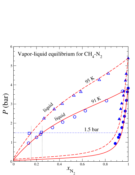
Figure 1.— Comparison between experimental data for the binary system N₂–CH₄ and our PC-SAFT based model (Cordier et al., 2017), for two temperatures: $91$ K (circles) and $95$ K (triangles). Laboratory measurements, already used by Tan et al. (2013), come from various sources: Sprow & Prausnitz (1966) for $91$ K and Parrish & Hiza (1974) for $95$ K (triangles). Squares represent N₂ dissolution data from recent work (Malaska et al., 2017a), respectively, at $89\pm 0.5$ K and $95\pm 0.5$ K. The pressure $P=1.5$ bar represents the value determined by Huygens at ground level.

The physical meaning of terms in Eq. (2) are the following: (A) represents the energy stored in the surface of the bubble, while (B) accounts for the work done by the liquid during the bubble inflation. It can be shown (Brennen, 1995) that the probability of formation of a microbubble of radius $r_{\rm c}$ is proportional to $\exp-W/k_{\rm B}T$, with $k_{\rm B}$ the Boltzmann constant. This consideration clearly favors the above mentioned embryonic ($r_{\rm c}\simeq 10^{-7}$ m) bubbles of pure nitrogen ($x_{\rm N_{2}}\simeq 1$), since these small bubbles have a probability of formation much larger than that of bigger bubbles. The theory also provides the homogeneous nucleation rate $J_{\rm nuc}^{\rm hom}$ (m^-3 s^-1), i.e. the mean number of bubbles reaching the critical radius, per unit of volume of liquid, per unit of time (Brennen, 1995)

$$J_{\rm nuc}^{\rm hom}=N^{*}_{\rm N_{2}}\,\left(\frac{2\sigma}{\pi m_{\rm N_{2}}}\right)^{1/2}\exp-\frac{W}{k_{\rm B}T}$$ (3)

where $N^{*}_{\rm N_{2}}$ (m^-3) is the number of nitrogen molecules, per unit of volume, in the liquid phase, and $m_{\rm N_{2}}$ (kg) represents the mass of a single N₂ molecule. For the mixture under consideration, we found $N^{*}_{\rm N_{2}}\sim 3.4\times 10^{27}$ m^-3, with an extremely low nucleation rate

$$\mathrm{log}_{10}J_{\rm nuc}^{\rm hom}\sim-2\times 10^{5}$$ (4)

For a system like Ligeia Mare, which contains roughly $10^{13}$ m³ of liquid, the time required for the formation of a single bubble is much longer than the age of the universe. These estimations unequivocally rule out homogeneous nucleation, as an efficient bubble formation mechanism, in a Titan’s sea. Neither higher pressures nor the presence of ethane changes this conclusion. At the bottom of a sea, like Ligeia Mare, the pressure is evaluated to be around $3$ bars (Cordier et al., 2017), this higher liquid pressure only decreases the difference $P_{B}-P_{L}$ (in Fig. 1, $1.5$ bar is replaced by $3.0$ bar) and the nucleation rate is not significantly affected. The presence of some amount of ethane, for instance a mole fraction of the order of $0.20$–$0.30$ changes only marginally the values of $N^{*}_{\rm N_{2}}$, while only slightly modifying the surface tension in Eq. (3).

3. Heterogeneous nucleation and bubbles growth

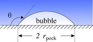
Figure 2.— Heterogeneous nucleation on a flat surface, $r_{\rm pock}$ is the typical maximum dimension of the gas pocket. The contact angle at the liquid-vapor-solid intersection is denoted $\theta$ .

Alternatively to homogeneous nucleation, heterogeneous nucleation may occur in Titan’s seas. It is well known, as a general fact, that heterogeneous nucleation is faster than homogeneous nucleation (Vehkamäki, 2006; Sánchez-Lavega, 2010). The presence of a different interface reduces the height of Gibbs free energy barrier. This is true for all types of phase transition: vapor to liquid, liquid to vapor, liquid to solid, etc. In Titan’s seas, the possible presence of solids may trigger heterogeneous nucleation of nitrogen bubbles. This kind of material could cover the sea bottom, or could be present under the form of suspended particles. The size of a bubble leaving a solid substrate, under the influence of buoyancy forces, can be roughly estimated for a contact angle (see Fig. 2) around $90^{\rm o}$, value which represents the boundary between the low wettability and the high wettability domains. The radius $r_{\rm hetero}$ of the hemispherical vapor nucleus, leaving its solid horizontal substrate, is given by (de Gennes et al., 2004)

$$r_{\rm hetero}\simeq\sqrt{\frac{3\sigma}{\rho g_{\rm Titan}}}$$ (5)

If, for example, we consider a $0.8$:$0.2$ mixture of CH₄ and N₂, a composition that could be typical of the upper layers of liquid, the surface tension should be $\sigma\simeq 10^{-2}$ N m^-1 at $90$ K (see Tab. 1), with a density $\rho\simeq 520$ kg m^-3. These numbers lead to $r_{\rm hetero}\simeq 7\times 10^{-3}$ m, i.e. a diameter of about $\sim 1.4$ cm. If the nucleation occurs at the sea bed, during the rise to the free surface, bubble will undergo an inflation caused by the pressure drop. Using the law of ideal gases and adopting a pressure of $\sim 3$ bars at the sea bottom (Cordier et al., 2017), together with a surface pressure of $1.5$ bar, leads to a radius/diameter enhancement factor of $2^{1/3}\simeq 1.3$, corresponding to bubbles at the surface with a radius of $1.8$ cm. This estimation is more or less comparable to the Cassini RADAR instrument wavelength of $2.2$ cm Other mechanisms, particularly bubbles coalescence, could also contribute to bubble size evolution, they will be discussed in the following. It is striking that the video provided by the NASA press release (Malaska et al., 2017b), associated to the Malaska and co-authors article (Malaska et al., 2017a), show precisely bubbles leaving a solid substrate, which is much larger than bubbles.
Heterogeneous nucleation could also occur on suspended solid particles. To produce cm-sized bubbles, at the moment of solid substrate detachment, requires solids of similar size. However, such relatively large particles could explain, by themselves, the occurrence of “Magic Islands”, without the need for bubbles production, since these preexisting large solids could be good RADAR reflectors (Hofgartner et al., 2016). In addition, while we know plausible formation processes for bubbles, the presence of solids remains entirely speculative. Therefore, the formation of cm-sized bubbles, via a purely heterogeneous process is much more plausible at sea bed than anywhere else. Nonetheless, the existence of suspended sediments, small enough to be undetectable to the RADAR, cannot be ruled out. Solid particles, much smaller than the RADAR wavelength may produce embryonic gas pockets, which could grow during their ascent along a column of liquid. Two distinct growth mechanisms could be at work in such a situation: growth by nitrogen diffusion through bubble surface or the coalescence of bubbles due to stochastic encounters, within their rising stream. The first possibility requires a liquid supersaturated in dissolved nitrogen over the entire column, while the second needs a population of bubbles showing a number of bubbles per unit of volume high enough. We study these two alternative scenarii in the following paragraphs.

3.1. Bubble Growth by Diffusion

Let us imagine, as suggested by Malaska and co-authors (Malaska et al., 2017a), a scenario, according to which a methane-nitrogen Titan’s lake is quickly heated from $\sim 90$ K to $95$ K, i.e. fast enough to avoid any degassing. This operation should leave a liquid supersaturated in N₂. In such a situation, from data plotted in Fig. 1, we conclude that the mole fraction in N₂ should be around $0.25$ instead of $0.15$, just before the evaporation starts. These mole fractions are respectively equivalent to $7\times 10^{3}$ mol m^-3 and $4.2\times 10^{3}$ mol m^-3, leading to a strong supersaturation of $\Delta c_{\rm N_{2}}=2.8\times 10^{3}$ mol m^-3. If homogeneous nucleation appears very unlikely, small sediment particles may generates gas bubbles similar in size to these solid heterogeneities. We have developed a model, that provides the bubbles evolution during their rise, through layers of liquid hydrocarbons supersaturated in nitrogen. This model, based on the well accepted theory of bubbles (Clift et al., 1978), takes into account the bubbles expansion due to pressure drop together with their growth produced by the diffusion of N₂ from the supersaturated liquid to the bubble interior. The details of the model are described in the Appendix. Our simulations have shown strikingly that the final bubble radius $R_{s}$, i.e. obtained at the surface of the sea, does not depend on the initial bubble radius $R_{0}$, but only on the depth $H_{0}$ at which the embryonic bubble is assumed to start its rise. This property is explained by the dependence of rising velocity $U_{b}$ on bubble radius: $U_{b}\propto\sqrt{r_{b}}$. Under this circumstances, smaller bubbles are the slowest; then, they have more time to let diffusion feeding their interior in nitrogen. Numerically, we found that a depth of $H_{0}\sim 0.5$ m is a minimum to get a radius of $R_{s}\sim 1.1$ cm at the surface. The rise along such a relatively small height requires only $\tau_{\rm rise}\sim 9$ s. It is clear that, if tiny sediment particles have a volumic number density high enough, the considered layers of liquid would reach, in a few seconds, the thermodynamic equilibrium with the atmosphere. Therefore, we have to compare $\tau_{\rm rise}$ with the thermal relaxation time $\tau_{\rm therm}$ of such layers. In the literature (Cordier et al., 2012) we found that $\tau_{\rm therm}$ should be of the order of $2$ Titan’s days for $H_{0}=1$ m. Since $\tau_{\rm therm}\propto H_{0}^{2}$, a depth of $H_{0}=0.5$ m leads to $\tau_{\rm therm}\sim 10^{6}$ s. These numbers suggest that nitrogen exsolution, by bubbles transport to the surface, should be much faster than thermal relaxation. In such a case, any modest temperature increase, at the sea surface, would produce an immediate release of nitrogen, under the form of tiny bubbles. As a consequence, liquid layers closest to the atmosphere would quickly lose their supersaturation. This way, embryonic bubbles, produced in deeper layers, would rise through non supersaturated zones, a thermodynamic state which inhibits growth by diffusion. Finally, even if tiny sediment particles are numerous enough to trigger a quantitative nitrogen dissolution, under the form of small bubbles, the mechanism of growth to RADAR visible bubbles, should be rapidly blocked by “de-supersaturation” of top liquid layers. Of course, larger values for $H_{0}$ make the situation worse.
A similar desaturation would occur in the case of cosmic rays reaching the surface, even though Titan’s dense atmosphere is heavily shielded and the overall cosmic ray flux is low (Molina-Cuberos et al., 1999). Let us now consider the growth by bubbles coalescence.

3.2. Bubble Growth by Coalescence

Until this point, we have neglected all possible interaction between bubbles. The features of observed “Magic Islands” suggest the existence of plumes containing a rather large volume density of bubbles. Within a dense population, the probability of the encounters becomes appreciable. When two bubbles collide, they may coalesce, forming a bigger bubble. This effect substantially enhances the diameter of bubbles reaching the surface, after having undergone one or several coalescence during the rise. The simplest effect, producing bubbles collisions, origins in the difference in rise velocities of bubbles of different sizes. The subsequent buoyancy-driven collision rates $\theta_{ij}^{\rm B}$ (m^-3 s^-1) is given by the literature (Prince & Blanch, 1990; Friedlander, 2000)

$$\theta_{ij}^{\rm B}=n_{i}n_{j}S_{ij}(U_{b,i}-U_{b,j})$$ (6)

where $n_{i}$ and $n_{j}$ (m^-3) are the concentration of bubbles of radius $r_{b,i}$ and $r_{b,j}$ (m), and $S_{ij}=\pi(r_{b,i}+r_{b,j})^{2}/4$ (m²). Here $U_{b,k}$ is the rise velocity of the particle $k$. During its ascent, a given bubble $i$ reaches quickly its terminal velocity $U_{b,i}=2\sqrt{g_{\rm Titan}r_{b,i}}/3$ (m s^-1) (Clift et al., 1978). By moving through the liquid, bubbles generate their own, small scale, turbulence, and this expression of $U_{b,i}$ (also used in the model described in the Appendix) implicitly assumes a turbulent close neighborhood. However, as a first approach, we consider this velocity as an average value and we will take typical radius values in order to get the velocity difference term in Eq. (6), non equal to zero. We have gathered in Tab. 2 estimations of rising velocities and rising timescale $\tau_{100}$ for a $100$ m deep sea, using those radius typical values, i.e. $10^{-4}$, $10^{-3}$ and $10^{-2}$ m. Since the goal is getting a final bubble with a radius larger than $1$ cm, and since big bubbles rise faster than small ones (see Tab. 2). faster than small ones, we consider a typical example of a “test bubble” of $1$ mm, riding through a population of $0.1$ mm in radius bubbles. If the differential $\mathrm{d}h$ is the elementary depth variation for our “$1$-mm bubble” during the duration $\mathrm{d}t$, the average number of coalescence events undergone by our “$1$-mm test bubble” is

Table 2Rising terminal velocities $U_{b,i}$ for three radius values. The Titan’s gravity is $g=1.352$ m s^-2, the rising time $\tau_{100}$ is computed for an initial depth of $H_{0}=100$ m.

Bubble radius $r_{bi}$ (m)	$10^{-4}$	$10^{-3}$	$10^{-2}$
$U_{b,i}$ (m s-1)	$7.8\times 10^{-3}$	$2.5\times 10^{-2}$	$7.8\times 10^{-2}$
$\tau_{100}$ (s)	$1.3\times 10^{4}$	$4.1\times 10^{3}$	$1.3\times 10^{3}$

$$\mathrm{d}^{2}N_{c}=\theta^{\rm B}_{ij}\mathrm{d}t\,\mathrm{d}h\,s$$ (7)

where $s$ represents the cross section of the considered column of liquid, we took $s=1$ m² for convenience. By integrating Eq. (7) over time and depth, with $\theta^{\rm B}_{ij}$ assumed approximately constant over the entire column, we get

$$N_{c}\simeq\theta^{\rm B}_{ij}\tau_{100}\,sH_{0}$$ (8)

If coalescence is the only mechanism at work, a simple calculation, based on the conservation of the total quantity of gas contained in bubbles, shows that $N_{c}\sim 10^{6}$ bubbles, with a radius of $0.1$ mm, are needed to make one final $1$ cm in radius bubble. This result can be used to estimate the required order of magnitude of $\theta^{\rm B}_{ij}$, thanks to Eq. (8), we found $\theta^{\rm B}_{ij}\sim 1$ coalescences m^-3 s^-1, over the column of $H_{0}=100$ m. For one single $1$-mm sized bubble (i.e. $n_{i}=1$) rising along the column, we can evaluate the required number density of $0.1$-mm bubbles, needed to get a final centimeter sized bubbles. For that purpose, Eq. (6) is used, together with values available in Tab. 2, to finally obtain $n_{j}\sim 10^{8}$ bubbles per m³ along the entire column (with $r_{b,j}\sim 10^{-4}$ m). Polydisperse bubbles populations may be simply generated by sea floor composition heterogeneities, or caused by stochastic fluctuations in bubble/substrate uncoupling. Clearly, buoyancy-driven bubbles coalescence appears to be an efficient mechanism which could produce cm-sized bubbles in bubbles trajectory ends, within the sea top-layers.

This concentration represents $100$ bubbles per cm³, i.e. a total volume of gas of $4.2\times 10^{-4}$ cm³, per cm³ of liquid. Number which appears reasonable, since it corresponds only to a small fraction of the volume of liquid. In this scenario, bubbles are formed at the sea bed, with a non-uniform distribution in size. The first bundles of bubbles, leaving the depths of the sea, settle all the sea levels. The following generations of bubbles pass through this bubbly medium. As big bubbles are faster than small ones, similarly to our example, big bubbles (e.g. with $r_{b,i}\sim 10^{-3}$ m) aggregate small ones (e.g. with $r_{bi}\sim 10^{-4}$ m).

Collisions induced only by different rising velocities assume a gentle turbulent field, mainly localized in the immediate vicinity of bubbles. In massive bubbles streams, a strong turbulent field may appear. Under such regime, the turbulent collision rate $\theta^{T}_{ij}$ (see Eq. 9) no longer depends on differences of individual velocities. Instead, it can be estimated with (Prince & Blanch, 1990)

$$\theta_{ij}^{\rm T}=0.089\pi n_{i}n_{j}(d_{bi}+d_{bj})^{2}\epsilon^{1/3}(d_{bi}^{2/3}+d_{bj}^{2/3})^{1/2}$$ (9)

where $d_{b}$ is the bubble diameter and $\epsilon$ is the energy dissipation per unit of mass and unit of time (J kg^-1 s^-1). Compared to buoyancy-driven collision, in that case, even bubbles of the same size can coalesce. The factor $\epsilon$ can be estimated using $k_{d}=\epsilon^{1/4}/2\nu^{3/4}$ where $k_{d}$ (m^-1) is the wave number of turbulent eddies and $\nu$ is the liquid kinetic viscosity (Batchelor, 1953). Eddies most affecting bubbles have wave numbers roughly similar to $1/r_{b}$. Density and viscosity of liquid methane, together with an assumed radius of $10^{-3}$ m, yields to $\epsilon\sim 0.4$ J kg^-1 s^-1. Assuming a population of mm sized bubbles, basic computations show that we need a number of $N_{c}=10^{3}$ of such bubbles to build up a cm size final bubble by successive coalescences. For a sea depth of $H_{0}=100$ m, corresponding to $\tau_{100}\sim 10^{3}$ s for a mm size particle, we found the required turbulent collision rate to be of the order of $\theta_{ij}^{\rm T}\sim 10^{-2}$ m^-3 s^-1. We, then, can derive the minimum bubbles density $n_{j}\sim 10^{5}$ m^-3. This represents one single mm size bubble for $10$ cm³, which is a pretty modest concentration. Here, the volume of gas is also, incidentally, equal to $4.2\times 10^{-4}$ cm³ per cm³ of liquid.

As we can see, both coalescence mechanisms, are able to produce bubbles big enough to be detectable at Ligeia Mare surface. This conclusion is true if the number of bubbles initially produced is sufficiently large and if their start their journey to the surface from a depth of the order of $\sim 100$ m. These two coalescence processes may be at work in nature, depending on the size distribution and volumic density by number of bubble populations, initially nucleated at the seabed. We emphasize that turbulence-driven collision rate could dominate if gases are injected in the liquid through hypothetical sea bottom vents. In that case, high $\epsilon$ values could be reached, causing large collision rate. Finally, we stress that break-up radius (Clift et al., 1978; Cordier et al., 2017) $r_{\rm bk}\simeq 4\sqrt{\sigma/(\rho\,g)}$ cannot be overcome by any mechanism. This remains an absolute upper limit, of the order of $\sim 2.3$ cm ($\sim 4.6$ cm in diameter) (Cordier et al., 2017), for bubble size.

4. Bubbles RADAR Signature

Throughout the discussion, the criterion used to decide whether or not bubbles could be RADAR detectable is based on their size. Objects possessing a diameter comparable to the wavelength (i.e. $2.16$ cm) have been considered to have a measurable effect. This approach is relevant in first approximation, but it is not—by essence—not quantitative, and it neglects effects like multiple scattering, which may be important in the context. Previous works (Hofgartner et al., 2016) have estimated the possible single scattering albedo of a population of relatively small bubbles ($r_{b}\sim 10^{-3}$ m), i.e. using the Rayleigh scattering theory (Bohren & Huffman, 2014). For larger reflectors, i.e. with sizes comparable to the wavelength, the Mie scattering theory is required (Mie, 1908).

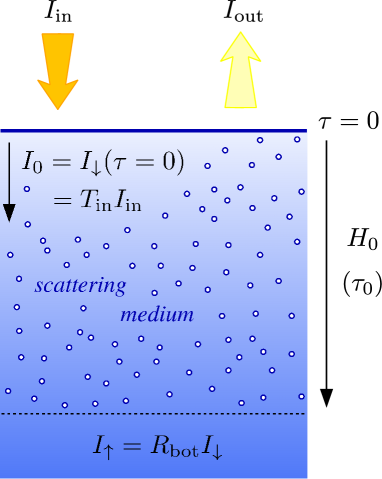
Figure 3.— Sketch of the liquid column containing bubbles. $I_{\rm in}$ is the incident RADAR photons flux, while $I_{\rm out}$ is the signal returning back to the emitter. The total height of the column is denoted $H_{0}$ corresponding to the optical depth $\tau_{0}$. The bottom of the column, filled by bubbles, does not necessarily correspond to the sea bed.

We then built a model in which a column of liquid is filled by bubbles, with a total height denoted $H_{0}$, corresponding to the “optical” depth $\tau_{0}$ (see Fig. 3). The geometry is simplified: the flux of energy $I_{\rm in}$ coming from the spacecraft arrives at the sea-atmosphere interface with a normal incidence. This approximation is perfectly relevant in our case, since during T92 and T104 observations, the incident angles were respectively $6.^{\rm o}0$ and $11.^{\rm o}5$ (Hofgartner et al., 2016). The effects of the polarization, and the absorption, are neglected as suggested by previous works (Hofgartner et al., 2016). In that frame, using a two-stream radiative transfer model (Bohren & Huffman, 2014), accounting for multiscattering by principle, the energy fluxes, through the liquid, in downward and upward direction are, respectively,

$$I_{\downarrow}=D+C(1-\tau^{*})$$ (10)

$$I_{\uparrow}=D-C(1+\tau^{*})$$ (11)

where $\tau^{*}$ is the optical depth corrected by the asymmetry factor $g_{b}$ of bubbles: $\tau^{*}=(1-g_{b})\tau$. The asymmetry factor is computed in the frame of the Mie’s theory. The coefficients $D$ and $C$ are given as a functions of $I_{0}=I_{\downarrow,\tau=0}$, and $\tau^{*}_{0}$ the total optical depth of the column (see Fig. 3), we have

$$C=\frac{(1-R_{\rm bot})I_{0}}{2+(1-R_{\rm bot})\tau^{*}_{0}}$$ (12)

$$D=\frac{2+(1-R_{\rm bot})(\tau^{*}_{0}-1)}{2+(1-R_{\rm bot})\tau^{*}_{0}}I_{0}$$ (13)

where $R_{\rm bot}$ represents the reflectance at the bottom of the column, or equivalently at the sea floor. The uncorrected total optical depth $\tau_{0}$, of the column of the liquid, is provided by

$$\tau_{0}=\int_{0}^{H_{0}}\beta\,\mathrm{d}z$$ (14)

in which $1/\beta$ represents the radar photon’s mean-free path; $\beta$ is a function of the number density $n_{b}$ (bubbles m^-3) and of the bubbles Mie’s cross section $\sigma_{\rm Mie}$: $\beta=n_{b}\,\sigma_{\rm Mie}$. The flux leaving the sea and returning to the RADAR is $I_{\rm out}=(1-R_{\rm in})I_{\uparrow,\tau=0}$, here, the reflectance $R_{\rm in}$ of the interface sea atmosphere, is assumed to take into account the effect of the rugosity (Grima et al., 2017), which is usually, except in the occurrence of a “Magic Island” event, measured to be very small (Wye et al., 2009; Zebker et al., 2014; Grima et al., 2017; Stephan et al., 2010; Barnes et al., 2011).
In order to quantify the RADAR signature of bubbles, we compare the reflected flux with and without the presence of bubbles. For that purpose, we introduce the quantity $R_{\rm bubb}=I_{\rm out}/I_{\rm in}$ which has to be compared to the “ clear sea,” i.e. without bubbles, global reflectance given by $R_{\rm cs}=R_{\rm bot}T_{\rm in}^{2}+R_{\rm in}$, where $T_{\rm in}=1-R_{\rm in}$. For that purpose, we denote Bubbles Radar Signal Amplification (BRSA) as the ratio $R_{\rm bubb}/R_{\rm cs}$.

As a first approach, we have chosen to neglect the upward flux of RADAR photons at the bottom of the column: $I_{\uparrow}(\tau_{0})=0$. Below the bubbly column, the microwave photons are considered to be lost. In other words, the reflectance at the bottom of the column is taken equal to zero: $R_{\rm bot}=0$. Taking the methane permittivity (Mitchell et al., 2015) $\epsilon_{r}({\rm\tiny CH_{4}})=1.72$ as a reference, we have explored the influences of the bubble radius $r_{b}$, of the number of bubbles per unit of volume $n_{b}$ and of the column height $H_{0}$, results are gathered in Fig. 4. Not surprisingly, large bubble radii favor a strong backscattering (Fig. 4 a). Similar effects are found for the influence of the number of bubbles per unit of volume $n_{b}$ (Fig. 4 b) and the total height $H_{0}$ of the bubbly column (Fig. 4 c).

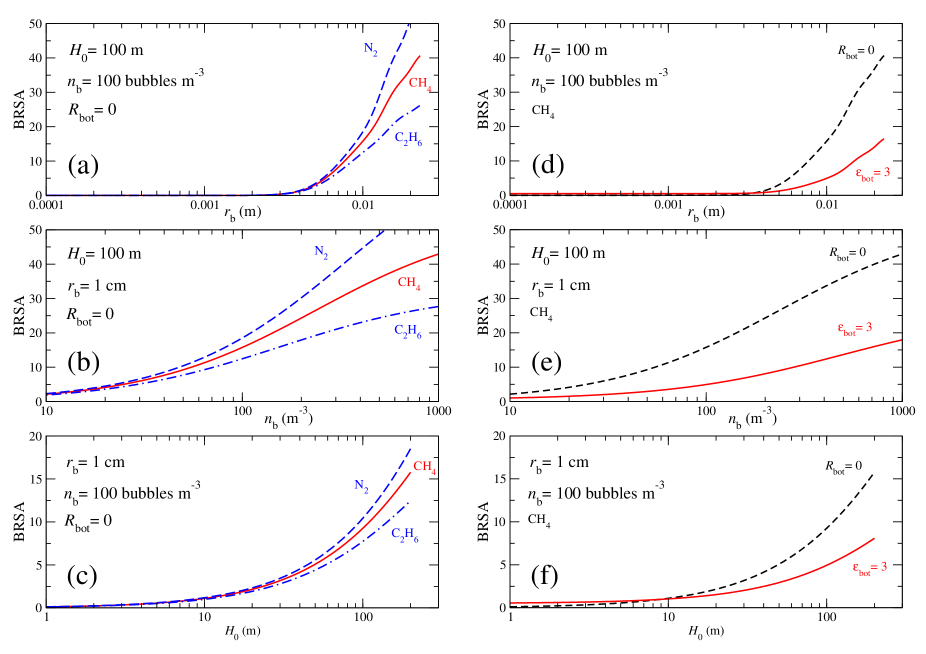
Figure 4.— Influence of bubble stream parameters on RADAR Signal Amplification (BRSA). (a) Influence bubble radius $r_{b}$, the simulation is stopped at the bubbles break-up radius $r_{\rm breakup}\sim 2.3$ cm (Cordier et al., 2017). While the solid red curve has been computed using the methane permittivity $\epsilon_{r}=1.72$ (Mitchell et al., 2015), dashed and dotted-dashed blue lines correspond, respectively, to liquid nitrogen ($\epsilon_{r}=1.55$; Hosking et al., 1993) and ethane ($\epsilon_{r}=2.00$; Mitchell et al., 2015). (b) Influence of volume density $n_{b}$ of bubbles. (c) Influence of the total height of the column $H_{0}$ (see Fig. 3), the considered range of $H_{0}$ has been limited to $0-200$ m, since the bathymetry of Ligeia Mare shows a maximum depth around $200$ m (Hayes, 2016). In panels (d), (e) and (f), we report computations including a non-zero reflectance of the sea floor; its permittivity is $\epsilon_{\rm bot}=3$, which is probably a very high value (corresponding to $R_{\rm bot}\simeq 2$%. In these panels, the methane $R_{\rm bot}=0$ curve is recalled for comparison.

The dielectric permittivity of the liquid also has its influence. Taking the permittivity of pure liquid nitrogen: $\epsilon_{r}({\rm N_{2}})=1.55$ (Hosking et al., 1993), we found a BRSA higher than values obtained with CH₄ permittivity (see Fig. 4, panels (a), (b), (c)). In contrast, a simulation with liquid ethane permittivity, $\epsilon_{r}({\rm C_{2}H_{6}})=2.00$ (Mitchell et al., 2015), yields to a reduction of the BRSA. Perhaps surprisingly, a low liquid permittivity favors the bubble stream RADAR reflection. The chemical composition of Titan is still not firmly known, but we emphasize that, accidentally, the mean value of nitrogen and ethane respective permittivities is very close to the methane individual value. Consequently, a sea with a composition in N${}_{2}:$CH${}_{4}:$C₂H₆ around $0.20:0.40:0.20$ will show a permittivity close to the pure liquid methane value $\epsilon_{r}({\rm CH_{4}})=1.72$ (Mitchell et al., 2015). In Ref. Hofgartner et al. (2016), the Normalized Radar Cross Section (NRCS) along the flyby tracks is reported in Figures 4 and 5. In these figures, the NRCS “peaks” corresponding to T92 and T104 transient feature events offer the opportunity to estimate the ratio of the quantity of radar photons backscattered with a the presence of a “Magic Island” and without such a structure. The height of NRCS “peaks,” measured to be between $\sim 6$ and $\sim 9.5$ in dB, leads to ratios ranging between $\sim 6$ and $\sim 10$. This means that radar reflectors present at Ligeia Mare, during “Magic Island” episodes, enhance the local reflectivity by a factor in the interval $6-10$. Panel (c) in Fig. 6 of the same reference, gives another opportunity to evaluate the “reflectivity enhancement” during Ligeia Mare overbrightness events. A quick comparison of NRCS predicted by the sea floor model plotted in this figure and actual measurements performed during T92 and T104, leads to energy ratios magnified by a factor of $\sim 10-16$. If we keep a factor around $\sim 10$, which corresponds to what we call BRSA, the Ligeia Mare “Magic Islands” can be easily explained by a column of $H_{0}\sim 100$ m, containing around $100$ centimetric bubbles per cubic meters, this, if sea floor reflectance can be neglected.
Unfortunately, the hypothesis of the seabed zero-reflectivity is an oversimplification. Actually, the sea floor partly re-emits the incident RADAR beam energy. This property has been utilized to derived Ligeia Mare bathymetry (Hayes, 2016). For that purpose, two distinct echoes in altimetry tracks (Hayes, 2016) have been detected (Hayes, 2016), one caused by the surface and the second produced by energy backscattered by the sea bottom. Thus, we have compared published values of NRCS (Hayes, 2016) of these echoes; we found a difference in dB around $30$, which leads to a ratio in energy of about $\sim 10^{3}$. The flux coming from the deepest part of the sea is obviously the weakest, suggesting a quite low reflectance of the sea bottom. Using RADAR observation, and their models, Hofgartner and co-authors (Hofgartner et al., 2016) propose a sea floor dielectric constant around $\epsilon_{r,{\rm seafloor}}=1.99$, but the actual value is not well constrained since the real nature of the seabed is not known. Titan belongs to the so-called “icy moons;” therefore, water ice is recognized to be a major component of Titan’s geological layers (Baland et al., 2014). If we assume a sea floor composed by pure water ice, its microwaves permittivity should be around $\epsilon_{r,{\rm ice}}=3$ (Bradford et al., 2009). The actual value depends on the porosity of the ice and on the nature of the material mixed within it. Adopting $\epsilon_{r,{\rm ice}}=3$ for the seabed, which has to be understood as a high value (Le Gall et al., 2016), we computed the corresponding BRSAs. They are compared to their counterparts computed with a bottom zero-reflectivity; results are plotted in panels (d), (e), and (f) of Fig. 4. These simulations demonstrate that a non-zero bottom reflectivity ($R_{\rm bot}\neq 0$) damps the BRSAs, i.e. the ratios $R_{\rm bubb}/R_{\rm cs}$. This behavior is caused by the addition of the term $R_{\rm bot}T^{2}_{\rm in}$ in the expression of $R_{\rm cs}$.

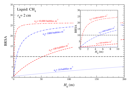
Figure 5.— The Bubbles Radar Signal Amplification (BRSA) for a column of liquid methane, harboring bubbles with a radius of $2$ cm, as a function of the total height $H_{0}$ of the column. Several volume densities of bubbles are considered: $n_{b}=10$, $100$, $1000$, and $10{,}000$ bubbles m^-3. The explanation of Ligeia Mare “Magic Island” requires BRSA$\sim 10$. The panel inserted on the right-hand side is a magnification of the main figure in the region of the origin.

Nonetheless, as we can see in Fig. 4, even with a relatively large value for $R_{\rm bot}$ ($\epsilon_{r,{\rm seafloor}}=3$ corresponds to $R_{\rm bot}\sim 2$%), reasonable combinations of $r_{b}$, $n_{b}$ and $H_{0}$ can be found, with a resulting BRSA around $\sim 10$, a value that explains the observed Ligeia Mare “Magic Island.” For instance, a column of $H_{0}=100$ m, containing $n_{b}=100$ bubbles m^-3 with $r_{b}=2$ cm has a BRSA of $\sim 14$. If we adopt a bubble radius close to the maximum value allowed by bubble physics, i.e. $r_{b}=2$ cm which is approximately the break-up radius, we can search for the minimum height $H_{0}$ required to get a BRSA around $\sim 10$. This is done in Fig. 5, in which several values for $n_{b}$ are assumed. Since with $r_{b}=2$ cm, one cannot include more than $\sim 10,000$ bubbles within one cubic meter, $n_{b}=10{,}000$ bubbles m^-3 represents a geometrical maximum. As we can see, even with $r_{b}=2$ cm and $n_{b}=10{,}000$ bubbles m^-3, we need $H_{0}\sim 0.5$ m to reach BRSA$\sim 10$. According to the discussion conducted in Sect. 3.1, it appears impossible to form centimetric bubbles due to an heating starting at the sea surface. One more time, a scenario based on a bubbles production in the depth of Ligeia Mare looks more plausible than a pure surface phenomenon. Indeed, Fig. 5 tells us that a few tens of meters, with a relatively modest number of bubbles per cubic meters, produced the required value for the Bubbles Radar Signal Amplification.

5. Conclusion

In this work, we have demonstrated that the homogeneous nucleation of small bubbles of N₂ is impossible under the conditions of the Titan surface. Heterogeneous nucleation, i.e. involving a solid substrate, is much more easier. Such substrates could be found at the seabed or under the form of small sediment particles suspended in the liquid. However, in that case, a growth mechanism has to be at work to obtain bubbles large enough to be efficient RADAR reflectors. While the growth by diffusion in nitrogen supersaturated layers appears to be very difficult, if not impossible; the growth by coalescence, along a bubbly column has been found to be a powerful process to get large bubbles. In this case, such a column must have a height that is more or less comparable to Ligeia Mare depth. We also developed a model of reflection of the RADAR wave by a stream of bubbles in a Titan’s sea. This approach also favors streams of bubbles with a vertical extension of several tens of meters.
In short, to explain the “Magic Islands,” one scenario, based on bubbles, has the best plausibility if it implies that bubbles are released or formed in the depths of the sea.

Appendix A Model of Bubble Ascension and Growth

In a column of liquid, the gas bubbles have a vertical upward motion due to buoyancy forces, the liquid flowing around bubbles rapidly reaches a high Reynolds number. In such a situation, the bubble velocity $U_{b}$ (m s^-1) can be estimated with (Clift et al., 1978)

$$U_{b}=\frac{2}{3}\sqrt{\frac{ga\Delta\rho}{\rho}}$$ (A1)

since, during their ascent to the free surface, the bubbles distort, the parameter $a$ represents a characteristic length of bubble geometry. For the sake of simplicity, we adopted the approximation $a\simeq r_{b}$, with $r_{b}$ the bubble “radius” or typical size. In addition, we have $\Delta\rho=\rho_{\rm liq}-\rho_{\rm gas}\simeq\rho_{\rm liq}$, then $\Delta\rho/\rho\sim 1$, leading to

$$U_{b}\simeq\frac{2}{3}\sqrt{g_{\rm Titan}r_{b}}$$ (A2)

We emphasize that, before adopting the velocity given by Eq. (A1), we performed tests using the so-called “Levich velocity”

$$U\simeq\frac{\rho\,g_{\rm Titan}\,r_{b}^{2}}{9\eta_{\rm liq}}$$ (A3)

where $\eta_{\rm liq}$ is the viscosity of the liquid, for which velocity is valid for relatively moderate Reynolds numbers, i.e. $50\lesssim Re\lesssim 200$ (Clift et al., 1978). In that case, the Reynolds numbers, obtained in our simulation, quickly reached $\sim 10^{3}$, to finally increase to $\sim 10^{5}$ near the surface, far beyond the validity of Eq. (A3). We, then, turned to Eq. (A1) to get more consistent numerical simulations. The initial depth of $H_{0}\sim 0.50$ m, found to get centimeter-sized bubbles at the surface, has to be understood as a minimum. Indeed, in the early times of the ascent, the Reynolds numbers were below $\sim 200$ and Levich’s form should have been employed during this stage, leading to larger $H_{0}$’s values.
In the case of the fluid sphere, for high Reynolds numbers, the Sherwood number and the Peclet number are linked through the equation (Clift et al., 1978)

$$\mathrm{Sh}=\frac{2}{\sqrt{\pi}}\mathrm{Pe}^{1/2}$$ (A4)

We recall that

$$\mathrm{Sh}=\frac{kl}{D}$$ (A5)

where $k$ is the convective mass transfer rate (m s^-1), $l$ is a characteristic length (m), and $D$ is the molecular diffusion coefficient (m² s^-1), in our context $D\sim D_{\rm N_{2}-CH_{4}}$. The Peclet number is given by

$$\mathrm{Pe}=\frac{Ul}{D}$$ (A6)

Using the above equation and taking $l\sim r_{b}$, we can express that the convective mass transfer rate are linked through the equation (Clift et al., 1978)

$$k=\sqrt{\frac{2}{\pi}}\sqrt{\frac{D_{\rm N_{2}-CH_{4}}U_{b}}{r_{b}}}$$ (A7)

Here, the N₂ bubble content, noted as $n$ (mol) is driven by the equation

$$\frac{\mathrm{d}n}{\mathrm{d}t}=k\,4\pi r_{b}^{2}\,\Delta c_{\rm N_{2}}$$ (A8)

This equation can be easily reformulated as

$$\frac{\mathrm{d}n}{\mathrm{d}h}=-\sqrt{\frac{2}{\pi}}\left(\frac{D_{\rm N_{2}-CH_{4}}}{r_{b}U_{b}}\right)^{1/2}4\pi r_{b}^{2}\,\Delta c_{\rm N_{2}}$$ (A9)

where $h$ (m) is the depth at which the bubble is located at a particular moment. For convenience, we have considered time as a function of $h$, which has been chosen as our independent variable. Thus, $t(h)$ follows the law

$$\frac{\mathrm{d}t}{\mathrm{d}h}=-\frac{1}{U_{b}}$$ (A10)

The external bubble pressure $P_{e}$ is ruled by the hydrostatic law $P_{e}(h)=P_{0}+\rho g_{\rm Titan}h$ where $P_{0}$ represents the atmospheric pressure at the sea surface, leading to

$$\frac{\mathrm{d}P_{e}}{\mathrm{d}h}=\rho g_{\rm Titan}$$ (A11)

With $P_{i}$ as the internal pressure of bubbles, assumed spherical, we can write the ideal gas law

$$P_{i}(h)\times\frac{4}{3}\pi r_{b}^{3}=n(h)R_{\rm gas}T$$ (A12)

with $R_{\rm gas}$ as the gas constant. The pressures $P_{e}$ and $P_{i}$ are linked by Laplace’s equation

$$P_{i}=P_{e}+\frac{2\sigma}{r_{b}}$$ (A13)

from this, we can easily derive the equation governing the evolution of the bubble radius

$$\frac{\mathrm{d}r_{b}}{\mathrm{d}h}=-\frac{R_{\rm gas}T}{P_{i}}\sqrt{\frac{2}{\pi}}\left(\frac{D_{\rm N_{2}-CH_{4}}}{r_{b}U_{b}}\right)^{1/2}\Delta c_{\rm N_{2}}-\frac{\rho g_{\rm Titan}r_{b}}{3P_{i}}$$ (A14)

In summary, we have four unknowns: $n(h)$, $t(h)$, $P_{e}(h)$, and $r_{b}(h)$, which are found by numerically integrating (Nougier, 1987) the system of four equations: (A9)–(A11) and (A14). Assuming an isothermal column of liquid, at temperature $T$, showing a uniform supersaturation $\Delta c_{\rm N_{2}}$ in dissolved N₂, these equations are solved adopting a starting depth $H_{0}$ and an initial radius $R_{0}$ for bubbles.

Appendix B Diffusion coefficient of nitrogen in liquid methane

The N₂ molecules, initially in the vicinity of a given microbubble, can migrate toward the bubble interior under the influence of thermal agitation. The literature proposes several methods to estimate the diffusion coefficient $D_{\rm N_{2}-CH_{4}}$ of the nitrogen molecule through liquid methane (Poling et al., 2007). Among these methods, the Wilke–Chang technique (Wilke & Chang, 1955) is widely used. It is based on correlations and provides diffusion coefficient $D^{0}_{\rm A-B}$ of a compound A in a compound B, at infinite dissolution, i.e. when the mole fraction of A is very small. For our system, one can write

$$D^{0}_{\rm N_{2}-CH_{4}}=\frac{7.4\times 10^{-11}(\Phi M_{\rm CH_{4}})^{1/2}T}{\eta_{\rm CH_{4}}V_{\rm N_{2}}^{0.6}}$$ (B1)

with $D^{0}_{\rm N_{2}-CH_{4}}$ in cm² s^-1, $\Phi$ is an adimensional coefficient around unity, $M_{\rm CH_{4}}$ is the molecular weight (g mol^-1) of methane, $\eta_{\rm CH_{4}}$ is the dynamic viscosity of liquid methane (Pa s), and $V_{\rm N_{2}}$ is the molar volume of solute N₂ at its normal boiling temperature (cm³ mol^-1). The molecular weight has the well known value $M_{\rm CH_{4}}=16.04$ g mol^-1, the viscosity is provided by the literature (Hellemans et al., 1970) $\eta_{\rm CH_{4}}\simeq 1.7\times 10^{-3}$ Pa s and the molar volume $V_{\rm N_{2}}=35$ cm³ mol^-1 (Lide, 1974). At $T=95$ K, these numbers lead to $D^{0}_{\rm N_{2}-CH_{4}}\simeq 2\times 10^{-6}$ cm² s^-1. This determination is comparable to those published for other simple molecules in the liquid state (Poling et al., 2007).
Liquid methane, in equilibrium with a vapor dominated by nitrogen, such as in the case of Titan, should contain an amount of dissolved nitrogen around $0.15$ in mole fraction (see Fig. 1). Then the assumption of infinite dissolution is not valid in our context. Fortunately, empirical corrections are available and the diffusion coefficient $D_{\rm AB}$ can be derived from coefficients $D^{0}_{\rm AB}$ and $D^{0}_{\rm BA}$ obtained in the frame of the hypothesis of infinite dissolution. For instance, one may use (Poling et al., 2007)

$$D_{\rm AB}=(D^{0}_{\rm BA}x_{\rm A}+D^{0}_{\rm AB}x_{\rm B})\,\alpha$$ (B2)

where $x_{\rm A(B)}$ are the respective mole fraction and $\alpha$ is a thermodynamic coefficient, which is not too different from the unity. Using an approach similar to the one previously done for nitrogen, we computed an estimation for the diffusion coefficient of methane in liquid nitrogen, in the case of large dissolution, $D^{0}_{\rm CH_{4}-N_{2}}\simeq 4\times 10^{-5}$ cm² s^-1, using $\eta_{\rm N_{2}}\sim 10^{-4}$ Pa s (Forster, 1963). Our final estimation for the diffusion coefficient of N₂ in liquid CH₄ is $D_{\rm N_{2}-CH_{4}}\simeq 10^{-5}$ cm² s^-1.

References

- Baland et al. (2014) Baland, R.-M., Tobie, G., Lefèvre, A., & Van Hoolst, T. 2014, Icarus, 237, 29
- Barnes et al. (2011) Barnes, J. W., Soderblom, J. M., Brown, R. H., et al. 2011, Icarus, 211, 722
- Batchelor (1953) Batchelor, G. K. 1953, The Theory of Homogeneous Turbulence (Cambridge: Cambridge University Press)
- Bohren & Huffman (2014) Bohren, C. F., & Huffman, D. R. 2014, Absorption and Scattering of Light by Small Particles, 2nd edn. (Wiley-VCH)
- Bradford et al. (2009) Bradford, J. H., Harper, J. T., & Brown, J. 2009, Water Resour. Res., 45, W08403
- Brennen (1995) Brennen, C. E. 1995, Cavitation and Bubble Dynamics (Oxford University Press)
- Clift et al. (1978) Clift, R., Grace, J. R., & Weber, M. E. 1978, Bubbles, Drops and particles (New York, San Fransisco, London: Academic Press)
- Cordier et al. (2017) Cordier, D., García-Sánchez, F., Justo-García, D. N., & Liger-Belair, G. 2017, Nat. Astron., 1, 0102
- Cordier et al. (2012) Cordier, D., Mousis, O., Lunine, J. I., et al. 2012, Planet. Space Sci., 61, 99
- de Gennes et al. (2004) de Gennes, P.-G., Brochard-Wyart, F., & Quéré, D. 2004, Capillarity and Wetting Phenomena: Drops, Bubbles, Pearls, Waves (New York: Springer), doi:10.1007/978-0-387-21656-0
- Forster (1963) Forster, S. 1963, Cryogenics, 3, 176
- Friedlander (2000) Friedlander, S. K. 2000, Smoke, Dust and Haze: fundamentals of aerosol dynamics, 2nd edn. (Oxford: Oxford University Press)
- Grima et al. (2017) Grima, C., Mastrogiuseppe, M., Hayes, A. G., et al. 2017, Earth Planet. Sci. Lett., 474, 20
- Hayes (2016) Hayes, A. G. 2016, Annu. Rev. Earth Planet. Sci., 44, 57
- Hellemans et al. (1970) Hellemans, J., Zink, H., & Van Paemel, O. 1970, Physica, 46, 395
- Hofgartner et al. (2014) Hofgartner, J. D., Hayes, A. G., Lunine, J. I., et al. 2014, Nat. Geosci., 7, 493
- Hofgartner et al. (2016) —. 2016, Icarus, 271, 338
- Hosking et al. (1993) Hosking, M. W., Tonkin, B. A., Proykova, Y. G., et al. 1993, Supercond. Sci. Technol., 6, 549
- Le Gall et al. (2016) Le Gall, A., Malaska, M. J., Lorenz, R. D., et al. 2016, J. Geophys. Res., 121, 233
- Leifer et al. (2017) Leifer, I., Chernykh, D., Shakhova, N., & Semiletov, I. 2017, Cryosphere, 11, 1333
- Leifer et al. (2015) Leifer, I., Solomon, E., von Deimling, J. S., et al. 2015, Mar. Pet. Geol., 68, 806
- Lide (1974) Lide, D. P., ed. 1974, CRC Handbook of Chemistry and Physics, 74th edn. (CRC PRESS)
- Malaska et al. (2017a) Malaska, M. J., Hodyss, R., Lunine, J. I., et al. 2017a, Icarus, 289, 94
- Malaska et al. (2017b) —. 2017b, Experiments Show Titan Lakes May Fizz with Nitrogen, https://www.nasa.gov/feature/jpl/experiments-show-titan-lakes-may-fizz-with-nitrogen, [Online; accessed 29-May-2017]
- Mie (1908) Mie, G. 1908, Ann. Phys. (Berl.), 330, 377
- Mitchell et al. (2015) Mitchell, K. L., Barmatz, M. B., Jamieson, C. S., Lorenz, R. D., & Lunine, J. I. 2015, Geophys. Res. Lett., 42, 1340
- Molina-Cuberos et al. (1999) Molina-Cuberos, G. J., López-Moreno, J. J., Rodrigo, R., Lara, L. M., & O’Brien, K. 1999, Planet. Space Sci., 47, 1347
- Nougier (1987) Nougier, J. P. 1987, Méthodes de calcul numérique (Paris: Masson)
- Parrish & Hiza (1974) Parrish, W. R., & Hiza, M. J. 1974, Adv. Cryog. Eng., 19, 300
- Poling et al. (2007) Poling, B. E., Prausnitz, J. M., & O’Connell, J. 2007, The Properties of Gases and Liquids, 5th edn. (Englewood Cliffs: McGraw-Hill Professional)
- Prince & Blanch (1990) Prince, M. J., & Blanch, H. W. 1990, AIChE J., 36, 1485
- Sánchez-Lavega (2010) Sánchez-Lavega, A. 2010, An Introduction to Planetary Atmospheres (CRC Press)
- Sprow & Prausnitz (1966) Sprow, F. B., & Prausnitz, J. M. 1966, AIChE J., 12, 780
- Stephan et al. (2010) Stephan, K., Jaumann, R., Brown, R. H., et al. 2010, Geophys. Res. Lett.
- Stofan et al. (2007) Stofan, E. R., Elachi, C., Lunine, J. I., et al. 2007, Nature, 445, 61
- Tan et al. (2013) Tan, S. P., Kargel, J. S., & Marion, G. M. 2013, Icarus, 222, 53
- Vehkamäki (2006) Vehkamäki, H. 2006, Classical Nucleation Theory in Multicomponent Systems (Berlin, Heidelberg: Springer)
- Volmer & Weber (1926) Volmer, M., & Weber, A. 1926, Zeit. Physik. Chemie, 119, 277
- Wilke & Chang (1955) Wilke, C. R., & Chang, P. 1955, AIChE J., 1, 264
- Wye et al. (2009) Wye, L. C., Zebker, H. A., & Lorenz, R. D. 2009, Geophys. Res. Lett., 36, L16201
- Zebker et al. (2014) Zebker, H., Hayes, A., Janssen, M., et al. 2014, Geophys. Res. Lett., 41, 308
- Zeldovich (1943) Zeldovich, J. B. 1943, Acta Physicochimica, URSS, 18, 1