Orthogonal Point Location and Rectangle Stabbing Queries in 3-d

Abstract

In this work, we present a collection of new results on two fundamental problems in geometric data structures: orthogonal point location and rectangle stabbing.

• Orthogonal point location. We give the first linear-space data structure that supports 3-d point location queries on $n$ disjoint axis-aligned boxes with optimal $O\left(\log n\right)$ query time in the (arithmetic) pointer machine model. This improves the previous $O\left(\log^{3/2}n\right)$ bound of Rahul [SODA 2015]. We similarly obtain the first linear-space data structure in the I/O model with optimal query cost, and also the first linear-space data structure in the word RAM model with sub-logarithmic query time.

• Rectangle stabbing. We give the first linear-space data structure that supports 3-d $4$-sided and $5$-sided rectangle stabbing queries in optimal $O(\log_{w}n+k)$ time in the word RAM model. We similarly obtain the first optimal data structure for the closely related problem of 2-d top-$k$ rectangle stabbing in the word RAM model, and also improved results for 3-d 6-sided rectangle stabbing.

For point location, our solution is simpler than previous methods, and is based on an interesting variant of the van Emde Boas recursion, applied in a round-robin fashion over the dimensions, combined with bit-packing techniques. For rectangle stabbing, our solution is a variant of Alstrup, Brodal, and Rauhe’s grid-based recursive technique (FOCS 2000), combined with a number of new ideas.

1 Introduction

In this work we present a plethora of new results on two fundamental problems in geometric data structures: (a) orthogonal point location (where the input rectangle or boxes are non-overlapping), and (b) rectangle stabbing (where the input rectangles or boxes are overlapping).

1.1 Orthogonal point location

Point location is among the most central problems in the field of computational geometry, which is covered in textbooks and has countless applications. In this paper we study the orthogonal point location problem. Formally, we want to preprocess a set of $n$ disjoint axis-aligned boxes (hyperrectangles) in $\mathbb{R}^{d}$ into a data structure, so that the box in the set containing a given query point (if any) can be reported efficiently. There are two natural versions of this problem, for (a) arbitrary disjoint boxes where the input boxes need not fill the entire space, and (b) a subdivision where the input boxes fill the entire space.

Arbitrary disjoint boxes.

Historically, the point location problem has been studied in the pointer machine model and the main question has been the following:

“Is there a linear-space structure with $O(\log n)$ query time?”

In 2-d this question has been successfully resolved: there exists a linear-space structure with $O(\log n)$ query time [26, 25, 16, 36, 39] (actually this result holds for nonorthogonal point location). In 3-d there has been work on this problem [17, 23, 2, 32], but the question has not yet been resolved. The currently best known result on the pointer machine model is a linear-space structure with $O(\log^{3/2}n)$ query time by Rahul [32]. In this paper,

• we obtain the first linear-space structure with $O(\log n)$ query time for 3-d orthogonal point location for arbitrary disjoint boxes. The structure works in the (arithmetic) pointer machine model and is optimal in this model.

The orthogonal point location problem has been studied in the I/O-model and the word RAM as well (please see Section A in the appendix for a brief description of these models). In the I/O model, an optimal solution is known in 2-d [21, 6]: a linear-space structure with $O(\log_{B}n)$ query time, where $B$ is the block size (this result holds for nonorthogonal point location). However, in 3-d the best known result is a linear-space structure with a query cost of $O(\log_{B}^{2}n)$ I/Os by Nekrich [27] (for orthogonal point location for disjoint boxes).

• In the I/O model, we obtain the first linear-space structure with $O(\log_{B}n)$ query cost for 3-d orthogonal point location for arbitrary disjoint boxes. This result is optimal.

In the word RAM model, an optimal solution in 2-d was given by Chan [10] with a query time of $O\left(\log\log U\right)$, assuming that input coordinates are in $\left[U\right]=\{0,1,\ldots,U-1\}$. However, in 3-d the best known result for arbitrary disjoint boxes is a linear-space structure with $O\left(\log n\log\log n\right)$ query time: this result was not stated explicitly before but can obtained by an interval tree augmented with Chan’s 2-d orthogonal point location structure [10] at each node. Our above new result with logarithmic query time is already an improvement even in the word RAM, but we can do slightly better still:

• In the $w$-bit word RAM model, we obtain the first linear-space structure with sub-logarithmic query time for 3-d orthogonal point location for arbitrary disjoint boxes. The time bound is $O(\log_{w}n)$. (We do not know whether this result is optimal, however.)

Subdivisions.

In the plane, the two versions of the problem are equivalent in the sense that any arbitrary set of $n$ disjoint rectangles can be converted into a subdivision of $\Theta\left(n\right)$ rectangles via the vertical decomposition. In 3-d, the two versions are no longer equivalent,

since there exist sets of $n$ disjoint boxes that need $\Omega\left(n^{3/2}\right)$ boxes to fill the entire space. See figure on the right.

In 3-d the special case of a subdivision is potentially easier than the arbitrary disjoint boxes setting, as the former allows for a fast $O(\log^{2}\log U)$ query time in the word RAM model with $O(n\log\log U)$ space, as shown by de Berg, van Kreveld, and Snoeyink [15] (with an improvement by Chan [10]).

• In the word RAM model, we further improve de Berg, van Kreveld, and Snoeyink’s method to achieve a linear-space structure with $O(\log^{2}\log U)$ query time for 3-d orthogonal point location on subdivisions.

1.2 Rectangle stabbing

Rectangle stabbing is a classical problem in geometric data structures [1, 3, 7, 13, 32], which is as old, and as equally natural, as orthogonal range searching—in fact, it can be viewed as an “inverse” of orthogonal range searching, where the input objects are boxes and query objects are points, instead of vice versa. Formally, we want to preprocess a set $S$ of $n$ axis-aligned boxes (possibly overlapping) in $\mathbb{R}^{d}$ into a data structure, so that the boxes in $S$ containing a given query point $q$ can be reported efficiently. (As one of many possible applications, imagine a dating website, where each lady is interested in gentlemen whose salary is in a range $[S_{1}{,}S_{2}]$ and age is in a range $[A_{1}{,}A_{2}]$; suppose that a gentleman with salary $x_{q}$ and age $y_{q}$ wants to identify all ladies who might be potentially interested in him.)

Throughout this paper, we will assume that the endpoints of the rectangles lie on the grid $[2n]^{3}$ (this can be achieved via a simple rank-space reduction). In the word RAM model, Pǎtraşcu [30] gave a lower bound of $\Omega(\log_{w}n)$ query time for any data structure which occupies at most $n\log^{O(1)}n$ space to answer the 2-d rectangle stabbing query. Shi and Jaja [38] presented an optimal solution in 2-d which occupies linear space with $O(\log_{w}n+k)$ query time, where $k$ is the number of rectangles reported.

We introduce some notation to define various types of rectangles in 3-d. (We will use the terms “rectangle” and “box” interchangably throughout the paper.) A rectangle in 3-d is called $(3+t)$-sided if it is bounded in $t$ out of the $3$ dimensions and unbounded (on one side) in the remaining $3-t$ dimensions.

In the word RAM model, an optimal solution in 3-d is known only for the $3$-sided rectangle stabbing query: a linear-space structure with $O(\log\log_{w}n+k)$ query time (by combining the work of Afshani [1] and Chan [10]; this is optimal due to the lower bound of Pǎtraşcu and Thorup [31]). Finding an optimal solution for $4$-, $5$-, and $6$-sided rectangle stabbing has remained open.

3-d $4$- and $5$-sided rectangle stabbing.

Currently, the best-known result for $4$-sided and $5$-sided rectangle stabbing queries by Rahul [32] occupies $O(n\log^{*}n)$ space with $O(\log n+k)$ and $O(\log n\log\log n+k)$ query time, respectively. This result holds in the pointer machine model. For $4$-sided rectangle stabbing, adapting Rahul’s solution to the word RAM model does not lead to any improvement in the query time (the bottleneck is in answering $\log n$ 3-d dominance reporting queries). For $5$-sided rectangle stabbing, even if we assume the existence of an optimal $4$-sided rectangle stabbing structure, plugging it into Rahul’s solution can improve the query time to only $O(\log n+k)$, which is still suboptimal. In this paper,

• we obtain the first optimal solution for 3-d $4$-sided and $5$-sided rectangle stabbing in the word RAM model: a linear-space structure with $O(\log_{w}n+k)$ query time.

2-d top-$k$ rectangle stabbing.

Recently, there has been a lot of interest in top-$k$ range searching  [4, 8, 9, 33, 34, 35, 37, 40]. Specifically, in the 2-d top-$k$ rectangle stabbing problem, we want to preprocess a set of weighted axis-aligned rectangles in 2-d, so that given a query point $q$ and an integer $k$, the goal is to report the $k$ largest-weight rectangles containing (or stabbed by) $q$. This problem is closely related to the $5$-sided rectangle stabbing problem (by treating the weight as a third dimension, a rectangle $r$ with weight $w(r)$ can be mapped to a $5$-sided rectangle $r\times(-\infty,w(r)]$).

• By extending the solution for 3-d $5$-sided rectangle stabbing problem, we obtain the first optimal solution for the 2-d top-$k$ rectangle stabbing problem: a linear-space structure with $O(\log_{w}n+k)$ query time.

3-d $6$-sided rectangle stabbing.

Our new solution to 3-d $5$-sided rectangle stabbing, combined with standard interval trees, immediately implies a solution to 3-d $6$-sided rectangle stabbing with a query time of $O(\log_{w}n\cdot\log n+k)$, which is already new. But we can do slightly better still:

• We obtain a linear-space structure with $O(\log_{w}^{2}n+k)$ query time for 3-d $6$-sided rectangle stabbing problem in the word RAM model. We conjecture this to be optimal (the analogy is the lower bound of $\Omega(\log^{2}n+k)$ query time for linear-space pointer machine structures [3]).

Back to orthogonal point location.

Our solution for orthogonal point location uses rectangle stabbing as a subroutine: if there is an $S(n)$-space data structure with $Q(n)+O(k)$ query time to answer the rectangle stabbing problem in $\Re^{d}$, then one can obtain a data structure for orthogonal point location in $\Re^{d+1}$ with $O(S(n))$-space and $O(Q(n))$ time. By plugging in our new results for 3-d $6$-sided rectangle stabbing, we obtain a linear-space word RAM structure which can answer any orthogonal point location query in 4-d in $O(\log_{w}^{2}n)$ time, improving the previously known $O(\log^{2}n\log\log n)$ bound [10].

1.3 Our techniques

Our results are obtained using a number of new ideas (in addition to existing data structuring techniques), which we feel are as interesting as the results themselves.

3-d orthogonal point location.

To better appreciate our new 3-d orthogonal point location method, we first recall that the current best word-RAM method had $O(\log n\log\log n)$ query time, and was obtained by building an interval tree over the $x$-coordinates, and at each node of the tree, storing Chan’s 2-d point location data structure on the $yz$-projection of the rectangles. Interval trees caused the query time to increase by a logarithmic factor, while Chan’s 2-d structures achieved $O(\log\log n)$ query time via a complicated van-Emde-Boas-like recursion. We can thus summarize this approach loosely by the following recurrence for the query time (superscripts refer to the dimension):

$$Q^{(3)}(n)=O(Q^{(2)}(n)\log n)\text{ and }Q^{(2)}(n)=Q^{(2)}(\sqrt{n})+O(1)\implies Q^{(3)}(n)=O(\log n\log\log n).$$

(Note that naively increasing the fan-out of the interval tree could reduce the query time but would blow up the space usage.)

In the pointer machine model, the current best data structure by Rahul [32], with $O(\log^{3/2}n)$ query time, required an even more complicated combination of interval trees, Clarkson and Shor’s random sampling technique, 3-d rectangle stabbing, and 2-d orthogonal point location.

To avoid the extra $\log\log n$ factor, we cannot afford to use Chan’s 2-d orthogonal point location structure as a subroutine; and we cannot work with just $yz$-projections, which intuitively cause loss of efficiency. Instead, we propose a more direct solution based on a new van-Emde-Boas-like recursion, aiming for a new recurrence of the form

$$Q^{(3)}(n)=Q^{(3)}(\sqrt{n})+O(\log n).$$

The $O(\log n)$ term arises from the need to solve 2-d rectangle stabbing subproblems, on projections along all three directions (the $yz$-, $xz$-, and $xy$-plane), applied in a round-robin fashion. The new recurrence then solves to $O(\log n)$—notice how $\log\log$ disappears, unlike the usual van Emde Boas recursion! In the word RAM model, we can even use known sub-logarithmic solutions to 2-d rectangle stabbing to get $O(\log_{w}n)$ query time.

We emphasize that our new method is much simpler than the previous, slower methods, and is essentially self-contained except for the use of a known data structure for 2-d rectangle stabbing emptiness (which reduces to standard 2-d orthogonal range counting).

One remaining issue is space. In our new method, a rectangle is stored $O(\log\log n)$ times, due to the depth of the recursion. To achieve linear space, we need another idea, namely, bit-packing tricks, to compress the data structure. Because of the rapid reduction of the universe size in the round-robin van-Emde-Boas recursion, the amortized space in words per input box satisfies a recurrence of the form

$$s(n)=s(\sqrt{n})+O\left(\frac{\log n}{w}\right)\implies s(n)=O\left(\frac{\log n}{w}\right)=O(1).$$

Our new result on the subdivision case is obtained by a similar space-reduction trick.

3-d $5$-sided rectangle stabbing.

For 3-d rectangle stabbing, the previous solution by Rahul [32] was based on a grid-based, $\sqrt{n}$-way recursive approach of Alstrup, Brodal, and Rauhe [5], originally designed for 2-d orthogonal range searching. The fact that the approach can be adapted here is nontrivial and interesting, since our input objects are now more complicated (rectangles instead of points) and the target query time is quite different (near logarithmic rather than $\log\log$). More specifically, Rahul first solved the 4-sided case via a complicated data structure, and then applied Alstrup et al.’s technique to reduce $5$-sided rectangles to $4$-sided rectangles, which led to a query-time recurrence similar to the following (subscripts denote the number of sides, and output cost related to $k$ is ignored):

$$Q_{4}(n)=O(\log n)\text{ and }Q_{5}(n)=2Q_{5}(\sqrt{n})+O(Q_{4}(n))\implies Q_{5}(n)=O(\log n\log\log n).$$

Intuitively, the reduction from the 5-sided to the 4-sided case causes loss of efficiency. To avoid the extra $\log\log n$ factor, we propose a new method that is also based on Alstrup et al.’s recursive technique, but reduces 5-sided rectangles directly to $3$-sided rectangles, aiming for a new recurrence of the form

$$Q_{3}(n)=O(\log\log_{w}n)\text{ and }Q_{5}(n)=2Q_{5}(\sqrt{n})+O(Q_{3}(n)).$$

During recursion, we do not put 4-sided rectangles in separate structures (which would slow down querying), but instead use a common tree for both 4-sided and 5-sided rectangles. The new recurrence then solves to $Q_{5}(n)=O(\log_{w}n)$ with an appropriate base case—notice how $\log\log$ again disappears, and notice how this gives a new result even for the 4-sided case!

One remaining issue is space. Again, we can compress the data structure by incorporating bit-packing tricks (which was also used in Alstrup et al.’s original method). For 4- and 5-sided rectangle stabbing, the space recurrence then solves to linear.

However, with space compression, a new issue arises. The cost of reporting each output rectangle in a query increases to $O(\log\log n)$ (the depth of the recursion), because of the need to decode the coordinates of a compressed rectangle. In other words, the query cost becomes $O(\log_{w}n+k\log\log n)$ instead of $O(\log_{w}n+k)$. This extra decoding overhead also occurred in previous work on 2-d orthogonal range searching by Alstrup et al. [5] and Chan et al. [11], and it is open how to avoid the overhead for that problem without sacrificing space (this is related to the so-called ball inheritance problem [11]).

We observe that for the 4- and 5-sided rectangle stabbing problem, a surprisingly simple idea suffices to avoid the overhead: instead of keeping pointers between consecutive levels of the recursion tree, we just keep pointers directly from each level to the leaf level.

3-d $6$-sided rectangle stabbing.

We can solve $6$-sided rectangle stabbing by using our result for $5$-sided rectangle stabbing as a subroutine. However, the naive reduction via interval trees increases the query time by a $\log n$ factor instead of $\log_{w}n$. To speed up querying, the standard idea is to use a tree with a larger fan-out $w^{\varepsilon}$. This leads to various colored generalizations of 2-d rectangle stabbing with a small number $w^{\varepsilon}$ of colors. Much of our ideas can be extended to solve these colored subproblems in a straightforward way, but a key subproblem, of answering colored 2-d dominance searching queries in $O(\log\log_{w}n+k)$ time with linear space, is nontrivial. We solve this key subproblem via a clever use of 2-d shallow cuttings, combined with a grouping trick, which may be of independent interest.

2 Orthogonal Point Location in 3-d

Preliminaries.

Our solution to 3-d orthogonal point location will require known data structures for 2-d orthogonal point location and 2-d rectangle stabbing emptiness.

Lemma 1

Given $n$ disjoint axis-aligned rectangles in $[U]^{2}\ (n\leq U\leq 2^{w})$, there are data structures for point location with $O\left(\frac{n\log U}{w}\right)$ words of space and

• $O\left(\log n\right)$ query time in the pointer machine model;

• $O\left(\log_{B}n\right)$ query cost in the I/O model;

• $O\left(\min\{\log\log U,\,\log_{w}n\}\right)$ query time in the word RAM model.

Lemma 2

Given $n$ (possibly overlapping) axis-aligned rectangles in $[U]^{2}\ (n\leq U\leq 2^{w})$, there are data structures for rectangle stabbing emptiness with $O\left(\frac{n\log U}{w}\right)$ words of space and

• $O\left(\log n\right)$ query time in the pointer machine model;

• $O\left(\log_{B}n\right)$ query cost in the I/O model;

• $O\left(\log_{w}n\right)$ query time in the word RAM model.

Proofs of Lemmata 1 and 2 are presented in Appendix B.

Data structure.

We are now ready to describe our data structure for 3-d orthogonal point location. We focus on the pointer machine model first. At the beginning, we apply a rank space reduction (replacing input coordinates by their ranks) so that all coordinates are in $[2n]^{3}$, where $n$ is the global number of input boxes. Given a query point, we can initially find the ranks of its coordinates by three predecessor searches (costing $O(\log n)$ time in the pointer machine model).

We describe our preprocessing algorithm recursively. The input to the preprocessing algorithm is a set of $n$ disjoint boxes that are assumed to be aligned to the $\left[U_{x}\right]\times\left[U_{y}\right]\times\left[U_{z}\right]$ grid. (At the beginning, $U_{x}=U_{y}=U_{z}=2n$.)

Without loss of generality, assume that $U_{x}\geq U_{y},U_{z}$. We partition the $\left[U_{x}\right]\times\left[U_{y}\right]\times\left[U_{z}\right]$ grid into $\sqrt{U_{x}}$ equal-sized vertical slabs perpendicular to the $x$-direction. See Figure 1. (In the symmetric case $U_{y}\geq U_{x},U_{z}$ or $U_{z}\geq U_{x},U_{y}$, we partition along the $y$- or $z$-direction instead.) We classify the boxes into two categories:

• Short boxes. For each slab, define its short boxes to be those that lie completely inside the slab.

• Long boxes. Long boxes intersect the boundary (vertical plane) of at least one slab. Each long box $\mathcal{B}$ is broken into three disjoint boxes:

  • Left box. Let $s_{L}$ be the slab containing the left endpoint (with respect to the $x$-axis) of $\mathcal{B}$. The left box is defined as $\mathcal{B}\cap s_{L}$.

  • Right box. Let $s_{R}$ be the slab containing the right endpoint of $\mathcal{B}$. The right box is defined as $\mathcal{B}\cap s_{R}$.

  • Middle box. The remaining portion of box $\mathcal{B}$ after removing its left and right box, i.e. $\mathcal{B}\setminus\left(\left(\mathcal{B}\cap s_{L}\right)\cup\left(\mathcal{B}\cap s_{R}\right)\right)$.

Figure 1: Boxes obtained after partitioning along the $x$-direction.

We build our data structure as follows:

1. Planar point location structure. For each slab, we project its left boxes onto the $yz$-plane. The projected boxes remain disjoint, since they intersect a common boundary. We store them in a data structure for 2-d orthogonal point location by Lemma 1. We do this for the slab’s right boxes as well.

2. Rectangle stabbing structure. For each slab, we project its short boxes onto the $yz$-plane. The short boxes are not necessarily disjoint. We store them in a data structure for 2-d rectangle stabbing emptiness by Lemma 2.

3. Recursive middle structure. We recursively build a middle structure on all the middle boxes.

4. Recursive short structures. For each slab, we recursively build a short structure on all the short boxes inside the slab.

By translation or scaling, these recursive short structures or middle structure can be made aligned to the $\left[\sqrt{U_{x}}\right]\times\left[U_{y}\right]\times\left[U_{z}\right]$ grid. In addition, we store the mapping from left/right/middle boxes to their original boxes, as a list of pairs (sorted lexicographically) packed in $O\left(\frac{n\log(U_{x}U_{y}U_{z})}{w}\right)$ words.

Query algorithm.

The following lemma is crucial for deciding whether to query recursively the middle or the short structure.

Lemma 3

Given a query point $\left(q_{x},q_{y},q_{z}\right)$, if the query with $(q_{y},q_{z})$ on the rectangle stabbing emptiness structure of the slab that contains $q_{x}$ returns

• Non-empty, then the query point cannot lie inside a box stored in the middle structure, or

• Empty, then the query point cannot lie inside a box stored in the slab’s short structure.

• Proof: If Non-empty is returned, then the query point is stabbed by the extension (along the $x$-direction) of a box in the slab’s short structure and cannot be stabbed by any box stored in the middle structure, because of disjointness of the input boxes. If Empty is returned, then obviously the query point cannot lie inside a box stored in the short structure.    $\Box$

To answer a query for a given point $\left(q_{x},q_{y},q_{z}\right)$, we proceed as follows:

1. Find the slab that contains $q_{x}$ by predecessor search over the slab boundaries.

2. Query with $\left(q_{y},q_{z}\right)$ the planar point location structures at this slab. If a left or a right box returned by the query contains the query point, then we are done.

3. Query with $\left(q_{y},q_{z}\right)$ the rectangle stabbing emptiness structure at this slab. If it returns Non-empty, query recursively the slab’s short structure, else query recursively the middle structure (after appropriate translation/scaling of the query point).

In step 3, to decode the coordinates of the output box, we need to map from a left/right/middle box to its original box; this can be done naively by another predecessor search in the list of pairs we have stored.

Query time analysis.

Let $Q\left(U_{x},U_{y},U_{z}\right)$ denote the query time for our data structure in the $\left[U_{x}\right]\times\left[U_{y}\right]\times\left[U_{z}\right]$ grid. Observe that the number of boxes $n$ is trivially upper-bounded by $U_{x}U_{y}U_{z}$ because of disjointness. The predecessor search in step 1, the 2-d point location query in step 2, and the 2-d rectangle stabbing query in step 3 all take $O\left(\log n\right)=O\left(\log(U_{x}U_{y}U_{z})\right)$ time by Lemmata 1 and 2. We thus obtain the following recurrence, assuming that $U_{x}\geq U_{y},U_{z}$:

$$Q\left(U_{x},U_{y},U_{z}\right)=Q\left(\sqrt{U_{x}},U_{y},U_{z}\right)+O\left(\log\left(U_{x}U_{y}U_{z}\right)\right).$$

If $U_{x}=U_{y}=U_{z}=U$, then three rounds of recursion will partition along the $x$-, $y$-, and $z$-directions and decrease $U_{x}$, $U_{y}$, and $U_{z}$ in a round-robin fashion, yielding

$$Q\left(U,U,U\right)=Q\left(\sqrt{U},\sqrt{U},\sqrt{U}\right)+O\left(\log U\right),$$

which solves to $Q\left(U,U,U\right)=O\left(\log U\right)$. As $U=2n$ initially, we get $O(\log n)$ query time.

Space analysis.

Let $s\left(U_{x},U_{y},U_{z}\right)$ denote the amortized number of words of space needed per input box for our data structure in the $\left[U_{x}\right]\times\left[U_{y}\right]\times\left[U_{z}\right]$ grid. The amortized number of words per input box for the 2-d point location and rectangle stabbing structures is $O\left(\frac{\log(U_{x}U_{y}U_{z})}{w}\right)$ by Lemmata 1 and 2. We thus obtain the following recurrence, assuming that $U_{x}\geq U_{y},U_{z}$:

$$s\left(U_{x},U_{y},U_{z}\right)=s\left(\sqrt{U_{x}},U_{y},U_{z}\right)+O\left(\frac{\log\left(U_{x}U_{y}U_{z}\right)}{w}\right).$$

Three rounds of recursion yield

$$s\left(U,U,U\right)=s\left(\sqrt{U},\sqrt{U},\sqrt{U}\right)+O\left(\frac{\log U}{w}\right),$$

which solves to $s\left(U,U,U\right)=O\left(\frac{\log U}{w}\right)$. As $U=2n$ initially, the total space in words is $O\left(n\frac{\log n}{w}\right)\leq O\left(n\right)$. Note that the above analysis ignores an overhead of $O(1)$ words of space per node of the recursion tree, but by shortcutting degree-1 nodes, we can bound the number of nodes in the recursion tree by $O\left(n\right)$. To summarize, we claim the following results:

Theorem 1

Given $n$ disjoint axis-aligned boxes in 3-d, there are data structures for point location with $O\left(n\right)$ words of space and $O(\log n)$ query time in the pointer machine model, $O(\log_{B}n)$ query cost in the I/O model, and $O(\log_{w}n)$ query time in the word RAM model.

• Proof: The proof for the I/O model and the word RAM model can be found in Section C of the appendix.    $\Box$

Further applications of this framework to subdivisions, 4-d and higher dimensions are provided in Section D of the appendix.

3 Rectangle Stabbing

3.1 Preliminaries

Lemma 4

(Rahul [32]) There is a data structure of size $O(n)$ words which can answer a $5$-sided 3-d rectangle stabbing query in $O(\log^{2}n\cdot\log\log n+k)$ time.

Lemma 5

(Leaf structure.) For a set of size $O(w^{1/4})$, there is a data structure of size $O(w^{1/4})$ words which can answer a $5$-sided 3-d rectangle stabbing query in $O(1+k)$ time.

3.2 3-d $5$-sided rectangle stabbing

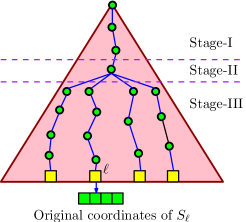
Figure 2: Global Structure

Skeleton of the structure. Consider the projection of the rectangles of $S$ on to the $xy$-plane and impose an orthogonal $\left\llbracket 2\sqrt{\frac{n}{\log^{4}n}}\right\rrbracket\times\left\llbracket 2\sqrt{\frac{n}{\log^{4}n}}\right\rrbracket$ grid such that each horizontal and vertical slab contains the projections of $\sqrt{n\log^{4}n}$ sides of $S$. This grid is the root node of our tree ${\cal T}$. For each vertical and horizontal slab, we recurse on the rectangles of $S$ which are sent to that slab. At each node of the recursion tree, if we have $m$ rectangles in the subproblem, the grid size changes to $\left\llbracket 2\sqrt{\frac{m}{\log^{4}m}}\right\rrbracket\times\left\llbracket 2\sqrt{\frac{m}{\log^{4}m}}\right\rrbracket$. We stop the recursion when a node has less than $w^{1/4}$ rectangles.

Breaking the rectangles.

The solution of Rahul [32] breaks only one side to reduce $5$-sided rectangles to $4$-sided rectangles, and then uses the solution for $4$-sided rectangle stabbing as a black box. Unlike the approach of Rahul [32], we will break two sides of each $5$-sided rectangle to obtain $O(\log\log n)$ $3$-sided rectangles.

For a node in the tree, the intersection of every pair of horizontal and vertical grid line defines a grid point. A rectangle $r\in S$ is associated with four root-to-leaf paths (as shown in Figure 2). Any node (say, $v$) on these four paths is classified w.r.t. $r$ into one of the three stages as follows:

Stage-I. The $xy$-projection of $r$ intersects none of the grid points. Then $r$ is not stored at $v$, and sent to the child corresponding to the row or column $r$ lies in.

Stage-II. The $xy$-projection of $r$ intersects at least one of the grid points. Then $r$ is broken into at most five disjoint pieces. The first piece is a grid rectangle, which is the bounding box of all the grid points lying inside $r$, as shown in Figure 3(b). The remaining four pieces are two column rectangles and two row rectangles as shown in Figure 3(c) and (d), respectively. The grid rectangle is stored at $v$. Note that each column rectangle (resp., row rectangle) is now a $4$-sided rectangle in $\mathbb{R}^{3}$ w.r.t. its column (resp., row), and is sent to its corresponding child node.

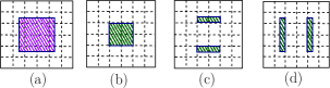
Figure 3: Breaking a $5$-sided rectangle in (a) into 2 horizontal side rectangles (shown in (c)) and 2 vertical side rectangles (shown in (d)).

Stage-III. The $xy$-projection of a $4$-sided piece of $r$ intersects at least one of the grid points. Without loss of generality, assume that the $4$-sided rectangle $r$ is unbounded along the negative $x$-axis. Then the rectangle is broken into at most four disjoint pieces: a grid rectangle, two row rectangles, and a column rectangle, as shown in Figure 4(b), (c) and (d), respectively. The grid rectangle and the two row rectangles are stored at $v$, and the column rectangle is sent to its corresponding child node. Note that the two row rectangles are now $3$-sided rectangles in $\mathbb{R}^{3}$ w.r.t. their corresponding rows (unbounded in one direction along $x$-, $y$- and $z$-axis).

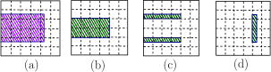
Figure 4: Breaking a $4$-sided rectangle in (a) into 2 horizontal side rectangles (shown in (c)) and 2 vertical side rectangles (shown in (d)).

Encoding structures. Let $S_{v}$ be the set of rectangles stored at a node $v$ in the tree. We apply a rank space reduction (replacing input coordinates by their ranks) so that the coordinates of all the endpoints are in $[2|S_{v}|]^{3}$. If $v$ is a leaf node, then we build an instance of Lemma 5. Otherwise, the following three structures will be built using $S_{v}$:

(A) Slow structure. An instance of Lemma 4 is built on $S_{v}$ to answer the 3-d $5$-sided rectangle stabbing query when the output size is “large”.

(B) Grid structure. For each cell $c$ of the grid, among the rectangles which completely cover $c$, pick the $\log^{3}|S_{v}|$ rectangles with the largest span along the $z$-direction. Store them in a list $\mathit{Top(c)}$ in decreasing order of their span.

(C) 3-d dominance structure. For a given row or column in the grid, based on the $3$-sided rectangles stored in it, a linear-space 3-d dominance reporting structure [1, 10] is built. This structure is built for each row and column slab.

Where are the original coordinates stored?

Unlike the previous approaches for indexing points [5, 11], we use a somewhat unusual approach for storing the original coordinates of each rectangle. In the process of breaking each $5$-sided rectangle described above, there will be four leaf nodes where portions of the rectangle will get stored. We will choose these leaf nodes to store the original coordinates of the rectangle (see Figure 2). The benefit is that each $3$-sided rectangle (stored at a node $v$) has to maintain a decoding pointer of length merely $O(\log|S_{v}|)$ to point to its original coordinates stored in its subtree.

Query algorithm and analysis.

Given a query point $q$, we start at the root node and perform the following steps: First, query the dominance structure corresponding to the horizontal and the vertical slab containing $q$. Next, for the grid structure, locate the cell $c$ on the grid containing $q$. Scan the list $\mathit{Top(c)}$ to keep reporting till (a) all the rectangles have been exhausted, or (b) a rectangle not containing $q$ is found. If case (a) happens and $|\mathit{Top(c)}|=\log^{3}|S_{v}|$, then we discard the rectangles reported till now, and query the slow structure. The decoding pointers will be used to report the original coordinates of the rectangles. Finally, we recurse on the horizontal and the vertical slab containing $q$. If we visit a leaf node, then we query the leaf structure (Lemma 5).

First, we analyze the space. Let $s(|S_{v}|)$ be the amortized number of bits needed per input $5$-sided rectangle in the subtree of a node $v$. The amortized number of bits needed per rectangle for the encoding structures and the pointers to the original coordinates is $O(\log|S_{v}|)$. This leads to the following recurrence:

$$s(n)=s(\sqrt{n\log^{4}n})+O(\log n)$$

which solves to $s(n)=O(\log n)$ bits. Therefore, the overall space is bounded by $O(n)$ words.

Next, we analyze the query time. To simplify the analysis, we will exclude the output size term while mentioning the query time. At the root, the time taken to query the grid and the dominance structure is $O(\log\log_{w}n)$. This leads to the following recurrence:

$$Q(n)=2Q(\sqrt{n\log^{4}n})+O(\log\log_{w}n)$$

with a base case of $Q(w^{1/4})=O(1)$. This solves to $Q(n)=O(\log_{w}n-\log\log_{w}n)=O(\log_{w}n)$. For each reported rectangle it takes constant time to recover its original coordinates. The time taken to query the slow structure is dominated by the output size. Therefore, the overall query time is $O(\log_{w}n+k)$.

Theorem 2

There is a data structure of size $O(n)$ words which can answer any 3-d $5$-sided rectangle stabbing query in $O(\log_{w}n+k)$ time. This is optimal in the word RAM model.

Our solution for 2-d top-$k$ rectangle stabbing can be found in Section E of the appendix.

3.3 3-d $6$-sided rectangle stabbing

In this section we will prove the following result.

Theorem 3

There is a linear-space data structure that answers 3-d rectangle stabbing queries in $O(\log^{2}_{w}n+k)$ time.

The complete discussion on $6$-sided rectangle stabbing is provided in Section F of the appendix. Here we will only highlight the key result.

Lemma 6

There exists a linear-space data structure that answers $z$-restricted 3-d $4$-sided rectangle stabbing queries in $O(\log w\cdot\log\log n+k)$ time. A $z$-restricted $4$-sided rectangle is of the form $(-\infty,x]\times(-\infty,y]\times[i,j]$, where integers $i,j\in\left[w^{\varepsilon}\right]$ and $\varepsilon=0.1$.

Lemma 7

There exists an optimal linear-space data structure that answers $z$-restricted 3-d 4-sided rectangle stabbing queries in $O(\log\log_{w}n+k)$ time. A $z$-restricted $4$-sided rectangle is of the form $(-\infty,x]\times(-\infty,y]\times[i,j]$, where integers $i,j\in\left[w^{\varepsilon}\right]$ and $\varepsilon=0.1$.

• Proof: We can safely assume that $n>w^{2\varepsilon}\cdot\log w\log\log n$, because the case of $n<w^{2\varepsilon}\cdot\log w\log\log n=O(w^{1/4})$ can be handled in $O(1+k)$ time by using the structure of Lemma 5. To keep the discussion short, we will assume that $k<\log w\cdot\log\log n$ (handling small values of $k$ is typically more challenging).

Shallow cuttings.

A point $p_{1}$ is said to dominate point $p_{2}$ if it has a larger $x$-coordinate and a larger $y$-coordinate value. Our main tool to handle this case are shallow cuttings which have the following three properties: (a) A $t$-shallow cutting for a set $P$ of 2-d points is a union of $O(n/t)$ cells where every cell is of the form $[a,+\infty)\times[b,+\infty)$, (b) every point that is dominated by at most $t$ points from $P$ will lie within some cell(s), and (c) each cell contains at most $O(t)$ points of $P$. A cell $[a,+\infty)\times[b,+\infty)$ can be identified by its corner $(a,b)$. We denote by $\textit{Dom}(c)$ the set of points that dominate the corner $c$.

Data structure.

We classify rectangles according to their $z$-projections. The set $S_{ij}$ contains all rectangles of the form $r=(-\infty,x_{f}]\times(-\infty,y_{f}]\times[i,j]$. Since $1\leq i\leq j\leq w^{\varepsilon}$, there are $O(w^{2\varepsilon})$ sets $S_{ij}$. Every rectangle $r$ in $S_{ij}$ is associated with a point $p(r)=(x_{f},y_{f})$. We construct a $t$-shallow cutting $L_{ij}$ with $t=\log w\cdot\log\log n$ for the set of points $p(r)$, such that $r\in S_{ij}$. A rectangle $r=(-\infty,x_{f}]\times(-\infty,y_{f}]\times[i,j]$ is stabbed by a query point $q=(q_{x},q_{y},q_{z})$ if and only if $p(r)\in S_{ij}$ and the point $p(r)$ dominates the 2-d point $(q_{x},q_{y})$. We can find points of a set $S_{ij}$ that dominate $q$ using the shallow cutting $L_{ij}$. However, to answer the stabbing query we must simultaneously answer a dominance query on $O(w^{2\varepsilon})$ different sets of points.

We address this problem by grouping corners of different shallow cuttings into one structure. Let $\mathcal{C}_{ij}$ denote the set of corners in a shallow cutting $L_{ij}$ and let $\mathcal{C}=\bigcup_{\forall i,j\in[w^{\varepsilon}]}\mathcal{C}_{ij}$. The set $\mathcal{C}$ is divided into disjoint groups, so that every group $G_{\alpha}$ consists of $w^{2\varepsilon}$ consecutive corners (with respect to their $x$-coordinates): for any $c\in G_{\alpha}$ and $c^{\prime}\in G_{\alpha+1}$, $c.x<c^{\prime}.x$. We say that a corner $c\in\mathcal{C}_{ij}$ is immediately to the left of $G_{\alpha}$ if it is the rightmost corner in $\mathcal{C}_{ij}$ such that $c_{x}\leq c^{\prime}_{x}$ for any corner $c^{\prime}=(c^{\prime}_{x},c^{\prime}_{y})$ in $G_{\alpha}$. The set of corners $\overline{G}_{\alpha}$ contains (1) all corners from $G_{\alpha}$, and (2) for every pair $i,j$ such that $1\leq i\leq j\leq w^{\varepsilon}$, the corner $c\in\mathcal{C}_{ij}$ immediately to the left of $G_{\alpha}$. The set $R_{\alpha}$ contains all rectangles $r$ such that $p(r)\in\textit{Dom}(c)$ for each corner $c\in\overline{G}_{\alpha}$. Since $R_{\alpha}$ contains $O(w^{2\varepsilon}\log w\cdot\log\log n)=O(w^{1/6})$ rectangles, we can perform a rank-space reduction and answer queries on $R_{\alpha}$ in $O(k+1)$ time by using Lemma 5; see Fig. 5.

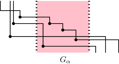
Figure 5: The set of corners $G_{\alpha}$

Next, we will show that the space occupied by this structure is $O(n)$. The crucial observation is that the number of corners in $G_{\alpha}$ is $w^{2\varepsilon}$ and the number of “immediately left” corners added to each $\overline{G}_{\alpha}$ is also bounded by $w^{2\varepsilon}$. The number of corners in set $\mathcal{C}$ is bounded by $\sum_{\forall L_{i,j}}O\left(1+\frac{|S_{ij}|}{t}\right)=O(n/t)$, since $n/t>w^{2\varepsilon}$. Therefore, the number of groups will be $O\left(\frac{n}{tw^{2\varepsilon}}\right)$. Each set $R_{\alpha}$ contains $O(w^{2\varepsilon}t)$ rectangles. Therefore, the total space occupied by this structure is $\sum_{\forall\alpha}|R_{\alpha}|=O(\frac{n}{tw^{2\varepsilon}}\cdot w^{2\varepsilon}t)=O(n)$.

Query algorithm.

Given a query point $q=(q_{x},q_{y},q_{z})$, we find the set $G_{\alpha}$ that “contains” $q_{x}$. Then we report all the rectangles in $R_{\alpha}$ that are stabbed by $q$ by using Lemma 5. We need $O(\log\log_{w}n)$ time to find the group $G_{\alpha}$ [31] and, then $O(1+k)$ time to report $R_{\alpha}\cap q$.

Our procedure reports all rectangles stabbed by the query point: Suppose that a point $q$ stabs at most $t$ rectangles. Let $G_{\alpha}$ denote the group of corners that contains $q$. If $q$ stabs a rectangle $r$, then $p(r)$ dominates $q$. Hence $p(r)\in\textit{Dom}(c)$ for some corner $c\in\overline{G}_{\alpha}$ and the rectangle $r$ is stored in the data structure $R_{\alpha}$. Now suppose that $q$ stabs more than $t$ rectangles. Then, by the same token, there are at least $t$ rectangles in $R_{\alpha}$ that are stabbed by $q$. Hence we will use the slow data structure to answer the query and correctly report all rectangles in this case.    $\Box$

Appendix

Appendix A On the Models

Throughout this paper, the pointer machine model refers to the “arithmetic pointer machine” (APM) in the terminology from Chazelle’s paper [14]: Each word (or memory cell) stores a constant number of pointers, input points, and/or $w$-bit integers for a fixed $w$. We support pointer chasing and standard arithmetic operations, comparisons, and shifts on $w$-bit integers in unit time each, but do not allow pointer arithmetic. It is assumed that $w\geq\log n$ (which is reasonable since a pointer or input point requires $\Omega(\log n)$ bits).

In the I/O model, each block is assumed to hold $B$ words for a fixed $B$, where each word stores an input point or a $w$-bit integer, again assuming that $w\geq\log n$. We support block reads/writes with unit cost each; all other operations on a block are free.

In the word RAM model, each word stores a $w$-bit integer, again assuming that $w\geq\log n$; we support standard arithmetic operations, comparisons, bitwise logical operations, and shifts on $w$-bit integers in unit time each, and allow these $w$-bit integers to be used as pointers. Furthermore, it is assumed that the coordinates of the input points are $w$-bit integers.

Appendix B Proof of Lemmata 1 and 2

For Lemma 1, such data structures for 2-d orthogonal point location can be found in [26, 25, 16, 36, 39] for the pointer machine model, [21, 6] for the I/O model, and [10] for the word RAM model. For Lemma 2, 2-d rectangle stabbing emptiness (or more generally, rectangle stabbing counting) is known to be reducible to 2-d orthogonal range counting [18], and such data structures for 2-d orthogonal range counting can be found in [14] for the pointer machine model, [22] for the I/O model, and [24] for the word RAM model.

All these known data structures technically require $O(n)$ words of space, or more precisely, $O(n\log U)$ bits of space. In the I/O model or word RAM model, we can easily pack the data structures in $O\left(\frac{n\log U}{w}\right)$ words of space without increasing the query cost when $\log U\ll w$. In the pointer machine model, we may not be able to pack the data structures in general, since if multiple “micro-pointers” are packed in a word, the model does not allow us to follow such a micro-pointer. Nevertheless, it is not difficult to modify the existing data structures to achieve the compressed space bound; next, we present the technical details of the modifications needed.

Proof of Lemma 1 for pointer machines.

For 2-d orthogonal point location, one solution is via $(1/r)$-cuttings [20]: we can partition the plane into $O(r)$ disjoint rectangular cells, each intersecting $O(n/r)$ line segments (edges of the input rectangles), where we choose $r=\frac{\delta n\log U}{w}$ for a sufficiently small constant $\delta$.

We build a point location structure [26, 25, 16, 36, 39] for the $O(r)$ cells with $O(\log r)$ query time in the pointer machine model; the space usage of this structure in words is $O(r)$, which is within the allowed bound $O\left(\frac{n\log U}{w}\right)$, so there is no need for bit packing here.

For each cell, we store the $O(n/r)$ line segments in a point location structure [25] with $O\left(\log(n/r)\right)$ query time; the space usage of this structure in bits is $O\left((n/r)\log U\right)$, which is $O\left(\delta w\right)$, so the entire structure can be packed in a single word. Although pointer chasing is not directly supported in the pointer machine model when multiple “micro-pointers” are packed in a word, we can simulate each pointer chasing step here in constant time by arithmetic operations and shifts within the word.

Given a query point $q$, we can first find the cell containing $q$ in $O\left(\log r\right)$ time and then finish the query inside the cell in $O\left(\log(n/r)\right)$ time. The overall query time is $O\left(\log n\right)$.

Proof of Lemma 2 for pointer machines.

Rectangle stabbing emptiness in 2-d reduces to dominance range counting in 2-d [18]. Chazelle’s compressed range tree structure [14] solves the latter problem with $O(n)$ words of space and $O(\log n)$ time in the pointer machine model. We observe that his data structure actually achieves $O\left(\frac{n\log U}{w}\right)$ words of space, after minor modifications.

At each level of the range tree, Chazelle’s structure stores lists consisting of a total of $O\left(\frac{n}{w}\right)$ words ($O\left(\frac{n}{w}\right)$ $w$-bit integers as well as $O\left(\frac{n}{w}\right)$ pointers to words in lists at the next level). The total number of words over all levels of the tree is $O\left(\frac{n\log n}{w}\right)\leq O\left(\frac{n\log U}{w}\right)$.

We shorten the tree by making the leaf nodes contain $b$ points, where we choose $b=\frac{\delta w}{\log U}$ for a sufficiently small constant $\delta$. This way, the space in words for the tree itself is $O\left(n/b\right)=O\left(\frac{n\log U}{w}\right)$. Inside each leaf, we store the $b$ points in another instance of Chazelle’s structure; the space usage of this structure in bits is $O\left(b\log U\right)$, which is $O\left(\delta w\right)$, so the entire structure can be packed in a single word. Again, we can simulate each pointer chasing step here in constant time by arithmetic operations and shifts within the word.

To answer a dominance range counting query, we descend along a path in the compressed range tree, which requires $O(\log(n/b))$ time by following pointers in the lists stored at the path and doing various arithmetic operations and shifts on $w$-bit integers. At the leaf of the path, we can finish the query in $O\left(\log b\right)$ time. The overall query time is $O\left(\log n\right)$.

Appendix C Other Models

In the I/O model, the analysis is similar, with a modified recurrence for the query cost:

$$Q\left(U,U,U\right)=Q\left(\sqrt{U},\sqrt{U},\sqrt{U}\right)+O\left(\log_{B}U\right).$$

For the base case $U\leq B^{1/3}$, we have $Q\left(U,U,U\right)=O(1)$ trivially, since $n\leq U^{3}\leq B$. Solving the recurrence yields $O\left(\log_{B}N\right)$ query cost. The space usage remains $O\left(N\right)$ words (i.e., $O\left(N/B\right)$ blocks).

In the word RAM model, the analysis is again similar, with

$$Q\left(U,U,U\right)=Q\left(\sqrt{U},\sqrt{U},\sqrt{U}\right)+O\left(\log_{w}U\right).$$

For the base case $U\leq w$, we have $Q\left(U,U,U\right)=O\left(1\right)$ by switching to another known method: Orthogonal point location in 3-d reduces to 6-d dominance emptiness, for which there is a known method [12] with $O\left(n(\log_{w}n)^{4}\right)$ words of space and $O\left((\log_{w}n)^{5}\right)$ query time in the word RAM. (The method in [12] can be modified to report a witness if the range is non-empty.) Since $n\leq U^{3}\leq w^{3}$, we have $\log_{w}n=O(1)$, and so the space bound is $O\left(n\right)$ and query bound is $O\left(1\right)$ for the base case. Solving the recurrence yields $O\left(\log_{w}N\right)$ query time.

Appendix D Final Remarks

Orthogonal point location in 4-d.

In the word RAM model, if we plug in the bounds for 3-d 6-sided rectangle stabbing (Theorem 7) and the bounds for 3-d orthogonal point location (Theorem 1) into our framework, then we obtain a linear-space structure which can answer a 4-d orthogonal point location query in $O(\log_{w}^{2}n)$ time.

Higher dimensions.

The same approach can be extended to higher dimensions, reducing the complexity of $d$-dimensional orthogonal point location to that of $(d-1)$-dimensional box stabbing emptiness. However, known data structures for higher-dimensional box stabbing [3] requires superlinear space, whereas the simpler approach mentioned in the Introduction, of using interval trees to reduce the dimension, gives $O\left(\log^{d-2}n\right)$ query time while keeping linear space in the pointer machine model.

The case of 3-d subdivisions.

Our approach can also be used to improve the space bound of de Berg, van Kreveld, and Snoeyink’s point location structure [15] for 3-d orthogonal subdivisions, from $O\left(n\log\log U\right)$ space to $O\left(n\right)$, in the word RAM model.

Theorem 4

Given a subdivision formed by $n$ disjoint (space-filling) axis-aligned boxes in 3-d, there is a data structure for point location with $O\left(n\right)$ words of space and $O\left(\log^{2}\log U\right)$ query time in the word RAM model.

• Proof: (Sketch)  De Berg et al.’s method [15, Theorem 2.4] was already based on a van Emde Boas recursion, partitioning along the $x$-direction. They also used 2-d orthogonal point location structures during the recursion, but managed to avoid rectangle stabbing structures by exploiting the fact that the input is a subdivision. Roughly, for each slab, they took the “holes” formed by all middle boxes that intersect the slab, and filled the holes by taking the vertical decomposition of the $yz$-projection. The analysis followed by charging the complexity of the decomposition to vertices within the slab.

  Our new change is to do the van Emde Boas recursion not just along the $x$-direction but along all three axis directions in a round-robin fashion. This leads to the same recurrence for space as in Section 2. The query time satisfies the following recurrence:

  $$Q\left(U,U,U\right)=Q\left(\sqrt{U},\sqrt{U},\sqrt{U}\right)+O\left(\log\log U\right).$$

  This leads to $O(\log^{2}\log U)$ query time.    $\Box$

Appendix E Top-$k$ 2-d rectangle stabbing

Our solution for $5$-sided rectangle stabbing can be modified to support top-$k$ stabbing queries in optimal time. We use the same general approach, but we need additional ideas to handle the top-$k$ aspect of the problem.

E.1 Top-$k$ 2-d dominance query

First, we will present an optimal solution for the top-$k$ 2-d dominance query where the input is a set $P$ of $n$ weighted points in 2-d, and the query is an integer $k$ and a dominance range $q=[q_{x},\infty)\times[q_{y},\infty)$. The result obtained is the following.

Theorem 5

There exists a linear-space data structure that answers the top-$k$ 2-d dominance query in $O(\log\log_{w}n+k)$ time. This is optimal in the word RAM model.

Preliminaries.

The optimality of Theorem 5 follows from the lower bound of Patrascu and Thorup for the predecessor search problem [31]. We will need the following two building blocks for our solution.

Lemma 8

(Patil et al.[28], Theorem 9) There exists a linear-space data structure that answers the top-$k$ 2-d dominance query in $O(\log n+k)$ time. The points are reported in a sorted order.

Lemma 9

We can keep $m=\log^{1/3}n$ points in a data structure of size $O(m)$-words that answers the top-$k$ 2-d dominance query in $O(1+k)$ time.

• Proof: First, we reduce the problem to rank space. Next, we build an instance of Lemma 8 on the rank-reduced dataset. Finally, since there are only $O(m^{2})$ combinatorially different queries we store $\log\log n$ highest weighted points that dominate each query point. As explained in the proof of Lemma 5 we can keep all pre-computed solutions in $O(m)$ words.

  To answer a query, the case of $k<\log\log n$ is handled by using the pre-computed solution, and the case of $k>\log\log n$ is handled in $O(\log\log n+k)=O(k)$ time by querying the structure of Lemma 8.    $\Box$

Shallow cuttings.

We will re-define shallow cuttings in the context of 3-d points. A point $p_{1}$ is said to dominate point $p_{2}$ if it has a larger coordinate value in all the three dimensions. A $t$-shallow cutting for a set $P$ of 3-d points is a collection of boxes of the form $[a,+\infty)\times[b,+\infty)\times[c,+\infty)$, such that (a) there are only $O(n/t)$ boxes, (b) every point that is dominated by at most $t$ points from $P$ will lie within some box, and (c) each box contains at most $O(t)$ points of $P$. A box $[a,+\infty)\times[b,+\infty)\times[c,\infty)$ can be identified by its corner $(a,b,c)$.

A common operation on a shallow cutting is FIND-ANY: Given a 3-d point $q^{\prime}$, find any box in the shallow cutting which contains $q^{\prime}$. The standard implementation of this query leads to a planar subdivision in the x-y plane consisting of orthogonal rectangles where each rectangle is labeled by a box in the shallow cutting. Now given a point $q^{\prime}(q_{x},q_{y},q_{z})$, we first perform a point location query on the planar subdivision with $(q_{x},q_{y})$.

If $B$ is the label on the rectangle and if $B$ contains $q$, then we report $B$; otherwise, we can safely conclude that no box contains $q$.

Data structure.

Our structure consists of the following components:
(A) Slow structure. Based on the pointset $P$, we build the data structure of Lemma 8.
(B) $\log n$-level shallow cutting. We regard the weights of the points of $P$ as the third coordinate and construct a $\log n$-shallow cutting $\mathcal{P}_{1}$.
(C) Slow structure for each box. The conflict list, $CL_{B}$, of a box $B\in\mathcal{P}_{1}$ is the points in $P$ which lie inside it. For each $CL_{B}$ the data structure of Lemma 8 is constructed.
(D) $\log^{1/3}n$-level shallow cutting. A $\log^{1/3}n$-shallow cutting $\mathcal{P}_{2}$ is constructed based on points in $P$.
(E) Small-sized structures. For every box in $\mathcal{P}_{2}$, based on its conflict list build the structure of Lemma 9.

The properties of the shallow cuttings and the fact that Lemma 8 and Lemma 9 are linear-space structures ensures that the space occupied by our data structure is $O(n)$ words.

Query algorithm.

We divide the query algorithm into three cases:
(A) $k\geq\log n$: Then we query the slow structure.
(B) $k\in[\log^{1/3}n,\log n]$: Then we perform the FIND-ANY operation on the $\log n$-shallow cutting $\mathcal{P}_{1}$ to find a box $B$ whose projection contains $q$, and then query the slow structure built on $CL_{B}$.
(C) $k\in[1,\log^{1/3}n]$: Then we perform the FIND-ANY operation on the $\log^{1/3}n$-shallow cutting $\mathcal{P}_{2}$ to find a box $B$ whose projection contains $q$, perform a rank-space reduction of the query w.r.t. to $CL_{B}$, and then query the small-sized structure built on $CL_{B}$.

We need $O(\log\log_{w}n)$ time to answer the FIND-ANY operation [10]. All the other steps take $O(k)$ time. Thus the total query time is $O(\log\log_{w}n+k)$.

Proof of correctness.

Assume that $k\in[\log^{1/3}n,\log n]$. Given a query point $q(q_{x},q_{y})$, let $q^{\prime}=(q_{x},q_{y},q_{z})$ be a point such that there are exactly $k$ points in $P\cap q^{\prime}$. Then it is guaranteed that there exists a box in the $\log n$-shallow cutting which will contain $q^{\prime}$. The implementation of the FIND-ANY operation ensures that the box $B$ returned by it will contain $q^{\prime}$. Therefore, the top-$k$ points of $P\cap q$ will be present in the conflict list of $B$. A similar argument holds for $k<\log^{1/3}n$.

Remark.

In the query algorithm, we assumed that $|S\cap q|\geq k$. This is easy to check by reporting the points in $S\cap q$ till one of the following happens: either $k+1$ points are reported or all the points are reported.

E.2 Top-$k$ 2-d rectangle stabbing

Now we are ready to prove the following result.

Theorem 6

There is a linear-space data structure that can answer any top-$k$ 2-d rectangle stabbing query in $O(\log_{w}n+k)$ time. This is optimal in the word RAM model.

Preliminaries.

As in the case of top-$k$ 2-d dominance query, we will need a slow structure and a small-sized structure.

Lemma 10

There is a linear-space data structure which can answer any top-$k$ 2-d rectangle stabbing query in $O(\log^{2}n\cdot\log\log_{w}n+k)$ time.

• Proof: It is known that we can answer a 3-d 5-sided rectangle stabbing query by querying $O(\log^{2}n)$ 3-d dominance reporting structures [32]. The space of the data structure is within the same bounds as the 3-d dominance reporting structure. Refer to [32] for further details.

  In the same way, we can answer a 2-d top-$k$ rectangle stabbing query by querying $\log^{2}n$ top-$k$ 2-d dominance queries. We will return the $k$ heaviest points in sorted order using the same technique that will be used later in this section.    $\Box$

Lemma 11

We can keep $m=w^{1/4}$ points in a data structure of size $O(m)$-words that answers the top-$k$ 2-d rectangle stabbing query in $O(1+k)$ time.

All the above data structures (Theorem 5, Lemma 10, and Lemma 11) support queries in an online manner. That is, we do not need to know the value of $k$ when the query is asked, since the elements are reported in descending order of their weights. The procedure can be paused and resumed at a later time.

Data structure.

We only worry about $k<\log^{3}n$, since the other case can be optimally handled by Lemma 10. We use the same structure as in the proof of Theorem 2 with the following differences: we use top-$k$ 2-d dominance structure of Theorem 5 instead of the 3-d dominance structure, and we use the slow data structure of Lemma 10 instead of the slow structure of Lemma 4. Now $Top(c)$ is the $\log^{3}|S_{v}|$ heaviest rectangles among the rectangles covering the grid cell $c$ and is stored in decreasing order of their weight. Finally, the leaf structure is built by using Lemma 11.

Query algorithm.

Consider the following abstract problem: We are given sorted lists $L_{1},L_{2},\ldots,L_{t}$ such that the total number of elements in all the lists is less than or equal to $n$, and $t=O(\log_{w}n)$. The goal is to report the $k$ heaviest elements. To answer this, we build a heap $\mathcal{G}$ based on the heaviest element from each list. Now we perform the following operations on $\mathcal{G}$ $k$ times: (a) delete the element, $e$, with the largest weight and report it, and (b) if $e$ came from list $L_{i}$, then insert the next heaviest element from $L_{i}$ into $\mathcal{G}$. We implement $\mathcal{G}$ as a fusion tree [19]; since $\mathcal{G}$ contains at most $\log_{w}n$ elements, all operations on $\mathcal{G}$ are supported in $O(1)$ time.

By now the reader must have guessed the query algorithm.
(A) Identify the $O(\log_{w}n)$ nodes as explained in Section 3.2.
(B) Each identified node acts a list $L_{i}$ (as discussed before, the grid structure and the top-$k$ 2-d dominance structure can report in an online manner. If more than $\log^{3}|S_{v}|$ rectangles have been reported from a node $v$, then we switch to its slow structure).
(C) Now find the top-$k$ heaviest rectangles in $S\cap q$.

Appendix F 3-d 6-sided rectangle stabbing

In this section we will fill the missing details for the proof of the following result.

Theorem 7

There is a linear-space data structure that answers 3-d rectangle stabbing queries in $O(\log^{2}_{w}n+k)$ time.

F.1 Skeleton structure

Data structure.

We construct an interval tree, $IT$, with fan-out $w^{\varepsilon}$ on the $z$-projections of rectangles in $S$ for a positive constant $\varepsilon<1/18$. For a node $v\in IT$, let $\ell(v_{i})$ denote the bounding planes of its children and let $z_{i}(v)$ be the $z$-coordinate of $\ell(v_{i})$. The set $S(v)\subseteq S$ contains all rectangles $[x_{1},x_{2}]\times[y_{1},y_{2}]\times[z_{1},z_{2}]$, such that $v$ is the lowest common ancestor of the leaves storing $z_{1}$ and $z_{2}$. We keep three stabbing data structures $M(v)$, $L(v)$, and $R(v)$ at each node $v$. Consider an arbitrary rectangle $r=[x_{1},x_{2}]\times[y_{1},y_{2}]\times[z_{1},z_{2}]$ stored in $S(v)$. Suppose that $z_{k}(v)<z_{1}\leq z_{k+1}(v)$ and $z_{l-1}(v)\leq z_{2}<z_{l}(v)$. If $k+1<l-1$, we store a rectangle $[x_{1},x_{2}]\times[y_{1},y_{2}]\times[k+1,l-1]$ in a data structure $M(v)$. We also store $r$ in data structures $R(v_{k})$ and $L(v_{l})$. The $z$-coordinates of all rectangles in $M(v)$ lie in the integer universe $[w^{\varepsilon}]$. We will use this fact to answer rectangle stabbing queries in $O(\log_{w}n+k)$ time, as will be shown later in this section in Theorem 8. Rectangles stored in $L(v)$ and $R(v)$ cross the left or the right bounding plane of the node $v$. Hence we can treat the rectangles in $L(v)$ (resp. $R(v)$) as 5-sided rectangles. Using Theorem 2, we can answer stabbing queries on $R(v)$ and $L(v)$ in $O(\log_{w}n+k)$ time.

Query algorithm.

To report all rectangles that stab a point $q$, we traverse a root-to-leaf path in $IT$ and answer stabbing queries using data structures built for $L(v)$, $R(v)$ and $M(v)$ in each node $v$. Since the length of a root-to-leaf path is $O(\log_{w}n)$, the query is answered in $O(\log^{2}_{w}n+k)$ time

F.2 $z$-restricted queries

It remains to show how to answer 3-d rectangle stabbing queries when the $z$-coordinates of the endpoints are bounded by the integer universe $[w^{\varepsilon}]$. This scenario will be called $z$-restricted queries.

Lemma 12

There exists a linear-space data structure that answers $z$-restricted $4$-sided rectangle stabbing queries in $O(\log w\cdot\log\log n+k)$ time.

• Proof: We construct a (binary) interval tree $\mathcal{T}_{z}$ on the $z$-projections of the rectangles. Every leaf of this tree corresponds to a $z$-coordinate in the universe $[w^{\varepsilon}]$. Since $\mathcal{T}_{z}$ has $w^{\varepsilon}$ leaves, its height is $\log w^{\varepsilon}=O(\log w)$. Each rectangle is stored at a particular node in the tree and for each node we build two data structures that support 3-d dominance reporting queries. See e.g., Rahul [32] for a detailed description about the construction of the data structure. A stabbing query can be answered by traversing a path from the root of $\mathcal{T}$ to a leaf node. Since a 3-d dominance reporting query can be answered in $O(\log\log n+k)$ time and we visit $O(\log w)$ nodes, the total time needed to answer a query is $O(\log w\cdot\log\log n+k)$.    $\Box$

Lemma 13

There exists a linear-space data structure that answers $z$-restricted 4-sided 3-d rectangle stabbing queries in $O(\log\log_{w}n+k)$ time.

• Proof: Lemma 7 (in the main body of the paper) proves this lemma for the case $k<\log w\cdot\log\log_{w}n$. To handle the case of $k\geq\log w\log\log_{w}n$, we will use Lemma 12.

  $\Box$

Now we turn our attention to $z$-restricted $6$-sided rectangle stabbing queries. In this case, the data structure contains $6$-sided rectangles, but again the $z$-coordinates of the endpoints lie in the integer universe $[w^{\varepsilon}]$.

Lemma 14

There exists a linear-space data structure that answers $z$-restricted six-sided rectangle stabbing queries in $O(\log n+k)$ time.

• Proof: Again we use a binary interval tree on the $z$-projections of the rectangles, then assign each rectangle to a particular node in the tree, and then build two data structures at each node which will answer 5-sided rectangle stabbing queries. When we answer a $6$-sided query, we traverse a root-to-leaf path and answer a 5-sided query at every node. We refer the reader to [32] or [29] for a complete description. The height of the tree is $O(\log w)$ and, by Theorem 2 we need $O(\log_{w}n)$ time to answer a 5-sided query. Hence the overall time it takes to answer a $z$-restricted six-sided query is $O(\log n)$.    $\Box$

Theorem 8

There exists a linear-space data structure that answers a $z$-restricted 6-sided rectangle stabbing query in $O(\log_{w}n+k)$ time.

• Proof: We use the approach as in Theorem 2, but use different encoding structures.
  (A) Slow structure. An instance of Lemma 14 is built on $S_{v}$.
  (B) Grid structure. For every cell $c$ we keep lists $\mathit{Cover(c,z)}$ for $z=1$, $\ldots$, $w^{\varepsilon}$; $\mathit{Cover(c,z)}$ contains $\log|S_{v}|$ rectangles $r$, such that the projection of $r$ onto the $xy$-plane completely covers $c$ and the $z$-projection of $r$ is stabbed by $z$.
  (C) “$z$-restricted dominance” structure. For a given row or column in the grid, based on the $z$-restricted 4-sided rectangles stored in it, an instance of Lemma 13 is built.

  The space and the query time analysis follow from the analysis of Theorem 2.    $\Box$

References

- [1] Peyman Afshani. On dominance reporting in 3D. In Proceedings of European Symposium on Algorithms (ESA), pages 41–51, 2008.
- [2] Peyman Afshani, Lars Arge, and Kasper Dalgaard Larsen. Orthogonal range reporting: query lower bounds, optimal structures in 3-d, and higher-dimensional improvements. In Proceedings of Symposium on Computational Geometry (SoCG), pages 240–246, 2010.
- [3] Peyman Afshani, Lars Arge, and Kasper Green Larsen. Higher-dimensional orthogonal range reporting and rectangle stabbing in the pointer machine model. In Proceedings of Symposium on Computational Geometry (SoCG), pages 323–332, 2012.
- [4] Peyman Afshani, Gerth Stølting Brodal, and Norbert Zeh. Ordered and unordered top-k range reporting in large data sets. In Proceedings of the Annual ACM-SIAM Symposium on Discrete Algorithms (SODA), pages 390–400, 2011.
- [5] Stephen Alstrup, Gerth Stølting Brodal, and Theis Rauhe. New data structures for orthogonal range searching. In Proceedings of Annual IEEE Symposium on Foundations of Computer Science (FOCS), pages 198–207, 2000.
- [6] Lars Arge, Andrew Danner, and Sha-Mayn Teh. I/O-efficient point location using persistent B-trees. ACM Journal of Experimental Algorithmics, 8, 2003.
- [7] J.L. Bentley. Solutions to Klee’s rectangle problems. Technical Report, Carnegie-Mellon University, Pittsburgh, PA, 1977.
- [8] Gerth Stølting Brodal. External memory three-sided range reporting and top- queries with sublogarithmic updates. In Proceedings of Symposium on Theoretical Aspects of Computer Science (STACS), volume 47, pages 23:1–23:14. 2016.
- [9] Gerth Stølting Brodal, Rolf Fagerberg, Mark Greve, and Alejandro Lopez-Ortiz. Online sorted range reporting. In International Symposium on Algorithms and Computation (ISAAC), pages 173–182, 2009.
- [10] Timothy M. Chan. Persistent predecessor search and orthogonal point location on the word RAM. ACM Transactions on Algorithms, 9(3):22, 2013.
- [11] Timothy M. Chan, Kasper Green Larsen, and Mihai Pǎtraşcu. Orthogonal range searching on the RAM, revisited. In Proceedings of Symposium on Computational Geometry (SoCG), pages 1–10, 2011.
- [12] Timothy M. Chan and Gelin Zhou. Multidimensional range selection. In International Symposium on Algorithms and Computation (ISAAC), pages 83–92, 2015.
- [13] Bernard Chazelle. Filtering search: A new approach to query-answering. SIAM Journal of Computing, 15(3):703–724, 1986.
- [14] Bernard Chazelle. A functional approach to data structures and its use in multidimensional searching. SIAM Journal of Computing, 17(3):427–462, 1988.
- [15] Mark de Berg, Marc J. van Kreveld, and Jack Snoeyink. Two- and three-dimensional point location in rectangular subdivisions. Journal of Algorithms, 18(2):256–277, 1995.
- [16] Herbert Edelsbrunner, Leonidas J. Guibas, and Jorge Stolfi. Optimal point location in a monotone subdivision. SIAM Journal of Computing, 15(2):317–340, 1986.
- [17] Herbert Edelsbrunner, G. Haring, and D. Hilbert. Rectangular point location in d dimensions with applications. Comput. J., 29(1):76–82, 1986.
- [18] Herbert Edelsbrunner and Mark H. Overmars. On the equivalence of some rectangle problems. Information Processing Letters (IPL), 14(3):124–127, 1982.
- [19] Michael L. Fredman and Dan E. Willard. Surpassing the information theoretic bound with fusion trees. Journal of Computer and System Sciences (JCSS), 47(3):424–436, 1993.
- [20] Michael T. Goodrich, Mark W. Orletsky, and Kumar Ramaiyer. Methods for achieving fast query times in point location data structures. In Proceedings of the Annual ACM-SIAM Symposium on Discrete Algorithms (SODA), 1997.
- [21] Michael T. Goodrich, Jyh-Jong Tsay, Darren Erik Vengroff, and Jeffrey Scott Vitter. External-memory computational geometry. In Proceedings of Annual IEEE Symposium on Foundations of Computer Science (FOCS), pages 714–723, 1993.
- [22] Sathish Govindarajan, Pankaj K. Agarwal, and Lars Arge. CRB-tree: An efficient indexing scheme for range-aggregate queries. In Proceedings of International Conference on Database Theory (ICDT), pages 143–157, 2003.
- [23] John Iacono and Stefan Langerman. Dynamic point location in fat hyperrectangles with integer coordinates. In Proceedings of the Canadian Conference on Computational Geometry (CCCG), 2000.
- [24] Joseph JáJá, Christian Worm Mortensen, and Qingmin Shi. Space-efficient and fast algorithms for multidimensional dominance reporting and counting. In International Symposium on Algorithms and Computation (ISAAC), pages 558–568, 2004.
- [25] David G. Kirkpatrick. Optimal search in planar subdivisions. SIAM Journal of Computing, 12(1):28–35, 1983.
- [26] Richard J. Lipton and Robert Endre Tarjan. Applications of a planar separator theorem. SIAM Journal of Computing, 9(3):615–627, 1980.
- [27] Yakov Nekrich. I/O-efficient point location in a set of rectangles. In Latin American Symposium on Theoretical Informatics (LATIN), pages 687–698, 2008.
- [28] Manish Patil, Sharma V. Thankachan, Rahul Shah, Yakov Nekrich, and Jeffrey Scott Vitter. Categorical range maxima queries. In Proceedings of ACM Symposium on Principles of Database Systems (PODS), pages 266–277, 2014.
- [29] Manish Patil, Sharma V. Thankachan, Rahul Shah, Yakov Nekrich, and Jeffrey Scott Vitter. Categorical range maxima queries. In Proceedings of ACM Symposium on Principles of Database Systems (PODS), pages 266–277, 2014.
- [30] Mihai Pǎtraşcu. Unifying the landscape of cell-probe lower bounds. SIAM Journal of Computing, 40(3):827–847, 2011.
- [31] Mihai Pǎtraşcu and Mikkel Thorup. Time-space trade-offs for predecessor search. In Proceedings of ACM Symposium on Theory of Computing (STOC), pages 232–240, 2006.
- [32] Saladi Rahul. Improved bounds for orthogonal point enclosure query and point location in orthogonal subdivisions in . In Proceedings of the Annual ACM-SIAM Symposium on Discrete Algorithms (SODA), pages 200–211, 2015.
- [33] Saladi Rahul and Ravi Janardan. A general technique for top- geometric intersection query problems. IEEE Transactions on Knowledge and Data Engineering (TKDE), 26(12):2859–2871, 2014.
- [34] Saladi Rahul and Yufei Tao. On top-k range reporting in 2d space. In Proceedings of ACM Symposium on Principles of Database Systems (PODS), pages 265–275, 2015.
- [35] Saladi Rahul and Yufei Tao. Efficient top-k indexing via general reductions. In Proceedings of ACM Symposium on Principles of Database Systems (PODS), 2016.
- [36] Neil Sarnak and Robert Endre Tarjan. Planar point location using persistent search trees. Communications of the ACM (CACM), 29(7):669–679, 1986.
- [37] Cheng Sheng and Yufei Tao. Dynamic top-k range reporting in external memory. In Proceedings of ACM Symposium on Principles of Database Systems (PODS), 2012.
- [38] Qingmin Shi and Joseph JáJá. Novel transformation techniques using q-heaps with applications to computational geometry. SIAM Journal of Computing, 34(6):1474–1492, 2005.
- [39] Jack Snoeyink. Point location. In J. E. Goodman and J. O’Rourke, editors, Handbook of Discrete and Computational Geometry, pages 767–787. CRC Press, 2nd edition, 2004.
- [40] Yufei Tao. A dynamic I/O-efficient structure for one-dimensional top-k range reporting. In Proceedings of ACM Symposium on Principles of Database Systems (PODS), pages 256–265, 2014.