The out-equilibrium 2D Ising spin glass: almost, but not quite, a free-field theory

Abstract

We consider the spatial correlation function of the two-dimensional Ising spin glass under out-equilibrium conditions. We pay special attention to the scaling limit reached upon approaching zero temperature. The field-theory of a non-interacting field makes a surprisingly good job at describing the spatial shape of the correlation function of the out-equilibrium Edwards-Anderson Ising model in two dimensions.

1 Introduction.

The importance of characterizing the spatial range of spin-glass correlations has been long recognized, both under equilibrium [1, 2] and out-equilibrium conditions [3, 4, 5, 6, 7, 8, 9, 10, 11, 12, 13, 14, 15, 16, 17, 18, 19, 20, 21, 22]. These correlations may be characterized though the overlap-overlap correlation function (for definitions, see below Sect. 2). However, we still lack analytical control over the spatial shape of this correlation function, which is a great nuisance for numerical work.

Here, we study the overlap-overlap correlation function for the Ising spin glass in spatial dimension $D=2$ both as a function of time and of spatial separation. Our numerical analysis is performed on lattices large enough to be representative of the infinite system-size limit. The two dimensional Ising spin glass undergoes a $T=0$ phase transition, however we hope that our results would apply equally in Ising spin glasses above its lower critical dimension (which is believed to be $D\simeq 2.5$ [23]) in the paramagnetic phase. In fact, recent experiments on a film geometry [17, 24, 25, 21, 26] motivated us to undertake a large scale numerical simulation of the out-equilibrium dynamics of the $D=2$ spin glass [22]. These systems, for small times, will behave as if living in a spin glass phase, yet for larges times they will cross over to the dynamical critical behavior of the two dimensional Ising spin glass- a paramagnetic phase behavior. Our aim here is to present a more field-theoretically minded analysis of the correlation function, as compared with our previous phenomenological analysis [22].

It came to us as a real surprise that the Langevin dynamics for the free scalar-field makes an excellent job in describing the spatial dependence of the spin-glass correlations. Of course, at least in an equilibrium setting [27, 28], large-distance correlations in a paramagnetic phase (and the $D=2$ Ising spin glass has only a paramagnetic phase for $T>0$) should be given by free-field theory. What is a surprise is that free-field theory is very accurate also at short distances. Furthermore, in the large-time limit of an equilibrated system, free-field theory can be made virtually exact for the spin-glass through a logarithmic wave-function renormalization (because of the vanishing anomalous dimension [29]). In fact, we are able to parameterize in a very simple way the rather heavy corrections-to-scaling found in a previous equilibrium study [30].

The remaining part of this work is organized as follows. In Sect. 2 we shall describe the model and the basic spin-glass correlation function that we compute (for further technical details, see Ref. [22]). In Sect. 3 we elaborate on the implications of scale invariance for the spatial shape of the correlation function. The relationship between the spin-glass correlations and the free-field propagator is considered in equilibrium (Sect. 4) and out-equilibrium (sect. 5). Our conclusions are presented in Sect. 6. A number of results regarding the free-field propagator are derived and discussed in A.

2 Model and Observables

Our dynamic variables are Ising spins, $s{x}=\pm 1$, placed in the nodes of a square lattice of linear dimension $L$. Their interaction is given by the Edwards-Anderson Hamiltonian [31, 32] with nearest-neighbors couplings and periodic boundary conditions

$${\cal H}=-\sum_{\langle\mathitbf{x},\mathitbf{y}\rangle}J_{\mathitbf{x},\mathitbf{y}}s{x}s{y}\,.$$ (1)

We consider quenched disorder [33], which means that the couplings $J_{\mathitbf{x},\mathitbf{y}}$ are fixed once for all. The couplings are drawn from the bimodal probability distribution ($J_{\mathitbf{x},\mathitbf{y}}=\pm 1$ with equal probability). Every set $\{J_{\mathitbf{x},\mathitbf{y}}\}$ defines a sample. We have simulated $L=512$, which is large enough to be insensitive to the finite size effects (see Sect. 4). Notice that the $T=0$ phase transition is Universal (i.e. it is independent of the type of disorder, see for example Ref. [29]).

Our numerical protocol is as follows. We start from a fully disordered spin configurations (representative of infinite temperature), which is instantaneously placed at the working temperature $T$ at the initial time $t_{\mathrm{w}}=0$. A standard Metropolis dynamics at fixed $T$ follows. Our time unit is a full-lattice sweep, which roughly corresponds to one picosecond [34]. We have simulated a multi-spin code of a $L=512$ lattice for a wide range of temperatures ($0.5\leq T\leq 1.1$). The number of simulated samples has been 96. For each sample, we have run 256 replicas (for $T\geq 0.55$) or 264 replicas (for $T=0.5$).

The overlap correlation function (see Ref. [16] for a detailed discussion) is computed from the replica-field

$$q^{\alpha,\beta}(\mathitbf{x},t_{\mathrm{w}})=s^{(\alpha)}(\mathitbf{x},t_{\mathrm{w}})s^{(\beta)}(\mathitbf{x},t_{\mathrm{w}})\,,\quad(\alpha\neq\beta)\,.$$ (2)

The $\{s^{(\alpha)}(\mathitbf{x},t_{\mathrm{w}})\}$ are real replicas ($\alpha$ is the so called replica index): replicas with different replica indices evolve under the same set of couplings $\{J_{\mathitbf{x},\mathitbf{y}}\}$ but are otherwise statistically independent. Hence, our correlation function is

$$C_{4}(\mathitbf{r},t_{\mathrm{w}};T)=\overline{\langle q^{\alpha,\beta}(\mathitbf{x},t_{\mathrm{w}})q^{\alpha,\beta}(\mathitbf{x}+\mathitbf{r},t_{\mathrm{w}})\rangle}\,,$$ (3)

where one first take the average over the thermal noise and the initial conditions, denoted by $\langle\ldots\rangle$. The average over the random couplings, denoted by an overline, is only computed afterwards. We shall restrict ourselves to displacement vectors along one of the lattice axis [the choice between $\mathitbf{r}=(r,0)$ or $\mathitbf{r}=(0,r)$ is immaterial, so we average over the two], and use the shorthand $C_{4}(r,t_{\mathrm{w}})$ [16, 35].

We characterize the spatial range of correlations through the coherence length:

$$\xi_{k,k+1}(t_{\mathrm{w}})\equiv I_{k+1}(t_{\mathrm{w}})/I_{k}(t_{\mathrm{w}})\,,$$ (4)

computed by means of the integrals

$$I_{k}(t_{\mathrm{w}})\equiv\int_{0}^{\infty}\mathrm{d}\,r\ r^{k}C_{4}(r,t_{\mathrm{w}})\,.$$ (5)

Following recent work [20, 16, 14, 19, 22], we shall focus our attention in the $k=1$ length-estimate $\xi_{12}(t_{\mathrm{w}})$.

Eventually, we have been able to equilibrate the system, in the sense that the integrals $I_{k}(t_{\mathrm{w}})$ no longer depend on $t_{\mathrm{w}}$ (within errors). Of course, an infinite system never fully equilibrates. However, in the paramagnetic phase (and spin-glasses in $D=2$ have only a paramagnetic phase at $T>0$), we can rather think of equilibration up to distance $r$: for any fixed distance $r$ the $C_{4}(r,t_{\mathrm{w}})$ approaches its equilibrium limit $C_{4}^{\mathrm{eq}}(r)$ exponentially fast in $t_{\mathrm{w}}$, after a $r$-dependent time threshold is reached, see A.2. Given that the equilibrium propagator decays exponentially with distance, we can regard the system as equilibrated for all practical purposes once the $C_{4}(r,t_{\mathrm{w}})$ equilibrates up to a distance (say) $r=6\,\xi_{12}^{\mathrm{eq}}(T)$. It is therefore meaningful to study numerically

$$\xi_{12}^{\mathrm{eq}}(T)=\lim_{t_{\mathrm{w}}\to\infty}\xi_{12}(t_{\mathrm{w}},T)\,.$$ (6)

In our simulations, $\xi_{12}^{\mathrm{eq}}(T)$ ranges from $\xi_{12}^{\mathrm{eq}}(T=1.1)\approx 4.3$ to $\xi_{12}^{\mathrm{eq}}(T=0.5)\approx 39.4$: this is why we expect that $L=512$ is large enough to accommodate $L\to\infty$ conditions [14, 19, 22].

In fact, if one takes first the limit $L\to\infty$ and only afterwards goes to low $T$, we expect a critical point at $T=0$:

$$\xi_{12}^{\mathrm{eq}}(T)\sim T^{-\nu}+\ldots,\quad 1/\nu=-\theta\,$$ (7)

where the dots stand for (rather complex [29]) subleading corrections to scaling. The stiffness exponent $\theta$ has been computed in a $T=0$ simulation for Gaussian-distributed couplings, $\theta=-0.2793(3)$ [36] (the identity $-\theta=1/\nu$, was already confirmed in former Gaussian couplings simulations, see for example Refs. [37, 29]). We have checked in [22] that Eq. (7) holds as well, with the same $\theta$, for our $J=\pm 1$ couplings.

Some readers may be unfamiliar with our coherence-length estimators, so let us relate our $\xi_{k,k+1}$ to the second-moment correlation length which is commonly studied in the context of equilibrium critical phenomena [38, 28]. Let $\hat{C}_{4}(\mathitbf{p},t_{\mathrm{w}})$ be the Fourier transform of $C_{4}(\mathitbf{r},t_{\mathrm{w}})$. In the thermodynamic limit $L\to\infty$, the momentum $\mathitbf{p}$ is a continuous variable. In the presence of rotational invariance (a reasonable assumption even for a fairly small $\xi_{12}(t_{\mathrm{w}})$ [16]), $\hat{C}_{4}$ depends on the squared momentum $p^{2}$. Hence, the second moment correlation length is

$$\xi^{\mathrm{2nd-moment}}=\sqrt{-\left.\frac{\partial\log\hat{C}_{4}}{\partial p^{2}}\right|_{p^{2}=0}}\,.$$ (8)

Eq. (8) can be conveniently adapted to a finite lattice, hence discrete $\mathitbf{p}$ [38, 39, 28], which partly explains its popularity. In real space, and assuming again $L\to\infty$ and rotational invariance, Eq. (8) reads in dimension $D$

$$\xi^{\mathrm{2nd-moment},D}=\sqrt{\frac{1}{2D}\,\frac{I_{D+1}}{I_{D-1}}}=\sqrt{\frac{\xi_{D-1,D}\,\xi_{D,D+1}}{2D}}\,.$$ (9)

The rationale for preferring $\xi_{12}$ over the more familiar $\xi^{\mathrm{2nd-moment},D}$ is a practical one [16]: statistical errors grow heavily with the index $k$ of the requested integrals $I_{k}$.

For later use, we note as well that the (equilibrium) spin-glass susceptibility is

$$\chi=\sum_{x,y=-\infty}^{\infty}C_{4}^{\mathrm{eq}}(x,y)\approx\ 2\pi I_{1}^{\mathrm{eq}}\,,$$ (10)

where we have assumed again rotational invariance, as well as $\xi_{12}^{\mathrm{eq}}\gg 1$, in order to approximate the double summation by the integral $I_{1}^{\mathrm{eq}}$ (in general space dimension, $\chi\propto I_{D-1}$).

3 On the spatial structure of the correlations

In this section, we shall consider the Edwards-Anderson correlation function $C_{4}(r,t_{\mathrm{w}};T)$ as a function of distance, temperature and time. After some preliminary considerations, we shall address two different questions related with $C_{4}(r,t_{\mathrm{w}};T)$: (i) How the equilibrium correlation $C_{4}^{\mathrm{eq}}(r;T)$ relates to the theory of a free-field? (Sect. 4); (ii) Is the out-equilibrium correlation function $C_{4}(r,t_{\mathrm{w}};T)$ given by free-field theory? (section 5).

Before addressing the above questions, let us frame the discussion. An underlying assumption in our analysis is that our choice $k=1$ for $\xi_{k,k+1}$, recall Eq. (4), is immaterial [14, 16]. This assumption is plausible because scale-invariance suggests that the Edwards-Anderson correlation function behaves for large $r$ as

$$C_{4}(r,t_{\mathrm{w}};T)\approx\frac{1}{r^{\zeta}}\,g\left[\frac{r}{l(t_{\mathrm{w}},T)},\frac{l(t_{\mathrm{w}},T)}{l_{\mathrm{eq}}(T)}\right]\,,\quad l_{\mathrm{eq}}(T)=\lim_{t_{\mathrm{w}}\to\infty}l(t_{\mathrm{w}},T)\,.$$ (11)

Unfortunately, we cannot extract the length scale $l(t_{\mathrm{w}},T)$ because we do not have any a priori information on the scaling function $g$ in Eq. (11). This is why we use the integral estimators $\xi_{k,k+1}(t_{\mathrm{w}})$, Eq. (4), that according to Eq. (11), are proportional to $l(t_{\mathrm{w}},T)$:

$$\xi_{k,k+1}(t_{\mathrm{w}})=l(t_{\mathrm{w}},T)\,\frac{\int_{0}^{\infty}\mathrm{d}\,x\,x^{k+1-\zeta}g(x,\hat{l})}{\int_{0}^{\infty}\mathrm{d}\,x\,x^{k-\zeta}g(x,\hat{l})}\,,\quad\hat{l}=\frac{l(t_{\mathrm{w}},T)}{l_{\mathrm{eq}}(T)}\,.$$ (12)

Eq. (11) can be checked in the limiting case of an equilibrated system, $t_{\mathrm{w}}\to\infty$. Indeed, because we are in a paramagnetic phase [recall Eq. (7)], the Renormalization Group predicts that the Edwards-Anderson correlations are (asymptotically) given by the free-field propagator [27, 28]

$$C_{4}^{\mathrm{eq}}(r;T)\sim K_{0}[r/\xi_{\mathrm{exp}}(T)]\quad\mathrm{for}\quad r\gg\xi_{\mathrm{exp}}(T)\,.$$ (13)

In the above expression, which defines the so-called exponential correlation-length $\xi_{\mathrm{exp}}(T)$, $K_{0}$ is the $0$-th order modified Bessel function of the second kind [40]. We remark that Eq. (13) is specific for $D=2$ (see A for general space-dimension). After making the identification

$$l_{\mathrm{eq}}(T)\equiv\xi_{\mathrm{exp}}(T)\,,$$ (14)

we see that Eq. (13) becomes a particular case of Eq. (11).

In order to investigate further Eq. (11), Fig. 1 shows the ratio of characteristic lengths $\xi_{23}/\xi_{12}$. Using Eq. (12) we obtain the expected behavior of the dimensionless ratio in the scaling limit [i.e. $\xi_{\mathrm{exp}}(T)\to\infty$ at fixed $l(t_{\mathrm{w}},T)/\xi_{\mathrm{exp}}(T)$]:

$$\frac{\xi_{23}(t_{\mathrm{w}},T)}{\xi_{12}(t_{\mathrm{w}},T)}=\frac{\left[\int_{0}^{\infty}\mathrm{d}\,x\,x^{3-\zeta}g(x,\hat{l})\right]\left[\int_{0}^{\infty}\mathrm{d}\,x\,x^{1-\zeta}g(x,\hat{l})\right]}{\left[\int_{0}^{\infty}\mathrm{d}\,x\,x^{2-\zeta}g(x,\hat{l})\right]^{2}}\,,\ \hat{l}=\frac{l(t_{\mathrm{w}},T)}{\xi_{\mathrm{exp}}(T)}\,.$$ (15)

The above expression unveils the role of $l(t_{\mathrm{w}},T)/\xi_{\mathrm{exp}}(T)$. In fact, should the shape of the $r$-dependence in $C_{4}(r,t_{\mathrm{w}};T)$ be independent of time [thus, independent of $l(t_{\mathrm{w}},T)/\xi_{\mathrm{exp}}(T)$], then also $\xi_{23}/\xi_{12}$ would be time-independent. Instead, we see in Fig. 1 that $\xi_{23}/\xi_{12}$ varies significantly as $\xi_{12}(t_{\mathrm{w}})$ grows.

Of course, we knew beforehand that the shape of $C_{4}(r,t_{\mathrm{w}};T)$ must change with time: Eq. (13) tells us that $C_{4}^{\mathrm{eq}}(r;T)$ decays exponentially $C_{4}^{\mathrm{eq}}(r;T)\sim\mathrm{e}^{-r/\xi_{\mathrm{exp}}}/\sqrt{r/\xi_{\mathrm{exp}}}$. Instead, the general arguments in A.2 imply a super-exponential decay for the out-equilibrium correlation function, $C_{4}(r,t_{\mathrm{w}};T)\sim\mathrm{e}^{-(r/{\hat{\xi}})^{\beta}}\,,$ with $\beta>1$. What Fig. 1 tells us is that the change in the functional form of $C_{4}(r,t_{\mathrm{w}};T)$ happens gradually.

However, there is something surprising in the large-$t_{\mathrm{w}}$ limit in Fig. 1. Barring high-temperature corrections, the equilibrium $\xi_{23}/\xi_{12}$ turns out to be compatible with $16/\pi^{2}$, which is its free-field value (45). This is the first indication suggesting that Eq. (13) might work for $r\leq\xi_{\mathrm{exp}}$ as well, way before its natural validity range.

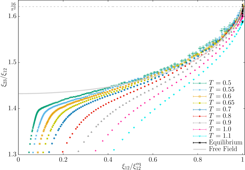
Figure 1: As time evolves [i.e. $\xi_{12}(t_{\mathrm{w}};T)$ grows until it reaches its equilibrium value $\xi_{12}^{\mathrm{eq}}(T)$], the scale-invariant ratio $\xi_{23}(t_{\mathrm{w}},T)/\xi_{12}(t_{\mathrm{w}},T)$ varies, which unveils the dependency on the unknown length-scale $l(t_{\mathrm{w}})$ in Eqs. (11, 12, 15). The figure shows that (barrying small $\xi_{12}^{\mathrm{eq}}(T)$ corrections) the temperature dependence can be absorbed by plotting the data as a function of the scale-invariant ratio $\xi_{12}(t_{\mathrm{w}},T)/\xi_{12}^{\mathrm{eq}}(T)$. Indeed, in agreement with Eq. (15), our data collapse to a master curve when $\xi_{12}^{\mathrm{eq}}(T)$ grows upon lowering the temperature. An analogous master curve can be computed analytically for a non-interacting field (full line), see Eqs. (43) and (45) in A.1. Surprisingly, the master curve for the free-field is a very good approximation for the Edwards-Anderson model. In fact, the free-field prediction might be even exact if the equilibrium limit $\xi_{12}(t_{\mathrm{w}},T)/\xi_{12}^{\mathrm{eq}}(T)\to 1$ is taken first, and the scaling limit $\xi_{12}^{\mathrm{eq}}(T)\to\infty$ is taken afterwards.

Let us now find a workaround on the annoying dependence on $l(t_{\mathrm{w}},T)/\xi_{\mathrm{exp}}(T)$ in Eq. (12) (this dependency is a nuisance because, although $\xi_{\mathrm{exp}}(T)$ can be obtained from our data, see Sect. 4, $l(t_{\mathrm{w}})$ remains a mystery). Fortunately, Eq. (12) suggests that the (computable) dimensionless ratio $\xi_{12}(t_{\mathrm{w}},T)/\xi_{12}^{\mathrm{eq}}(T)$ is a one to one function of $l(t_{\mathrm{w}},T)/\xi_{\mathrm{exp}}(T)$. Hence, we can compare out-equilibrium data at different temperatures by plotting $\xi_{23}/\xi_{12}$ as a function of $\xi_{12}(t_{\mathrm{w}},T)/\xi_{12}^{\mathrm{eq}}(T)$, see Fig. 1. Barring corrections for small $\xi_{12}^{\mathrm{eq}}(T)$ it is clear that the data collapse to a master curve, which is exactly what we expect from Eq. (12). We note as well that the same curve can be computed analytically for the free-field (full curve in Fig. 1). The free-field master curve turns out to be fairly close to the limiting master curve for the Edwards-Anderson model.

We are now ready to address the questions posed at the beginning of this Section.

4 The equilibrium Edwards-Anderson correlations and the theory of a free-field

Let us consider the paramagnetic phase of a typical $D$-dimensional spin system in thermal equilibrium. The asymptotic behaviors of the correlation function are

$$C^{\mathrm{eq}}(r\ll\xi_{\mathrm{exp}})\sim\frac{1}{r^{D-2+\eta}}\,,\quad C^{\mathrm{eq}}(r\gg\xi_{\mathrm{exp}})\sim\xi_{\mathrm{exp}}^{D-2-\eta}\,\frac{K_{Q}(r/\xi_{\mathrm{exp}})}{(r/\xi_{\mathrm{exp}})^{Q}}\,,$$ (16)

where $\eta$ is the anomalous dimension, $Q=(D-2)/2$ and $K_{Q}$ is the $Q$-th order modified Bessel function of the second kind [40]. The normalizations in Eq. (16) ensure that (i) $C^{\mathrm{eq}}(r=1)\sim 1$ [which is certainly the case for the Edwards-Anderson $C_{4}^{\mathrm{eq}}(r;T)$], and (ii) the asymptotic behavior for small and large $r$ connect smoothly at $r=\xi_{\mathrm{exp}}$.

However, let us take seriously for one minute the suggestion that the large-distance asymptotic behavior holds all the way down to $r\sim 1$. Now, specializing to $D=2$ and recalling that $K_{0}(y\to 0)\sim\mathrm{log}\,1/y\,$, we see that the condition $C^{\mathrm{eq}}(r=1)\sim 1$ implies that

$$C^{\mathrm{eq}}_{2D,\mathrm{non-standard}}(r)\sim\frac{K_{0}(r/\xi_{\mathrm{exp}})}{\mathrm{log}\,\xi_{\mathrm{exp}}}\,.$$ (17)

Funnily enough, Fig. 1 suggests that the (equilibrium) 2D Ising spin-glass could really follow the non-standard behavior in Eq. (17), even for $r<\xi_{\mathrm{exp}}$ . Our aim here will be exploring further this hypothesis.

Eq. (17) suggests to start by fitting our equilibrium correlation function to

$$C_{4}^{\mathrm{eq}}(r;T)={\cal A}(\xi_{\mathrm{exp}})\left[\,K_{0}\Big{(}\frac{r}{\xi_{\mathrm{exp}}(T)}\Big{)}\ +\ K_{0}\Big{(}\frac{L-r}{\xi_{\mathrm{exp}}(T)}\Big{)}\,\right]\,,\quad L=512,$$ (18)

where ${\cal A}(\xi_{\mathrm{exp}})$ is an amplitude depending on temperature through $\xi_{\mathrm{exp}}(T)$. We have included in (18) the first-image term, $K_{0}[(L-r)/\xi_{\mathrm{exp}}]$ (mind our periodic boundary conditions), as a further control of finite-size effects. In fact, results turn out to vary by less than a tenth of an error bar (one standard deviation) when the image term is removed. This agreement confirms that the $L=\infty$ limit has been effectively reached.

$T$	$r_{\mathrm{min}}$	$r_{\mathrm{max}}$	$\chi^{2}/\mathrm{dof}$	$A(\xi_{\mathrm{exp}})$	$\xi_{\mathrm{exp}}$	$\xi_{12}^{\mathrm{eq}}/\xi_{\mathrm{exp}}$
0.50	19	202	13.72/182	0.2295 (34)	24.98 (30)	1.5758 (27)
0.55	14	166	70.53/151	0.2469 (27)	18.10 (16)	1.5757 (24)
0.60	10	142	36.85/131	0.2655 (20)	13.63 (8)	1.5771 (21)
0.65	8	113	47.37/104	0.2812 (19)	10.68 (6)	1.5772 (16)
0.70	8	103	62.60/94	0.2981 (20)	8.59 (4)	1.5815 (22)
0.80	5	66	22.82/60	0.3259 (12)	5.942 (17)	1.5798 (9)
0.90	3	50	35.97/46	0.3566 (7)	4.358 (8)	1.5841 (5)
1.00	4	39	5.38/34	0.3867 (10)	3.355 (6)	1.5893 (8)
1.10	4	31	9.70/26	0.4189 (11)	2.671 (4)	1.5994 (9)

Table 1: For each temperature in our simulations, we report the results of a fit to Eq. (18). Given that the numerical estimates of $C_{4}^{\mathrm{eq}}(r;T)$ are dramatically correlated for different distances $r$, we use as fit’s figure of merit, the diagonal $\chi^{2}$ (i.e. the $\chi^{2}$ statistics as computed keeping only the diagonal terms in the covariance matrix). These correlations are responsible for the anomalously low $\chi^{2}$ that we find. The distances included in the fit are $r_{\mathrm{min}}\leq r\leq r_{\mathrm{max}}$ (see Ref. [22] for details). To compute errors in the fit parameters, namely ${\cal A}(\xi_{\mathrm{exp}})$ and $\xi_{\mathrm{exp}}$, we employ the jackknife as implemented in [41]: we fit for each jack-knife block (using for all blocks the diagonal covariance matrix), and compute errors from the blocks fluctuations. We also report the ratio $\xi_{12}^{\mathrm{eq}}/\xi_{\mathrm{exp}}$ (in order to account for statistical correlations, errors were computed with the jackknife). In a free-field theory, $\xi_{12}^{\mathrm{FF},\mathrm{eq}}/\xi_{\mathrm{exp}}=\pi/2=1.5707963\ldots$, see Eq. (42), which is fairly close to our numerical results for the Edwards-Anderson model. The behavior of $\xi_{12}^{\mathrm{eq}}/\xi_{\mathrm{exp}}$ in the limit of large $\xi_{\mathrm{exp}}$ is studied in Fig. 2–bottom.

The results of the fit to Eq. (18) are reported in Table 1. As the reader may check, even in the most difficult case, namely $T=0.5$, $\xi_{\mathrm{exp}}(T)$ is computed with 1% accuracy. We find as well, see Fig. 2–top, that the consistency condition $C^{\mathrm{eq}}(r=1)\sim 1$ expressed in Eq. (17) is well satisfied by our data.

A further confirmation of Eq. (18) comes from the second-moment correlation length. Combining Eq. (9), as applied to $D=2$, with Eq. (42)) we see that Eq. (18) implies

$$\xi^{\mathrm{2nd-moment},\mathrm{eq}}=\xi_{\mathrm{exp}}\,.$$ (19)

Thanks to previous results in Ref. [29], we may compare these two characteristic lengths, see Tables 1 and 2. The agreement is most satisfactory.

$T$	$\xi^{\mathrm{2nd-moment},\mathrm{eq}}$
0.50	23.99(17)
0.55	17.95(11)
0.65	10.753(39)
0.60	13.712(65)
0.70	8.649(26)
0.80	5.968(13)
0.90	4.3854(71)
1.00	3.3657(45)
1.10	2.6782(51)

Table 2: Second moment correlation-lenght in equilibrium as computed in an $L=128$ system by means of a Parallel Tempering simulation (data from Ref. [29]). We expect $\xi^{\mathrm{2nd-moment},\mathrm{eq}}=\xi_{\mathrm{exp}}$, see the discussion of Eq. (19). In fact, letting aside $T=0.5$ (because a $L=128$ lattice is clearly too small to represent the $L\to\infty$ limit for that temperature), the agreeement with the corresponding values for $\xi_{\mathrm{exp}}$ in Table 1 is impressive.

Of course, one cannot expect Eq. (18) to hold for all $r$. Indeed, the fit works only for $r\geq r_{\mathrm{\min}}$, see Table 1. We find that the ratio $r_{\mathrm{\min}}/\xi_{\mathrm{exp}}$ is small, but remains finite as $\xi_{\mathrm{exp}}$ grows upon lowering $T$. In fact, we have empirically found that

$$C_{4}^{\mathrm{eq}}(r;T)-{\cal A}(\xi_{\mathrm{exp}})K_{0}(r/\xi_{\mathrm{exp}})={\cal B}(\xi_{\mathrm{exp}})\frac{\mathrm{exp}[-7r/\xi_{\mathrm{exp}}]}{(r/\xi_{\mathrm{exp}})^{0.2}}\,.$$ (20)

We have checked at $T=0.5$ and $0.55$ that Eq. (20), for which we lack a theoretical justification, works for all $r\geq 1$ (in the sense of an acceptable $\chi^{2}/\mathrm{dof}$). Our standard regularity condition $C^{\mathrm{eq}}_{4}(r=1,T)\sim 1$ tells us that

$${\cal B}(\xi_{\mathrm{exp}})\sim\left[\frac{1}{\xi_{\mathrm{exp}}}\right]^{0.2}\quad\mathrm{for}\quad\xi_{\mathrm{exp}}\to\infty\,.$$ (21)

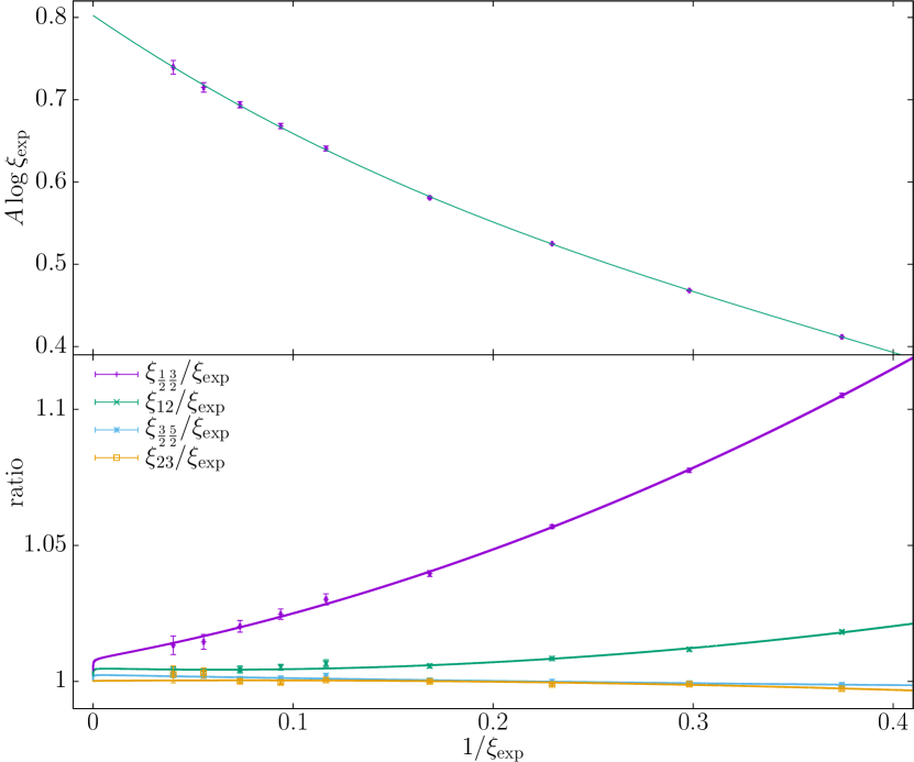
Figure 2: Top: The consistency condition $C^{\mathrm{eq}}(r=1)\sim 1$, see Eq. (17), requires the amplitude in the fit in Eq. (18) to scale as ${\cal A}(\xi_{\mathrm{exp}}\to\infty)\sim 1/\mathrm{log}\,\xi_{\mathrm{exp}}$. Indeed, the plot shows that ${\cal A}(\xi_{\mathrm{exp}})\mathrm{log}\,\xi_{\mathrm{exp}}$ is excellently represented, $\chi^{2}/\mathrm{dof}=2.2/5$, by a cubic polynomial in $1/\xi_{\mathrm{exp}}$, implying ${\cal A}(\xi_{\mathrm{exp}})\mathrm{log}\,\xi_{\mathrm{exp}}\approx 0.8$ for large $\xi_{\mathrm{exp}}$. Bottom: if the non-standard scaling (17) holds true, all the $J_{k}$ defined in Eq. (22) should tend to 1 when $\xi_{\mathrm{exp}}\to\infty$ (the $J_{k}$ are the Edwards-Anderson $\xi^{\mathrm{eq}}_{k,k+1}/\xi_{\mathrm{exp}}$ divided by their free-field counterparts). We show $J_{k}$ as a function of $1/\xi_{\mathrm{exp}}$, for $k=1/2$, $1$,$3/2$ and $2$. Lines are fits to Eq. (24) [note that the function $v(\xi_{\mathrm{exp}})$, Eq. (23), is continuous, but has infinite slope at $\frac{1}{\xi_{\mathrm{exp}}}=0$]. The corresponding figures of merit of these are $\chi^{2}/\mathrm{dof}=2.4/6$ ($k=1/2$), $\chi^{2}/\mathrm{dof}=4.0/6$ ($k=1$), $\chi^{2}/\mathrm{dof}=3.9/6$ ($k=3/2$) and $\chi^{2}/\mathrm{dof}=10.0/6$ ($k=2$).

We are finally ready to consider the extrapolation to large $\xi_{\mathrm{exp}}$ of the ratios $\xi^{\mathrm{eq}}_{k,k+1}/\xi_{\mathrm{exp}}$. We shall start by dividing the $\xi^{\mathrm{eq}}_{k,k+1}/\xi_{\mathrm{exp}}$ by their free-field value in Eq. (42):

$$J_{k}\equiv\frac{\xi^{\mathrm{eq}}_{k,k+1}}{\xi_{\mathrm{exp}}}\,\frac{1}{2}\,\frac{\Gamma^{2}[(k+1)/2]}{\Gamma^{2}[(k+2)/2]}\,.$$ (22)

Our working hypothesis is that $J_{k}\to 1$ for large $\xi_{\mathrm{exp}}$· Then, a straightforward computation starting from Eqs. (20,21) predicts that the finite-$\xi_{\mathrm{exp}}$ corrections for $\xi_{k,k+1}^{\mathrm{eq}}=I_{k+1}^{\mathrm{eq}}/I_{k}^{\mathrm{eq}}$ take the form of a series-expansion in the corrections-to-scaling function

$$v(\xi_{\mathrm{exp}})=\frac{1}{(\xi_{\mathrm{exp}})^{0.2}\,\cal{A}(\xi_{\mathrm{exp}})}\,.$$ (23)

Besides, we have the standard corrections in $1/\xi_{\mathrm{exp}}$, stemming from our considering continuous functions of $r/\xi_{\mathrm{exp}}$ while numerical data can be obtained only for integer $r$. Accordingly, we have fitted our data to

$$J_{k}=1\ +\ a_{k}\,v(\xi_{\mathrm{exp}})\ +\ \frac{b_{k}^{(1)}}{\xi_{\mathrm{exp}}}\ +\ \frac{b_{k}^{(2)}}{\xi^{2}_{\mathrm{exp}}}\,,$$ (24)

with fitting parameters $a_{k}$, $b_{k}^{(1)}$ and $b_{k}^{(2)}$. We have found fair fits to Eq. (24), see Fig. 2–bottom, even for $k$ as small as $k=1/2$ (the smaller the $k$, the more highlighted the small-$r$ region). ${\cal A}(\xi_{\mathrm{exp}}$) is promoted to a continuous function of $\xi_{\mathrm{exp}}$ through the fit in Fig. 2–top [this is needed to compute $v(\xi_{\mathrm{exp}})$]. To assess the relative importance of the correction terms in Eq. (24), we may consider $b_{k}^{(1)}/a_{k}$: in Fig. 2-bottom, these ratios of amplitudes are $b_{1/2}^{(1)}/a_{1/2}\approx 40$, $b_{1}^{(1)}/a_{1}\approx 6.6$, $b_{3/2}^{(1)}/a_{3/2}\approx 11$, and $b_{2}^{(1)}/a_{2}\approx 52$.

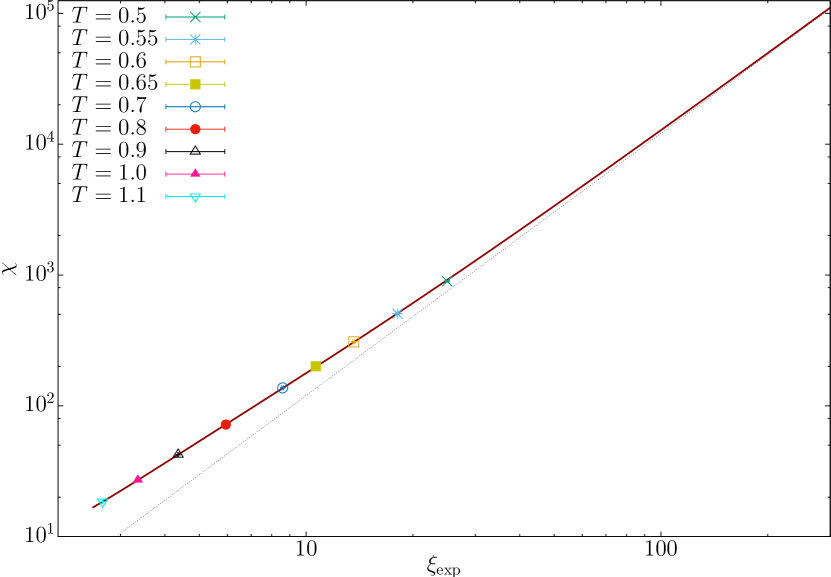
Figure 3: Equilibrium spin glass susceptibility, $\chi=2\pi I_{1}^{\mathrm{eq}}$, see Eq. (10), as a function of $\xi_{\mathrm{exp}}$. The full line is a fit to Eq. (25) ($\chi^{2}/\mathrm{dof}=2.8/5$). One could set $b_{\chi}^{(3)}=0$ in Eq. (25) but at the prize of including only data with $\xi_{\mathrm{exp}}>4$ in the fit (in such a case, one finds $\chi^{2}/\mathrm{dof}=3.6/4$). The dotted line is the dominant term in Eq. (25), $\chi\sim b_{\chi}^{(0)}\xi_{\mathrm{exp}}^{2}$. The horizontal and vertical ranges of the plot have been chosen to match those of Fig. 2 in Ref. [30].

Notice that the equilibrium second-moment correlation length was computed in Ref. [30] [which coincides with $\xi_{\mathrm{exp}}$, see Eq. (19) and Table 2], as well as the spin-glass susceptibility, recall Eq (10). A very large value $\xi_{\mathrm{exp}}\approx 200$ was reached thanks to a combination of Parallel Tempering, cluster methods and Finite-Size Scaling [30]. However, the scaling of $\chi$ was barely under control, in spite of the very large $\xi_{\mathrm{exp}}$. The short-distances behavior identified in Eqs. (20,21) explains this difficulty. Indeed, using the equivalence $\chi=2\pi I_{1}^{\mathrm{eq}}$, only valid in $D=2$, one easily finds that

$$\chi=\xi^{2}\Big{[}b_{\chi}^{0}\ +a_{\chi}\,v(\xi_{\mathrm{exp}})\ +\ \frac{b_{\chi}^{(1)}}{\xi_{\mathrm{exp}}}\ +\ \frac{b_{\chi}^{(2)}}{\xi^{2}_{\mathrm{exp}}}\ +\ \frac{b_{\chi}^{(3)}}{\xi^{3}_{\mathrm{exp}}}\ +\ \ldots\ \Big{]}\,,$$ (25)

where $a_{\chi}$ and the $b_{\chi}^{(i)}$ are scaling amplitudes. A fair fit to Eq. (25) is shown in the full line in Fig. 3. The width of that full line has been chosen to correspond with the error bars, while the dotted line in Fig. 3 is the leading term $\chi\sim b_{\chi}^{(0)}\xi_{\mathrm{exp}}^{2}$. We see in Fig. 3 that the full and the dotted lines coalesce only for $\xi_{\mathrm{exp}}>100$, in nice agreement with the results found in Ref. [30].

In summary, in the scaling limit $\xi_{\mathrm{eq}}\to\infty$, the equilibrium correlation-function for the Ising spin glass seems to follow the non-standard scaling in Eq. (17). However, some readers may consider far-fetched our parameterization of short-distances corrections to the free-field propagator in Eqs. (20) and  (21). These skeptical readers may keep the more conservative conclusion that violations to the free-field prediction $J_{k}(\xi_{\mathrm{eq}}\to\infty)=1$ are, at most, of 0.3% for $k=1/2,1,3/2$, and $2$.

5 The out-equilibrium Edwards-Anderson correlations and the theory of a free-field

Relating the Langevin dynamics of a free-field with the spin-glass dynamics may seem surprising at first sight. Indeed, the dynamics of a spin-glass in its paramagnetic phase may be characterized through a scaling function [22]

$$\frac{\xi_{12}(t_{\mathrm{w}},T)}{\xi_{12}^{\mathrm{eq}}(T)}={\cal F}\left(\frac{t_{w}}{\tau(T)}\right)\ +\ {\cal O}\Big{(}\,[\xi_{12}(t_{\mathrm{w}},T)]^{-\omega},[\xi_{12}^{\mathrm{eq}}(T)]^{-\omega}\,\Big{)}\,,$$ (26)

where exponent $\omega$ controls corrections to scaling, $\tau(T)$ is a characteristic time scale, and the dynamics at short times is described by a dynamic exponent $\hat{z}$:

$${\cal F}(x\to 0)\propto x^{1/\hat{z}}\,\,.$$ (27)

We have found empirically $\hat{z}\approx 7$ for the Edwards-Anderson model [22].

The analogous exponent for the free-field is $\hat{z}_{\mathrm{FF}}=2$ (A.1). The obvious, hardly surprising conclusion is that spin-glass dynamics is enormously slower than free-field dynamics. However, one may synchronize clocks between these two wildly differing systems by requiring (superscripts FF stand for free field)

$$f=\frac{\xi_{12}(t_{\mathrm{w}},T)}{\xi_{12}^{\mathrm{eq}}(T)}=\frac{\xi^{\mathrm{FF}}_{12}(t_{\mathrm{w}}^{\mathrm{FF}})}{\xi_{12}^{\mathrm{FF},\mathrm{eq}}}\,.$$ (28)

This clock synchronization was implicitly performed in Fig. 1. We zoom this figure in Fig. 4 making it clear that the clock-synchronization works only approximately: the free-field and the Edwards-Anderson limit behaves in the same way only in the limit of a system in thermal equilibrium.

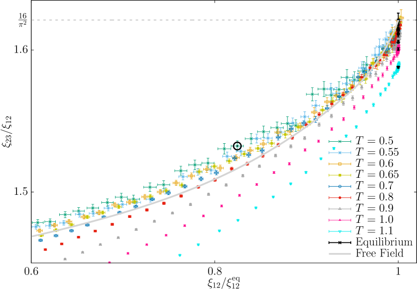
Figure 4: Zoom of data in Fig. 1. The scaling limit $\xi_{\mathrm{exp}}(T)\to\infty$ at fixed $\xi_{12}(t_{\mathrm{w}},T)/\xi_{12}^{\mathrm{eq}}(T)$ slightly differs for the Edwards-Anderson model (data points) and for the non-interacting field (full line). However, disentangling the two-models behavior becomes difficult upon approaching equilibrium, $\xi_{12}(t_{\mathrm{w}},T)/\xi_{12}^{\mathrm{eq}}(T)\to 1$. The time $t_{\mathrm{w}}$ which is explicitly compared with the free-field model in Fig. 5 is marked by a circle (for $T=0.5$).

In order to further expose the difference, in Fig. 5 we compare the Edwards-Anderson model correlation function $C_{4}(r,t_{\mathrm{w}};T)$ with its free-field counterpart in Fig. 5, after the appropriate parameter matching. It is clear that, even setting the same $\xi_{\mathrm{exp}}$ for both models and synchronizing the clocks as in Eq. (28), the free-field propagator has a higher curvature, as a function of $r$.

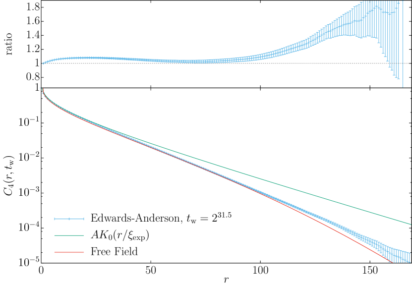
Figure 5: Main: For $T=0.5$, we compare the Edwards-Anderson correlation function $C_{4}(r,t_{\mathrm{w}})$ with its free-field counterpart $G(r,t_{\mathrm{w}}^{\mathrm{FF}})$, see Eq. (31). To match the parameters for the free-field, we fix $\xi^{\mathrm{FF}}_{12}(t_{\mathrm{w}}^{\mathrm{FF}})/\xi_{12}^{\mathrm{FF},\mathrm{eq}}=0.824585$, the value pinpointed by the circle in Fig. 4, and take $\xi_{\mathrm{exp}}(T=0.5)$ from Table 1. The overall normalization of the free-field is chosen to have $C_{4}(r=1,t_{\mathrm{w}})=G(r=1,t_{\mathrm{w}}^{\mathrm{FF}})$. We also compare the two propagators with the asymptotic form of the equilibrium Edwards-Anderson correlation function, ${\cal A}(\xi_{\mathrm{exp}})K_{0}(r/\xi_{\mathrm{exp}})$. Top: ratio $C_{4}(r,t_{\mathrm{w}})/G(r,t_{\mathrm{w}}^{\mathrm{FF}})$ as a function of $r$.

6 Conclusions

We have studied the out-of-equilibrium dynamics of the two dimensional Edwards-Anderson model with binary couplings. We have been able to study the full range of the dynamics: from the initial transients to the equilibrium through numerical simulations with a time span of 11 orders of magnitude. We have considered the spatial dependence of the Edwards-Anderson correlation function $C_{4}(r,t_{\mathrm{w}})$, that has been compared with the propagator of a free-field theory. Much to our surprise, we found that, after an appropriate clock synchronization between the two models, the free-field propagator provides a very good approximation to $C_{4}(r,t_{\mathrm{w}})$ in the out-equilibrium regime. Furthermore, in the scaling limit $\xi_{12}^{\mathrm{eq}}$ for the equilibrium regime, after a logarithmic wavefunction renormalization, we find extremely difficult to distinguish the two models numerically.

7 Acknowledgments

We thank Prof. Gabriel Álvarez for discussions. This project has received funding from the European Research Council (ERC) under the European Union’s Horizon 2020 research and innovation program (grant agreement No 694925). We were partially supported by MINECO (Spain) through Grant Nos. FIS2015-65078-C2, FIS2016-76359-P, by the Junta de Extremadura (Spain) through Grant No. GRU10158, GR18079 and IB16013 (these five contracts were partially funded by FEDER). Our simulations were carried out at the BIFI supercomputing center (using the Memento and Cierzo clusters) and at ICCAEx supercomputer center in Badajoz (Grinfishpc and Iccaexhpc). We thank the staff at BIFI and ICCAEx supercomputing centers for their assistance.

Appendix A The out-equilibrium dynamics of the free scalar field

The Edwards-Anderson model in spatial dimension $D=2$ lies within its paramagnetic phase at all positive temperatures. Therefore, the relevant Renormalization-Group fixed point is the one of the free scalar-field (see e.g. [27, 28]). This observation implies that, at least in equilibrium, the free-field fixed point rules the system behavior at distances $r\gg\xi_{\mathrm{eq}}$.

However, the $D=2$ Edwards-Anderson model and the free-field theory might differ for distances $r\sim\xi_{\mathrm{eq}}$. Futhermore, at these length-scales, the two theories should be compared both under equilibrium and out-equilibrium conditions. In order to confront the two models, we compute here for the free-field the same quantities that were studied for the Edwards-Anderson model in the main text.

Our starting point is the Langeving dynamics for a free field [27]. At the initial time, the field is fully disordered. The two-body correlation function $G(\mathitbf{r},t_{\mathrm{w}})$ is the analogous in the free-field theory of the Edwards-Anderson correlation function $C_{4}(\mathitbf{r},t_{\mathrm{w}})$, recall Eq. (3). We can compute explictly the free-field $G$ in Fourier space

$$\hat{G}(\mathitbf{p},t_{\mathrm{w}})=\frac{\big{(}1-\exp[-2t_{\mathrm{w}}(p^{2}+\xi_{\mathrm{exp}}^{-2})]\big{)}}{p^{2}+\xi_{\mathrm{exp}}^{-2}}\,.$$ (29)

The above expression defines the so-called exponential correlation length, $\xi_{\mathrm{exp}}$ (indeed, $\hat{G}(\mathitbf{p},t_{\mathrm{w}})$ tends to the Gaussian propagator $1/(p^{2}+\xi_{\mathrm{exp}}^{-2})$ in the limit of large $t_{\mathrm{w}}$). Note as well that there are two characteristic lengths in Eq. (29), namely the correlation length $\xi_{\mathrm{exp}}$ and the diffusion length $\sqrt{t_{\mathrm{w}}}$. Thus, before starting our computation, it will be useful to introduce dimensionless length ($\mathitbf{y}$) and time variables ($w$):

$$\mathitbf{y}=\mathitbf{r}/\xi_{\mathrm{exp}}\,,\quad w=2t_{\mathrm{w}}/\xi_{\mathrm{exp}}^{2}\,.$$ (30)

Rotational-invariance implies that the propagator will depend only on the length $y$ of vector $\mathitbf{y}$ (on a lattice, rotational invariance is recovered only in the continuum limit $\xi_{\mathrm{exp}}\to\infty$ [27]; in the context of out-equilibrium spin glasses, the recovery of rotational invariance was investigated in [16]).

A straightforward computation (A.3) allows us to transform back Eq. (29) from Fourier to real space:

$$G(\mathitbf{r},t_{\mathrm{w}})=\xi_{\mathrm{exp}}^{2-D}\,F_{D}(y,w)\,,\ F_{D}(y,w)=\frac{1}{(4\pi)^{D/2}}\int_{0}^{w}\mathrm{d}s\,\frac{\mathrm{exp}[-s-\frac{y^{2}}{4s}]}{s^{D/2}}\,.$$ (31)

Armed with Eq. (31) we can compute (the free-field analogous of) the $I_{k}(t_{\mathrm{w}})$ integrals defined in Eq. (5). This computation is performed in A.1. Eq. (31) makes it simple as well the discussion of the large $y$ limit taken at fixed $w$ (A.2).

The opposite limit, $w\to\infty$ for fixed $y$, yields the (equilibrium) Gaussian propagator (see [27] for further details):

$$G^{\mathrm{eq}}(\mathitbf{r})=\frac{\xi_{\mathrm{exp}}^{2-D}}{(4\pi)^{D/2}}\int_{0}^{\infty}\,\mathrm{d}s\,\frac{\mathrm{exp}[-s-\frac{y^{2}}{4s}]}{s^{D/2}}=\frac{\xi_{\mathrm{exp}}^{2-D}}{(2\pi)^{D/2}}\frac{K_{Q}(y)}{y^{Q}}\,,$$ (32)

where $Q=(D-2)/2$ and $K_{Q}$ is the $Q$-th order modified Bessel function of the second kind [40]. The large and small-$y$ behavior for $D>2$ are

$$G^{\mathrm{eq}}(\mathitbf{r}/\xi_{\mathrm{exp}}\to\infty)\sim\frac{\mathrm{e}^{-y}}{y^{(D-1)/2}}\,,\quad G^{\mathrm{eq}}(\mathitbf{r}/\xi_{\mathrm{exp}}\to 0)\sim\frac{1}{y^{D-2}}\,.$$ (33)

The neighborhood of $y\to 0$ for the case $D=2$ deserves special care:

$$G^{\mathrm{eq}}(\mathitbf{r}/\xi_{\mathrm{exp}}\to 0)\sim\mathrm{log}\frac{1}{y}\,.$$ (34)

A.1 Integral estimators of dynamic correlations

In analogy with Eq. (5), we shall characterize the free-field propagator through its moments (the superindex $\mathrm{FF}$ stands for free field)

$$I^{\mathrm{FF}}_{k}(t_{\mathrm{w}})=\int_{0}^{\infty}\mathrm{d}r\,r^{k}\,G(r,t_{\mathrm{w}})\,,$$ (35)

where we have exploited the isotropy of the free-field propagator. We shall specialize to $D=2$, and compute the moments for a propagator of the form

$$G(r,t_{\mathrm{w}})={\cal A}\int_{0}^{w}\,\mathrm{d}s\,\frac{\mathrm{exp}[-s-\frac{y^{2}}{4s}]}{s}\,,$$ (36)

recall Eqs. (30,31). In particular, Eq. (31) implies for the amplitude ${\cal A}=1/(4\pi)$. However, the main results in this section will be ${\cal A}$-independent (in particular, ${\cal A}$ could depend on $\xi_{\mathrm{exp}}$ or $w$). We find

$$I^{\mathrm{FF}}_{k}(t_{\mathrm{w}}) = {\cal A}\,\xi_{\mathrm{exp}}^{k+1}\,\int_{0}^{\infty}\mathrm{d}y\,y^{k}\int_{0}^{w}\,\mathrm{d}s\,\frac{\mathrm{exp}[-s-\frac{y^{2}}{4s}]}{s}\,,$$ (37)

$$= {\cal A}\,\xi_{\mathrm{exp}}^{k+1}\,2^{k}\,\Gamma[(k+1)/2]\,\gamma[(k+1)/2,w]\,,$$ (38)

by interchanging the ordering of the $y$ and $s$ integrals. In the above expression, $\Gamma(x)$ is Euler’s Gamma function and $\gamma(x,w)$ is the lower incomplete Gamma function

$$\gamma(x,w)=\int_{0}^{w}\mathrm{d}s\,s^{x-1}\mathrm{e}^{-s}\,,\quad\gamma(x,w\to\infty)=\Gamma(x)+{\cal O}(w^{x-1}\mathrm{e}^{-w})\,.$$ (39)

For later use, we recall its small-$w$ behavior:

$$\gamma(x,w\to 0)=\frac{w^{x}}{x}+{\cal O}(w^{x+1})\,,\quad$$ (40)

The $\xi^{\mathrm{FF}}_{k,k+1}(t_{\mathrm{w}})$ estimate of the size of the coherence length, recall Eq. (4), is

$$\xi^{\mathrm{FF}}_{k,k+1}(t_{\mathrm{w}})\equiv\frac{I^{\mathrm{FF}}_{k+1}(t_{\mathrm{w}})}{I^{\mathrm{FF}}_{k}(t_{\mathrm{w}})}=2\,\frac{\Gamma[(k+2)/2]}{\Gamma[(k+1)/2]}\,\frac{\gamma[(k+2)/2,w]}{\gamma[(k+1)/2,w]}\,\xi_{\mathrm{exp}}\,.$$ (41)

The equilibrium limit, $w\to\infty$, is approached exponentially in $w$ [Eq. (39)]:

$$\xi^{\mathrm{FF},\mathrm{eq}}_{k,k+1}=2\,\frac{\Gamma^{2}[(k+2)/2]}{\Gamma^{2}[(k+1)/2]}\,\xi_{\mathrm{exp}}\,.$$ (42)

In other words, the integral estimators of the coherence-length, in equilibrium but also out-equilibrium (at fixed $w$), are proportional to the exponential correlation length $\xi_{\mathrm{exp}}$.

In the main text, we payed a major attention to the approach to equilibrium of $\xi_{12}$ as computed in the Edwards-Anderson model. The free-field analogous of Eq. (26) is

$$\frac{\xi^{\mathrm{FF}}_{12}(t_{\mathrm{w}})}{\xi_{12}^{\mathrm{FF},\mathrm{eq}}}=\frac{\gamma(3/2,w)}{\Gamma(3/2)}\frac{\Gamma(1)}{\gamma(1,w)}\,.$$ (43)

It is remarkable that Eq. (43) conforms exactly to the ansatz expressed for the Edwards-Anderson model in Eq. (26). Furthermore, because $w=2t_{\mathrm{w}}/\xi^{2}_{\mathrm{exp}}(T)$, we find $\tau_{\mathrm{FF}}(T)=\xi^{2}_{\mathrm{exp}}(T)/2$ for the free-field analogous of the time scale in Eq. (26).

We can also compute the free-field exponent $\hat{z}_{\mathrm{FF}}$, recall Eq. (27), from the small-$w$ expansion of Eq. (43) [recall Eq. (40)]:

$$\frac{\xi^{\mathrm{FF}}_{12}(t_{\mathrm{w}})}{\xi_{12}^{\mathrm{FF},\mathrm{eq}}}=\frac{2\sqrt{\pi}}{3}w^{1/2}+{\cal O}(w^{3/2})\,,$$ (44)

which implies for the free-field $\hat{z}_{\mathrm{FF}}=2$. The reader may check from Eqs. (40,41,42) that the small-$w$ behavior is $\xi^{\mathrm{FF}}_{k,k+1}(t_{\mathrm{w}})/\xi^{\mathrm{FF},\mathrm{eq}}_{k,k+1}\sim\sqrt{w}$ for any $k$, hence the result $\hat{z}_{\mathrm{FF}}=2$ is $k$-independent. Because $\hat{z}_{\mathrm{FF}}=2$ is rather smaller than the $\hat{z}\approx 7$ value that we found numerically for the Edwards-Anderson model, we conclude that the dynamics for the Edwards-Anderson is enormously slower than the free-field Langevin dynamics, which is hardly surprising.

Nevertheless, Eq. (43) shows that $\xi^{\mathrm{FF}}_{12}(t_{\mathrm{w}})/\xi_{12}^{\mathrm{FF},\mathrm{eq}}$ is a monotonously increasing function of $w$. Hence, one can parameterize the free-field dynamics in terms of $\xi^{\mathrm{FF}}_{12}(t_{\mathrm{w}})/\xi_{12}^{\mathrm{FF},\mathrm{eq}}$, rather than $w$. In this way, we can obtain a meaningful comparison of the free-field with the Edwards-Anderson dynamics. The quantities compared are dimensionless ratios such as $\xi_{k,k+1}(t_{\mathrm{w}})/\xi_{\mathrm{exp}}$ [its value for the free-field is given in Eq. (41)], or in terms of ratios not involving $\xi_{\mathrm{exp}}$ such as $\xi_{23}(t_{\mathrm{w}})/\xi_{12}(t_{\mathrm{w}})$, recall Figs. 1. From Eq. (41), we easily find

$$\frac{\xi^{\mathrm{FF}}_{23}(t_{\mathrm{w}})}{\xi^{\mathrm{FF}}_{12}(t_{\mathrm{w}})}=\frac{4}{\pi}\frac{\gamma(2,w)\gamma(1,w)}{\gamma^{2}(3/2,w)}\,.$$ (45)

The limiting values are $\xi^{\mathrm{FF}}_{23}/\xi^{\mathrm{FF}}_{12}=9/(2\pi)$ (for $w\to 0$), and $\xi^{\mathrm{FF}}_{23}/\xi^{\mathrm{FF}}_{12}=16/\pi^{2}$ (for $w\to\infty$).

A.2 Asymptotic behavior of $F_{D}(y,w)$ (large $y$ at fixed $w$)

For any finite fixed-time $t_{\mathrm{w}}$, the free-field propagator in Fourier space, $\hat{G}(\mathitbf{p},t_{\mathrm{w}})$ see Eq. (29), is an analytic function in the whole complex-plane of the variable $p^{2}$. It follows that the function $F_{D}(y,w)$, defined in Eq. (31), tends to zero at large $y$ faster than $\mathrm{e}^{-Ay}$ for any $A>0$ (a simply exponential decay corresponds with a pole singularity at $p^{2}=-A^{2}$ [27]). This statement is in apparent contradiction with the asymptotic behavior in Eq. (33) which is exact, but only for $t_{\mathrm{w}}=\infty$. The way out of the paradox is simple: $\hat{G}(p^{2}=-\xi_{\mathrm{exp}}^{2},t_{\mathrm{w}})=2t_{\mathrm{w}}$ which becomes a pole singularity only in the $t_{\mathrm{w}}\to\infty$ limit. It is clear that, at finite $t_{\mathrm{w}}$, some sort of crossover phenomenon is present. In this section we aim to discuss this crossover.

We start from the integral representation (31)

$$F_{D}(y,w) = \frac{1}{(4\pi)^{D/2}}\int_{0}^{w}\,\mathrm{d}s\,\mathrm{e}^{\Psi_{D}(s,y)}\,,$$ (46)

$$\Psi_{D}(s,y) = -\frac{y^{2}}{4s}\,-s\,-\frac{D}{2}\,\mathrm{log}\,s\,.$$ (47)

Consider the function $\Psi_{D}(s,y)$ at fixed $y$. $\Psi_{D}(s,y)$ tends to $-\infty$ both for $s\to 0,\infty$. These two asymptotic behaviors of $\Psi_{D}(s,y)$ are separated by a maximum at

$$s^{*}(y)=\frac{y^{2}}{D+\sqrt{D^{2}+4y^{2}}}\,.$$ (48)

Note that $s^{*}(y\to 0)\sim y^{2}$, but $s^{*}(y\to\infty)\sim y/2$.

Now, imagine that we hold $y$ fixed ($y$ should be large enough to have $s^{*}(y)\approx y/2$ to a good approximation). If $w\gg s^{*}(y)$ we can estimate $F_{D}(y,w)$ through a straightforward saddle-point expansion around $s^{*}(y)$ that reproduces the $w=\infty$ asymptotic behavior in Eq. (33):

$$F^{(\mathrm{SP})}_{D}(y,w)\sim\frac{\mathrm{e}^{-y}}{y^{(D-1)/2}}\,.$$ (49)

The error induced by the finite $w$ is $\sim\mathrm{e}^{\Psi_{D}(w,y)}/|\partial_{w}\Psi_{D}(w,y)|$, hence exponentially small.

However, because $s^{*}(y)\approx y/2$ for large $y$, upon increasing $y$ the saddle point $s^{*}(y)$ eventually exits the integration interval $0<s<w$ (i.e. for $y\gtrsim 2w$ we have $s^{*}(y)>w$). Obviously, the saddle-point expansion becomes inaccurate for such a large $y$. Under such circumstances, the integrand in Eq. (46) is maximal at $s=w$, which gives the large-$y$ expansion

$$F^{(\mathrm{Extreme})}_{D}(y,w)\sim\frac{\mathrm{e}^{\Psi_{D}(y,w)}}{|\partial_{w}\Psi_{D}(w,y)|}=\frac{\mathrm{exp}[-w-\frac{y^{2}}{4w}]}{w^{D/2}}\frac{4w^{2}}{y^{2}-2Dw-4w^{2}}\,.$$ (50)

In summary, for any (dimensionless) time variable $w$ one may identify a (dimensionless) crossover length $l_{\mathrm{co}}$ through $s^{*}(l_{\mathrm{co}})=w$. If $y\ll l_{\mathrm{co}}$ then $F_{D}(y,w)$ is given to an excellent accuracy by its equilibrium limit, Eq. (32). Instead, for $y\gg l_{\mathrm{co}}$ the asymptotic behavior is given by Eq. (50). Eq. (48) provides asymptotic estimates for the cross-over length,

$$l_{\mathrm{co}}(w\to\infty)\sim 2w\,,\quad\mathrm{and}\quad l_{\mathrm{co}}(w\to 0)\sim\sqrt{2Dw}\,.$$ (51)

A.3 Back to real space: the computation of $F_{D}(y,z)$

For the sake of completeness, let us sketch the derivation of Eq. (31). We need to perform the inverse Fourier-transform:

$$G(\mathitbf{r},t_{\mathrm{w}})=\int\frac{\mathrm{d}^{D}\mathitbf{p}}{(2\pi)^{D}}\,\mathrm{e}^{\mathrm{i}\mathitbf{p}\cdot\mathitbf{r}}\,\frac{\big{(}1-\exp[-2t_{\mathrm{w}}(p^{2}+\xi_{\mathrm{exp}}^{-2})]\big{)}}{p^{2}+\xi_{\mathrm{exp}}^{-2}}\,.$$ (52)

After introducing the (dimensionless) length and time variables $y$ and $w$, recall Eq. (30), as well as the dimensionless momentum $\mathitbf{u}\equiv\mathitbf{p}\,\xi_{\mathrm{exp}}$, we find

$$G(\mathitbf{r},t_{\mathrm{w}})=\xi_{\mathrm{exp}}^{2-D}F_{D}(y,w)\,,\ F_{D}(y,w)=\int\frac{\mathrm{d}^{D}\mathitbf{u}}{(2\pi)^{D}}\,\mathrm{e}^{\mathrm{i}\mathitbf{u}\cdot\mathitbf{y}}\frac{1-\mathrm{e}^{-w(u^{2}+1)}}{u^{2}+1}\,.$$ (53)

Next, we note that the derivative with respect to $w$ of $F_{D}(y,w)$ can be computed by derivating under the integral sign (we are left with a Gaussian integral):

$$\partial_{w}F_{D}(y,w)=\int\frac{\mathrm{d}^{D}\mathitbf{u}}{(2\pi)^{D}}\,\mathrm{e}^{\mathrm{i}\mathitbf{u}\cdot\mathitbf{y}}\mathrm{e}^{-w(u^{2}+1)}=\frac{1}{(4\pi)^{D/2}}\frac{\mathrm{exp}[-w-\frac{y^{2}}{4w}]}{w^{D/2}}\,.$$ (54)

Finally, because $F_{D}(y,w=0)=0$, Eq. (31) is recovered from

$$F_{D}(y,w)=F_{D}(y,w)-F_{D}(y,w=0)=\int_{0}^{w}\mathrm{d}s\,\partial_{s}F_{D}(y,s)\,.$$ (55)

References

References

- [1] Ballesteros H G, Cruz A, Fernandez L A, Martín-Mayor V, Pech J, Ruiz-Lorenzo J J, Tarancon A, Tellez P, Ullod C L and Ungil C 2000 Phys. Rev. B 62 14237–14245
- [2] Palassini M and Caracciolo S 1999 Phys. Rev. Lett. 82 5128–5131
- [3] Fisher D S and Huse D A 1988 Phys. Rev. B 38(1) 373–385
- [4] Rieger H, Steckemetz B and Schreckenberg M 1994 EPL (Europhysics Letters) 27 485
- [5] Marinari E, Parisi G, Ruiz-Lorenzo J and Ritort F 1996 Phys. Rev. Lett. 76(5) 843–846
- [6] Kisker J, Santen L, Schreckenberg M and Rieger H 1996 Phys. Rev. B 53(10) 6418–6428
- [7] Joh Y G, Orbach R, Wood G G, Hammann J and Vincent E 1999 Phys. Rev. Lett. 82(2) 438–441
- [8] Berthier L and Bouchaud J P 2002 Phys. Rev. B 66(5) 054404
- [9] Jönsson P E, Yoshino H, Nordblad P, Aruga Katori H and Ito A 2002 Phys. Rev. Lett. 88(25) 257204
- [10] Berthier L and Young A P 2004 Phys. Rev. B 69(18) 184423
- [11] Jiménez S, Martín-Mayor V and Pérez-Gaviro S 2005 Phys. Rev. B 72(5) 054417
- [12] Berthier L and Young A P 2005 Phys. Rev. B 71(21) 214429
- [13] Jaubert L C, Chamon C, Cugliandolo L F and Picco M 2007 J. Stat. Mech. 2007 P05001
- [14] Belletti F, Cotallo M, Cruz A, Fernandez L A, Gordillo-Guerrero A, Guidetti M, Maiorano A, Mantovani F, Marinari E, Martín-Mayor V, Sudupe A M, Navarro D, Parisi G, Perez-Gaviro S, Ruiz-Lorenzo J J, Schifano S F, Sciretti D, Tarancon A, Tripiccione R, Velasco J L and Yllanes D (Janus Collaboration) 2008 Phys. Rev. Lett. 101 157201
- [15] Aron C, Chamon C, Cugliandolo L F and Picco M 2008 Journal of Statistical Mechanics: Theory and Experiment 2008 P05016
- [16] Belletti F, Cruz A, Fernandez L A, Gordillo-Guerrero A, Guidetti M, Maiorano A, Mantovani F, Marinari E, Martín-Mayor V, Monforte J, Muñoz Sudupe A, Navarro D, Parisi G, Perez-Gaviro S, Ruiz-Lorenzo J J, Schifano S F, Sciretti D, Tarancon A, Tripiccione R and Yllanes D (Janus Collaboration) 2009 J. Stat. Phys. 135 1121
- [17] Guchhait S and Orbach R 2014 Phys. Rev. Lett. 112(12) 126401
- [18] Manssen M and Hartmann A K 2015 Phys. Rev. B 91(17) 174433
- [19] Baity-Jesi M, Calore E, Cruz A, Fernandez L A, Gil-Narvión J M, Gordillo-Guerrero A, Iñiguez D, Maiorano A, Marinari E, Martin-Mayor V, Monforte-Garcia J, Muñoz Sudupe A, Navarro D, Parisi G, Perez-Gaviro S, Ricci-Tersenghi F, Ruiz-Lorenzo J J, Schifano S F, Seoane B, Tarancón A, Tripiccione R and Yllanes D 2017 Proceedings of the National Academy of Sciences 114 1838–1843
- [20] Baity-Jesi M, Calore E, Cruz A, Fernandez L A, Gil-Narvion J M, Gordillo-Guerrero A, Iñiguez D, Maiorano A, Marinari E, Martin-Mayor V, Monforte-Garcia J, Muñoz Sudupe A, Navarro D, Parisi G, Perez-Gaviro S, Ricci-Tersenghi F, Ruiz-Lorenzo J J, Schifano S F, Seoane B, Tarancon A, Tripiccione R and Yllanes D (Janus Collaboration) 2017 Phys. Rev. Lett. 118(15) 157202
- [21] Guchhait S and Orbach R L 2017 Phys. Rev. Lett. 118 157203
- [22] Fernández L A, Marinari E, Martín-Mayor V, Parisi G and Ruiz-Lorenzo J 2018 An experiment-oriented analysis of 2d spin-glass dynamics: a twelve time-decades scaling study (Preprint arXiv:1805.06738)
- [23] Boettcher S 2005 Phys. Rev. Lett. 95 197205
- [24] Guchhait S, Kenning G G, Orbach R L and Rodriguez G F 2015 Phys. Rev. B 91(1) 014434
- [25] Guchhait S and Orbach R L 2015 Phys. Rev. B 92(21) 214418
- [26] Zhai Q, Harrison D C, Tennant D, Dalhberg E D, Kenning G G and Orbach R L 2017 Phys. Rev. B 95(5) 054304
- [27] Parisi G 1988 Statistical Field Theory (Addison-Wesley)
- [28] Amit D J and Martín-Mayor V 2005 Field Theory, the Renormalization Group and Critical Phenomena 3rd ed (Singapore: World Scientific)
- [29] Fernandez L A, Marinari E, Martin-Mayor V, Parisi G and Ruiz-Lorenzo J J 2016 Phys. Rev. B 94(2) 024402
- [30] Jörg T, Lukic J, Marinari E and Martin O C 2006 Phys. Rev. Lett. 96(23) 237205
- [31] Edwards S F and Anderson P W 1975 Journal of Physics F: Metal Physics F 5 965
- [32] Edwards S F and Anderson P W 1976 J. Phys. F 6 1927
- [33] Parisi G 1994 Field Theory, Disorder and Simulations (World Scientific)
- [34] Mydosh J A 1993 Spin Glasses: an Experimental Introduction (London: Taylor and Francis)
- [35] Belletti F, Cotallo M, Cruz A, Fernandez L A, Gordillo A, Maiorano A, Mantovani F, Marinari E, Martín-Mayor V, Muñoz Sudupe A, Navarro D, Perez-Gaviro S, Ruiz-Lorenzo J J, Schifano S F, Sciretti D, Tarancon A, Tripiccione R and Velasco J L (Janus Collaboration) 2008 Comp. Phys. Comm. 178 208–216
- [36] Khoshbakht H and Weigel M 2017 Domain-wall excitations in the two-dimensional Ising spin glass Phys. Rev. B 97 064410
- [37] Katzgraber H W , Lee L W and Young A P 2004 Phys. Rev. B 70 014417
- [38] Cooper F, Freedman B and Preston D 1982 Nucl. Phys. B 210 210
- [39] Caracciolo S, Edwards R G, Pelissetto A and Sokal A D 1993 Nuclear Physics B 403 475 – 541
- [40] Olver F W J, Lozier D W, Boisvert R and Clark C (editors) 2010 NIST Handbook of Mathematical Functions (Cambridge: Cambridge University Press) URL http://dlmf.nist.gov/
- [41] Yllanes D 2011 Rugged Free-Energy Landscapes in Disordered Spin Systems Ph.D. thesis Universidad Complutense de Madrid (Preprint arXiv:1111.0266)