Improved Person Detection on Omnidirectional Images with Non-maxima Suppression

Abstract

We propose a person detector on omnidirectional images, an accurate method to generate minimal enclosing rectangles of persons. The basic idea is to adapt the qualitative detection performance of a convolutional neural network based method, namely YOLOv2 to fish-eye images. The design of our approach picks up the idea of a state-of-the-art object detector and highly overlapping areas of images with their regions of interests. This overlap reduces the number of false negatives. Based on the raw bounding boxes of the detector we fine-tuned overlapping bounding boxes by three approaches: non-maximum suppression, soft non-maximum suppression and soft non-maximum suppression with Gaussian smoothing. The evaluation was done on the PIROPO database and an own annotated Flat dataset, supplemented with bounding boxes on omnidirectional images. We achieve an average precision of 64.4 % with YOLOv2 for the class person on PIROPO and 77.6 % on Flat. For this purpose we fine-tuned the soft non-maximum suppression with Gaussian smoothing.

1 Introduction

Convolutional neural networks (CNNs) were treaded for several tasks in computer vision in the recent years. Finding objects in images (i.e. object detection) belongs to these tasks. A main requirement for the detection of objects in images for current CNNs are accurate real-world training data. In this paper we propose a method to detect objects in fish-eye images of indoor scenes using a state-of-the-art object detector.

The object detection in indoor scenes with a limited number of image sensors can be reached with images from omnidirectional cameras. These cameras are suited for capturing one room with a single sensor due to a field of view of about $180\mathrm{°}$. Our goal is to detect objects in indoor scenes in omnidirectional data with a detector trained on perspective images.

Beside our application, the field of active assisted living, the detection of objects in omnidirectional image data can be used in mobile robots and in the field of autonomous driving.

The remainder of this paper is structured as follows: Section 2 presents previous research activities in object detection. Section 3 illustrates the working principle of a neural network based object detector. Section 4 explains how our virtual cameras are generated. Section 5 shows the theoretical background for different variants of non-maximum suppression (NMS). Section 6 describes our experiments for the generation of bounding boxes and the evaluation of our results on common error metrics. Section 7 summarizes the paper’s content, concludes our observations and gives ideas for future work. The results of our work, the image data and the evaluation of the results, can be found at https://gitlab.com/auxilia/omnidetector.

2 Related work

State-of-the-art object detectors predict bounding boxes on perspective images over several classes. A region-based, fully connected convolutional network for accurate and efficient object detection is R-FCN [Dai et al., 2016]. As a standard practice, the results of the detector based on ResNet-101 architecture [He et al., 2016] are post-processed with non-maximum suppression (NMS) using a threshold of 0.3 to the intersection over union (IoU) [Girshick et al., 2013]. The single shot multi-box detector (SSD) by [Liu et al., 2016] provides an improvement of the network architecture by adding a backend extra feature layer on top of VGGNet-16 combined with the idea to use predictions from multiple feature maps with different resolutions which handles objects with various sizes. The SSD leads to competitive results on common object detection benchmark datasets, namely MS COCO [Lin et al., 2014], ImageNet [Russakovsky et al., 2015] and PASCAL VOC [Everingham et al., 2010]. The approach we follow is YOLOv2 [Redmon and Farhadi, 2017]. It produces significant improvements to increase mean average precision (mAP) through variable size of models, multi-scale training and a joint training to predict detections for object classes without labeled detection data.

Our application is object detection, so we concentrate on datasets where labels are minimally enclosing rectangles (bounding boxes). Common real world benchmark datasets with labeled objects on perspective images are presented by [Everingham et al., 2010], [Krasin et al., 2017], [Li et al., 2017], [Russakovsky et al., 2015]. Omnidirectional images with multiple sequences in two different indoor rooms were created in the work of [del Blanco and Carballeira, 2016]. A direct approach for detecting objects in omnidirectional images without CNNs was shown in the work of [Cinaroglu and Bastanlar, 2014]. The classical HoG features and training a SVM to detect humans in a transformed INRIA dataset leads to competitive results in recall and precision.

A novel model named Past-Future Memory Network (PFMN) was proposed by [Lee et al., 2018] on $360\mathrm{°}$ videos. One of the main contributions of [Lee et al., 2018] is to learn the correlation between input data from the past and future.

In contrast to our work, the authors of Spherical CNN [Cohen et al., 2018] modify the architecture of ResNet. Their goal is to build a collection of spherical layers which are rotation-equivariant and expressive.

3 Object detection

Based on an excellent mAP of 73.4% (10 classes, VOC2007test) and an average precision (AP) of 81.3% (VOC2007test) for the class person, we use the You Only Look Once (YOLO) [Redmon et al., 2016] approach in its second version called YOLOv2 [Redmon and Farhadi, 2017]. To detect objects in input images YOLOv2 offers a good compromise between detection accuracy and speed. The model is trained on ImageNet [Russakovsky et al., 2015] and the COCO dataset [Lin et al., 2014]. The approach outperforms state-of-the-art methods like Faster R-CNN [Ren et al., 2015] with ResNet [He et al., 2016] and SSD [Liu et al., 2016], which still runs significantly faster. YOLOv2 predicts the corners of bounding boxes directly with the help of fully connected layers which are added on top of the convolutional feature extractor. Additional changes on the network architecture are the elimination of pooling layers to obtain a higher resolution output by the convolutional layers in the network. The input data size of the network is shrinked to operate on $416\times 416$ input images instead of $448\times 448$. For the prediction of bounding boxes in YOLOv2 the fully connected layers are replaced by anchor boxes. To counteract the effect to detect objects with a fixed size, a special feature during the training is the random selection of input size of the model, which changes every 10 batches. The smallest input is $320\times 320$ and the largest $608\times 608$.

4 Creating virtual views from an omnidirectional image

In this chapter we describe the transformation for generating virtual perspective views from omnidirectional image data based on [Findeisen et al., 2013]. We assume, that the omnidirectional camera is calibrated both intrinsically and extrinsically.

The camera model describes how the coordinates of a 3D scene point are transformed into the coordinates of a 2D image point. We concentrate on the central camera model, i.e. all light rays, originating from the scene points, travel through a single point in space, called the single effective viewpoint. For the transformation between the omnidirectional and the perspective images a mathematical description is necessary for both camera models.

4.1 Perspective Camera Model

The perspective camera model uses the pinhole camera model as an approximation. The perspective projection of the spatial coordinates given in the camera coordinate system is stated $\mathbf{x}_{cam}=(x_{cam},y_{cam},z_{cam})^{T}$ and in normalized image coordinates $\mathbf{x}_{norm}=(x_{norm},y_{norm},1)^{T}$. After applying an affine transformation it is possible to get pixel coordinates $\mathbf{x}=(x_{img},y_{img})^{T}$. For the linear mapping between the source and target camera model we use homogeneous coordinates, denoted as $\mathbf{\tilde{x}}=(x,y,1)^{T}$. The relation between $\mathbf{x}_{norm}$ and $\mathbf{\tilde{x}}$ is given by

$$\mathbf{\tilde{x}}=\mathbf{K}\cdot\mathbf{x}_{norm}$$ (1)

where $\mathbf{K}$ is the upper-triangular calibration matrix containing the camera intrinsic:

$$\mathbf{K}=\begin{bmatrix}f_{x}&s_{\alpha}&c_{x}\\ 0&f_{y}&c_{y}\\ 0&0&1\end{bmatrix}.$$ (2)

As shown in (2) the five intrinsic parameters of a pinhole camera are the scale factors in x- and y-direction $(f_{x},f_{y})$, the skewness factor $s_{\alpha}$ and the principle point of the image $(c_{x},c_{y})$.

In general a scene point is modeled in a world coordinate system, which is different from the camera coordinate system ($\mathbf{x}_{cam})$. The orientation between these coordinate systems consists of two parts, namely a rotation $\mathbf{R}$ and a translation $\mathbf{t}$ (or equivalent $\mathbf{C}=-\mathbf{R}^{-1}\cdot\mathbf{t}$, where $\mathbf{C}$ is the camera center).

The relationship between the scene point in the world coordinate system $\mathbf{\tilde{X}}=(X,Y,Z,1)^{T}$ and an image point in the image coordinate system $\mathbf{\tilde{x}}$ is given by

$$\mathbf{\tilde{x}}=\mathbf{P}\cdot\mathbf{\tilde{X}}$$ (3)

where $\mathbf{P}$ is a homogeneous $3\times 4$ matrix, called the camera projection matrix [Hartley and Zisserman, 2006]. The matrix $\mathbf{P}$ contains the parameters of the extrinsic and intrinsic calibration with

$$\mathbf{P}=\mathbf{K}[\mathbf{R}|\mathbf{t}].$$ (4)

There are several approaches to extend the camera model defined above with a description of lens imperfections. As long as our target virtual camera is perfectly perspective and free of lens distortions, we do not discuss this issue.

4.2 Omnidirectional to Perspective Image Mapping

Because it is mathematically impossible to transform the whole omnidirectional image into one perspective image, we transform a region of 2D image points from the omnidirectional into the perspective view. We determine the perspective images through n virtual perspective cameras Cam₀, Cam₁, …, Cam_n, which are described by their extrinsic parameters R and t (6 degrees of freedom (DOF)) and intrinsic parameters $\mathbf{K}$ (5 DOF). Instead of determining the parameters of the perspective camera through a calibration, we model the virtual camera and determine the extrinsic (R and t) empirically.

To create the virtual perspective views we change the extrinsic camera parameter R through the variation of the angles through the rotation about the axes x, y and z represented by their Euler angles. To be more specific, we rotate about the x-axis and z-axis.

The extrinsic calibration parameters of the omnidirectional camera form the world reference with respect to the virtual perspective cameras. As K contains the scale factors in the horizontal and vertical directions ($f_{x},f_{y}$), K determines the field of view (FOV) of the target images. For perspective images with a resolution of $2c_{x}\times 2c_{y}$ the horizontal and vertical FOVs are:

$$\begin{split}&FOV_{h}=2\arctan\left(\frac{c_{x}}{2f_{x}}\right)\text{ and }\\ &FOV_{v}=2\arctan\left(\frac{c_{y}}{2f_{y}}\right),\text{ respectively}.\end{split}$$ (5)

Equation (5) allows us to define the FOV of the perspective camera and to build at least one virtual perspective camera, which is able to generate perspective images, from the omnidirectional camera. Derived from the horizontal FOV and vertical FOV we determine the diagonal FOV ($FOV_{d}$) with:

$$FOV_{d}=2\arctan\left(\frac{c}{2f}\right)$$ (6)

where:

$$\begin{split}c=\sqrt{c_{x}^{2}+c_{y}^{2}}\text{\quad and \quad}f=\sqrt{f_{x}^{2}+f_{y}^{2}}.\end{split}$$ (7)

To come to a common FOV of a usual perspective camera we choose the focal length and the diagonal image size with respect to the sensor to be equal. This leads to a simplification of (6) with:

$$FOV_{d}=2\arctan\left(\frac{1}{2}\right).$$ (8)

The simplification leads to a diagonal FOV of about $53.13\mathrm{°}$ and allows us to choose $c$ and $f$ free, as long as they are equal.

5 Non-maximum suppression

Our goal is to find the most likely position of the minimal enclosing rectangle of the object. Therefore we disable the two final steps of YOLOv2 occurring at the last layers of the network. First, the reduction of the number of bounding boxes based on their confidence. Second, the union of multiple bounding boxes of one particular object through soft non-maximum suppression (Soft-NMS).

In general, the NMS is necessary due to highly overlapping areas of perspective images after the transformation to omnidirectional images. To receive the raw detections of YOLOv2 with confidences between 0 and 1, we set the confidence threshold equal to zero. To group the resulting bounding boxes, one suitable measurement is the intersection over union (IoU). The IoU for two boxes $A$ and $B$ is defined by the Jaccard index as:

$$IoU(A,B)=\frac{A\cap B}{A\cup B}.$$ (9)

Our next step for the refinement of the back-projected bounding boxes is applying Soft-NMS inspired by [Bodla et al., 2017]. In this approach Soft-NMS is used to separate bounding boxes to distinguish between different objects that are close to each other and to prune multiple detections for one unambiguous object, back projected from highly overlapped perspective views. Bounding boxes which are close together and fulfill the IoU > 0.5 are considered as a unique region of interest (RoI) proposal for each object. To update the confidences of the bounding boxes, in the NMS the pruning step can be formulated as a rescoring function:

$$s_{i}=\begin{cases}s_{i},&IoU(M,b_{i})<N_{t},\\ 0,&IoU(M,b_{i})\geq N_{t}.\end{cases}$$ (10)

Where $b_{i}$ is a bounding box with score $s_{i}$ of the detector and $M$ is the detection box with maximum score. The parameter $N_{t}$ describes the NMS threshold, which removes boxes from a list of detections with certain scores, as long as the $IoU(M,b_{i})$ is greater than or equal to the NMS threshold. The result of (10) is a confidence score between zero and one, which is used to decide what is kept or removed in the neighborhood of $M$.

The Soft-NMS approach is able to weight the score of boxes $b_{i}$ in the neighborhood of $M$.

$$s_{i}=\begin{cases}s_{i},&IoU(M,b_{i})<N_{t},\\ s(1-IoU(M,b_{i})),&IoU(M,b_{i})\geq N_{t}.\end{cases}$$ (11)

Equation (11) describes the rescoring function for the Soft-NMS. The goal is to decay the scores above a threshold $N_{t}$ modeled with a linear function. The scores of the bounding boxes from the detection with a higher overlap with $M$ have a stronger potential of being false positives. As a result we get a rating of the bounding boxes $b_{i}$ with respect to $M$ without changing the number of boxes. With an increasing overlap between detection boxes and $M$ the penalty increases. At a low overlapping area between $b_{i}$ and $M$ the scores will be not affected. To penalize $b_{i}$ stronger if the $IoU$ becomes close to one, the pruning step can also be modeled as a Gaussian penalty function:

$$s_{i}=s_{i}\cdot e^{-\frac{IoU(M,b_{i})^{2}}{\sigma}}\text{, }\forall b_{i}\in\mathcal{B}\setminus\mathcal{D},$$ (12)

where $\mathcal{B}$ is the set of back-projected raw detections of YOLOv2 and $\mathcal{D}$ is a growing set of final detections.

6 Experimental Results

We evaluate our approach on two datasets, that are single images from an omnidirectional camera of an indoor scene. To qualitatively evaluate our detection results we use a labeled image dataset from omnidirectional camera geometry, namely the PIROPO database (People in Indoor ROoms with Perspective and Omnidirectional cameras). The input images have a resolution of $600\times 600$ pixels, are undistorted and captured with a ceiling-mounted omnidirectional camera. The image data contain point labels on the head of persons. To compare the results of the detection with respect to the ground truth, we manually create bounding box ground truth for the class person in 638 images. The subset of the labeled data of the PIROPO database is available on the website mentioned in Section 1. Subsequently, we create a new dataset with multiple persons moving in a room, that we call Flat. The images of this dataset have a resolution of $1680\times 1680$ pixels.

We assume, that our start point is an image from a virtual perspective camera. The creation of virtual perspective views from omnidirectional images is described in Section 4.2. We made several experiments to validate the deterministic behavior of YOLOv2 by choosing different confidence values for the detection boxes. While the location of the bounding box in the image is variable through reproducible attempts, for generating the results we keep the confidence value of the detector $(0.8)$ constant for true positive detections.

The way, we create the perspective images from our omnidirectional image data, is described as follows: We vary both the rotation around the x-axis and z-axis. The rotation around the z-axis corresponds to the azimuth of the omnidirectional camera model. Rotating around the x-axis matches to the elevation of the omnidirectional camera model. The elevation is changed from $0.0$ to $0.9$ with a step size of $0.3$. We choose the four different perspective views to avoid the black image proportion at the boundaries of the omnidirectional image, which does not contain additional information. The azimuth is changed from $-3.14$ to $3.14$ with a step size of $0.2$, for covering the whole room with perspective views.

As an additional constraint, we assume in our configuration (camera’s mounting height with respect to the room size) that the person fits in one perspective image. After the calculation of the detection results in the perspective images, we transform these detections to the omnidirectional source image.

The use of a look-up-table (LUT) for back projecting the perspective images to the omnidirectional image leads to their original position of the source image in the target image. Additionally, the corners of the bounding boxes are also transformed with the help of the LUT. Through the back transformation of the bounding box corners the new boxes become larger.

6.1 Bounding Box Refinement

For the grouping of bounding boxes based on their confidences the YOLOv2 object detector has an included NMS, as described in Section 5. If the IoU is higher than a threshold $N_{t}$, then multiple boxes of an object are merged. With the help of a small test set, we evaluate YOLOv2’s confidence both with the internal NMS and external NMS, which produces the same confidence values with equal thresholds. To refine multiple bounding boxes projected from the perspective views in the omnidirectional image we use three variants of NMS.

NMS First, we apply the classical NMS (see (10)) to reduce bounding boxes with a predefined overlap threshold $N_{t}$. We vary the overlap threshold $N_{t}$ from $0.0$ to $1.0$ with a step size of $0.1$.

Soft-NMS Second, the use of Soft-NMS (see (11)). The advantage of Soft-NMS is penalizing detection boxes $b_{i}$ with a higher overlap to $M$ as long as they are false positives. Based on modeling the overlap of $b_{i}$ to $M$ as a linear function the threshold $N_{t}$ controls the detection scores. To be more precise, the detection boxes with high distance to $M$ are not influenced through the function in (11). The boxes that are close together allocate a high penalty.

Soft-NMS with Gaussian smoothing Third, to retort the problem of abrupt changes to the ranked list of detections, we consider the Gaussian penalty function as shown in (12). The Gaussian penalty function is a continuous exponential function, which delivers no penalty in case of no overlap of the boxes and a high penalty at highly overlapped boxes. The update was done iteratively to all scores of the remaining detection boxes. Starting from the detectors raw data, we vary the confidence threshold $C_{t}$ with the values $0.3$, $0.5$, $0.7$ and $0.8$ and the Gaussian smoothing factor $\sigma$ with the values $0.1$, $0.3$, $0.5$, $0.7$ and $0.9$. The corresponding results in Figure 1 show a single image from the PIROPO database with the below mentioned variations of thresholds in the rows and columns, respectively.

$C_{t}=0.3$

0.195].19

(a) $\sigma=0.1$

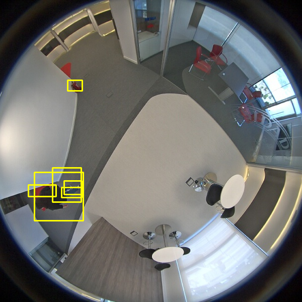
(b) $\sigma=0.3$

(c) $\sigma=0.5$

(d) $\sigma=0.7$

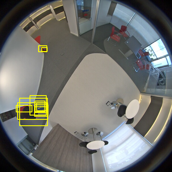
(e) $\sigma=0.9$

$C_{t}=0.8$

0.195].19

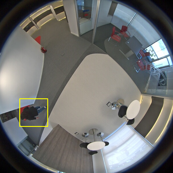
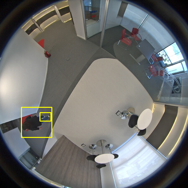
Figure 1: Visualization of results for Soft-NMS with the Gaussian penalty function on an omnidirectional image from the PIROPO database. The columns are varied over different $\sigma$ of the Gaussian penalty function. In each row we change the confidence threshold $C_{t}$ of the Soft-NMS. See text for details.

An effect, which is easily visible is the changing number of bounding boxes in the images. In the top right corner of the matrix ($\sigma=0.9$ and $C_{t}=0.3$) the number of boxes for possible candidates of true positives is high. The opposite effect, less number of true positives with a high accuracy is observable in the bottom left corner of Figure 1 (values of $\sigma=0.1$ or $\sigma=0.3$ and $C_{t}=0.8$). Using $\sigma$ for the steering of the smoothness of the merging of the bounding boxes makes the effects explainable. The higher we select $\sigma$, the closer comes the exponential function in (12) to 1. Is the exponential function close to or equal to 1, the number of boxes does not change. With the knowledge, that the exponential function cannot become zero, the smaller we set $\sigma$, the smaller is the number of the bounding boxes in the final set $\mathcal{D}$. The Gaussian smoothing function in the Soft-NMS delivers the best results, compared to the other variants of NMS.

6.2 Ground Truth Evaluation

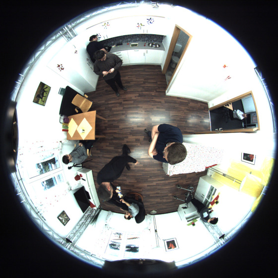
(a) input data

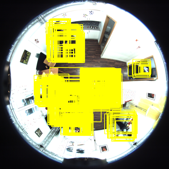
(b) raw detection boxes

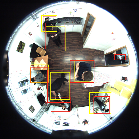
(c) ground truth (red), detection (yellow)

Figure 2: Detection result on omnidirectional images for the class person on the Flat dataset.

A well working example of our approach is shown in Figure 2. In Figure 2(a) we show an omnidirectional input image from our own dataset. The raw detections of YOLOv2 with a high number of possible true positive candidates without NMS is visualized in Figure 2(b). The final detection result after the bounding box refinement is shown in Figure 2(c). We apply Soft-NMS with a Gaussian smoothing function. The ground truth evaluation is done through manually annotated bounding box as shown in Figure 2(c).

As scalar evaluation metrics for the detector’s result we choose precision and recall [Szeliski, 2010], which leads to precision-recall (PR) curves. Additionally, we determine the AP [Szeliski, 2010]. Based on our application we concentrate on the class person, that makes the use of mAP obsolete for evaluation.

The precision and recall are based on the three basic error rates, namely the true positives (TP), the false positives (FP) and the false negatives (FN). Based on the number of these values per frame in the dataset the precision $\mathit{pr}$ and recall $\mathit{re}$ are given by:

$$\mathit{pr}=\frac{\#TP}{\#TP+\#FP}\text{\quad and \quad}\mathit{re}=\frac{\#TP}{\#TP+\#FN}.$$ (13)

Ideally, the $\mathit{pr}$ and $\mathit{re}$ values in (13) are close to one, each. The higher the values of the evaluation metrics, the larger the area under the PR curve, the better the performance of the detector.

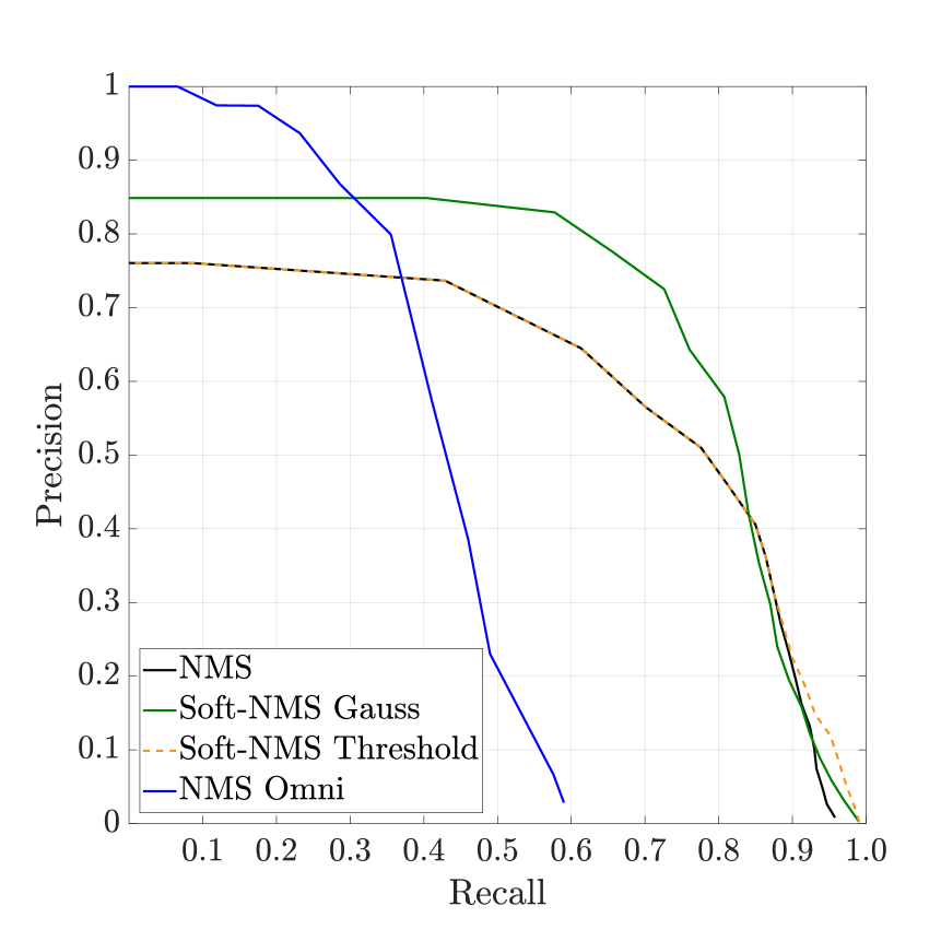
(a) Precision-recall curve on PIROPO

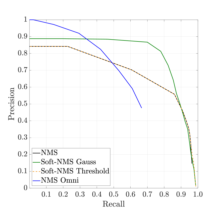
(b) Precision-recall curve on our own data (Flat)

Figure 3: The precision-recall curve for NMS, Soft-NMS and Soft-NMS with Gaussian smoothing function on two different omnidirectional image datasets from back-projected perspective views. The precision-recall curve of NMS Omni show the direct application of YOLOv2 to the omnidirectional images. $O_{t}=0.5$ is the overlap threshold for the IoU from the resulting detection box to the ground truth box.

The PR curves in Figure 3 show the evaluation of our method with manually generated ground truth. The parameter $O_{t}$ is the overlap threshold for the IoU from the resulting detection box to the ground truth box. We consider the PR curves for NMS, Soft-NMS and Soft-NMS with a Gaussian smoothing function on omnidirectional images from back-projected perspective views and compare them to the results of the direct application of YOLOv2 to the omnidirectional images, namely NMS Omni.

The steepest curve in Figure 3 is NMS Omni that reaches a precision of 1 at small recall. The constellation validates our observations, that the YOLOv2 detector localizes the objects in omnidirectional images accurate with a high number of false negatives.

Table 1: Evaluation on PIROPO and Flat dataset with average precision for class person

	PIROPO	Flat
NMS	56.6	68.3
Soft-NMS Gauss	64.6	77.6
Soft-NMS	57.1	68.1
Omni	41.4	69.6

For further quantitative evaluation we compute the AP that is the area under the PR curves of Figure 3 and visualized in Table 1. The overlap threshold $O_{t}=0.5$ follows the PASCAL VOC notation [Everingham et al., 2010]. Additionally, we determine the weighted mean values of precision for NMS, Soft-NMS with Gaussian smoothing, Soft-NMS and apply YOLOv2 to the omnidirectional images directly. The best (i.e. highest) value of AP is highlighted in bold. We reach an AP for the class person of $64.6\%$ through Soft-NMS with a Gaussian smoothing function on PIROPO and $77.6\%$ on the $Flat$ Dataset, respectively.

Salient points of the PR curves in Figure 3 are intersections of the worst performing and the highest performing approach. Looking at the NMS Omni graph (blue) and the Soft-NMS Gauss graph (blue) we observe an intersection at a precision of $0.83$ and recall of $0.35$. From this point up to recall of $0.75$ the bounding box refinement method with Soft-NMS Gauss outperforms all other curves without significant decrease of precision on PIROPO.

Another people detector on omnidirectional images is [Krams and Kiryati, 2017] that use DET curves on BOMNI database [Demiröz et al., 2012] for evaluation, therefore we don’t compare our results to this people detection approach. Due to unavailable public training datasets with labeled fish-eye images, we did not do fine-tuning of YOLOv2 from initial weights with omnidirectional image data.

We make the following observations. After the back projection from the perspective to the omnidirectional view bounding boxes are oversized, because the axis parallelism is not preserved. Through forcing parallel box edges with respect to the axis in the omnidirectional image coordinate system, we do not receive minimal enclosing rectangles.

For the most of the recall and precision values the graphs of NMS and Soft-NMS are equal. Only at precisions smaller than $0.2$ we observe different trends as shown in Figure 3.

7 Conclusion

In this work we present a method to detect persons in omnidirectional images based on CNNs. We apply a state-of-the-art object detector, namely YOLOv2, to virtual perspective views and transform the detections back to the omnidirectional source images. For the transformation the step size of the two angles, azimuth and elevation was selected in a way, that the perspective images are highly overlapped. In contrast to the standard implementation of YOLOv2 we use the raw detection boxes instead of applying a NMS as bounding box refinement at the end of the network. After back projection from perspective to omnidirectional images we apply three different NMS methods for pruning the back-projected bounding boxes based on confidence and overlap.

We evaluated the bounding box refinement methods, NMS, Soft-NMS with a threshold and Soft-NMS with Gaussian smoothing on our manually generated ground truth on the PIROPO database and the Flat dataset using PR curves and AP. At $O_{t}=0.5$ we reach an AP for the class person of $64.6\%$ on PIROPO and $77.6\%$ on Flat through Soft-NMS with Gaussian smoothing.

Based on the work of transformation from omnidirectional to perspective and vice versa there are a couple of ideas for future work. One of our central questions is: how the detection rate of the object detector changes if we consider the lens distortion parameters?

To close the gap of missing omnidirectional ground truth, we will create labeled synthetic and real-world data. To simplify the data generation we can use our approach followed by manual refinement of detections to create ground truth on omnidirectional images. To improve the approach at the point of projecting bounding boxes from perspective to omnidirectional model it is necessary to minimize the effect of oversized boxes in omnidirectional images.

References

- Bodla et al., 2017 Bodla, N., Singh, B., Chellappa, R., and Davis, L. S. (2017). Soft-nms - improving object detection with one line of code. In IEEE International Conference on Computer Vision, ICCV 2017, Venice, Italy, October 22-29, 2017, pages 5562–5570.
- Cinaroglu and Bastanlar, 2014 Cinaroglu, I. and Bastanlar, Y. (2014). A direct approach for human detection with catadioptric omnidirectional cameras. In Signal Processing and Communications Applications Conference (SIU), 2014 22nd, pages 2275–2279. IEEE.
- Cohen et al., 2018 Cohen, T. S., Geiger, M., Köhler, J., and Welling, M. (2018). Spherical CNNs. In International Conference on Learning Representations.
- Dai et al., 2016 Dai, J., Li, Y., He, K., and Sun, J. (2016). R-FCN: object detection via region-based fully convolutional networks. In Advances in Neural Information Processing Systems 29: Annual Conference on Neural Information Processing Systems 2016, December 5-10, 2016, Barcelona, Spain, pages 379–387.
- del Blanco and Carballeira, 2016 del Blanco, C. R. and Carballeira, P. (2016). The piropo database (people in indoor rooms with perspective and omnidirectional cameras). https://sites.google.com/site/piropodatabase/, unpublished dataset.
- Demiröz et al., 2012 Demiröz, B. E., İsmail Ari, Eroğlu, O., Salah, A. A., and Akarun, L. (2012). Feature-based tracking on a multi-omnidirectional camera dataset. In 2012 5th International Symposium on Communications, Control and Signal Processing, pages 1–5.
- Everingham et al., 2010 Everingham, M., Gool, L. J. V., Williams, C. K. I., Winn, J. M., and Zisserman, A. (2010). The pascal visual object classes (VOC) challenge. International Journal of Computer Vision, 88(2):303–338.
- Findeisen et al., 2013 Findeisen, M., Meinel, L., Heß, M., Apitzsch, A., and Hirtz, G. (2013). A fast approach for omnidirectional surveillance with multiple virtual perspective views. In Proceedings of Eurocon 2013, International Conference on Computer as a Tool, Zagreb, Croatia, July 1-4, 2013, pages 1578–1585.
- Girshick et al., 2013 Girshick, R. B., Donahue, J., Darrell, T., and Malik, J. (2013). Rich feature hierarchies for accurate object detection and semantic segmentation. CoRR, abs/1311.2524.
- Hartley and Zisserman, 2006 Hartley, R. and Zisserman, A. (2006). Multiple view geometry in computer vision (2. ed.). Cambridge University Press.
- He et al., 2016 He, K., Zhang, X., Ren, S., and Sun, J. (2016). Deep residual learning for image recognition. In 2016 IEEE Conference on Computer Vision and Pattern Recognition, CVPR 2016, Las Vegas, NV, USA, June 27-30, 2016, pages 770–778.
- Krams and Kiryati, 2017 Krams, O. and Kiryati, N. (2017). People detection in top-view fisheye imaging. In 2017 14th IEEE International Conference on Advanced Video and Signal Based Surveillance (AVSS), pages 1–6.
- Krasin et al., 2017 Krasin, I., Duerig, T., Alldrin, N., Ferrari, V., Abu-El-Haija, S., Kuznetsova, A., Rom, H., Uijlings, J., Popov, S., Veit, A., Belongie, S., Gomes, V., Gupta, A., Sun, C., Chechik, G., Cai, D., Feng, Z., Narayanan, D., and Murphy, K. (2017). Openimages: A public dataset for large-scale multi-label and multi-class image classification. Dataset available from https://github.com/openimages.
- Lee et al., 2018 Lee, S., Sung, J., Yu, Y., and Kim, G. (2018). A memory network approach for story-based temporal summarization of videos. In Proceedings of the IEEE Conference on Computer Vision and Pattern Recognition, pages 1410–1419.
- Li et al., 2017 Li, W., Wang, L., Li, W., Agustsson, E., and Gool, L. V. (2017). Webvision database: Visual learning and understanding from web data. CoRR, abs/1708.02862.
- Lin et al., 2014 Lin, T., Maire, M., Belongie, S. J., Hays, J., Perona, P., Ramanan, D., Dollár, P., and Zitnick, C. L. (2014). Microsoft COCO: common objects in context. In Computer Vision - ECCV 2014 - 13th European Conference, Zurich, Switzerland, September 6-12, 2014, Proceedings, Part V, pages 740–755.
- Liu et al., 2016 Liu, W., Anguelov, D., Erhan, D., Szegedy, C., Reed, S. E., Fu, C., and Berg, A. C. (2016). SSD: Single Shot MultiBox Detector, pages 21–37.
- Redmon et al., 2016 Redmon, J., Divvala, S. K., Girshick, R. B., and Farhadi, A. (2016). You only look once: Unified, real-time object detection. In 2016 IEEE Conference on Computer Vision and Pattern Recognition, CVPR 2016, Las Vegas, NV, USA, June 27-30, 2016, pages 779–788.
- Redmon and Farhadi, 2017 Redmon, J. and Farhadi, A. (2017). YOLO9000: better, faster, stronger. In 2017 IEEE Conference on Computer Vision and Pattern Recognition, CVPR 2017, Honolulu, HI, USA, July 21-26, 2017, pages 6517–6525.
- Ren et al., 2015 Ren, S., He, K., Girshick, R. B., and Sun, J. (2015). Faster R-CNN: towards real-time object detection with region proposal networks. In Cortes, C., Lawrence, N. D., Lee, D. D., Sugiyama, M., and Garnett, R., editors, Advances in Neural Information Processing Systems 28: Annual Conference on Neural Information Processing Systems 2015, December 7-12, 2015, Montreal, Quebec, Canada, pages 91–99.
- Russakovsky et al., 2015 Russakovsky, O., Deng, J., Su, H., Krause, J., Satheesh, S., Ma, S., Huang, Z., Karpathy, A., Khosla, A., Bernstein, M. S., Berg, A. C., and Li, F. (2015). Imagenet large scale visual recognition challenge. International Journal of Computer Vision, 115(3):211–252.
- Szeliski, 2010 Szeliski, R. (2010). Computer Vision: Algorithms and Applications. Springer-Verlag New York, Inc., New York, NY, USA, 1st edition.