Learning What Information to Give in
Partially Observed Domains

Abstract

In many robotic applications, an autonomous agent must act within and explore a partially observed environment that is unobserved by its human teammate. We consider such a setting in which the agent can, while acting, transmit declarative information to the human that helps them understand aspects of this unseen environment. In this work, we address the algorithmic question of how the agent should plan out what actions to take and what information to transmit. Naturally, one would expect the human to have preferences, which we model information-theoretically by scoring transmitted information based on the change it induces in weighted entropy of the human’s belief state. We formulate this setting as a belief mdp and give a tractable algorithm for solving it approximately. Then, we give an algorithm that allows the agent to learn the human’s preferences online, through exploration. We validate our approach experimentally in simulated discrete and continuous partially observed search-and-recover domains. Visit http://tinyurl.com/chitnis-corl-18 for a supplementary video.

Keywords: belief space planning, information theory, human-robot interaction

1 Introduction

Consider a scenario where a human operator must manage several autonomous search-and-rescue agents that can move through, observe, and modify their respective environments, which are sites of recent disasters. The agents have highly important objectives: to rescue trapped victims. Secondarily, they should keep the human operator informed about what is taking place, but should not sacrifice their primary objective just to transmit information. Rather than receiving a continuous stream of data such as a video feed from each agent, from which it would be hard to extract salient findings, the human may only want to receive important information, forcing the agents to make decisions about what information is worth giving. Naturally, the human will have preferences about what information is important to them: for instance, they would want to be notified when an agent encounters a victim, but probably not every time it encounters a pile of rubble.

In this work, we address the algorithmic question of how an agent should plan out what actions to take in the world and what information to transmit. We treat this problem as a sequential decision task where on each timestep the agent can choose to transmit information, while also acting in the world. To capture the notion that the human has preferences, we model the human as an entity that scores the agent based on how interesting the transmitted information is to them. The agent’s primary objective is to act optimally in the world; secondarily, it should transmit score-maximizing information while acting. We formulate this setting as a decomposable belief Markov decision process (belief mdp) and give a tractable algorithm for solving it approximately in practice.

We model the human’s score function information-theoretically. First, we suppose that the human maintains a belief state, a probability distribution over the set of possible environment states; this belief gets updated based on information received from the agent. Next, we let the human’s score for a given piece of information be a function of the change in weighted entropy induced by the belief update. This weighting is a crucial aspect of our approach: it allows the human to describe, in a natural way, which aspects of the environment they want to be informed about.

We give an algorithm that allows the agent to learn the human’s preferences online, through exploration. In this setting, online learning is very important: the agent must explore in order to discover the human’s preferences, by giving them a variety of information. We validate our approach experimentally in simulated discrete and continuous partially observed search-and-recover domains, and find that our belief mdp framework and corresponding planning and learning algorithms are effective in practice. Visit http://tinyurl.com/chitnis-corl-18 for a supplementary video.

2 Related Work

The problem setting we consider, in which an agent must act optimally in its environment while secondarily giving information that optimizes a human’s score function, is novel but has connections to several related problems in human-robot interaction. Our work is unique in using weighted entropy to capture the human’s preferences over which aspects of the environment are important.

Information-theoretic perspective on belief updates. The idea of taking actions that lower the entropy of a belief state has been studied in robotics for decades. Originally, it was applied to navigation [1] and localization [2]. More recently, it has also been used in human-robot interaction settings [3, 4]: the robot asks the human clarifying questions about its environment to lower the entropy of its own belief, which helps it plan more safely and robustly. By contrast, in our method the robot is concerned with estimating the entropy of the human’s belief, like in work by Roy et al. [5].

Estimating the human’s mental state. Having a robot make decisions based on its current estimate of the human’s mental state has been studied in human-robot collaborative settings [6, 7, 8]. The robot first estimates the human’s belief about the world state and goal, then uses this information to build a human-aware policy for the collaborative task. This strategy allows the robot to exhibit desirable behavior, such as signaling its intentions in order to avoid surprising the human.

Modeling user preferences with active learning. The idea of using active learning to understand user preferences has received significant attention [9, 10, 11]. Typically in these methods, the agent gathers information from the user through some channel, estimates a reward function from this information, and acts based on this estimated reward. Our method for learning the human’s preferences online works similarly, but we assume that the reward has an information-theoretic structure.

3 Background

3.1 Partially Observable Markov Decision Processes and Belief States

Our work considers agent-environment interaction in the presence of uncertainty, which is often formalized as a partially observable Markov decision process (pomdp) [12]. An undiscounted pomdp is a tuple $\langle\mathcal{S},\mathcal{A},\Omega,T,O,R\rangle$: $\mathcal{S}$ is the state space; $\mathcal{A}$ is the action space; $\Omega$ is the observation space; $T(s,a,s^{\prime})=P(s^{\prime}\mid s,a)$ is the transition distribution with $s,s^{\prime}\in\mathcal{S},a\in\mathcal{A}$; $O(s,o)=P(o\mid s)$ is the observation model with $s\in\mathcal{S},o\in\Omega$; and $R(s,a,s^{\prime})$ is the reward function with $s,s^{\prime}\in\mathcal{S},a\in\mathcal{A}$. Some states in $\mathcal{S}$ are said to be terminal, ending the episode and generating no further reward. The agent’s objective is to maximize its overall expected reward, $\mathbb{E}\left[\sum_{t}R(s_{t},a_{t},s_{t+1})\right]$. The optimal solution to a pomdp is a policy that maps the history of observations and actions to the next action to take, such that this objective is optimized. Exact solutions for interesting pomdps are typically infeasible to compute, but some popular approximate approaches are online planning [13, 14, 15] and finding a policy offline with a point-based solver [16, 17].

The sequence of states $s_{0},s_{1},...$ is unobserved, so the agent must instead maintain a belief state, a probability distribution over the space of possible states. This belief is updated on each timestep, based on the received observation and taken action. Unfortunately, representing this distribution exactly is prohibitively expensive for even moderately-sized pomdps. One typical alternative representation is a factored one, in which we assume the state can be decomposed into variables (features), each with a value; the factored belief then maps each variable to a distribution over possible values.

A Markov decision process (mdp) $\langle\mathcal{S},\mathcal{A},T,R\rangle$ is a simplification of a pomdp where the states are fully observed by the agent, so $\Omega$ and $O$ are not needed. The optimal solution to an mdp is a policy that maps the state to the next action to take, such that the same objective as before is optimized.

Every pomdp $\langle\mathcal{S},\mathcal{A},\Omega,T,O,R\rangle$ induces an mdp $\langle\mathcal{B},\mathcal{A},\tau,\rho\rangle$ on the belief space, known as a belief mdp, where: $\mathcal{B}$ is the space of beliefs $B$ over $\mathcal{S}$; $\tau(B,a,B^{\prime})=\sum_{o\in\Omega}P(B^{\prime}\mid B,a,o)P(o\mid B,a)$; and $\rho(B,a,B^{\prime})=\mathbb{E}_{s\sim B,s^{\prime}\sim B^{\prime}}R(s,a,s^{\prime})$. See Kaelbling et al. [12] for details.

3.2 Weighted Entropy and Weighted Information Gain

Weighted entropy is a generalization of Shannon entropy that was first presented and analyzed by Guiaşu [18]. The Shannon entropy of a discrete probability distribution $p$, given by $S(p)=\mathbb{E}\left[-\log p_{i}\right]=-\sum_{i:p_{i}\neq 0}p_{i}\log p_{i}$, is a measure of the expected amount of information carried by samples from the distribution, and can also be viewed as a measure of the distribution’s uncertainty. Note that trying to replace the summation with integration for continuous distributions would not be valid, because the interpretation of entropy as a measure of uncertainty gets lost; e.g., the integral can be negative. The information gain in going from a distribution $p$ to another $p^{\prime}$ is $S(p)-S(p^{\prime})$.

Definition 1.

The weighted entropy of a discrete probability distribution $p$ is given by $S_{w}(p)=-\sum_{i:p_{i}\neq 0}w_{i}p_{i}\log p_{i}$, where all $w_{i}\geq 0$. The weighted information gain in going from a distribution $p$ to another $p^{\prime}$ is $S_{w}(p)-S_{w}(p^{\prime})$.

Weighted entropy allows certain values of the distribution to heuristically have more impact on the uncertainty, but cannot be interpreted as the expected amount of information carried by samples.

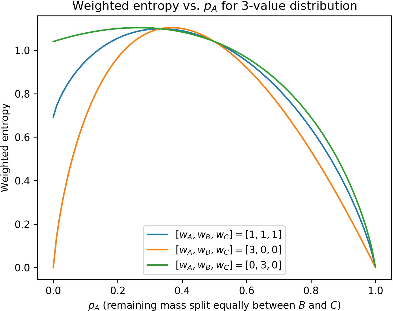
Figure 1: Weighted entropy for a distribution with three values: $A,B,C$. The x-axis varies $p_{A}$, with the remaining probability mass split equally between $B$ and $C$.

Intuition. Figure 1 helps give intuition about weighted entropy by plotting it for the case of a distribution with three values. In the figure, we only let $p_{A}$ vary freely and set $p_{B}=p_{C}=\frac{1-p_{A}}{2}$, so that the plot can be visualized in two dimensions. When only one value is possible ($p_{A}=1$), the entropy is always 0 regardless of the setting of weights, but as $p_{A}$ approaches 1 from the left, the entropy drops off more quickly the higher $w_{A}$ is (relative to $w_{B}$ and $w_{C}$). If all weight is placed on $A$ (the orange curve), then when $p_{A}=0$ the entropy also goes to 0, because the setting of weights conveys that distinguishing between $B$ and $C$ gives no information. However, if no weight is placed on $A$ (the green curve), then when $p_{A}=0$ we have $p_{B}=p_{C}=0.5$, and the entropy is high because the setting of weights conveys that all of the information lies in telling $B$ and $C$ apart.

4 Problem Setting

We formulate our problem setting as a belief mdp (Section 3.1) from the agent’s perspective, then give an algorithm for solving it approximately. At each timestep, the agent takes an action in the environment and chooses a piece of information $i$ (or null if it chooses not to give any) to transmit, along with the marginal probability, $B_{A}(i)$, of $i$ under the agent’s current belief. See Figure 2.

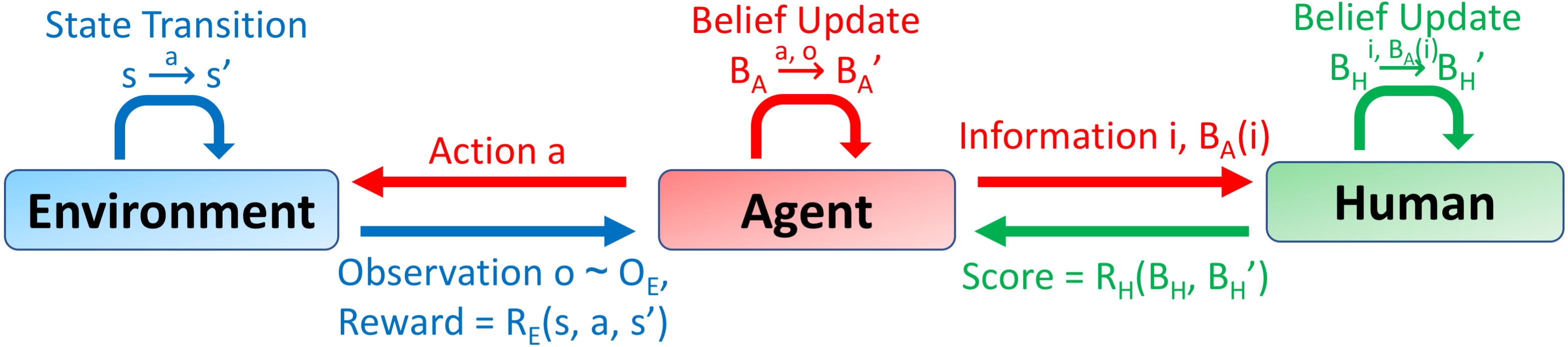
Figure 2: A diagram of our problem setting. Red: agent’s activities; blue: environment’s; green: human’s.

Our presentation of the formulation will assume that the agent knows 1) the human’s initial belief, 2) the model for how the human updates their belief, and 3) that only information from the agent can induce belief updates; this assumption effectively renders the human’s belief state fully observed by the agent. We can easily relax this assumption: suppose the agent were allowed to query only some aspects of the human’s belief; then, it could incorporate the remainder into its own belief as part of the latent state. We will not complicate our presentation by describing this setting explicitly.

4.1 Belief mdp Formulation

Let the agent-environment interaction be modeled as a pomdp $\langle\mathcal{S}_{E},\mathcal{A}_{E},\Omega_{E},T_{E},O_{E},R_{E}\rangle$, where $\mathcal{S}_{E}$ is continuous or discrete. This induces a belief mdp $\langle\mathcal{B}_{E},\mathcal{A}_{E},\tau_{E},\rho_{E}\rangle$, where $\mathcal{B}_{E}$ is the space of beliefs over $\mathcal{S}_{E}$. The agent maintains a belief state $B_{A}\in\mathcal{B}_{E}$, updated with a Bayes filter [19].

The human maintains their own belief state $B_{H}\in\mathcal{B}_{E}$ over environment states, updated based only on information transmitted by the agent, and gives the agent a real-valued score on each timestep for this information. We model the human as a tuple $\langle\mathcal{I},T_{H},B_{H}^{0},R_{H}\rangle$: $\mathcal{I}$ is a set of fluents (Boolean atoms that may or may not hold in the state) that defines the space of information the agent can transmit; $T_{H}(s,s^{\prime})=P(s^{\prime}\mid s)$ is the human’s forward model of the world with $s,s^{\prime}\in\mathcal{S}_{E}$; $B_{H}^{0}\in\mathcal{B}_{E}$ is the human’s initial belief; and $R_{H}(B_{H},B_{H}^{\prime})$ is the human’s score function with $B_{H},B_{H}^{\prime}\in\mathcal{B}_{E}$. The $T_{H}$ allows the human to model the degradation of information over time; we use a simple $T_{H}$ that is almost the identity function, but gives $\epsilon$ probability to non-identity transitions.

At each timestep, the agent selects information $i\in\mathcal{I}$ to give and transmits it along with the marginal probability of $i$ under $B_{A}$, defined as $B_{A}(i)=\sum_{s\in\mathcal{S}_{E}:i\text{ holds in }s}B_{A}(s)$. We update the belief $B_{H}$ according to Jeffrey’s rule [20], which is based on the principle of probability kinematics for minimizing the change in belief. First, we define $\tilde{B}_{H}(s)=\sum_{s^{\prime}\in\mathcal{S}_{E}}T_{H}(s^{\prime},s)B_{H}(s^{\prime}),\forall s\in\mathcal{S}_{E}$. Then the full belief update, $B_{H}\to B_{H}^{\prime}$, is $B_{H}^{\prime}(s)=\frac{\tilde{B}_{H}(s)B_{A}(i)}{\tilde{B}_{H}(i)}$ if $i$ holds in $s$ and $\frac{\tilde{B}_{H}(s)(1-B_{A}(i))}{1-\tilde{B}_{H}(i)}$ if $i$ does not hold in $s$, $\forall s\in\mathcal{S}_{E}$. The summations can be replaced with integration if $\mathcal{S}_{E}$ is continuous.

Objective. We define the agent’s objective as follows: to act optimally in the environment (maximizing the expected sum of rewards $R_{E}$) and, subject to acting optimally, to give information such that the expected sum of the human’s scores $R_{H}$ over the trajectory is maximized.

The full belief mdp $\mathcal{P}$ for this setting (from the agent’s perspective) is a tuple $\langle\mathcal{B},\mathcal{A},\tau,\rho\rangle$:

• $\mathcal{B}=\mathcal{B}_{E}\times\mathcal{B}_{E}$. A state is a pair of the agent’s belief $B_{A}\in\mathcal{B}_{E}$ and the human’s belief $B_{H}\in\mathcal{B}_{E}$.

• $\mathcal{A}=\mathcal{A}_{E}\times\mathcal{I}$. An action is a pair of environment action $a\in\mathcal{A}_{E}$ and information $i\in\mathcal{I}$.

• $\tau(\langle B_{A},B_{H}\rangle,\langle a,i\rangle,\langle B_{A}^{\prime},B_{H}^{\prime}\rangle)=\tau_{E}(B_{A},a,B_{A}^{\prime})$ if $B_{H}^{\prime}$ satisfies the update equation, else 0.

• $\rho(\langle B_{A},B_{H}\rangle,\langle a,i\rangle,\langle B_{A}^{\prime},B_{H}^{\prime}\rangle)$ is a pair $\langle\rho_{E}(B_{A},a,B_{A}^{\prime}),R_{H}(B_{H},B_{H}^{\prime})\rangle$ with the comparison operation $\langle x_{1},y_{1}\rangle>\langle x_{2},y_{2}\rangle\iff x_{1}>x_{2}\lor(x_{1}=x_{2}\land y_{1}>y_{2})$; similarly for $<$.

The following algorithm for solving $\mathcal{P}$ by decomposition will help us give an approximation next.

Algorithm DecomposeAndSolve($\mathcal{P}$)

      1 $\pi_{\text{act}}\leftarrow$ (solve agent-environment belief mdp $\langle\mathcal{B}_{E},\mathcal{A}_{E},\tau_{E},\rho_{E}\rangle$)

      2 // Define $\tau_{H}$ as $\tau_{H}(\langle B_{A},B_{H}\rangle,i,\langle B_{A}^{\prime},B_{H}^{\prime}\rangle)=\tau(\langle B_{A},B_{H}\rangle,\langle\pi_{\text{act}}(B_{A}),i\rangle,\langle B_{A}^{\prime},B_{H}^{\prime}\rangle)$.

      3 // Define $\rho_{H}$ as $\rho_{H}(\langle B_{A},B_{H}\rangle,i,\langle B_{A}^{\prime},B_{H}^{\prime}\rangle)=R_{H}(B_{H},B_{H}^{\prime})$.

      4 $\pi_{\text{info}}\leftarrow$ (solve agent-human belief mdp $\langle\mathcal{B}_{E}\times\mathcal{B}_{E},\mathcal{I},\tau_{H},\rho_{H}\rangle$)

      5 return policy $\pi$ for $\mathcal{P}$: $\pi(\langle B_{A},B_{H}\rangle)=\langle\pi_{\text{act}}(B_{A}),\pi_{\text{info}}(\langle B_{A},B_{H}\rangle)\rangle$

      

Algorithm 1 Algorithm for solving $\mathcal{P}$ by decomposition. The agent-human belief mdp must include the agent’s belief $B_{A}$ in the state so that the marginal probabilities of information, $B_{A}(i)$, can be determined.

Theorem 1.

Algorithm 1 returns an optimal solution $\pi^{*}$ for $\mathcal{P}$.

Proof. Note that a policy $\pi$ for $\mathcal{P}$ maps pairs $\langle B_{A},B_{H}\rangle$ to pairs $\langle a,i\rangle$, with $a\in\mathcal{A}_{E}$ and $i\in\mathcal{I}$. We have $\pi^{*}=\operatorname*{argmax}_{\pi}\mathbb{E}\left[\sum_{t}\rho(\langle B_{A,t},B_{H,t}\rangle,\pi(\langle B_{A,t},B_{H,t}\rangle),\langle B_{A,t+1},B_{H,t+1}\rangle)\right]$. Define $\pi(\langle B_{A},B_{H}\rangle)[0]=a$, the first entry in the pair. Due to the comparison operation we defined on $\rho$, we can write $\pi^{*}=\operatorname*{argmax}_{\pi}\mathbb{E}\left[\sum_{t}\rho_{E}(B_{A,t},\pi(\langle B_{A,t},B_{H,t}\rangle)[0],B_{A,t+1})\right]$, and if there are multiple such $\pi^{*}$, pick the one that also maximizes $\mathbb{E}\left[\sum_{t}R_{H}(B_{H,t},B_{H,t+1})\right]$. The decomposition strategy exactly achieves this, by leveraging the fact that the human cannot affect the environment. ∎

4.2 Approximation Algorithm

$\mathcal{P}$ can be hard to solve optimally even using the decomposition strategy of Algorithm 1. A key challenge is that $\pi_{\text{act}}$ branches due to uncertainty about observations and transitions, so searching for the optimal $\pi_{\text{info}}$ becomes computationally infeasible. Instead, we apply the determinize-and-replan strategy [21, 22, 23], which is not optimal but often works well in practice. We determinize $\mathcal{P}$ using a maximum likelihood assumption [21], then use Algorithm 1. This procedure is repeated any time the determinization is found to have been violated. See Algorithm 2 for full pseudocode.

Line 3 generates the trajectory $\tau_{B_{A}}$ of the agent’s beliefs induced by $p_{\text{act}}$, which works because $p_{\text{act}}$ does not contain branches. Line 8 constructs a directed acyclic graph (dag) $G$ whose states are tuples of (human belief, timestep). An edge exists between $(B_{H},t)$ and $(B_{H}^{\prime},t+1)$ iff some information $i\in\mathcal{I}$ causes the belief update $B_{H}\to B_{H}^{\prime}$ under the determinized $\mathcal{P}$. The edge weight is $R_{H}(B_{H},B_{H}^{\prime})$, the human’s score for $i$. Note that all paths through $G$ have the same number of steps, and because the edge weights are the human’s scores, the longest weighted path through $G$ is precisely the information-giving plan $p_{\text{info}}$ that maximizes the total score over the trajectory. Our implementation does not build the full dag $G$; we prune the search using domain-specific heuristics.

Algorithm DecomposeAndSolveApproximate($\mathcal{P}$)

      1 $\mathcal{P}$.Determinize()

      2 $p_{\text{act}}\leftarrow$ (solve agent-environment portion of $\mathcal{P}$)

        // Acting plan (no branches).

      3 $\tau_{B_{A}}\leftarrow$ (trajectory of beliefs $B_{A}$ induced by $p_{\text{act}}$)

       Subroutine GetSuccessors(state)

            4 $(B_{H},\text{timestep})\leftarrow$ state

              // Unpack state tuple.

            5 for each $i\in\mathcal{I}$ do

                  6 $B_{H}^{\prime}\leftarrow$ (result of updating $B_{H}$ with $i$ and marginal probability $\tau_{B_{A}}[\text{timestep}](i)$)

                  7 emit next state $(B_{H}^{\prime},\text{timestep}+1)$ with edge label $i$ and weight $R_{H}(B_{H},B_{H}^{\prime})$

                  

      8$G\leftarrow$ (dag constructed from root node $(B_{H}^{0},0)$ and GetSuccessors)

      9 $p_{\text{info}}\leftarrow$ LongestWeightedPathDAG($G$)

        // Information-giving plan (no branches).

      10 return Merge($p_{\text{act}},p_{\text{info}}$)

        // Zip into a single plan.

      

Algorithm 2 Approximate approach for solving $\mathcal{P}$ with determinization. See text for detailed description.

5 Learning an Information-Theoretic Score Function

In this section, we first model the human’s score function $R_{H}$ information-theoretically using the notion of weighted entropy. Then, we give an algorithm by which the agent can learn $R_{H}$ online.

5.1 Score Function Model

We model the score function $R_{H}(B_{H},B_{H}^{\prime})$ as a function $f\in\mathbb{R}$ of the weighted information gain (Section 3.2) of the belief update induced by information:

$$R_{H}(B_{H},B_{H}^{\prime})=f(S_{w}(B_{H})-S_{w}(B_{H}^{\prime})),$$

where the $w$ are a set of weights. The human chooses both $w$ and $f$ to suit their preferences.

Assumptions. This model introduces two assumptions. 1) The human’s belief $B_{H}$, which is ideally over the environment state space $\mathcal{S}_{E}$, must be over a discrete space in order for its entropy to be well-defined. If $\mathcal{S}_{E}$ is continuous, the human can make any discrete abstraction of $\mathcal{S}_{E}$, and maintain $B_{H}$ over this abstraction instead of over $\mathcal{S}_{E}$. Note that the agent must know this discrete abstraction. 2) If the belief is factored (Section 3.1), we calculate the total entropy by summing the entropy of each factored distribution. This is an upper bound that assumes independence among the factors.

Motivation. Assuming structure in the form of $R_{H}$ makes it easier for the agent to learn the human’s preferences; the notion of weighted entropy is a compelling choice. The human’s belief state $B_{H}$ captures their perceived likelihood of each possible environment state (or value of each factor in the state). Each $p_{i}$ term in the entropy formula corresponds to an environment state or value of a factor, so the $w_{i}$ encode the human’s preferences about which states or values of factors are important.

Interpretation of $f$. Different choices of $f$ allow the human to exhibit various preferences. Choosing $f$ to be the identity function means that the human wants the agent to act greedily, transmitting the highest-scoring piece of information at each timestep. The human may instead prefer for $f$ to impose a threshold $t$: if the gain is smaller than $t$, then $f$ could return a negative score to penalize the agent for not being sufficiently informative. A sublinear $f$ rewards the agent for splitting up information into subparts and transmitting it over multiple timesteps, while a superlinear $f$ rewards the agent for withholding partial information in favor of occasionally transmitted, more complete information.

5.2 Learning Preferences Online

We now give Algorithm 3, which allows the agent to learn $w$ and $f$ online through exploration. This algorithm works for both single-episode lifelong learning problems where no states are terminal and short-horizon problems where the agent must learn over several episodes. In Line 7, the agent explores the human’s preferences using an $\epsilon$-greedy policy that gives a random piece of information with probability $\epsilon$ and otherwise follows $\pi$, the policy solving $\mathcal{P}$ under the current $\hat{w}$ and $\hat{f}$.

If the human’s preferences ($w$ or $f$) ever change, we can reset $\epsilon$ to an appropriate value and continue running the algorithm, so the agent can explore information that the human now finds interesting. Additionally, with some small modifications we can make $f$ depend on the last few timesteps of transmitted information: we need only augment states in our belief mdp with this history so it can be used to calculate $R_{H}$, and include this history in the dataset $\mathcal{D}$ used for learning in Algorithm 3.

Algorithm TrainLoop

      1 $\hat{w},\hat{f}\leftarrow$ (initial guess)

      2 $\mathcal{D}\leftarrow$ (initialize empty dataset)

      3 $\mathcal{P}\leftarrow$ (initialize problem)

        // Belief mdp described in Section 4.

      4 $\pi\leftarrow$ Solve($\mathcal{P},\hat{w},\hat{f}$)

        // Solve $\mathcal{P}$ under $\hat{w}$ and $\hat{f}$ (e.g., with Alg. 2).

      5 while not done training do

            6 Act according to $\pi$ in environment.

            7 Give information according to $\epsilon$-greedy$(\pi\;\|\;\text{random})$; obtain noisy human’s score $\tilde{s}$.

            8 Store tuple of transition and noisy score, $(B_{H},B_{H}^{\prime},\tilde{s})$, into $\mathcal{D}$.

            9 Sample training batch $T\sim\mathcal{D}$.

            10 $\mathcal{L}\leftarrow\sum_{T}(\tilde{s}-\hat{f}(S_{\hat{w}}(B_{H})-S_{\hat{w}}(B_{H}^{\prime})))^{2}/T.\text{size}$

              // Loss is mse of predicted score.

            11 Update $\hat{w},\hat{f}$ with optimization step on $\mathcal{L}$.

            12 if agent reaches terminal state then

                  13 Repeat Lines 3-4.

                  

Algorithm 3 Training loop for estimating the human’s true $w$ and $f$, given noisy supervision.

6 Experiments

We show results for three settings of the function $f$: identity, square, and natural logarithm. All three use a threshold $t=1$: if the weighted information gain is less than 1, then $f$ returns $-10$, penalizing the agent. (This threshold is arbitrary, as the weights can always be rescaled to accommodate any threshold.) If the information is null, then $f$ returns $10^{-3}$, which causes the agent to slightly prefer giving no information rather than information that induces no change in the human’s belief. We use the same weights $w$ for each factor in the belief, though this simplification is not required.

We implemented $\hat{w}$ and $\hat{f}$ in TensorFlow [24] as a single fully connected network, with hidden layer sizes [100, 50], that outputs the predicted score. The model takes as input a vector of the change, between $B_{H}$ and $B_{H}^{\prime}$, in $p_{i}\log p_{i}$ for each entry $p_{i}$ in the belief. We used a gradient descent optimizer with learning rate $10^{-1}$, $\ell_{2}$ regularization scale $10^{-7}$, sigmoid activations, batch size 100, and $\epsilon$ exponentially decaying from 1 to roughly $10^{-2}$ over the first 20 episodes.

We experiment with simulated discrete and continuous partially observed search-and-recover domains, where the agent must find and recover objects in the environment while transmitting information about these objects based on the human’s preferences. Although the pomdps we consider are simple, the aim of our experiments is to understand and analyze the nature of the transmitted information, not to require the agent to plan out long sequences of actions in the environment.

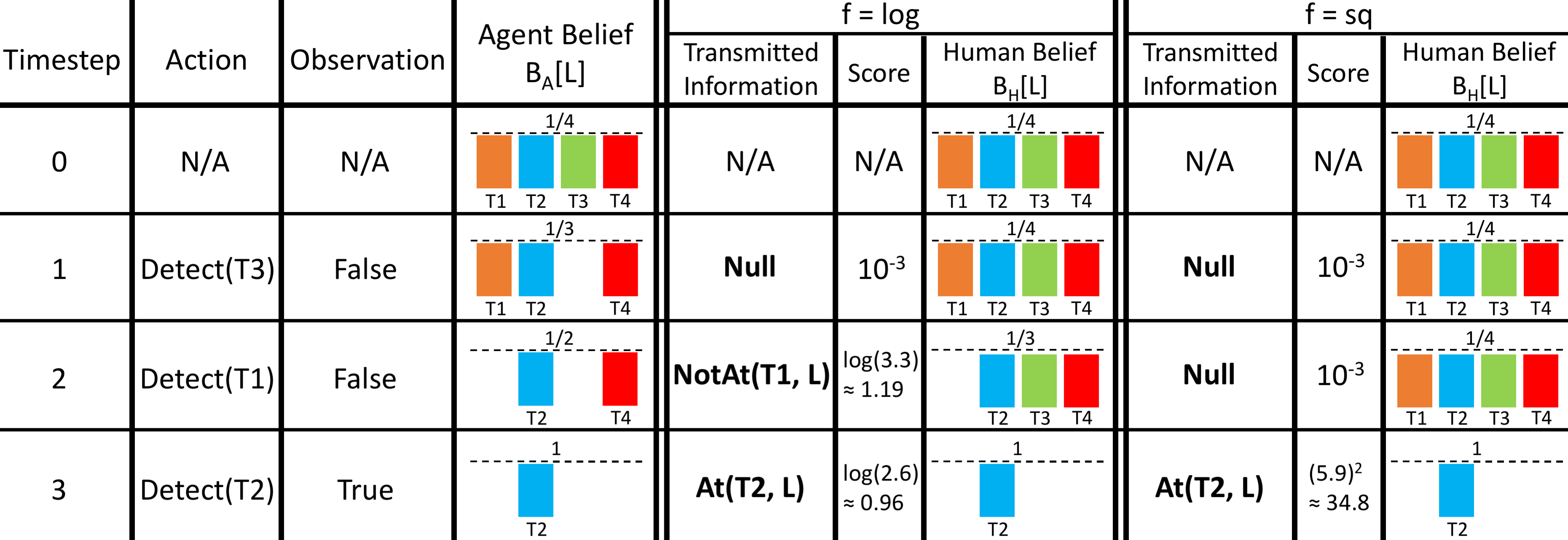
Figure 3: Example execution of Domain 1 with a single location L, showing how $w$ and $f$ affect the optimal transmitted information. For this example, the agent knows $R_{H}$ (no learning). T1, T2, T3, and T4 are the object types. At each timestep, the agent detects whether the object at L is of a particular type, and updates its belief $B_{A}$[L] accordingly. The human’s weights $w$ are {T1: 10, T2: 5, T3: 1, T4: 1}, and $f$ uses a threshold $t=1$ as discussed in the text. Agent and human beliefs are initialized uniformly over object types. Key points: (1) the agent chooses not to transmit the information NotAt(T3, L) in the second row even though it could, because T3 has low weight and thus the information gain would be too low, roughly $0.03<1$; (2) the sublinear $f$ (log) incentivizes the agent to transmit more frequently than the superlinear $f$ (sq) does, to maximize its score.

Experiment	Score from Human	# Info / Timestep	Alg. 2 Runtime (sec)
N=4, M=1, f=id	375	0.34	6.2
N=4, M=5, f=id	715	0.25	6.7
N=6, M=5, f=id	919	0.24	24.1
N=4, M=1, f=sq	13274	0.25	4.7
N=4, M=5, f=sq	33222	0.2	6.7
N=6, M=5, f=sq	41575	0.19	23.6
N=4, M=1, f=log	68	0.39	5.6
N=4, M=5, f=log	91	0.32	5.7
N=6, M=5, f=log	142	0.3	23.8

Experiment	Score from Human	# Info / Timestep	Alg. 2 Runtime (sec)
N=5, M=5, f=id	362	0.89	0.4
N=5, M=10, f=id	724	1.12	2.0
N=10, M=10, f=id	806	1.56	48.4
N=5, M=5, f=sq	37982	0.52	0.4
N=5, M=10, f=sq	99894	0.67	1.8
N=10, M=10, f=sq	109207	0.71	39.7
N=5, M=5, f=log	19	1.05	0.4
N=5, M=10, f=log	31	1.39	1.8
N=10, M=10, f=log	39	1.7	42.7

Table 1: Results on the 2D gridworld task (left) and 3D continuous task (right) for solving the mdp $\mathcal{P}$ with Algorithm 2 (no learning; $R_{H}$ is known). Each row reports averages over 100 independent trials. $N$ = grid size or number of zones, $M$ = number of objects. Planning takes time exponential in the environment size. The agent gives information less frequently when $f$ is superlinear (sq), and more when $f$ is sublinear (log).

6.1 Domain 1: Search-and-Recover 2D Gridworld Task

Our first domain is a 2D gridworld in which locations form a discrete $N\times N$ grid, $M$ objects are scattered across the environment, and the agent must find and recover all objects. Each object is of a particular type; the world of object types is known, but all types need not be present in the environment. The actions that the agent can perform on each timestep are as follows: Move by one square in a cardinal direction, with reward -1; Detect whether an object of a given type is present at the current location, with reward -5; and Recover the given object type at the current location, which succeeds with reward -20 if an object of that type is there, otherwise fails with reward -100.

An episode terminates when all $M$ objects have been recovered. To initialize an episode, we randomly assign each object a type and a unique grid location. The factored belief representation for both the agent and the human maps each grid location to a distribution over what object type (or nothing) is located there, initialized uniformly. This choice of representation implies that each $w_{i}$ in the human’s weights $w$ represents their interest in receiving information about object type $i$; for example, the human may prioritize information regarding valuable objects. The space of information $\mathcal{I}$ that the agent can select from is: At($t,l$) for every object type $t$ and location $l$; NotAt($t,l$) for every object type $t$ and location $l$; and null (no information). Our experiments vary the grid size $N$, the number of objects $M$, the human’s choice of weights $w$, and the human’s choice of $f$. Table 1, Figure 3, and Figure 4 show and discuss our results.

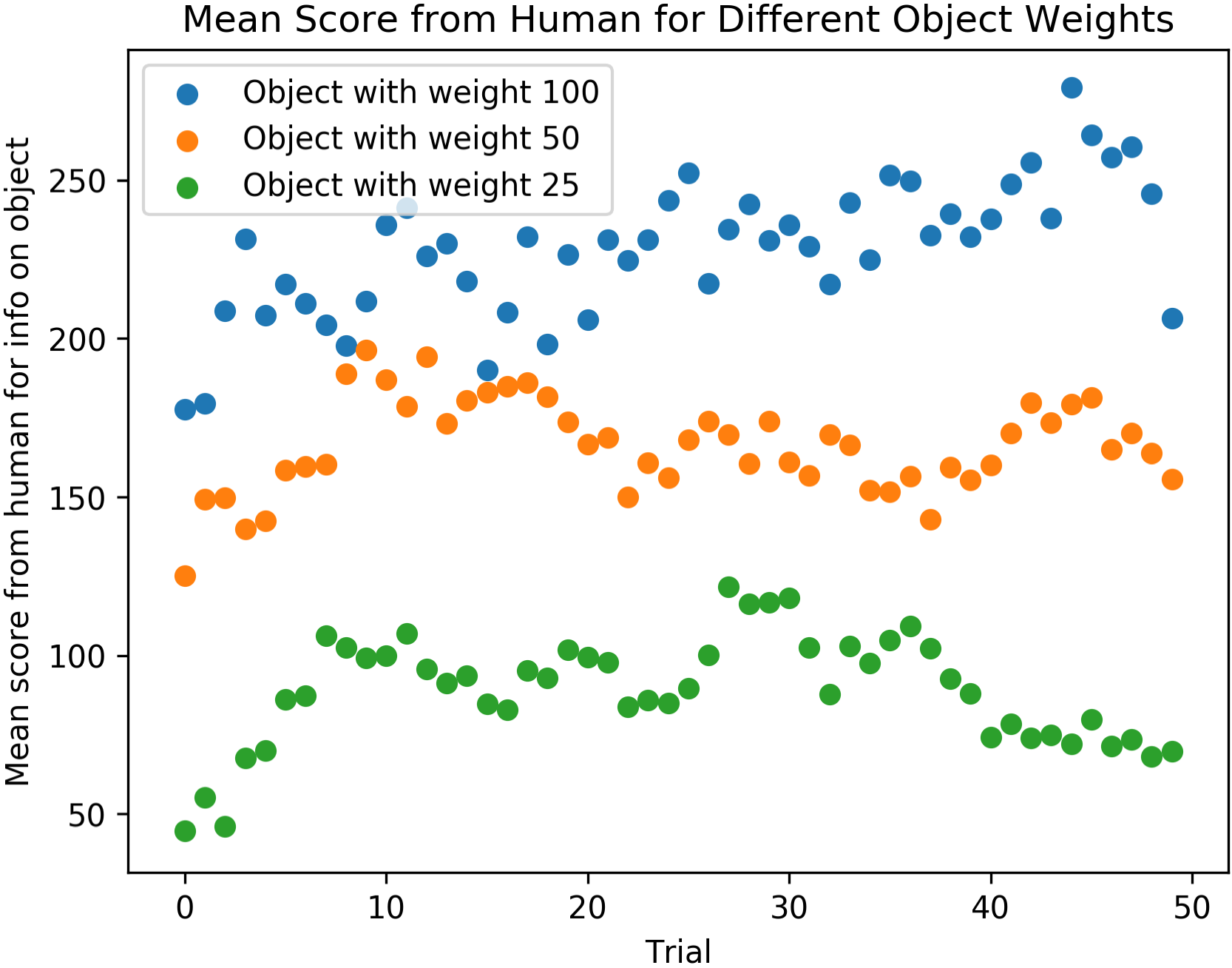
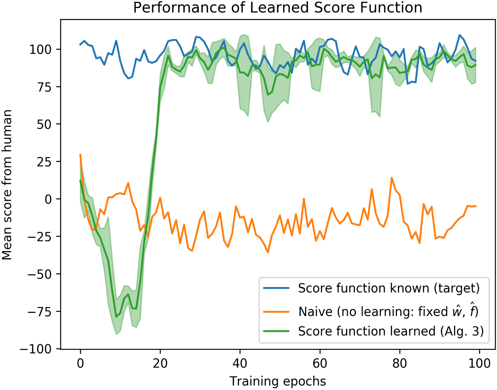
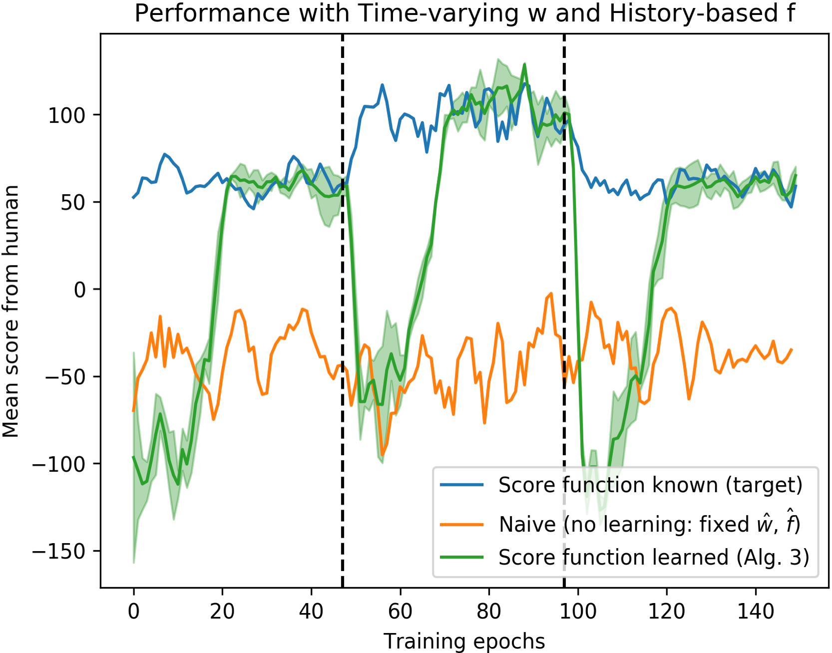
Figure 4: Domain 1 result graphs. Left. Confirming our intuition, the human gives higher scores for information about objects of higher-weighted types. These weights are chosen by the human based on their preferences. Middle. Running Algorithm 3, which learns the true score function online, allows the agent to adapt to the human’s preferences and give good information, earning itself high scores. Right. We experiment with 1) making $f$ history-based by penalizing the agent for giving information two timesteps in a row, and 2) making $w$ time-varying by changing the weights at the training epochs shown by the dotted lines. The agent learns to give good information after an exploratory period following each change in the human’s preferences. Note. Learning curves are averaged over 5 independent trials, with standard deviations shaded in green.

6.2 Domain 2: Search-and-Recover 3D Continuous Task

Our second domain is a more realistic 3D robotic environment implemented in pybullet [25]. There are $M$ objects in the world with continuous-valued positions, scattered across N “zones” which partition the position space, and the agent must find and recover all objects. The actions that the agent can perform on each timestep are as follows: Move to a given pose, with reward -1; Detect all objects within a cone of visibility in front of the current pose, with reward -5; and Recover the closest object within a cone of reachability in front of the current pose, which succeeds with reward -20 if such an object exists, otherwise fails with reward -100.

An episode terminates when all $M$ objects have been recovered. To initialize an episode, we place each object at a random collision-free position. The factored belief representation for the agent maps each known object to a distribution over its position, whereas the one for the human (which must be over a discrete space per our assumptions) maps each known object to a distribution over which of the $N$ zones it could be in; both are initialized uniformly. This choice of representation implies that each $w_{i}$ in the human’s weights $w$ represents their interest in receiving information about zone $i$; for example, the zones could represent sections of the ocean floor or rooms within a building on fire. The space of information $\mathcal{I}$ that the agent can select from is: In($o,z$) for every object $o$ and zone $z$; NotIn($o,z$) for every object $o$ and zone $z$; and null (no information). Our experiments vary the number of zones $N$, the number of objects $M$, the human’s choice of weights $w$, and the human’s choice of $f$. Table 1 and Figure 5 show and discuss our results.

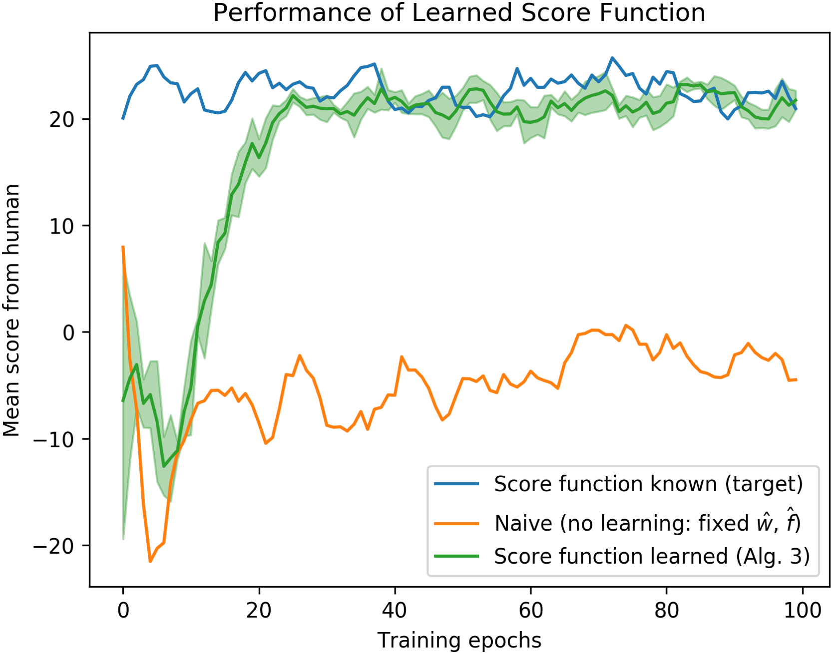
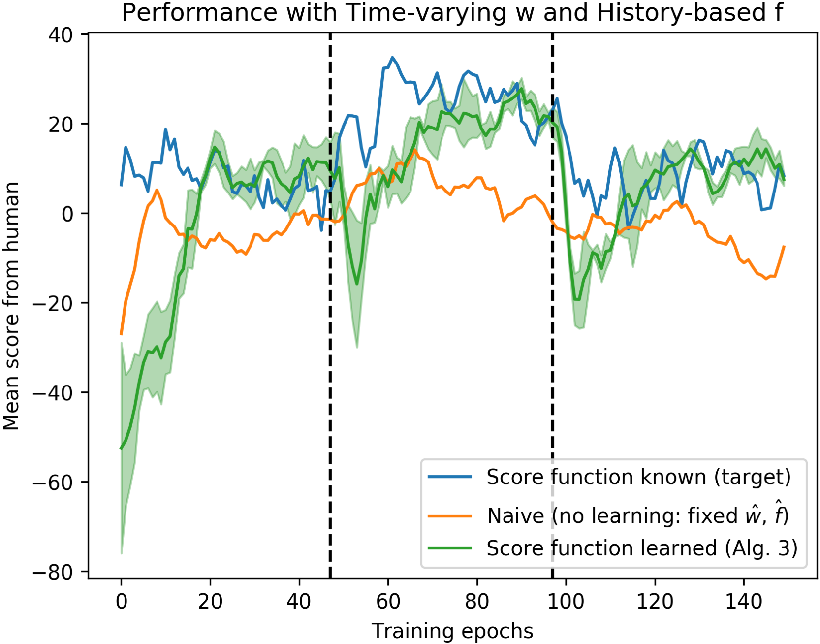
Figure 5: Domain 2 results. Left. A pybullet rendering of the task. The robot is a blue-and-orange arm, and each table is a zone. The green objects are spread across table surfaces. Middle+Right. See Figure 4 caption. Note. Learning curves are averaged over 5 independent trials, with standard deviations shaded in green.

7 Conclusion and Future Work

We have formulated a problem setting in which an agent must act optimally in a partially observed environment while learning to transmit information to a human teammate, based on their preferences. We modeled the human’s score as a function of the weighted information gain of their belief.

One direction for future work is to experiment with settings where the human has preferences over information about the different factors. Such preferences could be realized by having different scales of weights across factors, or by calculating the weighted entropy $S_{w}(B_{H})$ as a weighted sum across factors according to some other weights $v$ (rather than an unweighted sum as in this work), possibly learned. Another future direction is to have the agent learn to generate good candidates for information to transmit, rather than naively consider all available options in $\mathcal{I}$ at each timestep.

Acknowledgments

We gratefully acknowledge support from NSF grants 1420316, 1523767, and 1723381; from AFOSR grant FA9550-17-1-0165; from Honda Research; and from Draper Laboratory. Rohan is supported by an NSF Graduate Research Fellowship. Any opinions, findings, and conclusions or recommendations expressed in this material are those of the authors and do not necessarily reflect the views of our sponsors.

References

- Cassandra et al. [1996] A. R. Cassandra, L. P. Kaelbling, and J. A. Kurien. Acting under uncertainty: Discrete Bayesian models for mobile-robot navigation. In Intelligent Robots and Systems’ 96, IROS 96, Proceedings of the 1996 IEEE/RSJ International Conference on, volume 2, pages 963–972. IEEE, 1996.
- Burgard et al. [1997] W. Burgard, D. Fox, and S. Thrun. Active mobile robot localization by entropy minimization. In Advanced Mobile Robots, 1997. Proceedings., Second EUROMICRO workshop on, pages 155–162. IEEE, 1997.
- Deits et al. [2013] R. Deits, S. Tellex, P. Thaker, D. Simeonov, T. Kollar, and N. Roy. Clarifying commands with information-theoretic human-robot dialog. Journal of Human-Robot Interaction, 2(2):58–79, 2013.
- Tellex et al. [2013] S. Tellex, P. Thaker, R. Deits, D. Simeonov, T. Kollar, and N. Roy. Toward information theoretic human-robot dialog. Robotics, page 409, 2013.
- Roy et al. [2000] N. Roy, J. Pineau, and S. Thrun. Spoken dialogue management using probabilistic reasoning. In Proceedings of the 38th Annual Meeting on Association for Computational Linguistics, pages 93–100. Association for Computational Linguistics, 2000.
- Devin and Alami [2016] S. Devin and R. Alami. An implemented theory of mind to improve human-robot shared plans execution. In Human-Robot Interaction (HRI), 2016 11th ACM/IEEE International Conference on, pages 319–326. IEEE, 2016.
- Lemaignan et al. [2017] S. Lemaignan, M. Warnier, E. A. Sisbot, A. Clodic, and R. Alami. Artificial cognition for social human–robot interaction: An implementation. Artificial Intelligence, 247:45–69, 2017.
- Trafton et al. [2013] G. Trafton, L. Hiatt, A. Harrison, F. Tamborello, S. Khemlani, and A. Schultz. Act-r/e: An embodied cognitive architecture for human-robot interaction. Journal of Human-Robot Interaction, 2(1):30–55, 2013.
- Racca and Kyrki [2018] M. Racca and V. Kyrki. Active robot learning for temporal task models. In Proceedings of the 2018 ACM/IEEE International Conference on Human-Robot Interaction, pages 123–131. ACM, 2018.
- Sadigh et al. [2017] D. Sadigh, A. D. Dragan, S. Sastry, and S. A. Seshia. Active preference-based learning of reward functions. In Robotics: Science and Systems (RSS), 2017.
- Boutilier [2002] C. Boutilier. A POMDP formulation of preference elicitation problems. In AAAI/IAAI, pages 239–246, 2002.
- Kaelbling et al. [1998] L. P. Kaelbling, M. L. Littman, and A. R. Cassandra. Planning and acting in partially observable stochastic domains. Artificial intelligence, 101:99–134, 1998.
- Silver and Veness [2010] D. Silver and J. Veness. Monte-carlo planning in large POMDPs. In Advances in neural information processing systems, pages 2164–2172, 2010.
- Somani et al. [2013] A. Somani, N. Ye, D. Hsu, and W. S. Lee. DESPOT: Online POMDP planning with regularization. In Advances in neural information processing systems, pages 1772–1780, 2013.
- Bonet and Geffner [2000] B. Bonet and H. Geffner. Planning with incomplete information as heuristic search in belief space. In Proceedings of the Fifth International Conference on Artificial Intelligence Planning Systems, pages 52–61, 2000.
- Kurniawati et al. [2008] H. Kurniawati, D. Hsu, and W. S. Lee. SARSOP: Efficient point-based POMDP planning by approximating optimally reachable belief spaces. In Robotics: Science and systems, volume 2008. Zurich, Switzerland., 2008.
- Pineau et al. [2003] J. Pineau, G. Gordon, S. Thrun, et al. Point-based value iteration: An anytime algorithm for POMDPs. In IJCAI, volume 3, pages 1025–1032, 2003.
- Guiaşu [1971] S. Guiaşu. Weighted entropy. Reports on Mathematical Physics, 2(3):165–179, 1971.
- Russell and Norvig [2016] S. J. Russell and P. Norvig. Artificial intelligence: a modern approach. Malaysia; Pearson Education Limited,, 2016.
- Jeffrey [1965] R. C. Jeffrey. The logic of decision. University of Chicago Press, 1965.
- Platt Jr. et al. [2010] R. Platt Jr., R. Tedrake, L. Kaelbling, and T. Lozano-Perez. Belief space planning assuming maximum likelihood observations. 2010.
- Hadfield-Menell et al. [2015] D. Hadfield-Menell, E. Groshev, R. Chitnis, and P. Abbeel. Modular task and motion planning in belief space. In Intelligent Robots and Systems (IROS), 2015 IEEE/RSJ International Conference on, pages 4991–4998, 2015.
- Yoon et al. [2007] S. W. Yoon, A. Fern, and R. Givan. FF-Replan: A baseline for probabilistic planning. In ICAPS, volume 7, pages 352–359, 2007.
- Abadi et al. [2016] M. Abadi, P. Barham, J. Chen, Z. Chen, A. Davis, J. Dean, M. Devin, S. Ghemawat, G. Irving, M. Isard, et al. TensorFlow: A system for large-scale machine learning. In OSDI, volume 16, pages 265–283, 2016.
- Coumans et al. [2018] E. Coumans, Y. Bai, and J. Hsu. Pybullet physics engine. 2018. URL http://pybullet.org/.