Magnetostatic problems in fractal domains

Abstract.

We consider a magnetostatic problem in a 3D “cylindrical” domain of Koch type. We prove existence and uniqueness results for both the fractal and pre-fractal problems and we investigate the convergence of the pre-fractal solutions to the limit fractal one. We consider the numerical approximation of the pre-fractal problems via FEM and we give a priori error estimates. Some numerical simulations are also shown. Our long term motivation includes studying problems that appear in quantum physics in fractal domains.

Simone Creo, Maria Rosaria Lancia and Paola Vernole

Dipartimento di Scienze di Base e Applicate per l’Ingegneria, Università degli studi di Roma Sapienza,

Via A. Scarpa 16,

00161 Roma, Italy.

Michael Hinz

Department of Mathematics, Bielefeld University,

Postfach 100131,

33501 Bielefeld, Germany.

Alexander Teplyaev

Department of Mathematics, University of Connecticut,

341 Mansfield Road U1009,

06269-1009 Storrs, Connecticut, USA.

Keywords: Fractal surfaces, trace theorems, asymptotic behavior, weighted Sobolev spaces, Finite Element Method, numerical approximation.

AMS Subject Classification: Primary: 35J25, 28A80. Secondary: 35K15, 46E35, 47A07, 60J45, 65M15, 65M50, 65M60, 81Q35.

1. Introduction

The aim of this paper is to study a magnetostatic problem in a fractal domain. Trying to understand the magnetic properties of fractal structures is a new challenge from both the practical and theoretical point of view. In general mathematical physics on fractals is still a young subject, see [A, AkkermansMallick, ADT, ADT2010PRL, ADTV] for some results; magnetic operators on fractal spaces have been studied only very recently, [H14b, HR14, HTc, HKMRS17], as well as heat transfer across fractal layers or boundaries [La-Ve1, JEE, JMAA, LVSV, CPAA, nostronazarov, AR-P17, R-PGS]. Our long term motivation includes a possibility to study non-quantized penetration of magnetic field in the vortex state of superconductors [geim2000non] in fractal domains.

A mathematical theory of electrodynamics on domains with fractal boundary still has to be developed. Although many results are well known in the case of Lipschitz domains, see for instance [DautrayLions, Chapter IX], for such fractal domains even the simplest models and effects have not yet been discussed. Our considerations here should be regarded as a preliminary step in a long term project, which aims to provide theoretical and numerical studies of related physical phenomena. We believe that, beyond their theoretical interest, such results may also be useful for the construction of concrete prototypes in industrial applications, which aim to maximize (or minimize) physical quantities such as the intensity of the magnetic vector field induced by a given current density.

In the present paper we consider a linear magnetostatic problem in a cylindrical three-dimensional domain $Q=\Omega\times I$, where $\Omega$ is the two-dimensional snowflake domain with Koch-type boundary $F$ and $I$ is the unit interval. We consider the problem of finding a divergence free magnetic vector potential for given time-independent permeability and time-independent current density, and we assume that the magnetic induction vanishes outside $Q$.

Using trace and extension techniques from [jonsson91] we establish a generalized Stokes formula, see Theorem 4.4. It involves generalized tangential traces that can be expressed as a limit of tangential traces along the boundaries of “polyhedral” approximations. We establish a Friedrichs inequality, Theorem LABEL:friedrichs, and establish existence and uniqueness of weak solutions, Theorem LABEL:exandunique. For the numerical approximation, we restrict ourselves to the axial-symmetric case, which in turn brings us to solve the problem in the snowflake domain. We consider both the fractal and pre-fractal problems, which we denote with $(\bar{P})$ and $(\bar{P}_{n})$ respectively. We prove existence and uniqueness of weak solutions (Propositions LABEL:propex and LABEL:propexn) and regularity results (Proposition LABEL:propreg1). We show that, in a suitable sense, the pre-fractal solutions converge to the limit fractal one, see Theorem LABEL:convergenza. We consider the numerical approximation of the pre-fractal problem $(\bar{P}_{n})$ by a FEM scheme. To obtain an optimal a priori error estimate, we rely on the regularity of the weak solution of problem $(\bar{P}_{n})$ in suitable weighted Sobolev spaces, see Theorem LABEL:pesata. Since the pre-fractal domain $\Omega_{n}$ is not convex, the solution is not in $H^{2}(\Omega_{n})$, hence the rate of convergence is deteriorated. By using a suitable mesh constructed in [cefalolancia], which is compliant with the so-called Grisvard conditions [grisvard], we can prove optimal a priori error estimates. These conditions involve the weight exponent of the weak solution given in Theorem LABEL:pesata. We finally present numerical simulations, which describe the behavior of the magnetic field. It turns out that the intensity of the magnetic field increases as the length of the boundary approaches the $``$length” of $F\times I$. We believe that this effect may be useful for potential applications.

2. Fractal domains

We write $|P-P^{\prime}|$ to denote the Euclidean distance between two points $P$ and $P^{\prime}$ in $\mathbb{R}^{N}$. The Koch snowflake $F\subset\mathbb{R}^{2}$ is the union $F=\bigcup_{i=1}^{3}K^{(i)}$ of three com-planar Koch curves $K^{(1)}$, $K^{(2)}$ and $K^{(3)}$, cf. [Fa, Chapter 8], whose junction points $A$, $B$ and $C$ are the vertices of a regular triangle. We assume this triangle has unit side length, i.e. $|A-B|=|A-C|=|B-C|=1$.

The single Koch curve $K^{(1)}$ is the uniquely determined self-similar set with respect to a family $\Psi^{1}$ of four contractive similarities $\psi_{1}^{(1)},...,\psi_{4}^{(1)}$, all having contraction ratio $\frac{1}{3}$, see [Fa, FrLa]. Let $V_{0}^{(1)}:=\{A,B\}$, $\psi_{i_{1}\dots i_{n}}:=\psi_{i_{1}}\circ\dots\circ\psi_{i_{n}}$, $V_{i_{1}\dots i_{n}}^{(1)}:=\psi_{i_{1}\dots i_{n}}^{(1)}(V_{0}^{(1)})$ and

$V_{n}^{(1)}:=\bigcup\limits_{i_{1}\dots i_{n}=1}^{4}V_{i_{1}\dots i_{n}}^{(1)}$.

We write $i|n=(i_{1},i_{2},\dots,i_{n})$ and $V_{\star}^{(1)}:=\cup_{n\geq 0}V_{n}^{(1)}$. The closure in $\mathbb{R}^{N}$ of $V_{\ast}^{(1)}$ is just $K^{(1)}$. Now let $K_{0}^{(1)}$ denote the unit segment whose endpoints are $A$ and $B$. We set $K_{i_{1}\dots i_{n}}^{(1)}=\psi_{i_{1}\dots i_{n}}(K_{0}^{(1)})$ and

$$K_{n}^{(1)}:=\bigcup\limits_{i_{1}\dots i_{n}=1}^{4}K_{i_{1}\dots i_{n}}^{(1)}.$$

In a similar way, it is possible to approximate $K^{(2)}$ and $K^{(3)}$ by the sequences $(V_{n}^{(2)})_{n\geq 0}$ and $(V_{n}^{(3)})_{n\geq 0}$, we denote their unions by $V_{\star}^{(2)}$ and $V_{\star}^{(3)}$, respectively. The polygonal curves associated with $V_{n}^{(2)}$ and $V_{n}^{(3)}$ are denoted by $K_{n}^{(2)}$ and $K_{n}^{(3)}$, respectively.

The Koch snowflake $F$ itself is approximated by the sequence $(F_{n})_{n\geq 1}$ of “pre-fractal” closed polygonal curves $F_{n}$, defined by

(2.1) $$F_{n}=\displaystyle\bigcup_{i=1}^{3}K_{n}^{(i)},$$

see Figure 1.

Figure 1. The pre-fractal curve $F_{4}$.

Notation 2.1.

By $\Omega_{n}\subset\mathbb{R}^{2}$ we denote the bounded open set with boundary $F_{n}$ and by $Q_{n}$ the three-dimensional cylindrical domain having $S_{n}:=F_{n}\times[0,1]$ as “lateral surface” and the sets $\Omega_{n}\times\{0\}$ and $\Omega_{n}\times\{1\}$ as bases. We similarly write $\Omega$ for the bounded open domain in $\mathbb{R}^{2}$ with boundary $F$ (“snowflake domain”), define the cylindrical-type surface $S:=F\times I$ and let $Q$ denote the open cylindrical domain having $S$ as lateral surface and the sets $\Omega\times\{0\}$ and $\Omega\times\{1\}$ as bases, see Figure 2.

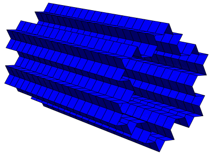
Figure 2. The lateral surface $S_{2}$.

3. A 3D magnetostatics problem

We formulate a linear magnetostatic problem on the fractal domain $Q$. To deduce it and to explain its physical meaning we start by recalling Maxwell’s equations for classical macroscopic electromagnetic fields. We assume that $Q$ is made up from a linear material, i.e. in a material without any magnetization or polarization effects, and we assume it is dielectric, i.e. its conductivity can be neglected, see for instance [Monk03, Section 1.2.1]. Then Ampère’s law, $\operatorname{curl}(\mathcal{H})=\mathcal{J}+\frac{\partial\mathcal{D}}{\partial t}$, tells that the total magnetic field $\mathcal{H}$ induced around a closed loop equals the electric current plus the rate of change of the electric displacement field $\mathcal{D}$ enclosed by the loop, here $\mathcal{J}$ denotes the electric current density, i.e. the vector field describing the directed flow of electric charges. The corresponding magnetic induction is $\mathcal{B}=\mu\mathcal{H}$, where $\mu$ is a positive and bounded scalar function of space and time, called the permeability of the material. By Faraday’s law of induction, $\operatorname{curl}(\mathcal{E})=-\frac{\partial\mathcal{B}}{\partial t}$, the voltage induced in a closed loop equals the change of the enclosed magnetic field. Here $\mathcal{E}=\frac{1}{\varepsilon}\mathcal{D}$, where $\varepsilon$ is a positive and bounded scalar of space and time referred to as the permittivity of the material. These assumptions of $\mu$ and $\varepsilon$ mean we model a inhomogeneous isotropic material, so practically $Q$ may consist of a mixture of different materials whose electromagnetic properties may depend on the location in space but not on the direction of the fields. Gauss’ law, $\operatorname{div}(\mathcal{D})=\rho$, states that the electric flux leaving a volume equals the charge inside, here $\rho\geq 0$ is the charge density. According to Gauss’ law for magnetism, $\operatorname{div}(\mathcal{B})=0$, i.e. the magnetic flux through a closed surface is zero.

We now make the following assumptions leading to a much simpler magnetostatic setup:

• the permittivity $\varepsilon=\varepsilon(x)$ and the permeability $\mu=\mu(x)$ are time-independent;

• the charge density is zero, $\rho=0$;

• the current density $\mathcal{J}\equiv{\bf J}(x)$ is time-independent and real valued;

• the fields $\mathcal{E}\equiv{\bf E}(x)$ and $\mathcal{H}\equiv{\bf H}(x)$ are time-independent and real valued;

• all the fields vanish outside $Q$.

Under these assumptions, Maxwell’s equations on $Q$ read

(3.1) $$\operatorname{curl}(\bf{H})=\bf{J},\quad\operatorname{curl}({\bf E})=0,\quad\operatorname{div}(\bf{D})=0,\quad\operatorname{div}(\bf{B})=0,$$

where ${\bf D}=\varepsilon{\bf E}$ and ${\bf B}=\mu{\bf H}$.

Our assumption that ${\bf E}$ vanishes in $Q^{c}$ means that the surrounding region $Q^{c}$ is a perfect conductor. When passing from one to another medium the parallel component of the electric field should be continuous, this can be seen by taking a small rectangular loop with long sides parallel to $\partial Q$, one inside $Q$, one outside and applying Faraday’s law. Since the field vanishes outside $Q$ this forces to impose what is referred to as the perfectly conducting boundary condition ${\bf n}\times{\bf E}=0$ on $\partial Q$.

Since ${\bf B}$ is divergence free, there exists a magnetic vector potential ${\bf u}=(u_{1},u_{2},u_{3})$ such that ${\bf B}=\operatorname{curl}({\bf u})$, and we may choose it to be divergence free, $\operatorname{div}{\bf u}=0$. Note that Gauss’ law for magnetism then becomes trivial.

Also ${\bf B}$ is supposed to be zero on $Q^{c}$. Therefore, looking at the flux of the magnetic field through small closed loops on $\partial Q$, which should not differ for the interior and the exterior field, and applying the Kelvin-Stokes theorem, it follows that we should impose ${\bf n}\times{\bf u}=0$ on $\partial Q$. See for instance [Griffiths, Section 5.4.2] or [vago, p. 82].

We now restrict attention to the magnetic field only and pose the following problem: Given $\mu$ and ${\bf J}$ as above, find a magnetic vector potential ${\bf u}$ that satisfies

(3.2) $$(P)\begin{cases}\operatorname{curl}\left(\frac{1}{\mu}\operatorname{curl}({\bf u})\right)={\bf J}\quad&\text{in}\,\,Q,\\[5.69054pt] \operatorname{div}{\bf u}=0\quad&\text{in}\,\,Q,\\[5.69054pt] {\bf n}\times{\bf u}=0&\text{on}\,\,\partial Q.\end{cases}$$

Note that if $\mu$ is constant then the first equation rewrites

(3.3) $$-\Delta_{\operatorname{vec}}{\bf u}=\mu{\bf J},$$

where $\Delta_{\operatorname{vec}}$ denotes the vector Laplacian.

4. Trace theorems, Stokes formula and Gauss-Green identity

We discuss measures, function spaces and trace theorems. The latter allow rigorous definitions of boundary conditions and generalizations of classical integral formulas. We write $B(P,r)=\{P^{\prime}\in\mathbb{R}^{N}\,:\,|P^{\prime}-P|<r\}$, $P\in\mathbb{R}^{N},r>0$, for the euclidean ball of radius $r$ centered at $P$. For the two-dimensional Lebesgue measure we write $\mathrm{d}x_{1}\mathrm{d}x_{2}$ and for the three-dimensional one we write $\mathrm{d}x=\mathrm{d}x_{1}\mathrm{d}x_{2}\mathrm{d}x_{3}$.

On the snowflake curve $\displaystyle F=\bigcup_{i=1}^{3}K^{(i)}$ we consider the finite Borel measure $\mu$ defined by

$$\mu_{F}:=\mu_{1}+\mu_{2}+\mu_{3},$$

where $\mu_{i}$ denotes the normalized Hausdorff measure of dimension $D_{f}=\frac{\ln 4}{\ln 3}$, restricted to $K_{i}$, $i=1,2,3$. It is well known that $c_{1}r^{D_{f}}\leq\mu_{F}(B(P,r))\leq c_{2}r^{D_{f}}$, $P\in F$, $r>0$, with positive constants $c_{1}$ and $c_{2}$. If we endow the cylindrical type surface $S=F\times I$ with the measure

$$\mathrm{d}\mu_{S}:=\mathrm{d}\mu_{F}\times\mathrm{d}x_{3},$$

where $\mathrm{d}x_{3}$ is one-dimensional Lebesgue measure on $I$, then clearly

(4.1) $$c_{1}r^{D_{f}+1}\leq\mu_{S}(B(P,r))\leq c_{2}r^{D_{f}+1}$$

for all $P\in S$ and $r>0$.

We equip the boundary $\partial Q$ with the measure

(4.2) $$\mathrm{d}\mu_{\partial Q}=\chi_{S}\mathrm{d}\mu_{S}+\chi_{\tilde{\Omega}}\mathrm{d}x_{1}\mathrm{d}x_{2},$$

where $\tilde{\Omega}=(\Omega\times\{0\})\cup(\Omega\times\{1\})$ is the union of the two bases of the cylinder domain $Q$ in Notation 2.1. In particular, $\operatorname{supp}\mu_{\partial Q}=\partial Q$.

From (4.1) and the quadratic scaling of the two-dimensional Lebesgue measure it follows that

(4.3) $$\mu_{\partial Q}(B(P,kr))\leq c_{1}\>k^{D_{f}+1}\mu_{\partial Q}(B(P,r))\quad\text{and}\quad\mu_{\partial Q}(B(P,kr))\geq c_{2}\>k^{2}\mu_{\partial Q}(B(P,r))$$

for all $P\in\partial Q$, $r>0$, $k\geq 1$ such that $kr\leq 1$.

We write $L^{2}(Q)$ and $L^{2}(Q_{n})$ for the $L^{2}$-spaces with respect to the three-dimensional Lebesgue measure, the spaces $L^{2}(\Omega)$, $L^{2}(\Omega_{n})$, $L^{2}(\partial Q_{n})$ are taken with respect to the two-dimensional Lebesgue respectively Hausdorff measure (depending on whether considered in $\mathbb{R}^{2}$ or $\mathbb{R}^{3}$). For $\partial Q$ we write $L^{2}(\partial Q)=L^{2}(\partial Q,\mu_{\partial Q})$, the $L^{2}$-space with respect to $\mu_{\partial Q}$.

The spaces $H^{\alpha}(\mathbb{R}^{N})=H^{\alpha,2}(\mathbb{R}^{N})$ denote the usual Bessel potential spaces, see for instance [AdHei], where they are denoted by $L^{\alpha,2}(\mathbb{R}^{N})$. Given a domain $O\subset\mathbb{R}^{N}$, the notation $H^{1}(O)$ denotes the classical Sobolev space of square integrable functions with finite Dirichlet integral, usually denoted by $W^{1,2}(O)$.

Since the boundary $\partial Q=\tilde{\Omega}\cup S$ is a closed set composed by sets of different Hausdorff dimension, in order to consider the trace space of $H^{\alpha}(Q)$ on $\partial Q$, we introduce suitable spaces $\tilde{B}_{\alpha}^{2,2}(\partial Q)$ as in [jonsson91, page 356]. For any

(4.4) $$\frac{1}{2}<\alpha<2-\frac{D_{f}}{2}$$

let $\tilde{B}^{2,2}_{\alpha}(\partial Q)$ denote the class of functions $u$ on $\partial Q$ such that

(4.5) $$\|u\|^{2}_{\tilde{B}^{2,2}_{\alpha}(\partial Q)}=\|u\|^{2}_{L^{2}(\partial Q)}+\iint_{|x-y|<1}\frac{|u(x)-u(y)|^{2}}{|x-y|^{2\alpha-3}(\mu_{\partial Q}(B(x,|x-y|)))^{2}}\,\mathrm{d}\mu_{\partial Q}(x)\,\mathrm{d}\mu_{\partial Q}(y)$$

is finite.

We remark that $\mu_{\partial Q}$ defined in (4.2) is not an Ahlfors regular $d$-measure on $\partial Q$. That is, the $\mu_{\partial\Omega}$-measure of a ball of radius $r>0$ can not be estimated from above and below, respectively, by a constant times $r^{d}$. Therefore the space $\tilde{B}^{2,2}_{\alpha}(\partial Q)$ does not coincide with the usual Besov space $B^{2,2}_{\alpha}(\partial Q)$ defined in [JoWa, page 103] or [triebel].

We denote by $|A|$ the Lebesgue measure of a subset $A\subset\mathbb{R}^{N}$. For $f\in H^{\alpha}(O)$, $O\subset\mathbb{R}^{N}$ open, we put

(4.6) $$\gamma_{0}f(P)=\lim_{r\to 0}{1\over|B(P,r)\cap O|}\int_{B(P,r)\cap O}f(x)\,\mathrm{d}x$$

at every point $P\in\overline{O}$ where the limit exists. This is a typical form of restriction operator in the spirit of Lebesgue differentiation.

The following trace theorem is a special case of [jonsson91, Theorem 1], see also [jonsson91, Proposition 2].

Proposition 4.1.

Let $\alpha$ be as in (4.4). $\tilde{B}_{\alpha}^{2,2}(\partial Q)$ is the trace space of $H^{\alpha}(\mathbb{R}^{3})$, that is:

1. $f\mapsto\gamma_{0}f$ is a linear and continuous operator from $H^{\alpha}(\mathbb{R}^{3})$ to $\tilde{B}_{\alpha}^{2,2}(\partial Q)$;

2. There exists a linear and continuous operator ${\hbox{\rm Ext}}\colon\tilde{B}_{\alpha}^{2,2}(\partial Q)\to H^{\alpha}(\mathbb{R}^{3})$ such that $\gamma_{0}\circ{\hbox{\rm Ext}}$ is the identity operator on $\tilde{B}_{\alpha}^{2,2}(\partial Q)$.

Combined with trace and extension results between the spaces $H^{1}(\mathbb{R}^{3})$ and $H^{1}(Q)$, such as for instance [JoWa, Chapter VII, Theorem 1, combined with Chapter VIII, Proposition 1], we obtain the following.

Corollary 4.2.

The space $\tilde{B}_{1}^{2,2}(\partial Q)$ is the trace space of $H^{1}(Q)$ on $\partial Q$, i.e. there exist a continuous linear restriction operator from $H^{1}(Q)$ to $\tilde{B}_{1}^{2,2}(\partial Q)$ and a continuous linear extension from $\tilde{B}_{1}^{2,2}(\partial Q)$ to $H^{1}(Q)$.

For the restriction to $\partial Q$ of a function $f\in H^{1}(Q)$ we write $f|_{\partial Q}$.

More classical trace and extension results cover the case of Lipschitz boundaries, such as the sets $\partial Q_{n}:=S_{n}\cup\tilde{\Omega}_{n}$, where $\tilde{\Omega}_{n}:=(\Omega_{n}\times\left\{0\right\})\cup(\Omega_{n}\times\left\{1\right\})$. For the following result see [grisvard-fr, necas].

Proposition 4.3.

The space $H^{\frac{1}{2}}(\partial Q_{n})$ is the trace space of $H^{1}(Q_{n})$ on $\partial Q_{n}$ in the following sense:

1. $\gamma_{0}$ is a continuous and linear operator from $H^{1}(Q_{n})$ to $H^{\frac{1}{2}}(\partial Q_{n})$;

2. there is a continuous linear operator Ext from $H^{\frac{1}{2}}(\partial Q_{n})$ to $H^{1}(Q_{n})$ such that $\gamma_{0}\circ{\hbox{\rm Ext}}$ is the identity operator in $H^{\frac{1}{2}}(\partial Q_{n})$.

As usual, we write $H^{-\frac{1}{2}}(\partial Q_{n})$ to denote the dual space of $H^{\frac{1}{2}}(\partial Q_{n})$, see [GirRav86, p. 8].

We pass to vector valued functions. Consider the space

$$H(\operatorname{curl},Q):=\left\{{\bf u}=(u_{1},u_{2},u_{3})\colon Q\to\mathbb{R}^{3}:u_{1},u_{2},u_{3}\in L^{2}(Q)\,\,\text{and}\,\operatorname{curl}{\bf u}\in L^{2}(Q)^{3}\right\}.$$

Endowed with the norm $\|{\bf u}\|_{\operatorname{curl},Q}=\left(\left\|{\bf u}\right\|_{L^{2}(Q)^{3}}^{2}+\left\|\operatorname{curl}{\bf u}\right\|^{2}_{L^{2}(Q)^{3}}\right)^{1/2}$, it becomes a Hilbert space, see for instance [duv-lions, GirRav86] or [temam].

We now prove a generalized vector Stokes formula. Suppose ${\bf{u}}\in H(\operatorname{curl},Q)$. For any ${\bf v}\in\tilde{B}^{2,2}_{1}(\partial Q)^{3}$ let ${\bf w}\in H^{1}(Q)^{3}$ be such that ${\bf w}|_{\partial Q}={\bf v}$, defined component-wise in the sense of Corollary 4.2, and consider the quantity

$$\gamma_{\tau}{\bf u}({\bf{v}}):=\int_{Q}{\bf{u}}\cdot\operatorname{curl}\,{\bf{w}}\,\mathrm{d}x-\int_{Q}{\bf{w}}\cdot\operatorname{curl}\,{\bf{u}}\,\mathrm{d}x.$$

Theorem 4.4.

Let $Q$ be the Koch-type pipe.

1. The map ${\bf u}\mapsto\gamma_{\tau}\bf{u}$ is well defined as a bounded linear operator from $H(\operatorname{curl},Q)$ into $((\tilde{B}^{2,2}_{1}(\partial Q))^{\prime})^{3}$. By setting ${\bf{u}}\times{\bf{n}}|_{\partial Q}:=\gamma_{\tau}\bf{u}$ we have

   (4.7) $$|\left\langle{\bf{u}\times\bf{n}}|_{\partial Q},{\bf{v}}\right\rangle_{((\tilde{B}^{2,2}_{1}(\partial Q))^{\prime})^{3},\tilde{B}^{2,2}_{1}(\partial Q)^{3}}|\leq c\left\|{\bf{u}}\right\|_{\operatorname{curl},Q}\left\|{\bf{v}}\right\|_{\tilde{B}^{2,2}_{1}(\partial Q)^{3}}$$

   for all ${\bf u}\in H(\operatorname{curl},Q)$ and ${\bf v}\in\tilde{B}^{2,2}_{1}(\partial Q)^{3}$.

2. Moreover, we have

   (4.8) $$\left\langle{\bf{u}}\times{\bf{n}}|_{\partial Q},{\bf w}|_{\partial Q}\right\rangle_{((\tilde{B}^{2,2}_{1}(\partial Q))^{\prime})^{3},\tilde{B}^{2,2}_{1}(\partial Q)^{3}}=\lim_{n\to\infty}\left\langle{\bf u}\times{\bf n}|_{\partial Q_{n}},{\bf{w}}|_{\partial Q_{n}}\right\rangle_{H^{-\frac{1}{2}}(\partial Q_{n})^{3},H^{\frac{1}{2}}(\partial Q_{n})^{3}}$$

   and

   (4.9) $$\left\langle{\bf{u}}\times{\bf{n}}|_{\partial Q},{\bf w}|_{\partial Q}\right\rangle_{((\tilde{B}^{2,2}_{1}(\partial Q))^{\prime})^{3},\tilde{B}^{2,2}_{1}(\partial Q)^{3}}=\int_{Q}{\bf u}\cdot\operatorname{curl}{\bf{w}}\,\mathrm{d}x-\int_{Q}{\bf{w}}\cdot\operatorname{curl}{\bf u}\,\mathrm{d}x$$

   for all ${\bf u}\in H(\operatorname{curl},Q)$ and ${\bf{w}}\in H^{1}(Q)^{3}$.

Formula (4.8) provides a suitable approximation of ${\bf{u}}\times{\bf{n}}|_{\partial Q}$ in terms of the tangential traces ${\bf u}\times{\bf n}|_{\partial Q_{n}}$ along the Lipschitz boundaries $\partial Q_{n}$, see [GirRav86, §2, Theorem 2.11] or [temam]. In this sense ${\bf u}\times{\bf n}|_{\partial Q}$ can be seen as a generalized tangential trace and (4.9) is a generalized Stokes formula.

Proof.

Let ${\bf u}\in H(\operatorname{curl},Q)$. Given ${\bf v}\in\tilde{B}^{2,2}_{1}(\partial Q)^{3}$, let ${\bf{w}}\in H^{1}(Q)^{3}$ be such that ${\bf w}|_{\partial Q}={\bf v}$ in $\tilde{B}^{2,2}_{1}(\partial Q)^{3}$. Then Cauchy-Schwarz together with the inclusion $H^{1}(Q)^{3}\subset H(\operatorname{curl},Q)$ and Corollary 4.2 lead to the estimate

$$|\left\langle{\bf{u}}\times{\bf{n}}|_{\partial Q},{\bf w}|_{\partial Q}\right\rangle| \leq\|{\bf u}\|_{L^{2}(Q)^{3}}\|\operatorname{curl}{\bf{w}}\|_{L^{2}(Q)^{3}}+\|{\bf{w}}\|_{L^{2}(Q)^{3}}\|{\bf\operatorname{curl}u}\|_{L^{2}(Q)^{3}}$$

$$\leq c\,\|{\bf w}\|_{H^{1}(Q)^{3}}\|{\bf u}\|_{\operatorname{curl},Q}$$

$$\leq c\,\|{\bf v}\|_{\tilde{B}^{2,2}_{1}(\partial Q)^{3}}\|{\bf u}\|_{\operatorname{curl},Q}.$$

This shows in particular, that $\gamma_{\tau}{\bf u}({\bf{v}})$ is independent from the choice of the extension ${\bf w}$ of ${\bf v}$, and that $\bf{u}\times\bf{n}$ is an element of $((\tilde{B}^{2,2}_{1}(\partial Q))^{\prime})^{3}$ which satisfies (4.7).

We now consider the sequence of domains $Q_{n}=\Omega_{n}\times I$, which are bounded Lipschitz domains and satisfy $Q_{n}\subset Q_{n+1}$ and $Q=\bigcup_{n=1}^{\infty}Q_{n}$. By the vector Stokes formula for Lipschitz domains, cf. [GirRav86, §2, Theorem 2.11] or Appendix I in [temam], together with the dominated convergence theorem, we have

$$\lim_{n\to\infty}\left\langle{\bf u}\times{\bf n}|_{\partial Q_{n}},{\bf{w}}|_{\partial Q_{n}}\right\rangle_{H^{-\frac{1}{2}}(\partial Q_{n})^{3},H^{\frac{1}{2}}(\partial Q_{n})^{3}} =\lim_{n\to\infty}\int_{Q_{n}}{\bf u}\cdot\operatorname{curl}{\bf{w}}\,\mathrm{d}x-\int_{Q_{n}}{\bf{w}}\cdot\operatorname{curl}{\bf u}\,\mathrm{d}x$$

$$=\int_{Q}{\bf u}\cdot\operatorname{curl}{\bf{w}}\,\mathrm{d}x-\int_{Q}{\bf{w}}\cdot\operatorname{curl}{\bf u}\,\mathrm{d}x$$

$$=\left\langle{\bf{u}\times\bf{n}},{\bf w}|_{\partial Q}\right\rangle_{((\tilde{B}^{2,2}_{1}(\partial Q))^{\prime})^{3},\tilde{B}^{2,2}_{1}(\partial Q)^{3}}$$

for all ${\bf{w}}\in H^{1}(Q)^{3}$ and $n$, where ${\bf u}\times{\bf n}|_{\partial Q_{n}}$ is defined as an element of $H^{-\frac{1}{2}}(\partial Q_{n})^{3}$. ∎

Next, consider the space

$$H(\operatorname{div},Q):=\left\{{\bf u}=(u_{1},u_{2},u_{3})\colon Q\to\mathbb{R}^{3}:u_{1},u_{2},u_{3}\in L^{2}(Q)\,\,\text{and}\,\operatorname{div}{\bf u}\in L^{2}(Q)\right\},$$

which is Hilbert when equipped with the norm $\|{\bf u}\|_{\operatorname{div},Q}=\left(\left\|{\bf u}\right\|_{L^{2}(Q)^{3}}^{2}+\left\|\operatorname{div}{\bf u}\right\|^{2}_{L^{2}(Q)}\right)^{1/2}$. Following the same pattern as above one can establish a generalized Gauss-Green formula. This can be done as in [LaVe2].

Suppose ${\bf u}\in H(\operatorname{div},Q)$. For any $v\in\tilde{B}^{2,2}_{1}(\partial Q)$ let $w\in H^{1}(Q)$ be such that $w|_{\partial Q}=v$ in the sense of Corollary 4.2 and consider

$$\gamma_{\nu}{\bf u}(v):=\int_{Q}{\bf u}\cdot\nabla w\>\mathrm{d}x+\int_{Q}(\operatorname{div}{\bf u})w\>\mathrm{d}x.$$

By proceeding as in [LaVe2, Theorem 3.7] we can prove the following Green formula.