Petrov-Galerkin Method for Fully Distributed-Order
Fractional Partial Differential Equations

Abstract

Distributed-order PDEs are tractable mathematical models for complex multiscaling anomalous transport, where derivative orders are distributed over a range of values. We develop a fast and stable Petrov-Galerkin spectral method for such models by employing Jacobi poly-fractonomials and Legendre polynomials as temporal and spatial basis/test functions, respectively. By defining the proper underlying distributed Sobolev spaces and their equivalent norms, we prove the well-posedness of the weak formulation, and thereby carry out the corresponding stability and error analysis. We finally provide several numerical simulations to study the performance and convergence of proposed scheme.

1 Introduction

Over the past decades, anomalous transport has been observed and investigated in a wide range of applications such as turbulence [51, 42, 20, 10], porous media [56, 4, 63, 15, 62, 6], geoscience [5], bioscience [44, 45, 46, 47], and viscoelastic material [53, 19, 39]. The underlying anomalous features, manifesting in memory-effects, non-local interactions, power-law distributions, sharp peaks, and self-similar structures, can be well-described by fractional partial differential equations (FPDEs) [40, 41, 26, 43]. However, in cases where a single power-law scaling is not observed over the whole domain, the processes cannot be characterized by a fixed fractional order [52]. Examples include accelerating superdiffusion, decelerating subdiffusion [18, 52], and random processes subordinated to Wiener processes [13, 27, 41, 14, 36, 35, 7]. A faithful description of such anomalous transport requires exploiting distributed-order derivatives, in which the derivative order has a distribution over a range of values.

Numerical methods for FPDEs, which can exhibit history dependence and non-local features have been recently addressed by developing finite-element methods [22, 2], spectral/spectral-element methods [57, 9, 37, 48, 38, 25], and also finite-difference and finite-volume methods [11, 33, 3]. Distributed-order FPDEs impose further complications in numerical analysis by introducing distribution functions, which require compliant underlying function spaces, as well as efficient and accurate integration techniques over the order of the fractional derivatives. In [58, 28, 17, 54, 32, 21], numerical analysis of distributed-order FPDEs was extensively investigated. More recently, Liao et al. [31] studied simulation of a distributed subdiffusion equation, approximating the distributed order Caputo derivative using piecewise-linear and quadratic interpolating polynomials. Abbaszadeh and Dehghan [1] employed an alternating direction implicit approach, combined with an interpolating element-free Galerkin method, on distributed-order time-fractional diffusion-wave equations. Kharazmi and Zayernouri [23] developed a pseudo-spectral method of Petrov-Galerkin sense, employing nodal expansions in the weak formulation of distributed-order fractional PDEs. In [24], they also introduced distributed Sobolev space and developed two spectrally accurate schemes, namely, a Petrov–Galerkin spectral method and a spectral collocation method for distributed order fractional differential equations. Besides, Tomovski and Sandev [55] investigated the solution of generalized distributed-order diffusion equations with fractional time-derivative, using the Fourier-Laplace transform method.

The main purpose of this study is to develop and analyze a Petrov-Galerkin (PG) spectral method to solve a $(1+d)$-dimensional fully distributed-order FPDE with two-sided derivatives of the form

$$\int_{\tau^{min}}^{\tau^{max}}\varphi(\tau)\,\prescript{C}{0}{\mathcal{D}}_{t}^{2\tau}u\,\,d\tau+\sum_{i=1}^{d}\int_{\mu_{i}^{min}}^{\mu_{i}^{max}}\varrho_{i}(\mu_{i})\,[c_{l_{i}}\prescript{RL}{a_{i}}{\mathcal{D}}_{x_{i}}^{2\mu_{i}}u+c_{r_{i}}\prescript{RL}{x_{i}}{\mathcal{D}}_{b_{i}}^{2\mu_{i}}u]\,\,d\mu_{i}$$

(1.1) $$=\sum_{j=1}^{d}\int_{\nu_{j}^{min}}^{\nu_{j}^{max}}\rho_{j}(\nu_{j})\,[\kappa_{l_{j}}\prescript{RL}{a_{j}}{\mathcal{D}}_{x_{j}}^{2\nu_{j}}u+\kappa_{r_{j}}\prescript{RL}{x_{j}}{\mathcal{D}}_{b_{j}}^{2\nu_{j}}u]\,\,d\nu_{j}-\gamma\,\,u+f,$$

subject to homogeneous Dirichlet boundary conditions and zero initial condition, where for $i,j=1,\,2,\,...,\,d$

$$t\in[0,\,T],\quad x_{j}\in[a_{j},\,b_{j}],$$

$$2\tau^{min}<2\tau^{max}\,\in(0,\,2],\,\,2\tau^{min}\neq 1,\,\,2\tau^{max}\neq 1,$$

$$2\mu_{i}^{min}<2\mu_{i}^{max}\,\in(0,\,1],\,\,2\nu_{j}^{min}<2\nu_{j}^{max}\,\in(1,\,2],$$

$$0<\varphi(\tau)\in L^{1}((\tau^{min},\tau^{max})),\,\,0<\varrho_{i}(\mu_{i})\in L^{1}((\mu_{i}^{min},\mu_{i}^{max})),\,\,0<\rho_{j}(\nu_{j})\in L^{1}((\nu_{j}^{min},\nu_{j}^{max})),$$

and the coefficients $c_{l_{i}}$, $c_{r_{i}}$, $\kappa_{l_{i}}$, $\kappa_{r_{i}}$, and $\gamma$ are constant. We briefly highlight the main contributions of this study as follows.

• We consider fully distributed fractional PDEs as an extension of the existing fractional PDEs in [48, 24] by replacing the fractional operators by their corresponding distributed order ones. We further derive the weak formulation of the problem.

• We construct the underlying function spaces by extending the distributed Sobolev space in [24] to higher dimensions in time and space, endowed with equivalent associated norms.

• We develop a Petrov-Galerkin spectral method, employing Legendre polynomials and Jacobi poly-fractonomials [61] as spatial and temporal basis/test functions, respectively. We also formulate a fast solver for the corresponding weak form of (1), following [48], which significantly reduces the computational expenses in high-dimensional problems.

• We establish well-posedness of the weak form of the problem in the underlying distributed Sobolev spaces respecting the analysis in [49] and prove the stability of the proposed numerical scheme. We additionally perform the corresponding error analysis, where the distributed Sobolev spaces enable us to obtain accurate error estimate of the scheme.

We note that the model (1) includes distributed-order fractional diffusion and fractional advection-dispersion equations (FADEs) with constant coefficients on bounded domains, when the corresponding distributions $\varphi$, $\varrho_{i}$, and $\varrho_{j}$, $i,j=1,2,\cdots,d$ are chosen to be Dirac delta functions. To examine the performance and convergence of the developed PG method in solving different cases, we also perform several numerical simulations.

The paper is organized as follows: in Section 2, we introduce some preliminaries from fractional calculus. In Section 3, we present the mathematical framework of the bilinear form and carry out the corresponding well-posedness analysis. We construct the PG method for the discrete weak form problem and formulate the fast solver in Section 4. In Section 5, we perform the stability and error analysis in detail. In Section 6, we illustrate the convergence rate and the efficiency of method via numerical examples. We conclude the paper with a summary.

2 Preliminaries on Fractional Calculus

Recalling the definitions of the fractional derivatives and integrals from [61, 41], we denote by $\prescript{RL}{a}{\mathcal{D}}_{x}^{\sigma}g(x)$ and $\prescript{RL}{x}{\mathcal{D}}_{b}^{\sigma}g(x)$ the left-sided and the right-sided Reimann-Liouville fractional derivatives of order $\sigma>0$,

(2.1) $$\prescript{RL}{a}{\mathcal{D}}_{x}^{\sigma}g(x)=\frac{1}{\Gamma(n-\sigma)}\frac{d^{n}}{dx^{n}}\int_{a}^{x}\frac{g(s)}{(x-s)^{\sigma+1-n}}\,\,ds,\quad x\in[a,b],$$

(2.2) $$\prescript{RL}{x}{\mathcal{D}}_{b}^{\sigma}g(x)=\frac{(-1)^{n}}{\Gamma(n-\sigma)}\frac{d^{n}}{dx^{n}}\int_{x}^{b}\frac{g(s)}{(s-x)^{\sigma+1-n}}\,\,ds,\quad x\in[a,b],$$

in which $g(x)\in L^{1}[a,b]$ and $\int_{a}^{x}\frac{g(s)}{(x-s)^{\sigma+1-n}}\,\,ds,\,\,\int_{a}^{x}\frac{g(s)}{(x-s)^{\sigma+1-n}}\,\,ds\in C^{n}[a,b]$, respectively, where $n=\lceil\sigma\rceil$. Besides, $\prescript{C}{a}{\mathcal{D}}_{x}^{\sigma}g(x)$ and $\prescript{C}{x}{\mathcal{D}}_{b}^{\sigma}g(x)$ represent the left-sided and the right-sided Caputo fractional derivatives, where

(2.3) $$\prescript{C}{a}{\mathcal{D}}_{x}^{\sigma}f(x)\,=\,\frac{1}{\Gamma(n-\nu)}\int_{a}^{x}\frac{g^{(n)}(s)}{(x-s)^{\nu+1-n}}\,\,ds,\quad x\in[a,b],$$

(2.4) $$\prescript{C}{x}{\mathcal{D}}_{b}^{\sigma}f(x)\,=\,\frac{(-1)^{n}}{\Gamma(n-\nu)}\int_{x}^{b}\frac{g^{(n)}(s)}{(s-x)^{\nu+1-n}}\,\,ds,\quad x\in[a,b].$$

The relationship between the RL and the Caputo fractional derivatives is given by

(2.5) $$\prescript{Rl}{a}{\mathcal{D}}_{x}^{\nu}f(x)\,=\,\frac{f(a)}{\Gamma(1-\nu)(x-a)^{\nu}}\,+\,\prescript{C}{a}{\mathcal{D}}_{x}^{\nu}f(x)$$

(2.6) $$\prescript{Rl}{x}{\mathcal{D}}_{b}^{\nu}f(x)\,=\,\frac{f(b)}{\Gamma(1-\nu)(b-x)^{\nu}}\,+\,\prescript{C}{x}{\mathcal{D}}_{b}^{\nu}f(x),$$

when $\lceil\nu\rceil=1$, see e.g. (2.33) in [41]. In the case of homogeneous boundary conditions, we obtain $\prescript{Rl}{a}{\mathcal{D}}_{x}^{\nu}f(x)=\prescript{C}{a}{\mathcal{D}}_{x}^{\nu}f(x):=\prescript{}{a}{\mathcal{D}}_{x}^{\nu}f(x)$ and $\prescript{Rl}{x}{\mathcal{D}}_{b}^{\nu}f(x)=\prescript{C}{x}{\mathcal{D}}_{b}^{\nu}f(x):=\prescript{}{x}{\mathcal{D}}_{b}^{\nu}f(x)$. The Reimann-Liouville fractional integrals of Jacobi poly-fractonomials are analytically obtained in the standard domain $\xi\in[-1,1]$ as [61, 60]

(2.7) $$\prescript{RL}{-1}{\mathcal{I}}_{\xi}^{\sigma}\{(1+\xi)^{\beta}P_{n}^{\alpha,\beta}{(\xi)}\}=\frac{\Gamma(n+\beta+1)}{\Gamma(n+\beta+\sigma+1)}\,(1+\xi)^{\beta+\sigma}P_{n}^{\alpha-\sigma,\beta+\sigma}{(\xi)},$$

and

(2.8) $$\prescript{RL}{\xi}{\mathcal{I}}_{1}^{\sigma}\{(1-\xi)^{\alpha}P_{n}^{\alpha,\beta}{(\xi)}\}=\frac{\Gamma(n+\alpha+1)}{\Gamma(n+\alpha+\sigma+1)}\,(1-\xi)^{\alpha+\sigma}P_{n}^{\alpha+\sigma,\beta-\sigma}{(\xi)},$$

where $0<\sigma<1$, $\alpha>-1$, $\beta>-1$, and $P^{\alpha,\,\beta}_{n}(\xi)$ denotes the standard Jacobi polynomials of order $n$ and parameters $\alpha$ and $\beta$ [8]. Accordingly,

(2.9) $$\prescript{RL}{-1}{\mathcal{D}}_{\xi}^{\sigma}P_{n}(\xi)=\frac{\Gamma(n+1)}{\Gamma(n-\sigma+1)}P_{n}^{\,\sigma,-\sigma}{(\xi)}\,(1+\xi)^{-\sigma}$$

and

(2.10) $$\prescript{RL}{\xi}{\mathcal{D}}_{1}^{\sigma}P_{n}(\xi)=\frac{\Gamma(n+1)}{\Gamma(n-\sigma+1)}P_{n}^{\,-\sigma,\sigma}{(\xi)}\,(1-\xi)^{-\sigma},\,$$

where $P_{n}(\xi):=P^{\,0,0}_{n}(\xi)$ represents Legendre polynomial of degree $n$ (see [8]).

Let define the distributed-order derivative as

(2.11) $$\prescript{D}{}{\mathcal{D}}_{t}^{\phi}f(t,x):=\int_{\tau^{min}}^{\tau^{max}}\phi(\tau)\prescript{}{0}{\mathcal{D}}_{t}^{\tau}f(t,x)d\tau,$$

where $\alpha\rightarrow\phi(\alpha)$ be a continuous mapping in $[\alpha_{min},\alpha_{max}]$ [24] and $t>0$. We note that by choosing the distribution function in the distributed-order derivatives to be the Dirac delta function $\delta(\tau-\tau_{0})$, we recover a single (fixed) term fractional derivative, i.e.,

(2.12) $$\int_{\tau^{min}}^{\tau^{max}}\delta(\tau-\tau_{0})\prescript{}{0}{\mathcal{D}}_{t}^{\tau}f(t,x)d\tau=\prescript{}{0}{\mathcal{D}}_{t}^{\tau_{0}}f(t,x),$$

where $\tau_{0}\in(\tau_{min},\tau_{max})$.

3 Mathematical Formulation

We introduce the underlying solution and test spaces along with their proper norms, and also provide some useful lemmas to derive the corresponding bilinear form and thus, prove the well-posedness of the problem.

3.1 Mathematical Framework

Recalling the definition of Sobolev space for real $s\geq 0$ from [24, 29], the usual Sobolev space, denoted by $H^{s}(I)$ on the finite interval $I=(0,T)$, is associated with the norm $\|\cdot\|_{H^{s}(I)}$. According to [29, 16],

(3.1) $$|\cdot|_{H^{s}(I)}\cong|\cdot|_{{{}^{l}}H^{s}(I)}\cong|\cdot|_{{{}^{r}}H^{s}(I)}$$

where $"\cong"$ denotes equivalence relation, $|\cdot|_{{{}^{l}}H^{s}(I)}=\|\prescript{}{0}{\mathcal{D}}_{t}^{s}(\cdot)\|_{L^{2}(I)}$, and $|\cdot|_{{{}^{r}}H^{s}(I)}=\|\prescript{}{t}{\mathcal{D}}_{T}^{s}(\cdot)\|_{L^{2}(I)}$. Take $\Lambda=(a,b)$. For the real index $\sigma\geq 0$ and $\sigma\neq n-\frac{1}{2}$ on the bounded interval $\Lambda$ the following norms are equivalent [30]

(3.2) $$\|\cdot\|_{H^{\sigma}(\Lambda)}\cong\|\cdot\|_{{{}^{l}}H^{\sigma}(\Lambda)}\cong\|\cdot\|_{{{}^{r}}H^{\sigma}(\Lambda)}\cong|\cdot|_{{}H^{\sigma}(\Lambda)}^{*},$$

where $\|\cdot\|_{{{}^{l}}H^{\sigma}(\Lambda)}=\Big{(}\|\prescript{}{a}{\mathcal{D}}_{x}^{\sigma}\,(\cdot)\|_{L^{2}(\Lambda)}^{2}+\|\cdot\|_{L^{2}(\Lambda)}^{2}\Big{)}^{\frac{1}{2}}$, $\|\cdot\|_{{{}^{r}}H^{\sigma}(\Lambda)}=\Big{(}\|\prescript{}{x}{\mathcal{D}}_{b}^{\sigma}\,(\cdot)\|_{L^{2}(\Lambda)}^{2}+\|\cdot\|_{L^{2}(\Lambda)}^{2}\Big{)}^{\frac{1}{2}},$ and $|\cdot|_{{{}^{l}}H^{\sigma}(I)}^{*}=|(\prescript{}{0}{\mathcal{D}}_{t}^{\sigma}(\cdot),\prescript{}{t}{\mathcal{D}}_{T}^{\sigma}(\cdot))_{I}|^{\frac{1}{2}}$. From Lemma 5.2 in [16], we have

(3.3) $$|\cdot|_{{{}^{l}}H^{\sigma}(I)}^{*}\cong|\cdot|_{{{}^{l}}H^{\sigma}(I)}^{\frac{1}{2}}\,|\cdot|_{{{}^{r}}H^{\sigma}(I)}^{\frac{1}{2}}=\|\prescript{}{0}{\mathcal{D}}_{t}^{\sigma}(\cdot)\|_{L^{2}(I)}^{\frac{1}{2}}\,\|\prescript{}{t}{\mathcal{D}}_{T}^{\sigma}(\cdot)\|_{L^{2}(I)}^{\frac{1}{2}}.$$

Let $C_{0}^{\infty}(\Lambda)$ represent the space of smooth functions with compact support in $\Lambda$. According to Lemma 3.1 in [49], the norms $\|\cdot\|_{{{}^{l}}H^{\sigma}(\Lambda)}$ and $\|\cdot\|_{{{}^{r}}H^{\sigma}(\Lambda)}$ are equivalent to $\|\cdot\|_{{{}^{c}}H^{\sigma}(\Lambda)}$ in space $C^{\infty}_{0}(\Lambda)$, where

(3.4) $$\|\cdot\|_{{{}^{c}}H^{\sigma}(\Lambda)}=\Big{(}\|\prescript{}{x}{\mathcal{D}}_{b}^{\sigma}\,(\cdot)\|_{L^{2}(\Lambda)}^{2}+\|\prescript{}{a}{\mathcal{D}}_{x}^{\sigma}\,(\cdot)\|_{L^{2}(\Lambda)}^{2}+\|\cdot\|_{L^{2}(\Lambda)}^{2}\Big{)}^{\frac{1}{2}}.$$

In the usual Sobolev space, for $u\in{}H^{\sigma}(\Lambda)$ we define

$$|u|_{{}H^{\sigma}(\Lambda)}^{*}=|(\prescript{}{a}{\mathcal{D}}_{x}^{\sigma}\,u,\prescript{}{x}{\mathcal{D}}_{b}^{\sigma}\,v)_{\Lambda}|^{\frac{1}{2}}+|(\prescript{}{x}{\mathcal{D}}_{b}^{\sigma}\,u,\prescript{}{a}{\mathcal{D}}_{x}^{\sigma}\,v)_{\Lambda}|^{\frac{1}{2}},\quad\forall v\in{}H^{\sigma}(\Lambda),$$

assuming $\underset{u\in H^{\sigma}(\Lambda)}{\sup}|(\prescript{}{a}{\mathcal{D}}_{x}^{\sigma}\,u,\prescript{}{x}{\mathcal{D}}_{b}^{\sigma}\,v)_{\Lambda}|^{\frac{1}{2}}+|(\prescript{}{x}{\mathcal{D}}_{b}^{\sigma}\,u,\prescript{}{a}{\mathcal{D}}_{x}^{\sigma}\,v)_{\Lambda}|^{\frac{1}{2}}>0\quad\forall v\in H^{\sigma}(\Lambda)$. Denoted by ${{}^{l}}H^{\sigma}_{0}(\Lambda)$ and ${{}^{r}}H^{\sigma}_{0}(\Lambda)$ are the closure of $C^{\infty}_{0}(\Lambda)$ with respect to the norms $\|\cdot\|_{{{}^{l}}H^{\sigma}(\Lambda)}$ and $\|\cdot\|_{{{}^{r}}H^{\sigma}(\Lambda)}$in $\Lambda$, respectively, where $C^{\infty}_{0}(\Lambda)$ is the space of smooth functions with compact support in $\Lambda$.

Recalling from [24], ${{}^{\mathfrak{D}}}H^{\varphi}(\mathbb{R})$ represents the distributed Sobolev space on $\mathbb{R}$ , which is associated with the following norm

(3.5) $$\|\cdot\|_{{{}^{\mathfrak{D}}}H^{\varphi}(\mathbb{R})}=\left(\int_{\tau^{min}}^{\tau^{max}}\varphi(\tau)\,\,\|\,(1+|\omega|^{2})^{\frac{\tau}{2}}\mathcal{F}(\cdot)(\omega)\|^{2}_{L^{2}(\mathbb{R})}\,\,d\tau\right)^{\frac{1}{2}},$$

where $0<\varphi(\tau)\in L^{1}(\,[\tau^{min},\tau^{max}]\,)$, $0\leq\tau^{min}<\tau^{max}$. Subsequently, we denote by ${{}^{\mathfrak{D}}}H^{\varphi}(I)$ the distributed Sobolev space on the bounded open interval $I=(0,T)$, which is defined as ${{}^{\mathfrak{D}}}H^{\varphi}(I)=\{v\in L^{2}(I)|\,\,\,\exists\tilde{v}\in{{}^{\mathfrak{D}}}H^{\varphi}(\mathbb{R})\,\,\,s.t.\,\,\,\tilde{v}|_{I}=v\}$ with the the equivalent norms $\|\cdot\|_{{{}^{l,\mathfrak{D}}}H^{\varphi}(I)}$ and $\|\cdot\|_{{{}^{r,\mathfrak{D}}}H^{\varphi}(I)}$ in [24], where

$$\|\cdot\|_{{{}^{l,\mathfrak{D}}}H^{\varphi}(I)}=\left(\|\cdot\|^{2}_{L^{2}(I)}+\int_{\tau^{min}}^{\tau^{max}}\varphi(\tau)\,\,\|\,\prescript{}{0}{\mathcal{D}}_{t}^{\tau}(\cdot)\|^{2}_{L^{2}(I)}\,\,d\tau\right)^{\frac{1}{2}},$$

and

$$\|\cdot\|_{{}^{r,\mathfrak{D}}H^{\varphi}(I)}=\left(\|\cdot\|^{2}_{L^{2}(I)}+\int_{\tau^{min}}^{\tau^{max}}\varphi(\tau)\,\,\|\,\prescript{}{t}{\mathcal{D}}_{T}^{\tau}(\cdot)\|^{2}_{L^{2}(I)}\,\,d\tau\right)^{\frac{1}{2}}.$$

In each realization of a physical process (e.g., sub- or super-diffusion) the distribution function $\varphi(\tau)$ can be obtained from experimental observations, while the theoretical setting of the problem remains invariant. More importantly, choice of distributed Sobolev space and the associated norms provide a sharper estimate for the accuracy of the proposed PG method.

Let $\Lambda_{1}=(a_{1},b_{1})$, $\Lambda_{i}=(a_{i},b_{i})\times\Lambda_{i-1}$ for $i=2,\cdots,d$. We define $\mathcal{X}_{1}={{}^{\mathfrak{D}}}H^{\rho_{1}}(\Lambda_{1})$ with the associated norm $\|\cdot\|_{{{}^{\mathfrak{D}}}H^{\rho_{1}}(\Lambda_{1})}$, where

(3.6) $$\|\cdot\|_{{{}^{\mathfrak{D}}}H^{\rho_{1}}(\Lambda_{1})}=\left(\|\cdot\|^{2}_{L^{2}(I)}+\int_{\nu^{min}_{1}}^{\nu^{max}_{1}}\rho_{1}(\nu_{1})\,\left(\|\,\prescript{}{a_{1}}{\mathcal{D}}_{x_{1}}^{\nu_{1}}(\cdot)\|^{2}_{L^{2}(\Lambda_{1})}+\|\prescript{}{x_{1}}{\mathcal{D}}_{b_{1}}^{\nu_{1}}(\cdot)\|^{2}_{L^{2}(\Lambda_{1})}\right)\,d\nu_{1}\right)^{\frac{1}{2}}.$$

Subsequently, we construct $\mathcal{X}_{d}$ such that

$$\mathcal{X}_{2} = {{}^{\mathfrak{D}}}H^{\rho_{2}}\Big{(}(a_{2},b_{2});L^{2}(\Lambda_{1})\Big{)}\cap L^{2}((a_{2},b_{2});\mathcal{X}_{1}),$$

$$\vdots$$

(3.7) $$\mathcal{X}_{d} = {{}^{\mathfrak{D}}}H^{\rho_{d}}\Big{(}(a_{d},b_{d});L^{2}(\Lambda_{d-1})\Big{)}\cap L^{2}((a_{d},b_{d});\mathcal{X}_{d-1}),$$

associated with the norm

(3.8) $$\|\cdot\|_{\mathcal{X}_{d}}=\bigg{\{}\|\cdot\|_{{{}^{\mathfrak{D}}}H^{\rho_{d}}\Big{(}(a_{d},b_{d});L^{2}(\Lambda_{d-1})\Big{)}}^{2}+\|\cdot\|_{L^{2}\Big{(}(a_{d},b_{d});\mathcal{X}_{d-1}\Big{)}}^{2}\bigg{\}}^{\frac{1}{2}}.$$

Lemma 3.1.

Let $\nu_{i}>0$ and $\nu_{i}\neq n-\frac{1}{2}$ for $i=1,\cdots,d$. Then

(3.9) $$\|\cdot\|_{\mathcal{X}_{d}}\cong\bigg{\{}\sum_{i=1}^{d}\int_{\nu_{i}^{min}}^{\nu_{i}^{max}}\rho_{i}(\nu_{i})\,\Big{(}\|\prescript{}{x_{i}}{\mathcal{D}}_{b_{i}}^{\nu_{i}}\,(\cdot)\|_{L^{2}(\Lambda_{d})}^{2}+\|\prescript{}{a_{i}}{\mathcal{D}}_{x_{i}}^{\nu_{i}}\,(\cdot)\|_{L^{2}(\Lambda_{d})}^{2}\Big{)}d\nu_{i}+\|\cdot\|_{L^{2}(\Lambda_{d})}^{2}\bigg{\}}^{\frac{1}{2}}.$$

Proof.

Considering (3.6), $\mathcal{X}_{1}$ is endowed with $\|\cdot\|_{\mathcal{X}_{1}}\cong\|\cdot\|_{{{}^{\mathfrak{D}}}H^{\rho_{1}}(\Lambda_{1})}$. Next, $\mathcal{X}_{2}$ is associated with $\|\cdot\|_{\mathcal{X}_{2}}=\{\|\cdot\|_{{{}^{c}}H^{\rho_{2}}\Big{(}(a_{2},b_{2});L^{2}(\Lambda_{1})\Big{)}}^{2}+\|\cdot\|_{L^{2}\Big{(}(a_{2},b_{2});\mathcal{X}_{1}\Big{)}}^{2}\},$ where

$$\|u\|_{{{}^{\mathfrak{D}}}H^{\rho_{2}}\Big{(}(a_{2},b_{2});L^{2}(\Lambda_{1})\Big{)}}^{2}$$

$$=\int_{\nu_{2}^{min}}^{\nu_{2}^{max}}\rho_{2}(\nu_{2})\,\int_{a_{1}}^{b_{1}}\,\Big{(}\int_{a_{2}}^{b_{2}}\,|\prescript{}{a_{2}}{\mathcal{D}}_{x_{2}}^{\nu_{2}}u|^{2}\,dx_{2}+\int_{a_{2}}^{b_{2}}\,|\prescript{}{x_{2}}{\mathcal{D}}_{b_{2}}^{\nu_{2}}u|^{2}\,dx_{2}+\int_{a_{2}}^{b_{2}}\,|u|^{2}\,dx_{2}\Big{)}\,dx_{1}\,d\nu_{2}$$

$$=\int_{\nu_{2}^{min}}^{\nu_{2}^{max}}\rho_{2}(\nu_{2})\,\Big{(}\|\prescript{}{x_{2}}{\mathcal{D}}_{b_{2}}^{\nu_{2}}\,(u)\|_{L^{2}(\Lambda_{2})}^{2}+\|\prescript{}{a_{2}}{\mathcal{D}}_{x_{2}}^{\nu_{2}}\,(u)\|_{L^{2}(\Lambda_{2})}^{2}\Big{)}d\nu_{2}+\|u\|_{L^{2}(\Lambda_{2})}^{2}$$

and

$$\|u\|_{L^{2}\Big{(}(a_{2},b_{2});\mathcal{X}_{1}\Big{)}}^{2}$$

$$=\int_{\nu_{1}^{min}}^{\nu_{1}^{max}}\rho_{1}(\nu_{1})\,\int_{a_{2}}^{b_{2}}\,\Big{(}\int_{a_{1}}^{b_{1}}\,|\prescript{}{a_{1}}{\mathcal{D}}_{x_{1}}^{\nu_{1}}u|^{2}\,dx_{1}+\int_{a_{1}}^{b_{1}}\,|\prescript{}{x_{1}}{\mathcal{D}}_{b_{1}}^{\nu_{1}}u|^{2}\,dx_{1}+\int_{a_{1}}^{b_{1}}\,|u|^{2}\,dx_{1}\Big{)}\,dx_{2}\,d\nu_{1}$$

$$=\int_{\nu_{1}^{min}}^{\nu_{1}^{max}}\rho_{1}(\nu_{1})\,\Big{(}\|\prescript{}{x_{1}}{\mathcal{D}}_{b_{1}}^{\nu_{1}}\,u\|_{L^{2}(\Lambda_{2})}^{2}+\|\prescript{}{a_{1}}{\mathcal{D}}_{x_{1}}^{\nu_{1}}\,u\|_{L^{2}(\Lambda_{2})}^{2}\Big{)}d\nu_{1}+\|u\|_{L^{2}(\Lambda_{2})}^{2}.$$

Let assume that

$$\|\cdot\|_{\mathcal{X}_{d-1}}\cong\bigg{\{}\sum_{i=1}^{d-1}\int_{\nu_{i}^{min}}^{\nu_{i}^{max}}\rho_{i}(\nu_{i})\,\Big{(}\|\prescript{}{x_{i}}{\mathcal{D}}_{b_{i}}^{\nu_{i}}\,(\cdot)\|_{L^{2}(\Lambda_{d-1})}^{2}+\|\prescript{}{a_{i}}{\mathcal{D}}_{x_{i}}^{\nu_{i}}\,(\cdot)\|_{L^{2}(\Lambda_{d-1})}^{2}\Big{)}d\nu_{i}+\|\cdot\|_{L^{2}(\Lambda_{d-1})}^{2}\bigg{\}}^{\frac{1}{2}}.$$

Then,

$$\|u\|_{{{}^{\mathfrak{D}}}H^{\rho_{d}}\Big{(}(a_{d},b_{d});L^{2}(\Lambda_{d-1})\Big{)}}^{2}$$

$$=\int_{\Lambda_{d-1}}\Big{(}\int_{a_{d}}^{b_{d}}\,|u|^{2}\,dx_{d}\Big{)}d\Lambda_{d-1}$$

$$+\int_{\Lambda_{d-1}}\Big{(}\int_{a_{d}}^{b_{d}}\int_{\nu_{d}^{min}}^{\nu_{d}^{max}}\rho_{d}(\nu_{d})\big{(}|\prescript{}{a_{d}}{\mathcal{D}}_{x_{d}}^{\nu_{d}}u|^{2}+|\prescript{}{x_{d}}{\mathcal{D}}_{b_{d}}^{\nu_{d}}u|^{2}\big{)}d\nu_{d}\,dx_{d}\Big{)}d\Lambda_{d-1}$$

(3.10) $$=\int_{\nu_{d}^{min}}^{\nu_{d}^{max}}\rho_{d}(\nu_{d})\,\Big{(}\|\prescript{}{x_{d}}{\mathcal{D}}_{b_{d}}^{\nu_{d}}\,(u)\|_{L^{2}(\Lambda_{d})}^{2}+\|\prescript{}{a_{d}}{\mathcal{D}}_{x_{d}}^{\nu_{d}}\,(u)\|_{L^{2}(\Lambda_{d})}^{2}\Big{)}d\nu_{d}+\|u\|_{L^{2}(\Lambda_{d})}^{2},$$

and

$$\|u\|_{L^{2}\Big{(}(a_{d},b_{d});\mathcal{X}_{d-1}\Big{)}}^{2}$$

$$=\int_{a_{d}}^{b_{d}}\int_{\Lambda_{d-1}}\Big{(}\sum_{i=1}^{d-1}\int_{\nu_{i}^{min}}^{\nu_{i}^{max}}\rho_{i}(\nu_{i})\,\big{(}|\prescript{}{a_{i}}{\mathcal{D}}_{x_{i}}^{\nu_{i}}u|^{2}+|\prescript{}{x_{i}}{\mathcal{D}}_{b_{i}}^{\nu_{i}}u|^{2}\big{)}d\nu_{i}\Big{)}d\Lambda_{d-1}\,dx_{d}$$

$$\quad+\int_{a_{d}}^{b_{d}}\int_{\Lambda_{d-1}}|u|^{2}d\Lambda_{d-1}\,dx_{d}$$

(3.11) $$=\sum_{i=1}^{d-1}\int_{\nu_{i}^{min}}^{\nu_{i}^{max}}\rho_{i}(\nu_{i})\,\Big{(}\|\prescript{}{x_{i}}{\mathcal{D}}_{b_{i}}^{\nu_{i}}\,u\|_{L^{2}(\Lambda_{d})}^{2}+\|\prescript{}{a_{i}}{\mathcal{D}}_{x_{i}}^{\nu_{i}}\,u\|_{L^{2}(\Lambda_{d})}^{2}\Big{)}d\nu_{i}+\|u\|_{L^{2}(\Lambda_{d})}^{2}.$$

Therefore, (3.9) arises from (3.1) and (3.1) and the proof is complete. ∎

The following assumptions allow us to prove the uniqueness of the bilinear form.

Assumption 1.

For $u\in\mathcal{X}_{d}$

$$\underset{u\in\mathcal{X}_{d}}{\sup}\int_{\nu_{i}^{min}}^{\nu_{i}^{max}}\rho_{i}(\nu_{i})\,\Big{(}|\big{(}\prescript{}{a_{i}}{\mathcal{D}}_{x_{i}}^{\nu_{i}}u,\prescript{}{x_{i}}{\mathcal{D}}_{b_{i}}^{\nu_{i}}v\big{)}_{\Lambda_{d}}|+|\big{(}\prescript{}{x_{i}}{\mathcal{D}}_{b_{i}}^{\nu_{i}}u,\prescript{}{a_{i}}{\mathcal{D}}_{x_{i}}^{\nu_{i}}v\big{)}_{\Lambda_{d}}|\Big{)}d\nu_{i}>0,\quad\forall v\in\mathcal{X}_{d}$$

when $i=1,\cdots,d$, and $\Lambda_{d}^{i}=\prod_{\underset{j\neq i}{j=1}}^{d}(a_{j},b_{j})$.

Assumption 2.

For $u\in{{}^{l,\mathfrak{D}}}H^{\varphi}(I;L^{2}(\Lambda_{d}))$ $\underset{0\neq u\in\prescript{l,\mathfrak{D}}{}{H}^{\varphi}(I;L^{2}(\Lambda_{d}))}{\sup}\int_{\tau^{min}}^{\tau^{max}}\varphi(\tau)\,|(\prescript{}{0}{\mathcal{D}}_{t}^{\tau}u,\prescript{}{t}{\mathcal{D}}_{T}^{\tau}v)_{\Omega}|d\tau>0$ $\forall v\in{{}^{r,\mathfrak{D}}}H^{\varphi}(I;L^{2}(\Lambda_{d}))$.

In Lemma 3.3 in [49], it is shown that if $\,1<2\nu_{i}<2$ for $i=1,\cdots,d$ and $u,v\in\mathcal{X}_{d}$, then $\big{(}\prescript{}{x_{i}}{\mathcal{D}}_{b_{i}}^{2\nu_{i}}u,v\big{)}_{\Lambda_{d}}=\big{(}\prescript{}{x_{i}}{\mathcal{D}}_{b_{i}}^{\nu_{i}}u,\prescript{}{a_{i}}{\mathcal{D}}_{x_{i}}^{\nu_{i}}v\big{)}_{\Lambda_{d}},$ and $\big{(}\prescript{}{a_{i}}{\mathcal{D}}_{x_{i}}^{2\nu_{i}}u,v\big{)}_{\Lambda_{d}}=\big{(}\prescript{}{a_{i}}{\mathcal{D}}_{x_{i}}^{\nu_{i}}u,\prescript{}{x_{i}}{\mathcal{D}}_{b_{i}}^{\nu_{i}}v\big{)}_{\Lambda_{d}}.$ Consequently, we derive

(3.12) $$\int_{\nu_{i}^{min}}^{\nu_{i}^{max}}\rho_{i}(\nu_{i})\,\big{(}\prescript{}{x_{i}}{\mathcal{D}}_{b_{i}}^{2\nu_{i}}u,v\big{)}_{\Lambda_{d}}\,d\nu_{i}=\int_{\nu_{i}^{min}}^{\nu_{i}^{max}}\rho_{i}(\nu_{i})\,\big{(}\prescript{}{x_{i}}{\mathcal{D}}_{b_{i}}^{\nu_{i}}u,\prescript{}{a_{i}}{\mathcal{D}}_{x_{i}}^{\nu_{i}}v\big{)}_{\Lambda_{d}}\,d\nu_{i}$$

and

(3.13) $$\int_{\nu_{i}^{min}}^{\nu_{i}^{max}}\rho_{i}(\nu_{i})\,\big{(}\prescript{}{a_{i}}{\mathcal{D}}_{x_{i}}^{2\nu_{i}}u,v\big{)}_{\Lambda_{d}}\,d\nu_{i}=\int_{\nu_{i}^{min}}^{\nu_{i}^{max}}\rho_{i}(\nu_{i})\,\big{(}\prescript{}{a_{i}}{\mathcal{D}}_{x_{i}}^{\nu_{i}}u,\prescript{}{x_{i}}{\mathcal{D}}_{b_{i}}^{\nu_{i}}v\big{)}_{\Lambda_{d}}\,d\nu_{i}.$$

Additionally, in the light of Lemma 3.2 in [49], we have

(3.14) $$\int_{\nu_{i}^{min}}^{\nu_{i}^{max}}\rho_{i}(\nu_{i})\,\Big{(}|\big{(}\prescript{}{a_{i}}{\mathcal{D}}_{x_{i}}^{\nu_{i}}u,\prescript{}{x_{i}}{\mathcal{D}}_{b_{i}}^{\nu_{i}}v\big{)}_{\Lambda_{d}}|+|\big{(}\prescript{}{x_{i}}{\mathcal{D}}_{b_{i}}^{\nu_{i}}u,\prescript{}{a_{i}}{\mathcal{D}}_{x_{i}}^{\nu_{i}}v\big{)}_{\Lambda_{d}}|\Big{)}d\nu_{i}$$

$$\cong\,\,|u|_{{{}^{\mathfrak{D}}}H^{\rho_{i}}\Big{(}(a_{i},b_{i});L^{2}(\Lambda_{d}^{i})\Big{)}}\,|v|_{{{}^{\mathfrak{D}}}H^{\rho_{i}}\Big{(}(a_{i},b_{i});L^{2}(\Lambda_{d}^{i})\Big{)}},$$

for $i=1,\cdots,d$, where Assumption 1 holds.

Next, we study the property of the fractional time-derivative in the following lemmas.

Lemma 3.2.

If $0<2\tau^{min}<2\tau^{max}<1$ $(1<2\tau^{min}<2\tau^{max}<2)$ and $u,v\,\in\,{{}^{l,\mathfrak{D}}}H^{\varphi}(I)$, when $u|_{t=0}(=\frac{du}{dt}|_{t=0})=0$, then

(3.15) $$\int_{\tau^{min}}^{\tau^{max}}\varphi(\tau)\,\big{(}\prescript{}{0}{\mathcal{D}}_{t}^{2\tau}u,v\big{)}_{I}d\tau=\int_{\tau^{min}}^{\tau^{max}}\varphi(\tau)\,\big{(}\prescript{}{0}{\mathcal{D}}_{t}^{\tau}u,\prescript{}{t}{\mathcal{D}}_{T}^{\tau}v\big{)}_{I}\,d\tau,$$

where $I=(0,\,T)$, $0<\varphi(\tau)\in L^{1}\Big{(}[\tau^{min},\tau^{max}]\Big{)}$.

Proof.

It follows from [24] that for $u,v\in H^{\tau}(I)$, when $u|_{t=0}(=\frac{du}{dt}|_{t=0})=0$ and $v|_{t=T}(=\frac{dv}{dt}|_{t=T})=0$, we have

(3.16) $$\big{(}\prescript{}{0}{\mathcal{D}}_{t}^{2\tau}u,v\big{)}_{I}=\big{(}\prescript{}{0}{\mathcal{D}}_{t}^{\tau}u,\prescript{}{t}{\mathcal{D}}_{T}^{\tau}v\big{)}_{I}.$$

Then (3.15) arises from (3.16). ∎

Let $0<2\tau^{min}<2\tau^{max}<1$ $(1<2\tau^{min}<2\tau^{max}<2),$ and $\Omega=I\times\Lambda_{d}$, where $I=(0,T)$ and $\Lambda_{d}=\prod_{i=1}^{d}(a_{i},b_{i})$. We define

(3.17) $${{}^{l,\mathfrak{D}}}H^{\varphi}\Big{(}I;L^{2}(\Lambda_{d})\Big{)}$$

$$:=\Big{\{}u\,|\,\|u(t,\cdot)\|_{L^{2}(\Lambda_{d})}\in{{}^{l,\mathfrak{D}}}H^{\varphi}(I),u|_{t=0}(=\frac{du}{dt}|_{t=0})=u|_{x_{i}=a_{i}}=u|_{x_{i}=b_{i}}=0,\,i=1,\cdots,d\Big{\}},$$

which is endowed with the norm $\|\cdot\|_{{{}^{l,\mathfrak{D}}}H^{\varphi}\Big{(}I;L^{2}(\Lambda_{d})\Big{)}}$, where we have

$$\|u\|_{{{}^{l,\mathfrak{D}}}H^{\varphi}(I;L^{2}(\Lambda_{d}))}= \Big{\|}\,\|u(t,\cdot)\|_{L^{2}(\Lambda_{d})}\,\Big{\|}_{{{}^{l,\mathfrak{D}}}H^{\varphi}(I)}$$

(3.18) $$= \Big{(}\int_{\tau^{min}}^{\tau^{max}}\varphi(\tau)\,\|\prescript{}{0}{\mathcal{D}}_{t}^{\tau}\,(u)\|_{L^{2}(\Omega)}^{2}\,d\tau+\|u\|_{L^{2}(\Omega)}^{2}\Big{)}^{\frac{1}{2}}.$$

Similarly, we define

(3.19) $${{}^{r,\mathfrak{D}}}H^{\varphi}\Big{(}I;L^{2}(\Lambda_{d})\Big{)}$$

$$:=\Big{\{}v\,|\,\|v(t,\cdot)\|_{L^{2}(\Lambda_{d})}\in{{}^{r,\mathfrak{D}}}H^{\varphi}(I),v|_{t=T}(=\frac{dv}{dt}|_{t=0})=v|_{x_{i}=a_{i}}=v|_{x_{i}=b_{i}}=0,\,i=1,\cdots,d\Big{\}},$$

which is equipped with the norm $\|\cdot\|_{{{}^{r,\mathfrak{D}}}H^{\varphi}(I;L^{2}(\Lambda_{d}))}$. Following (3.1),

(3.20) $$\|v\|_{{{}^{r,\mathfrak{D}}}H^{\varphi}(I;L^{2}(\Lambda_{d}))} = \Big{\|}\,\|v(t,\cdot)\|_{L^{2}(\Lambda_{d})}\,\Big{\|}_{{{}^{r,\mathfrak{D}}}H^{\varphi}(I)}$$

$$= \Big{(}\int_{\tau^{min}}^{\tau^{max}}\varphi(\tau)\,\|\prescript{}{t}{\mathcal{D}}_{T}^{\tau}\,(v)\|_{L^{2}(\Omega)}^{2}d\tau+\|v\|_{L^{2}(\Omega)}^{2}\Big{)}^{\frac{1}{2}}.$$

Lemma 3.3.

For $u\in{{}^{r,\mathfrak{D}}}H^{\varphi}(I;L^{2}(\Lambda_{d}))$ and $0<2\tau^{min}<2\tau^{max}<1$ $(1<2\tau^{min}<2\tau^{max}<2),$ $\int_{\tau^{min}}^{\tau^{max}}\varphi(\tau)\,|(\prescript{}{0}{\mathcal{D}}_{t}^{\tau}u,\prescript{}{t}{\mathcal{D}}_{T}^{\tau}v)_{\Omega}|\,d\tau\leq\|u\|_{{{}^{l,\mathfrak{D}}}H^{\varphi}(I;L^{2}(\Lambda_{d}))}\,\|v\|_{{{}^{r,\mathfrak{D}}}H^{\varphi}(I;L^{2}(\Lambda_{d}))}$ $\forall v\in{{}^{r,\mathfrak{D}}}H^{\varphi}(I;L^{2}(\Lambda_{d})).$

Proof.

From Lemma 3.6 in [49] we have

(3.21) $$|(\prescript{}{0}{\mathcal{D}}_{t}^{\tau}u,\prescript{}{t}{\mathcal{D}}_{T}^{\tau}v)_{\Omega}| \leq \Big{(}\|\prescript{}{0}{\mathcal{D}}_{t}^{\tau}u\|_{L^{2}(\Omega)}^{2}+\|u\|_{L^{2}(\Omega)}^{2}\Big{)}^{\frac{1}{2}}\,\Big{(}\|\prescript{}{t}{\mathcal{D}}_{T}^{\tau}v\|_{L^{2}(\Omega)}^{2}+\|v\|_{L^{2}(\Omega)}^{2}\Big{)}^{\frac{1}{2}}.$$

Followingly, by Hölder inequality

(3.22) $$\int_{\tau^{min}}^{\tau^{max}}\varphi(\tau)\,|(\prescript{}{0}{\mathcal{D}}_{t}^{\tau}u,\prescript{}{t}{\mathcal{D}}_{T}^{\tau}v)_{\Omega}|d\tau$$

$$=\int_{\tau^{min}}^{\tau^{max}}\varphi(\tau)\,\int_{\Lambda_{d}}\int_{0}^{T}|\prescript{}{0}{\mathcal{D}}_{t}^{\tau}u|\,|\prescript{}{t}{\mathcal{D}}_{T}^{\tau}v|dt\,d\Lambda_{d}\,d\tau$$

$$\leq\Big{(}\int_{\tau^{min}}^{\tau^{max}}\int_{\Lambda_{d}}\int_{0}^{T}\varphi(\tau)\,|\prescript{}{0}{\mathcal{D}}_{t}^{\tau}u|^{2}\,dtd\Lambda_{d}\Big{)}^{\frac{1}{2}}\,\Big{(}\int_{\tau^{min}}^{\tau^{max}}\int_{\Lambda_{d}}\int_{0}^{T}\varphi(\tau)\,|\prescript{}{t}{\mathcal{D}}_{T}^{\tau}v|^{2}\,dtd\Lambda_{d}\Big{)}^{\frac{1}{2}}$$

$$=\Big{(}\int_{\tau^{min}}^{\tau^{max}}\varphi(\tau)\,\|\prescript{}{0}{\mathcal{D}}_{t}^{\tau}u\|_{L^{2}(\Omega)}^{2}d\tau+\|u\|_{L^{2}(\Omega)}^{2}\Big{)}^{\frac{1}{2}}\,\Big{(}\int_{\tau^{min}}^{\tau^{max}}\varphi(\tau)\,\|\prescript{}{t}{\mathcal{D}}_{T}^{\tau}v\|_{L^{2}(\Omega)}^{2}d\tau+\|v\|_{L^{2}(\Omega)}^{2}\Big{)}^{\frac{1}{2}}$$

$$=\|u\|_{{{}^{r,\mathfrak{D}}}H^{\varphi}(I;L^{2}(\Lambda_{d}))}\,\|v\|_{{{}^{r,\mathfrak{D}}}H^{\varphi}(I;L^{2}(\Lambda_{d}))}.$$

∎

Lemma 3.4.

For any $u\in{{}^{l,\mathfrak{D}}}H^{\varphi}(I;L^{2}(\Lambda_{d}))$ and $0<2\tau^{min}<2\tau^{max}<1$ $(1<2\tau^{min}<2\tau^{max}<2)$ there exists a constant $c>0$ and independent of $u$ such that

(3.23) $$\underset{0\neq v\in\prescript{r,\mathfrak{D}}{}{H}^{\varphi}(I;L^{2}(\Lambda_{d}))}{\sup}\frac{\int_{\tau^{min}}^{\tau^{max}}\varphi(\tau)\,|(\prescript{}{0}{\mathcal{D}}_{t}^{\tau}u,\prescript{}{t}{\mathcal{D}}_{T}^{\tau}v)_{\Omega}|d\tau}{|v|_{{{}^{r,\mathfrak{D}}}H^{\varphi}(I;L^{2}(\Lambda_{d}))}}\geq c|u|_{{{}^{l,\mathfrak{D}}}H^{\varphi}(I;L^{2}(\Lambda_{d}))},$$

under Assumption 2.

Proof.

Following Lemma 2.4 in [12] and Lemma 3.7 in [49], for any $u\in{{}^{l,\mathfrak{D}}}H^{\varphi}(I;L^{2}(\Lambda_{d}))$ let $\mathcal{V}_{u}=H(t-T)\,\big{(}u-u|_{t=T}\big{)}$ assuming that $\int_{\tau^{min}}^{\tau^{max}}\varphi(\tau)\,|(\prescript{}{0}{\mathcal{D}}_{t}^{\tau}u,\prescript{}{t}{\mathcal{D}}_{T}^{\tau}u|_{t=T})_{\Omega}|>0$, where $H(t)$ is the Heaviside function. Evidently, $\mathcal{V}_{u}\in\prescript{r,\mathfrak{D}}{}{H}^{\varphi}(I;L^{2}(\Lambda_{d}))$. From Hölder inequality, we obtain

(3.24) $$\|\mathcal{V}_{u}\|^{2}_{{{}^{r,\mathfrak{D}}}H^{\varphi}(I;L^{2}(\Lambda_{d}))}$$

$$=\int_{\tau^{min}}^{\tau^{max}}\varphi(\tau)\,\|\prescript{}{t}{\mathcal{D}}_{T}^{\tau}\bigg{(}H(t-T)\,\big{(}u-u|_{t=T}\big{)}\bigg{)}\|_{L^{2}(\Omega)}^{2}d\tau$$

$$=\int_{\tau^{min}}^{\tau^{max}}\varphi(\tau)\,\|\prescript{RL}{t}{\mathcal{I}}_{T}^{1-\tau}\,\frac{d}{dt}\bigg{(}H(t-T)\,\big{(}u-u|_{t=T}\big{)}\bigg{)}\|_{L^{2}(\Omega)}^{2}d\tau$$

$$=\int_{\tau^{min}}^{\tau^{max}}\varphi(\tau)\,\|\prescript{RL}{t}{\mathcal{I}}_{T}^{1-\tau}\,\bigg{(}\frac{d\,H(t-T)}{dt}\,\big{(}u-u|_{t=T}\big{)}+H(t-T)\frac{d\,\big{(}u-u|_{t=T}\big{)}}{dt}\bigg{)}\|_{L^{2}(\Omega)}^{2}d\tau\,\,$$

$$=\int_{\tau^{min}}^{\tau^{max}}\varphi(\tau)\,\|\prescript{RL}{t}{\mathcal{I}}_{T}^{1-\tau}\,\bigg{(}H(t-T)\frac{d\,\big{(}u-u|_{t=T}\big{)}}{dt}\bigg{)}\|_{L^{2}(\Omega)}^{2}d\tau$$

$$=\int_{\tau^{min}}^{\tau^{max}}\varphi(\tau)\,\|\prescript{}{t}{\mathcal{D}}_{T}^{\tau}\,u\|_{L^{2}(\Omega)}^{2}d\tau,$$

By (3.1), $\|\mathcal{V}_{u}\|^{2}_{\prescript{r,\mathfrak{D}}{}{H}^{\varphi}(I;L^{2}(\Lambda_{d}))}\cong\int_{\tau^{min}}^{\tau^{max}}\varphi(\tau)\,\|\prescript{}{0}{\mathcal{D}}_{t}^{\tau}\,u\|_{L^{2}(\Omega)}^{2}d\tau=\|u\|^{2}_{\prescript{l,\mathfrak{D}}{}{H}^{\varphi}(I;L^{2}(\Lambda_{d}))}$. Hence, $\|\prescript{}{t}{\mathcal{D}}_{T}^{\tau}\mathcal{V}_{u}\|_{L^{2}(\Omega)}^{2}$ $\cong\|\prescript{}{0}{\mathcal{D}}_{t}^{\tau}u\|^{2}_{L^{2}(\Omega)}$. Therefore,

$$\int_{\tau^{min}}^{\tau^{max}}\varphi(\tau)\,|(\prescript{}{0}{\mathcal{D}}_{t}^{\tau}u,\prescript{}{t}{\mathcal{D}}_{T}^{\tau}\mathcal{V}_{u})_{\Omega}|\,d\tau = \int_{\tau^{min}}^{\tau^{max}}\varphi(\tau)\,\int_{\Lambda_{d}}\int_{0}^{T}|\prescript{}{0}{\mathcal{D}}_{t}^{\tau}u|\,|\prescript{}{t}{\mathcal{D}}_{T}^{\tau}\mathcal{V}_{u}|dt\,d\Lambda_{d}\,d\tau$$

$$\geq \tilde{\beta}\int_{\tau^{min}}^{\tau^{max}}\varphi(\tau)\,\int_{\Lambda_{d}}\int_{0}^{T}|\prescript{}{0}{\mathcal{D}}_{t}^{\tau}u|^{2}dt\,d\Lambda_{d}\,d\tau$$

$$= |u|^{2}_{\prescript{l,\mathfrak{D}}{}{H}^{\varphi}(I;L^{2}(\Lambda_{d}))},$$

where $\tilde{\beta}>0$ and independent of $u$. Considering (3.24) and (3.1), we obtain

$$\underset{0\neq v\in\prescript{r,\mathfrak{D}}{}{H}^{\varphi}(I;L^{2}(\Lambda_{d}))}{\sup}\frac{\int_{\tau^{min}}^{\tau^{max}}\varphi(\tau)\,|(\prescript{}{0}{\mathcal{D}}_{t}^{\tau}u,\prescript{}{t}{\mathcal{D}}_{T}^{\tau}v)_{\Omega}|d\tau}{|v|_{{{}^{r,\mathfrak{D}}}H^{\varphi}(I;L^{2}(\Lambda_{d}))}} \geq \frac{\int_{\tau^{min}}^{\tau^{max}}\varphi(\tau)\,|(\prescript{}{0}{\mathcal{D}}_{t}^{\tau}u,\prescript{}{t}{\mathcal{D}}_{T}^{\tau}\mathcal{V}_{u})_{\Omega}|d\tau}{|\mathcal{V}_{u}|_{\prescript{r,\mathfrak{D}}{}{H}^{\varphi}(I;L^{2}(\Lambda_{d}))}}$$

$$\geq \tilde{\beta}\,|u|_{\prescript{l,\mathfrak{D}}{}{H}^{\varphi}(I;L^{2}(\Lambda_{d}))}.$$

∎

Lemma 3.5.

If $0<2\tau^{min}<2\tau^{max}<1$ $(1<2\tau^{min}<2\tau^{max}<2)$ and $u,v\,\in\,\prescript{l,\mathfrak{D}}{}{H}^{\varphi}(I;L^{2}(\Lambda_{d}))$, then

(3.26) $$\int_{\tau^{min}}^{\tau^{max}}\varphi(\tau)\,\big{(}\prescript{}{0}{\mathcal{D}}_{t}^{2\tau}u,v\big{)}_{\Omega}d\tau=\int_{\tau^{min}}^{\tau^{max}}\varphi(\tau)\,\big{(}\prescript{}{0}{\mathcal{D}}_{t}^{\tau}u,\prescript{}{t}{\mathcal{D}}_{T}^{\tau}v\big{)}_{\Omega}\,d\tau,$$

where $0<\varphi(\tau)\in L^{1}\Big{(}[\tau^{min},\tau^{max}]\Big{)}$.

Proof.

By Lemma 3.2,

$$\int_{\tau^{min}}^{\tau^{max}}\varphi(\tau)\,\big{(}\prescript{}{0}{\mathcal{D}}_{t}^{2\tau}u,v\big{)}_{\Omega}d\tau=\int_{\tau^{min}}^{\tau^{max}}\varphi(\tau)\,\int_{\Lambda_{d}}\int_{0}^{T}|\prescript{}{0}{\mathcal{D}}_{t}^{2\tau}u|\,|v|\,dt\,d\Lambda_{d}\,d\tau$$

(3.27) $$= \int_{\Lambda_{d}}\int_{\tau^{min}}^{\tau^{max}}\varphi(\tau)\,\int_{0}^{T}|\prescript{}{0}{\mathcal{D}}_{t}^{\tau}u|\,|\prescript{}{t}{\mathcal{D}}_{T}^{\tau}v|\,dt\,d\tau\,d\Lambda_{d}=\int_{\tau^{min}}^{\tau^{max}}\varphi(\tau)\,\big{(}\prescript{}{0}{\mathcal{D}}_{t}^{\tau}u,\prescript{}{t}{\mathcal{D}}_{T}^{\tau}v\big{)}_{\Omega}\,d\tau.$$

∎

3.2 Solution and Test Function Spaces

Take $0<2\tau^{min}<2\tau^{max}<1$ ($1<2\tau^{min}<2\tau^{max}<2$) and $1<2\nu^{min}_{i}<2\nu^{max}_{i}<2$ for $i=1,\cdots,d$. We define the solution space

(3.28) $$\mathcal{B}^{\varphi,\rho_{1},\cdots,\rho_{d}}(\Omega):=\prescript{l,\mathfrak{D}}{}{H}^{\varphi}\Big{(}I;L^{2}(\Lambda_{d})\Big{)}\cap L^{2}(I;\mathcal{X}_{d}),$$

associated with the norm

(3.29) $$\|u\|_{\mathcal{B}^{\varphi,\rho_{1},\cdots,\rho_{d}}(\Omega)}=\Big{\{}\|u\|_{\prescript{l,\mathfrak{D}}{}{H}^{\varphi}(I;L^{2}(\Lambda_{d}))}^{2}+\|u\|_{L^{2}(I;\mathcal{X}_{d})}^{2}\Big{\}}^{\frac{1}{2}}.$$

Considering Lemma 3.1,

(3.30) $$\|u\|_{L^{2}(I;\mathcal{X}_{d})} = \Big{\|}\,\|u(t,.)\|_{\mathcal{X}_{d}}\,\Big{\|}_{L^{2}(I)}$$

$$= \bigg{\{}\sum_{i=1}^{d}\int_{\nu_{i}^{min}}^{\nu_{i}^{max}}\rho_{i}(\nu_{i})\,\Big{(}\|\prescript{}{x_{i}}{\mathcal{D}}_{b_{i}}^{\nu_{i}}\,(u)\|_{L^{2}(\Omega)}^{2}+\|\prescript{}{a_{i}}{\mathcal{D}}_{x_{i}}^{\nu_{i}}\,(u)\|_{L^{2}(\Omega)}^{2}\Big{)}d\nu_{i}+\|u\|_{L^{2}(\Lambda_{d})}^{2}\bigg{\}}^{\frac{1}{2}}.\quad\quad$$

Therefore, from (3.1) and (3.30),

(3.31) $$\|u\|_{\mathcal{B}^{\varphi,\rho_{1},\cdots,\rho_{d}}(\Omega)} = \Big{\{}\|u\|_{L^{2}(\Omega)}^{2}+\int_{\tau^{min}}^{\tau^{max}}\varphi(\tau)\,\|\prescript{}{0}{\mathcal{D}}_{t}^{\tau}\,(u)\|_{L^{2}(\Omega)}^{2}d\tau$$

$$+\sum_{i=1}^{d}\int_{\nu_{i}^{min}}^{\nu_{i}^{max}}\rho_{i}(\nu_{i})\,\Big{(}\|\prescript{}{x_{i}}{\mathcal{D}}_{b_{i}}^{\nu_{i}}\,(u)\|_{L^{2}(\Omega)}^{2}+\|\prescript{}{a_{i}}{\mathcal{D}}_{x_{i}}^{\nu_{i}}\,(u)\|_{L^{2}(\Omega)}^{2}\Big{)}d\nu_{i}\Big{\}}^{\frac{1}{2}}.$$

Similarly, we define the test space

(3.32) $$\mathfrak{B}^{\varphi,\rho_{1},\cdots,\rho_{d}}(\Omega):=\prescript{r,\mathfrak{D}}{}{H}^{\varphi}\Big{(}I;L^{2}(\Lambda_{d})\Big{)}\cap L^{2}(I;\mathcal{X}_{d}),$$

equipped with the norm

$$\|v\|_{\mathfrak{B}^{\varphi,\rho_{1},\cdots,\rho_{d}}(\Omega)}= \Big{\{}\|v\|_{\prescript{r}{}{H}^{\varphi}(I;L^{2}(\Lambda_{d}))}^{2}+\|v\|_{L^{2}(I;\mathcal{X}_{d})}^{2}\Big{\}}^{\frac{1}{2}}$$

$$= \Big{\{}\|v\|_{L^{2}(\Omega)}^{2}+\int_{\tau^{min}}^{\tau^{max}}\varphi(\tau)\,\|\prescript{}{t}{\mathcal{D}}_{T}^{\tau}\,(v)\|_{L^{2}(\Omega)}^{2}d\tau$$

(3.33) $$+\sum_{i=1}^{d}\int_{\nu_{i}^{min}}^{\nu_{i}^{max}}\rho_{i}(\nu_{i})\,\Big{(}\|\prescript{}{x_{i}}{\mathcal{D}}_{b_{i}}^{\nu_{i}}\,(v)\|_{L^{2}(\Omega)}^{2}+\|\prescript{}{a_{i}}{\mathcal{D}}_{x_{i}}^{\nu_{i}}\,(v)\|_{L^{2}(\Omega)}^{2}\Big{)}d\nu_{i}\Big{\}}^{\frac{1}{2}}$$

by Lemma (3.1) and (3.1). Take $\Omega=I\times\Lambda_{d}$ for a positive integer $d$. The Petrov-Galerkin spectral method reads as: find $u\in\mathcal{B}^{\varphi,\rho_{1},\cdots,\rho_{d}}(\Omega)$ such that

(3.34) $$a(u,v)=l(v),\quad\forall v\in\mathfrak{B}^{\varphi,\rho_{1},\cdots,\rho_{d}}(\Omega),$$

where the functional $l(v)=(f,v)_{\Omega}$ and

(3.35) $$a(u,v) =\int_{\tau^{min}}^{\tau^{max}}\varphi(\tau)\,(\prescript{}{0}{\mathcal{D}}_{t}^{\tau}\,u,\prescript{}{t}{\mathcal{D}}_{T}^{\tau}\,v)_{\Omega}d\tau$$

$$+\sum_{i=1}^{d}\int_{\mu_{i}^{min}}^{\mu_{i}^{max}}\varrho_{i}(\mu_{i})\,\Big{(}c_{l_{i}}(\prescript{}{a_{i}}{\mathcal{D}}_{x_{i}}^{\mu_{i}}\,u,\,\prescript{}{x_{i}}{\mathcal{D}}_{b_{i}}^{\mu_{i}}\,v)_{\Omega}+c_{r_{i}}(\prescript{}{a_{i}}{\mathcal{D}}_{x_{i}}^{\mu_{i}}\,v,\,\prescript{}{x_{i}}{\mathcal{D}}_{b_{i}}^{\mu_{i}}\,u)_{\Omega}\,\Big{)}d\mu_{i}$$

$$-\sum_{j=1}^{d}\int_{\nu_{j}^{min}}^{\nu_{j}^{max}}\rho_{j}(\nu_{j})\,\Big{(}k_{l_{j}}(\prescript{}{a_{j}}{\mathcal{D}}_{x_{j}}^{\nu_{j}}\,u,\,\prescript{}{x_{j}}{\mathcal{D}}_{b_{j}}^{\nu_{j}}\,v)_{\Omega}+k_{r_{j}}(\prescript{}{a_{j}}{\mathcal{D}}_{x_{j}}^{\nu_{j}}\,v,\,\prescript{}{x_{j}}{\mathcal{D}}_{b_{j}}^{\nu_{j}}\,u)_{\Omega}\Big{)}d\nu_{j}$$

$$+\gamma(u,v)_{\Omega}$$

following (3.12), (3.13) and Lemma 3.5 and $\gamma,c_{l_{i}},\,c_{r_{i}},\,\kappa_{l_{i}},$ and $\kappa_{r_{i}}$ are all constant. Besides, $0<2\tau^{min}<2\tau^{max}<1$ ($1<2\tau^{min}<2\tau^{max}<2$), $1<2\mu^{min}_{i}<2\mu^{max}_{i}<2$ and $1<2\nu^{min}_{j}<2\nu^{max}_{j}<2$ for $i,j=1,2,\cdots,d$.

Remark 3.6.

In the case $\tau<\tfrac{1}{2}$, additional regularity assumptions are required to ensure equivalence between the weak and strong formulations, see [23] for more details.

$U_{N}$ and $V_{N}$ are chosen as the finite-dimensional subspaces of $\mathcal{B}^{\varphi,\rho_{1},\cdots,\rho_{d}}(\Omega)$ and $\mathfrak{B}^{\varphi,\rho_{1},\cdots,\rho_{d}}(\Omega)$, respectively. Then, the PG scheme reads as: find $u_{N}\in U_{N}$ such that

(3.36) $$a(u_{N},v_{N})=l(v_{N}),\quad\forall v\in V_{N},$$

where

$$a(u_{N},v_{N}) =\int_{\tau^{min}}^{\tau^{max}}\varphi(\tau)\,(\prescript{}{0}{\mathcal{D}}_{t}^{\tau}\,u_{N},\prescript{}{t}{\mathcal{D}}_{T}^{\tau}\,v_{N})_{\Omega}d\tau$$

$$+\sum_{i=1}^{d}\int_{\mu_{i}^{min}}^{\mu_{i}^{max}}\varrho_{i}(\mu_{i})\,\Big{[}c_{l_{i}}(\prescript{}{a_{i}}{\mathcal{D}}_{x_{i}}^{\mu_{i}}\,u_{N},\,\prescript{}{x_{i}}{\mathcal{D}}_{b_{i}}^{\mu_{i}}\,v_{N})_{\Omega}+c_{r_{i}}(\prescript{}{a_{i}}{\mathcal{D}}_{x_{i}}^{\mu_{i}}\,u_{N},\,\prescript{}{x_{i}}{\mathcal{D}}_{b_{i}}^{\mu_{i}}\,v_{N})_{\Omega}\,\Big{]}d\mu_{i}$$

$$-\sum_{j=1}^{d}\int_{\nu_{j}^{min}}^{\nu_{j}^{max}}\rho_{j}(\nu_{j})\,\Big{[}k_{l_{j}}(\prescript{}{a_{j}}{\mathcal{D}}_{x_{j}}^{\nu_{j}}\,u_{N},\,\prescript{}{x_{j}}{\mathcal{D}}_{b_{j}}^{\nu_{j}}\,v_{N})_{\Omega}+k_{r_{j}}(\prescript{}{a_{j}}{\mathcal{D}}_{x_{j}}^{\nu_{j}}\,u_{N},\,\prescript{}{x_{j}}{\mathcal{D}}_{b_{j}}^{\nu_{j}}\,v_{N})_{\Omega}\Big{]}d\nu_{j}$$

(3.37) $$+\gamma(u_{N},v_{N})_{\Omega}.\quad\quad$$

Representing $u_{N}$ as a linear combination of elements in $U_{N}$, the finite-dimensional problem (3.2) leads to a linear system, known as Lyapunov system, introduced in Section 4.

3.3 Well-posedness Analysis

The following assumption permit us to prove the uniqueness of the weak form of the problem in (3.34) in Theorem 3.9.

Assumption 3.

For all $v\in\mathfrak{B}^{\varphi,\rho_{1},\cdots,\rho_{d}}(\Omega)$

$$\underset{u\in\mathcal{B}^{\varphi,\rho_{1},\cdots,\rho_{d}}(\Omega)}{sup}\int_{\tau^{min}}^{\tau^{max}}\varphi(\tau)\,|(\prescript{}{0}{\mathcal{D}}_{t}^{\tau}\,u,\prescript{}{t}{\mathcal{D}}_{T}^{\tau}\,v)_{\Omega}|d\tau\,>\,0,$$

$$\underset{u\in\mathcal{B}^{\varphi,\rho_{1},\cdots,\rho_{d}}(\Omega)}{sup}\int_{\nu_{j}^{min}}^{\nu_{j}^{max}}\rho_{j}(\nu_{j})\,\Big{(}|(\prescript{}{a_{j}}{\mathcal{D}}_{x_{j}}^{\nu_{j}}\,u,\,\prescript{}{x_{j}}{\mathcal{D}}_{b_{j}}^{\nu_{j}}\,v)_{\Omega}|+|(\prescript{}{x_{j}}{\mathcal{D}}_{b_{j}}^{\nu_{j}}\,u,\,\prescript{}{a_{j}}{\mathcal{D}}_{x_{j}}^{\nu_{j}}\,v)_{\Omega}|\Big{)}d\nu_{j}\,>\,0,$$

$$\underset{u\in\mathcal{B}^{\varphi,\rho_{1},\cdots,\rho_{d}}(\Omega)}{sup}|(u,v)_{\Omega}|\,>\,0,$$

when $j=1,\cdots,d$.

Lemma 3.7.

(Continuity) Let Assumption 3 holds. The bilinear form in (3.35) is continuous, i.e., for $u\in\mathcal{B}^{\varphi,\rho_{1},\cdots,\rho_{d}}(\Omega)$,

(3.38) $$\exists\beta>0,\,\,\,|a(u,v)|\leq\beta\,\|u\|_{\mathcal{B}^{\varphi,\rho_{1},\cdots,\rho_{d}}(\Omega)}\|v\|_{\mathfrak{B}^{\varphi,\rho_{1},\cdots,\rho_{d}}(\Omega)}\,\,\,\forall v\in\mathfrak{B}^{\varphi,\rho_{1},\cdots,\rho_{d}}(\Omega).$$

Proof.

It follows from (3.14) and Lemma 3.3. ∎

Theorem 3.8.

Let Assumption 3 holds. The inf-sup condition of the bilinear form (3.35) for any $d\geq 1$ holds with $\beta>0$, i.e.,

(3.39) $$\underset{0\neq u\in\mathcal{B}^{\varphi,\rho_{1},\cdots,\rho_{d}}(\Omega)}{\inf}\,\,\underset{0\neq v\in\mathfrak{B}^{\varphi,\rho_{1},\cdots,\rho_{d}}(\Omega)}{\sup}\frac{|a(u,v)|}{\|v\|_{\mathfrak{B}^{\varphi,\rho_{1},\cdots,\rho_{d}}(\Omega)}\|u\|_{\mathcal{B}^{\varphi,\rho_{1},\cdots,\rho_{d}}}(\Omega)}\geq\beta>0,\quad$$

where $\Omega=I\times\Lambda_{d}$.

Proof.

For $u\in\mathcal{B}^{\varphi,\rho_{1},\cdots,\rho_{d}}(\Omega)$ and $v\in\mathfrak{B}^{\varphi,\rho_{1},\cdots,\rho_{d}}(\Omega)$ under Assumption 3,

(3.40) $$|a(u,v)| \cong |(u,v)_{\Omega}|+\int_{\tau^{min}}^{\tau^{max}}\varphi(\tau)\,|(\prescript{}{0}{\mathcal{D}}_{t}^{\tau}\,u,\prescript{}{t}{\mathcal{D}}_{T}^{\tau}\,v)_{\Omega}|d\tau$$

$$+\sum_{i=1}^{d}\int_{\mu_{i}^{min}}^{\mu_{i}^{max}}\rho_{i}(\mu_{i})\,\Big{(}|(\prescript{}{a_{i}}{\mathcal{D}}_{x_{i}}^{\mu_{i}}\,u,\,\prescript{}{x_{i}}{\mathcal{D}}_{b_{i}}^{\mu_{i}}\,v)_{\Omega}|+|(\prescript{}{x_{i}}{\mathcal{D}}_{a_{i}}^{\mu_{i}}\,u,\,\prescript{}{a_{i}}{\mathcal{D}}_{x_{i}}^{\mu_{i}}\,v)_{\Omega}|\Big{)}d\mu_{i}$$

$$+\sum_{j=1}^{d}\int_{\nu_{j}^{min}}^{\nu_{j}^{max}}\rho_{j}(\nu_{j})\,\Big{(}|(\prescript{}{a_{j}}{\mathcal{D}}_{x_{j}}^{\nu_{j}}\,u,\,\prescript{}{x_{j}}{\mathcal{D}}_{b_{j}}^{\nu_{j}}\,v)_{\Omega}|+|(\prescript{}{x_{j}}{\mathcal{D}}_{b_{j}}^{\nu_{j}}\,u,\,\prescript{}{a_{j}}{\mathcal{D}}_{x_{j}}^{\nu_{j}}\,v)_{\Omega}|\Big{)}d\nu_{j}.\quad\quad$$

Following (3.14) and Theorem 4.3 in [49],

$$\sum_{i=1}^{d}\int_{\nu_{i}^{min}}^{\nu_{i}^{max}}\rho_{i}(\nu_{i})\,\Big{(}|(\prescript{}{a_{i}}{\mathcal{D}}_{x_{i}}^{\nu_{i}}\,(u),\prescript{}{x_{i}}{\mathcal{D}}_{b_{i}}^{\nu_{i}}\,(v))_{\Omega}|+|(\prescript{}{x_{i}}{\mathcal{D}}_{b_{i}}^{\nu_{i}}\,(u),\prescript{}{a_{i}}{\mathcal{D}}_{x_{i}}^{\nu_{i}}\,(v))_{\Omega}|\Big{)}$$

$$\geq\tilde{C}_{1}\sum_{i=1}^{d}\Big{[}\int_{\nu_{i}^{min}}^{\nu_{i}^{max}}\rho_{i}(\nu_{i})\,\Big{(}\|\prescript{}{a_{i}}{\mathcal{D}}_{x_{i}}^{\nu_{i}}\,(u)\|_{L^{2}(\Omega)}\Big{)}d\nu_{i}\,\int_{\nu_{i}^{min}}^{\nu_{i}^{max}}\rho_{i}(\nu_{i})\,\Big{(}\|\prescript{}{x_{i}}{\mathcal{D}}_{b_{i}}^{\nu_{i}}\,(v)\|_{L^{2}(\Omega)}\Big{)}d\nu_{i}$$

$$+\int_{\nu_{i}^{min}}^{\nu_{i}^{max}}\rho_{i}(\nu_{i})\,\Big{(}\|\prescript{}{x_{i}}{\mathcal{D}}_{b_{i}}^{\nu_{i}}\,(u)\|_{L^{2}(\Omega)}\Big{)}d\nu_{i}\,\int_{\nu_{i}^{min}}^{\nu_{i}^{max}}\rho_{i}(\nu_{i})\,\Big{(}\|\prescript{}{a_{i}}{\mathcal{D}}_{x_{i}}^{\nu_{i}}\,(v)\|_{L^{2}(\Omega)}\Big{)}d\nu_{i}\Big{]}.$$

Thus,

$$\sum_{i=1}^{d}\int_{\nu_{i}^{min}}^{\nu_{i}^{max}}\rho_{i}(\nu_{i})\,\Big{(}|(\prescript{}{a_{i}}{\mathcal{D}}_{x_{i}}^{\nu_{i}}\,(u),\prescript{}{x_{i}}{\mathcal{D}}_{b_{i}}^{\nu_{i}}\,(v))_{\Omega}|+|(\prescript{}{x_{i}}{\mathcal{D}}_{b_{i}}^{\nu_{i}}\,(u),\prescript{}{a_{i}}{\mathcal{D}}_{x_{i}}^{\nu_{i}}\,(v))_{\Omega}|\Big{)}d\nu_{i}$$

$$\geq\tilde{C}_{1}\sum_{i=1}^{d}\int_{\nu_{i}^{min}}^{\nu_{i}^{max}}\rho_{i}(\nu_{i})\,\Big{(}\|\prescript{}{a_{i}}{\mathcal{D}}_{x_{i}}^{\nu_{i}}\,(u)\|_{L^{2}(\Omega)}+\|\prescript{}{x_{i}}{\mathcal{D}}_{b_{i}}^{\nu_{i}}\,(u)\|_{L^{2}(\Omega)}\Big{)}d\nu_{i}$$

$$\times\sum_{j=1}^{d}\int_{\nu_{j}^{min}}^{\nu_{j}^{max}}\rho_{j}(\nu_{j})\,\Big{(}\|\prescript{}{x_{j}}{\mathcal{D}}_{b_{j}}^{\nu_{j}}\,(v)\|_{L^{2}(\Omega)},+\|\prescript{}{a_{j}}{\mathcal{D}}_{x_{j}}^{\nu_{j}}\,(v)\|_{L^{2}(\Omega)}\Big{)}d\nu_{j}$$

(3.41) $$=\tilde{C}_{1}|u|_{L^{2}(I;\mathcal{X}_{d})}\,|v|_{L^{2}(I;\mathcal{X}_{d})}.$$

where $\tilde{C}_{1}$ is a positive constant and independent of $u$. Considering Lemma 3.4, there exists a positive constant $\tilde{C}_{2}>0$ and independent of $u$ such that

(3.42) $$\underset{0\neq v\in\mathfrak{B}^{\varphi,\rho_{1},\cdots,\rho_{d}}(\Omega)}{\sup}\frac{\int_{\tau^{min}}^{\tau^{max}}\varphi(\tau)\,|(\prescript{}{0}{\mathcal{D}}_{t}^{\tau}(u),\prescript{}{t}{\mathcal{D}}_{T}^{\tau}(v))_{\Omega}|d\tau}{|v|_{\prescript{r,\mathfrak{D}}{}{H}^{\varphi}(I;L^{2}(\Lambda_{d}))}}\geq\tilde{C}_{2}|u|_{\prescript{l,\mathfrak{D}}{}{H}^{\varphi}(I;L^{2}(\Lambda_{d}))}.$$

Furthermore, for $u\in\mathcal{B}^{\varphi,\rho_{1},\cdots,\rho_{d}}(\Omega)$

(3.43) $$\underset{0\neq v\in\mathfrak{B}^{\varphi,\cdots,\rho_{d}}(\Omega)}{\sup}\frac{\int_{\tau^{min}}^{\tau^{max}}\varphi(\tau)\,|(\prescript{}{0}{\mathcal{D}}_{t}^{\tau}(u),\prescript{}{t}{\mathcal{D}}_{T}^{\tau}(v))_{\Omega}|d\tau}{|v|_{\prescript{r,\mathfrak{D}}{}{H}^{\varphi}(I;L^{2}(\Lambda_{d}))}}\cong\underset{0\neq v\in\mathfrak{B}^{\varphi,\cdots,\rho_{d}}(\Omega)}{\sup}\frac{\int_{\tau^{min}}^{\tau^{max}}\varphi(\tau)\,|(\prescript{}{0}{\mathcal{D}}_{t}^{\tau}(u),\prescript{}{t}{\mathcal{D}}_{T}^{\tau}(v))_{\Omega}|d\tau}{|v|_{\mathcal{B}^{\varphi,\rho_{1},\cdots,\rho_{d}}(\Omega)}}$$

and

$$\qquad\underset{0\neq v\in\mathfrak{B}^{\varphi,\rho_{1},\cdots,\rho_{d}}(\Omega)}{\sup}\frac{\sum_{j=1}^{d}\int_{\nu_{j}^{min}}^{\nu_{j}^{max}}\rho_{j}(\nu_{j})\,\Big{(}|(\prescript{}{a_{j}}{\mathcal{D}}_{x_{j}}^{\nu_{j}}\,u,\,\prescript{}{x_{j}}{\mathcal{D}}_{b_{j}}^{\nu_{j}}\,v)_{\Omega}|+|(\prescript{}{x_{j}}{\mathcal{D}}_{b_{j}}^{\nu_{j}}\,u,\,\prescript{}{a_{j}}{\mathcal{D}}_{x_{j}}^{\nu_{j}}\,v)_{\Omega}|\Big{)}d\nu_{j}}{\|v\|_{L^{2}(I;\mathcal{X}_{d})}}$$

(3.44) $$\qquad\qquad\cong\underset{0\neq v\in\mathfrak{B}^{\varphi,\rho_{1},\cdots,\rho_{d}}(\Omega)}{\sup}\frac{\sum_{j=1}^{d}\int_{\nu_{j}^{min}}^{\nu_{j}^{max}}\rho_{j}(\nu_{j})\,\Big{(}|(\prescript{}{a_{j}}{\mathcal{D}}_{x_{j}}^{\nu_{j}}\,u,\,\prescript{}{x_{j}}{\mathcal{D}}_{b_{j}}^{\nu_{j}}\,v)_{\Omega}|+|(\prescript{}{x_{j}}{\mathcal{D}}_{b_{j}}^{\nu_{j}}\,u,\,\prescript{}{a_{j}}{\mathcal{D}}_{x_{j}}^{\nu_{j}}\,v)_{\Omega}|\Big{)}d\nu_{j}}{\|v\|_{\mathfrak{B}^{\varphi,\rho_{1},\cdots,\rho_{d}}(\Omega)}}.\quad\qquad$$

Therefore, from (3.3), (3.42), (3.43), and (3.3) we have

(3.45) $$\underset{0\neq v\in\mathfrak{B}^{\varphi,\rho_{1},\cdots,\rho_{d}}(\Omega)}{\sup}\frac{|a(u,v)|}{\|v\|_{\mathfrak{B}^{\varphi,\rho_{1},\cdots,\rho_{d}}(\Omega)}} \geq \bar{\beta}\underset{0\neq v\in\mathfrak{B}^{\varphi,\rho_{1},\cdots,\rho_{d}}(\Omega)}{\sup}\frac{|(u,v)_{\Omega}|+\int_{\tau^{min}}^{\tau^{max}}\varphi(\tau)\,|(\prescript{}{0}{\mathcal{D}}_{t}^{\tau}\,u,\prescript{}{t}{\mathcal{D}}_{T}^{\tau}\,v)_{\Omega}|d\tau}{\|v\|_{\mathfrak{B}^{\varphi,\rho_{1},\cdots,\rho_{d}}(\Omega)}}$$

$$+\frac{\sum_{j=1}^{d}\int_{\nu_{j}^{min}}^{\nu_{j}^{max}}\rho_{j}(\nu_{j})\,\Big{(}|(\prescript{}{a_{j}}{\mathcal{D}}_{x_{j}}^{\nu_{j}}\,u,\,\prescript{}{x_{j}}{\mathcal{D}}_{b_{j}}^{\nu_{j}}\,v)_{\Omega}|+|(\prescript{}{x_{j}}{\mathcal{D}}_{b_{j}}^{\nu_{j}}\,u,\,\prescript{}{a_{j}}{\mathcal{D}}_{x_{j}}^{\nu_{j}}\,v)_{\Omega}|\Big{)}d\nu_{j}}{\|v\|_{\mathfrak{B}^{\varphi,\rho_{1},\cdots,\rho_{d}}(\Omega)}}$$

$$\geq \bar{\beta}\,\bar{C}\,\Big{(}\|u\|_{L^{2}(\Omega)}+|u|_{\prescript{l,\mathfrak{D}}{}{H}^{\varphi}(I;L^{2}(\Lambda_{d}))}+|u|_{L^{2}(I;\mathcal{X}_{d})}\Big{)},$$

where $\bar{C}=min\{\tilde{C}_{2},\,\tilde{C}_{1}\}$. Accordingly,

(3.46) $$\underset{0\neq u\in\mathcal{B}^{\varphi,\rho_{1},\cdots,\rho_{d}}(\Omega)}{inf}\,\,\underset{0\neq v\in\mathfrak{B}^{\varphi,\rho_{1},\cdots,\rho_{d}}(\Omega)}{sup}\frac{|a(u,v)|}{\|v\|_{\mathfrak{B}^{\varphi,\rho_{1},\cdots,\rho_{d}}(\Omega)}}\geq\beta\,\|u\|_{\mathcal{B}^{\varphi,\rho_{1},\cdots,\rho_{d}}(\Omega)},$$

where $\beta=\bar{\beta}\,\bar{C}$ is a positive constant and independent. ∎

Theorem 3.9.

(Well-Posedness) For $0<2\tau^{min}<2\tau^{max}<1$ ($1<2\tau^{min}<2\tau^{max}<2$), $1<2\nu^{min}_{i}<2\nu^{max}_{i}<2$, and $i=1,\cdots,d$, there exists a unique solution to (3.36), which is continuously dependent on $f\in\big{(}\mathcal{B}^{\tau,\nu_{1},\cdots,\nu_{d}}\big{)}^{\star}(\Omega)$, where $\big{(}\mathcal{B}^{\tau,\nu_{1},\cdots,\nu_{d}}\big{)}^{\star}(\Omega)$ is the dual space of $\mathcal{B}^{\tau,\nu_{1},\cdots,\nu_{d}}(\Omega)$.

Proof.

In virtue of the generalized Babuška-Lax-Milgram theorem [50], the well-posedness of the weak form in (3.34) in ($1+d$) dimensions is guaranteed by the continuity and the inf-sup condition, which are proven in Lemma 3.7 and Theorem 3.8, respectively. ∎

4 Petrov Galerkin Method

To construct a Petrov-Galerkin spectral method for the finite-dimensional weak form problem in (3.36), we first define the proper finite-dimensional basis/test spaces and then implement the numerical scheme.

4.1 Space of Basis ($U_{N}$) and Test ($V_{N}$) Functions

As discussed in [49], we take the spatial basis, given in the standard domain $\xi\in[-1,1]$ as $\phi_{m}(\xi)=\sigma_{m}\big{(}P_{m+1}(\xi)-P_{m-1}(\xi)\big{)},\,m=1,2,\cdots$, where $P_{m}(\xi)$ is the Legendre polynomials of order $m$ and $\sigma_{m}=2+(-1)^{m}$. Besides, employing Jacobi poly-fractonomials of the first kind [61, 59], the temporal basis functions are given in the standard domain $\eta\in[-1,1]$ as $\psi^{\tau}_{n}(\eta)={\sigma}_{n}(1+\eta)^{\tau}P_{n-1}^{-\tau,\tau}(\eta),\,n=1,2,\ldots$.

We also let $\eta(t)=2t/T-1$ and $\xi_{j}(s)=2\frac{s-a_{j}}{b_{j}-a_{j}}-1$ to be temporal and spatial affine mappings from $t\in[0,T]$ and $x_{j}\in[a_{j},b_{j}]$ to the standard domain $[-1,1]$, respectively. Therefore,

$$U_{N}={\rm span}\Big{\{}\Big{(}\psi^{\,\tau}_{n}\circ\eta\Big{)}(t)\prod_{j=1}^{d}\Big{(}\phi_{m_{j}}\circ\xi_{j}\Big{)}(x_{j}):n=1,2,\cdots,\mathcal{N},\,m_{j}=1,2,\cdots,\mathcal{M}_{j}\Big{\}}.$$

Similarly, we employ Legendre polynomials and Jacobi polyfractonomials of second kind in the standard domain to construct the finite dimensional test space as

$$V_{N}={\rm span}\Big{\{}\Big{(}\Psi^{\tau}_{r}\circ\eta\Big{)}(t)\prod_{j=1}^{d}\Big{(}\Phi_{k_{j}}\circ\xi_{j}\Big{)}(x_{j}):r=1,2,\cdots,\mathcal{N},\,k_{j}=1,2,\cdots,\mathcal{M}_{j}\Big{\}},$$

where $\Psi^{\tau}_{r}(\eta)=\widetilde{\sigma}_{r}(1-\eta)^{\tau}\,P_{r-1}^{\tau,-\tau}(\eta),\,r=1,2,\cdots$ and $\Phi_{k}(\xi)=\widetilde{\sigma}_{k}\big{(}P_{k+1}(\xi)-P_{k-1}(\xi)\big{)},\,k=1,2,\cdots$. The coefficient $\widetilde{\sigma}_{k}$ is defined as $\widetilde{\sigma}_{k}=2\,(-1)^{k}+1$.

Since the univariate basis/test functions belong to the fractional Sobolev spaces (see [61]) and $0<\varphi(\tau)\in L^{1}((\tau^{min},\tau^{max}))$, $0<\rho_{j}(\nu_{j})\in L^{1}((\nu_{j}^{min},\nu_{j}^{max}))$ for $j=1,\cdots,d$, then $U_{N}\subset\mathcal{B}^{\varphi,\rho_{1},\cdots,\rho_{d}}(\Omega)$ and $V_{N}\subset\mathfrak{B}^{\varphi,\rho_{1},\cdots,\rho_{d}}(\Omega)$. Accordingly, we approximate the solution in terms of a linear combination of elements in $U_{N}$, which satisfies initial and boundary conditions.

4.2 Implementation of the PG Spectral Method

The solution $u_{N}$ of (3.36) can be represented as

(4.1) $$u_{N}(x,t)=\sum_{n=1}^{\mathcal{N}}\sum_{m_{1}=1}^{\mathcal{M}_{1}}\cdots\sum_{m_{d}=1}^{\mathcal{M}_{d}}\hat{u}_{n,m_{1},\cdots,m_{d}}\Big{[}\psi^{\tau}_{n}(t)\prod_{j=1}^{d}\phi_{m_{j}}(x_{j})\Big{]}$$

in $\Omega$ and also we take $v_{N}=\Psi^{\tau}_{r}(t)\prod_{j=1}^{d}\Phi_{k_{j}}(x_{j})$, $r=1,2,\dots,\mathcal{N}$, $k_{j}=1,2,\dots,\mathcal{M}_{j}$. Accordingly, by replacing $u_{N}$ and $v_{N}$ in (3.36), we obtain the following Lyapunov system

$$\Big{(}S_{\tau}^{\varphi}\otimes M_{1}\otimes M_{2}\cdots\otimes M_{d} +\sum_{j=1}^{d}[M_{\tau}\otimes M_{1}\otimes\cdots\otimes M_{j-1}\otimes S_{j}^{{Tot}}\otimes M_{j+1}\cdots\otimes M_{d}]$$

(4.2) $$+\gamma M_{\tau}\otimes M_{1}\otimes M_{2}\cdots\otimes M_{d}\Big{)}\mathcal{U}=F,$$

in which $\otimes$ represents the Kronecker product, $F$ denotes the multi-dimensional load matrix whose entries are given as

(4.3) $$F_{r,k_{1},\cdots,k_{d}}=\int_{\Omega}f(t,x_{1},\cdots,x_{d})\Big{(}\Psi^{\,\tau}_{r}\circ\eta\Big{)}(t)\prod_{j=1}^{d}\Big{(}\Phi_{k_{j}}\circ\xi_{j}\Big{)}(x_{j})\,d\Omega,$$

and $S^{\,{Tot}}_{j}=c_{l_{j}}\times S_{l}^{\varrho_{j}}+c_{r_{j}}\times S_{r}^{\varrho_{j}}-\kappa_{l_{j}}\times S_{l}^{\rho_{j}}-\kappa_{r_{j}}\times S_{r}^{\rho_{j}}$. The matrices $S_{\tau}^{\varphi}$ and $M_{\tau}$ denote the temporal stiffness and mass matrices, respectively; $S_{l}^{\varrho_{j}}$, $S_{r}^{\varrho_{j}}$, $S_{l}^{\rho_{j}}$, $S_{r}^{\rho_{j}}$, and $M_{j}$ denote the spatial stiffness and mass matrices. The entries of spatial mass matrix $M_{j}$ are computed analytically, while we employ proper quadrature rules to accurately compute the entries of temporal mass matrix $M_{\tau}$ as discussed in [48]. The entries of $S_{\tau}^{\varphi}$ are also computed based on Theorem 3.1 (spectrally/exponentially accurate quadrature rule in $\alpha$-dimension) in [24]. Likewise, we present the computation of $S^{Tot}_{j}$ in Lemma 7.1 in Appendix.

Remark 4.1.

The choices of coefficients in the construction of finite dimensional basis/test functions lead to symmetric mass/stiffness matrices, which help formulating the following fast solver.

4.3 Unified Fast FPDE Solver

In order to formulate a closed-form solution to the Lyapunov system (4.2), we follow [60] and develop a fast solver in terms of the generalized eigen-solutions.

Theorem 4.2.

[48] Take $\{\vec{e}_{m_{j}}^{j},\lambda^{j}_{m_{j}}\,\}_{m_{j}=1}^{\mathcal{M}_{j}}$ as the set of general eigen-solutions of the spatial stiffness matrix $S^{Tot}_{j}$ with respect to the mass matrix $M_{j}$. Besides, let $\{{\vec{e}_{n}}^{\,\,\tau},\lambda^{\tau}_{n}\,\}_{n=1}^{\mathcal{N}}$ be the set of general eigen-solutions of the temporal mass matrix $M_{\tau}$ with respect to the stiffness matrix $S_{\tau}^{\varphi}$. Then the unknown coefficients matrix $\mathcal{U}$ is obtained as

(4.4) $$\mathcal{U}=\sum_{n=1}^{\mathcal{N}}\,\,\sum_{m_{1}=1}^{\mathcal{M}_{1}}\cdots\sum_{m_{d}=1}^{\mathcal{M}_{d}}\kappa_{n,m_{1},\cdots,\,m_{d}}\,\,\vec{e}_{n}^{\,\,\tau}\,\otimes\,{\vec{e}_{m_{1}}}^{\,\,1}\,\,\otimes\cdots\otimes\,{\vec{e}_{m_{d}}}^{\,\,d},$$

where

(4.5) $$\kappa_{n,m_{1},\cdots,\,m_{d}}=\frac{(\,\vec{e}_{n}^{\,\,\tau}\,{\vec{e}_{m_{1}}}^{1}\cdots\,{\vec{e}_{m_{d}}}^{d})F}{\Big{[}(\vec{e}_{n}^{\,\,\tau^{T}}S_{\tau}^{\varphi}\vec{e}_{n}^{\,\,\tau})\prod_{j=1}^{d}({\vec{e}^{j^{T}}_{m_{j}}}M_{j}{\vec{e}_{m_{j}}^{j}})\Big{]}\Lambda_{n,m_{1},\cdots,m_{d}}},$$

and

$$\Lambda_{n,m_{1},\cdots,m_{d}}=\Big{[}(1+\gamma\,\,\lambda^{\tau}_{n})+\lambda^{\tau}_{n}\sum_{j=1}^{d}(\lambda^{j}_{m_{j}})\Big{]}.$$

Remark 4.3.

The naive computation of all entries in (4.5) leads to a computational complexity of $O(\mathcal{N}^{2+2d})$, including construction of stiffness and mass matrices. By performing sum-factorization [60], the operator counts can be reduced to $O(\mathcal{N}^{2+d})$.

5 Stability and Error Analysis

The following theorems provide the finite dimensional stability and error analysis of the proposed scheme, based on the well-posedness analysis from Section 3.3.

5.1 Stability Analysis

Theorem 5.1.

Let Assumption 3 holds. The Petrov-Gelerkin spectral method for (3.2) is stable, i.e.,

(5.1) $$\underset{0\neq u_{N}\in U_{N}}{inf}\,\,\underset{0\neq v_{N}\in V_{N}}{sup}\frac{|a(u_{N},v_{N})|}{\|v_{N}\|_{\mathfrak{B}^{\varphi,\rho_{1},\cdots,\rho_{d}}(\Omega)}\|u_{N}\|_{\mathcal{B}^{\varphi,\rho_{1},\cdots,\rho_{d}}(\Omega)}}\geq\beta>0,\quad$$

holds with $\beta>0$ and independent of $N$.

Proof.

Regarding $U_{N}\subset\mathcal{B}^{\varphi,\rho_{1},\cdots,\rho_{d}}(\Omega)$ and $V_{N}\subset\mathfrak{B}^{\varphi,\rho_{1},\cdots,\rho_{d}}(\Omega)$, (5.1) follows directly from Theorem 3.8. ∎

Remark 5.2.

The bilinear form (3.2) can be expanded in terms of the basis and test functions to obtain the lower limit of $\beta$, see [60, 48].

5.2 Error Analysis

Denoting by $P_{\mathcal{M}}(\Lambda)$ the space of all polynomials of degree $\leq\mathcal{M}$ on $\Lambda\subset\mathbb{R}$, $P^{\varphi}_{\mathcal{M}}(\Lambda):=P_{\mathcal{M}}(\Lambda)\cap{{}^{\mathfrak{D}}}H^{\varphi}(\Lambda)$, where $0<\varphi(\tau)\in L^{1}((\tau^{min},\tau^{max}))$ and ${{}^{\mathfrak{D}}}H^{\varphi}(\Lambda)$ is the distributed Sobolev space associated with the norm $\|\cdot\|_{{{}^{\mathfrak{D}}}H^{\varphi}(\Lambda)}$. In this section, we take $I_{0}=(0,T)$, $I_{i}=(a_{i},b_{i})$ for $i=1,...,d$, $\Lambda_{i}=I_{i}\times\Lambda_{i-1}$, and $\Lambda_{i}^{j}=\prod_{\underset{k\neq j}{k=1}}^{i}I_{k}$. Besides, $0<2\tau^{min}<2\tau^{max}<1$ ($1<2\tau^{min}<2\tau^{max}<2$), $1<2\nu^{min}_{i}<2\nu^{max}_{i}<2$ for $i=1,\cdots,d$. Where there is no confusion, the symbols $I_{i}$, $\Lambda_{i}$, and $\Lambda_{i}^{j}$ and the intervals of $(\tau^{min},\tau^{max})$ and $(\nu^{min}_{i},\nu^{max}_{i})$ will be dropped from the notations.

Theorem 5.3.

[34] Let $r_{1}$ be a real number, where $r_{1}\neq\mathcal{M}_{1}+\frac{1}{2}$, and $1\leq r_{1}$. There exists a projection operator $\Pi^{\nu_{1}}_{r_{1},\,\mathcal{M}_{1}}$ from $H^{r_{1}}(\Lambda_{1})\cap H^{\nu_{1}}_{0}(\Lambda_{1})$ to $P^{\nu_{1}}_{\mathcal{M}_{1}}(\Lambda_{1})$ such that for any $u\in H^{r_{1}}(\Lambda_{1})\cap H^{\nu_{1}}_{0}(\Lambda_{1}),$ we have $\|u-\Pi^{\nu_{1}}_{r_{1},\,\mathcal{M}_{1}}u\|_{{{}^{c}}H^{\nu_{1}}(\Lambda_{1})}\leq c_{1}\mathcal{M}_{1}^{\nu_{1}-r_{1}}\|u\|_{H^{r_{1}}(\Lambda_{1})}$, where $c_{1}$ is a positive constant.

Theorem 5.4.

[24] Let $r_{0}\geq 1$, $r_{0}\neq\mathcal{N}+\frac{1}{2}$. There exists an operator $\Pi^{\varphi}_{r_{0},\,\mathcal{N}}$ from $H^{r_{0}}(I)\cap{{}^{l,\mathfrak{D}}}H^{\varphi}(I)$ to $P^{\varphi}_{\mathcal{N}}(\Lambda_{1})$ such that for any $u\in H^{r_{0}}(I)\cap{{}^{l,\mathfrak{D}}}H^{\varphi}(I)$, we have

$$\|u-\Pi^{\varphi}_{r_{0},\,\mathcal{N}}u\|_{{{}^{l}}H^{\varphi}(I)}^{2}\leq c_{0}\,\mathcal{N}^{-2r_{0}}\int_{\tau^{min}}^{\tau^{max}}\varphi(\tau)\,\mathcal{N}^{2\tau}\|u\|_{H^{r_{0}}(I)}d\tau,$$

where $c_{0}$ is a positive constant and $0<\varphi(\tau)\in L^{1}((\tau^{min},\tau^{max}))$.

In the following, employing Theorems 5.3 and 5.4 and also Theorem $5.3$ from [49], we study the properties of higher-dimensional approximation operators in the following Lemmas.

Theorem 5.5.

Let $r_{1}\geq 1$, $r_{1}\neq\mathcal{M}_{1}+\frac{1}{2}$. There exists a projection operator $\Pi^{\rho_{1}}_{r_{1},\,\mathcal{M}_{1}}(I_{1})$ from $H^{r_{1}}(I_{1})\cap{{}^{l,\mathfrak{D}}}H^{\rho_{1}}(I_{1})$ to $P^{\rho_{1}}_{\mathcal{M}_{1}}(I_{1})$ such that for any $u\in H^{r_{1}}(I_{1})\cap{{}^{l,\mathfrak{D}}}H^{\rho_{1}}(I_{1})$, we have

$$\|u-\Pi^{\rho_{1}}_{r_{1},\,\mathcal{M}_{1}}u\|_{{{}^{l,\mathfrak{D}}}H^{\rho_{1}}(I_{1})}^{2}\leq\mathcal{M}_{1}^{-2r_{1}}\int_{\nu_{1}^{min}}^{\nu_{1}^{max}}\rho_{1}(\nu_{1})\,\mathcal{M}_{1}^{2\nu_{1}}\|u\|_{H^{r_{1}}(I_{1})}d\nu_{1},$$

where $0<\rho_{1}(\nu_{1})\in L^{1}((\nu_{1}^{min},\nu_{1}^{max}))$.

Proof.

From Theorem 5.3 for $u\in H^{r_{1}}\cap\,{{}^{c}}H^{\nu_{1}}$ we have $\|u-\Pi^{\nu_{1}}_{r_{1},\,\mathcal{M}_{1}}u\|_{{{}^{c}}H^{\nu_{1}}(\Lambda_{1})}\leq\mathcal{M}_{1}^{\nu_{1}-r_{1}}\|u\|_{H^{r_{1}}(\Lambda_{1})}.$ Therefore, for $u\in H^{r_{1}}(I_{1})\cap{{}^{l}}H^{\rho_{1}}(I_{1})$ we have

$$\|u-\Pi^{\rho_{1}}_{r_{1},\,\mathcal{M}_{1}}u\|_{{{}^{l,\mathfrak{D}}}H^{\rho_{1}}(I_{1})}^{2}=\int_{\nu_{1}^{min}}^{\nu_{1}^{max}}\rho_{1}(\nu_{1})\,\|u-\Pi^{\nu_{1}}_{r_{1},\,\mathcal{M}_{1}}u\|_{{{}^{c}}H^{\nu_{1}}(\Lambda_{1})}^{2}d\nu_{1}$$

$$\leq \int_{\nu_{1}^{min}}^{\nu_{1}^{max}}\rho_{1}(\nu_{1})\,\mathcal{M}_{1}^{2\nu_{1}-2r_{1}}\|u\|_{H^{r_{1}}(\Lambda_{1})}^{2}d\nu_{1}=\mathcal{M}_{1}^{-2r_{1}}\int_{\nu_{1}^{min}}^{\nu_{1}^{max}}\rho_{1}(\nu_{1})\,\mathcal{M}_{1}^{2\nu_{1}}\|u\|_{H^{r_{1}}(I_{1})}d\nu_{1}.$$

∎

Lemma 5.6.

Let the real-valued $1\leq r_{1},\,r_{2}$ and $\Omega=I_{1}\times I_{2}$. If $u\in{{}^{l,\mathfrak{D}}}H^{\rho_{2}}(I_{2},H^{r_{1}}(I_{1}))\cap H^{r_{2}}(I_{2},{{}^{l,\mathfrak{D}}}H^{\rho_{1}}_{0}(I_{1}))$, then

$$\|u-\Pi^{\rho_{1}}_{r_{1},\,\mathcal{M}_{1}}\Pi^{\rho_{2}}_{r_{2},\,\mathcal{M}_{2}}u\|_{\mathcal{B}^{\rho_{1},\rho_{2}}(\Omega)}^{2}\leq$$

$$\mathcal{M}^{-2r_{2}}_{2}\int_{\nu_{2}^{min}}^{\nu_{2}^{max}}\rho_{2}(\nu_{2})\,\Big{(}\mathcal{M}^{2\nu_{2}}_{2}\|u\|_{{}H^{r_{2}}(I_{2},L^{2}(I_{1}))}+\mathcal{M}^{2\nu_{2}}_{2}\mathcal{M}^{-2r_{1}}_{1}\|u\|_{{}H^{r_{2}}(I_{2},{}H^{r_{1}}(I_{1}))}\Big{)}d\nu_{2}$$

$$+\mathcal{M}^{-2r_{1}}_{1}\int_{\nu_{1}^{min}}^{\nu_{1}^{max}}\rho_{1}(\nu_{1})\,\Big{(}\mathcal{M}^{2\nu_{1}}_{1}\|u\|_{{}H^{r_{1}}(I_{1},L^{2}(I_{2}))}+\mathcal{M}^{2\nu_{1}}_{1}\mathcal{M}^{-2r_{2}}_{2}\|u\|_{{}H^{r_{1}}(I_{1},{}H^{r_{2}}(I_{2}))}\Big{)}d\nu_{1}$$

(5.2) $$+\mathcal{M}^{-2r_{2}}_{2}\|u\|_{{{}^{\mathfrak{D}}}H^{\rho_{1}}(I_{1},H^{r_{2}}(I_{2}))}+\mathcal{M}^{-2r_{1}}_{1}\|u\|_{{{}^{\mathfrak{D}}}H^{\rho_{2}}(I_{2},H^{r_{1}}(I_{1}))},\quad\quad$$

where $\|\cdot\|_{\mathcal{B}^{\rho_{1},\rho_{2}}(\Omega)}=\big{\{}\|\cdot\|_{{}H^{\rho_{1}}(I_{1},L^{2}(I_{2}))}^{2}+\|\cdot\|_{{}H^{\rho_{2}}(I_{1},L^{2}(I_{1}))}^{2}\big{\}}^{\frac{1}{2}}$, $0<\rho_{1}(\nu_{1})\in L^{1}([\nu_{1}^{min},\nu_{1}^{max}])$, and $0<\rho_{2}(\nu_{2})\in L^{1}([\nu_{2}^{min},\nu_{2}^{max}])$.

Proof.

For $u\in{{}^{l,\mathfrak{D}}}H^{\rho_{2}}(I_{2},H^{r_{1}}(I_{1}))\cap H^{r_{2}}(I_{2},{}H^{\rho_{1}}(I_{1}))$, evidently $u\in{}H^{r_{2}}(I_{2},H^{r_{1}}(I_{1}))$, $u\in{}H^{r_{2}}(I_{2},L^{2}(I_{1}))$, and $u\in{}H^{r_{1}}(I_{1},L^{2}(I_{2}))$. Besides, from the definition of $\|\cdot\|_{\mathcal{B}^{\rho_{1},\rho_{2}}(\Omega)}$ we have

$$\|u-\Pi^{\rho_{1}}_{r_{1},\,\mathcal{M}_{1}}\Pi^{\rho_{2}}_{r_{2},\,\mathcal{M}_{2}}u\|_{\mathcal{B}^{\rho_{1},\rho_{2}}(\Omega)}$$

$$= \big{\{}\|u-\Pi^{\rho_{1}}_{r_{1},\,\mathcal{M}_{1}}\Pi^{\rho_{2}}_{r_{2},\,\mathcal{M}_{2}}u\|_{{{}^{\mathfrak{D}}}H^{\rho_{1}}(I_{1},L^{2}(I_{2}))}^{2}+\|u-\Pi^{\rho_{1}}_{r_{1},\,\mathcal{M}_{1}}\Pi^{\rho_{2}}_{r_{2},\,\mathcal{M}_{2}}u\|_{{{}^{\mathfrak{D}}}H^{\rho_{2}}(I_{1},L^{2}(I_{1}))}^{2}\big{\}}^{\frac{1}{2}}.$$

Following Lemma 5.3 in [49] and Theorem 5.5, $\|u-\Pi^{\rho_{1}}_{r_{1},\,\mathcal{M}_{1}}\Pi^{\rho_{2}}_{r_{2},\,\mathcal{M}_{2}}u\|_{{{}^{\mathfrak{D}}}H^{\rho_{2}}(I_{2},L^{2}(I_{1}))}^{2}$ can be simplified to

$$\|u-\Pi^{\rho_{1}}_{r_{1},\,\mathcal{M}_{1}}\Pi^{\rho_{2}}_{r_{2},\,\mathcal{M}_{2}}u\|_{{{}^{\mathfrak{D}}}H^{\rho_{2}}(I_{2},L^{2}(I_{1}))}^{2}$$

$$= \|u-\Pi^{\rho_{2}}_{r_{2},\,\mathcal{M}_{2}}u+\Pi^{\rho_{2}}_{r_{2},\,\mathcal{M}_{2}}u-\Pi^{\rho_{1}}_{r_{1},\,\mathcal{M}_{1}}\Pi^{\rho_{2}}_{r_{2},\,\mathcal{M}_{2}}u\|_{{{}^{\mathfrak{D}}}H^{\rho_{2}}(I_{2},L^{2}(I_{1}))}^{2}$$

$$\leq \|u-\Pi^{\rho_{2}}_{r_{2},\,\mathcal{M}_{2}}u\|_{{{}^{\mathfrak{D}}}H^{\rho_{2}}(I_{2},L^{2}(I_{1}))}^{2}+\|\Pi^{\rho_{2}}_{r_{2},\,\mathcal{M}_{2}}u-\Pi^{\rho_{1}}_{r_{1},\,\mathcal{M}_{1}}\Pi^{\rho_{2}}_{r_{2},\,\mathcal{M}_{2}}u\|_{{{}^{\mathfrak{D}}}H^{\rho_{2}}(I_{2},L^{2}(I_{1}))}^{2}$$

$$\leq \mathcal{M}^{-2r_{2}}_{2}\int_{\nu_{2}^{min}}^{\nu_{2}^{max}}\rho_{2}(\nu_{2})\,\mathcal{M}^{2\nu_{2}}_{2}\|u\|_{{}H^{r_{2}}(I_{2},L^{2}(I_{1}))}^{2}d\nu_{2}$$

$$\,\,+\|(\Pi^{\rho_{2}}_{r_{2},\,\mathcal{M}_{2}}-\mathcal{I})(u-\Pi^{\rho_{1}}_{r_{1},\,\mathcal{M}_{1}}u)\|_{{{}^{\mathfrak{D}}}H^{\rho_{2}}(I_{2},L^{2}(I_{1}))}^{2}+\|u-\Pi^{\rho_{1}}_{r_{1},\,\mathcal{M}_{1}}u\|_{{{}^{\mathfrak{D}}}H^{\rho_{2}}(I_{2},L^{2}(I_{1}))}^{2}$$

$$\leq \mathcal{M}^{-2r_{2}}_{2}\int_{\nu_{2}^{min}}^{\nu_{2}^{max}}\rho_{2}(\nu_{2})\,\mathcal{M}^{2\nu_{2}}_{2}\|u\|_{{}H^{r_{2}}(I_{2},L^{2}(I_{1}))}^{2}d\nu_{2}$$

(5.3) $$\,\,+\mathcal{M}^{-2r_{2}}_{2}\mathcal{M}^{-2r_{1}}_{1}\int_{\nu_{2}^{min}}^{\nu_{2}^{max}}\rho_{2}(\nu_{2})\,\mathcal{M}^{2\nu_{2}}_{2}\|u\|_{{}H^{r_{2}}(I_{2},H^{r_{1}}(I_{1}))}^{2}d\nu_{2}+\mathcal{M}^{-2r_{1}}_{1}\|u\|_{{{}^{\mathfrak{D}}}H^{\rho_{2}}(I_{2},{}H^{r_{1}}(I_{1}))}^{2},$$

where $\mathcal{I}$ is the identity operator. Furthermore,

$$\|u-\Pi^{\rho_{1}}_{r_{1},\,\mathcal{M}_{1}}\Pi^{\rho_{2}}_{r_{2},\,\mathcal{M}_{2}}u\|_{L^{2}(I_{2},{}H^{\rho_{1}}(I_{1}))}^{2}$$

$$= \|u-\Pi^{\rho_{1}}_{r_{1},\,\mathcal{M}_{1}}u+\Pi^{\rho_{1}}_{r_{1},\,\mathcal{M}_{1}}u-\Pi^{\rho_{1}}_{r_{1},\,\mathcal{M}_{1}}\Pi^{\rho_{2}}_{r_{2},\,\mathcal{M}_{2}}u\|_{{{}^{\mathfrak{D}}}H^{\rho_{1}}(I_{1},L^{2}(I_{2}))}^{2}$$

$$\leq \|u-\Pi^{\rho_{1}}_{r_{1},\,\mathcal{M}_{1}}u\|_{{{}^{\mathfrak{D}}}H^{\rho_{1}}(I_{1},L^{2}(I_{2}))}^{2}+\|\Pi^{\rho_{1}}_{r_{1},\,\mathcal{M}_{1}}u-\Pi^{\rho_{1}}_{r_{1},\,\mathcal{M}_{1}}\Pi^{\rho_{2}}_{r_{2},\,\mathcal{M}_{2}}u\|_{{{}^{\mathfrak{D}}}H^{\rho_{1}}(I_{1},L^{2}(I_{2}))}^{2}$$

$$\leq \mathcal{M}^{-2r_{1}}_{1}\int_{\nu_{1}^{min}}^{\nu_{1}^{max}}\rho_{1}(\nu_{1})\,\mathcal{M}^{2\nu_{1}}_{1}\|u\|_{{}H^{r_{1}}(I_{1},L^{2}(I_{2}))}^{2}d\nu_{1}$$

$$\,\,+\|(\Pi^{\rho_{1}}_{r_{1},\,\mathcal{M}_{1}}-\mathcal{I})(u-\Pi^{\rho_{2}}_{r_{2},\,\mathcal{M}_{2}}u)\|_{{{}^{\mathfrak{D}}}H^{\rho_{1}}(I_{1},L^{2}(I_{2}))}^{2}+\|u-\Pi^{\rho_{2}}_{r_{2},\,\mathcal{M}_{2}}u\|_{{{}^{\mathfrak{D}}}H^{\rho_{1}}(I_{1},L^{2}(I_{2}))}^{2}$$

$$\leq \mathcal{M}^{-2r_{1}}_{1}\int_{\nu_{1}^{min}}^{\nu_{1}^{max}}\rho_{1}(\nu_{1})\,\mathcal{M}^{2\nu_{1}}_{1}\|u\|_{{}H^{r_{1}}(I_{1},L^{2}(I_{2}))}^{2}d\nu_{1}$$

(5.4) $$\,\,+\mathcal{M}^{-2r_{2}}_{2}\mathcal{M}^{-2r_{1}}_{1}\int_{\nu_{1}^{min}}^{\nu_{1}^{max}}\rho_{1}(\nu_{1})\,\mathcal{M}^{2\nu_{1}}_{1}\|u\|_{{}H^{r_{1}}(I_{1},H^{r_{2}}(I_{2}))}^{2}d\nu_{1}+\mathcal{M}^{-2r_{2}}_{2}\|u\|_{{{}^{\mathfrak{D}}}H^{\rho_{1}}(I_{1},{}H^{r_{2}}(I_{2}))}^{2}.$$

Therefore, (5.6) can be derived immediately from (5.2) and (5.2). ∎

Likewise, Lemma 5.5 can be easily extended to the $d$-dimensional approximation operator as

$$\|u-\Pi_{d}^{h}u\|_{{{}^{\mathfrak{D}}}H^{\rho_{i}}(I_{i},L^{2}(\Lambda_{d}^{i}))}^{2}$$

$$\leq\mathcal{M}_{i}^{-2r_{i}}\int_{\nu_{i}^{min}}^{\nu_{i}^{max}}\rho_{i}(\nu_{i})\,\mathcal{M}^{2\nu_{i}}_{i}\|u\|_{{}H^{r_{i}}(I_{i},L^{2}(\Lambda_{d}^{i}))}^{2}d\nu_{i}+\sum_{\underset{j\neq i}{j=1}}^{d}\mathcal{M}_{j}^{-2r_{j}}\|u\|_{{{}^{\mathfrak{D}}}H^{\rho_{i}}(I_{i},H^{r_{j}}(I_{j},L^{2}(\Lambda_{d}^{i,j})))}^{2}$$

$$+\mathcal{M}_{i}^{-2r_{i}}\int_{\nu_{i}^{min}}^{\nu_{i}^{max}}\rho_{i}(\nu_{i})\,\mathcal{M}^{2\nu_{i}}_{i}\sum_{\underset{j\neq i}{j=1}}^{d}\mathcal{M}_{j}^{-2r_{j}}\|u\|_{{}H^{r_{i}}(I_{i},H^{r_{j}}(I_{j},L^{2}(\Lambda_{d}^{i,j})))}^{2}d\nu_{i}$$

$$+\sum_{\underset{k\neq i}{k=1}}^{d}\sum_{\underset{j\neq i,\,k}{j=1}}^{d}\mathcal{M}_{j}^{-2r_{j}}\mathcal{M}_{k}^{-2r_{k}}\|u\|_{{{}^{\mathfrak{D}}}H^{\rho_{i}}(I_{i},H^{r_{k},r_{j}}(I_{k}\times I_{j},L^{2}(\Lambda_{d}^{i,j,k}))))}^{2}$$

(5.5) $$+\cdots+\mathcal{M}_{i}^{-2r_{i}}\int_{\nu_{i}^{min}}^{\nu_{i}^{max}}\rho_{i}(\nu_{i})\,\mathcal{M}^{2\nu_{i}}_{i}\prod_{\underset{j\neq i}{j=1}}^{d}\mathcal{M}_{j}^{-r_{j}}\|u\|_{{{}^{c}}H^{\nu_{i}}(I_{i},H^{r_{1},\cdots,r_{d}}(\Lambda_{d}^{i})))}^{2}d\nu_{i},$$

where $\Pi^{h}_{d}=\Pi^{\rho_{1}}_{r_{1},\,\mathcal{M}_{1}}\cdots\Pi^{\rho_{d}}_{r_{d},\,\mathcal{M}_{d}}$.

Theorem 5.7.

Let $1\leq r_{i}$, $I_{0}=(0,T)$, $I_{i}=(a_{i},b_{i})$, $\Omega=I_{0}\times\Big{(}\prod_{i=1}^{d}I_{i}\Big{)}$, $\Lambda_{k}=\prod_{i=1}^{k}I_{i}$, $\Lambda_{k}^{j}=\prod_{\underset{i\neq j}{i=1}}^{k}I_{i}$ and $\frac{1}{2}<\nu_{i}^{min}<\nu_{i}^{max}<1$ for $i=1,\cdots,d$. If

$$u\in\Big{(}\overset{d}{\underset{i=1}{\cap}}H^{r_{0}}(I_{0},{{}^{\mathfrak{D}}}H^{\rho_{i}}(I_{i},{}H^{r_{1},\cdots,r_{i-1},r_{i+1},\cdots,r_{d}}(\Lambda_{d}^{i}))\Big{)}\cap{{}^{l,\mathfrak{D}}}H^{\varphi}(I_{0},H^{r_{1},\cdots,r_{d}}(\Lambda_{d})),$$

then,

$$\|u-\Pi^{\varphi}_{r_{0},\,\mathcal{N}}\Pi^{h}_{d}u\|_{\mathcal{B}^{\tau,\nu_{1},\cdots,\nu_{d}}(\Omega)}^{2} \leq\mathcal{N}^{-2r_{0}}\int_{\tau^{min}}^{\tau^{max}}\varphi(\tau)\,\mathcal{N}^{2\tau}\|u\|_{{}H^{r_{0}}(I_{0},L^{2}(\Lambda_{d}))}d\tau$$

$$+\mathcal{N}^{-2r_{0}}\int_{\tau^{min}}^{\tau^{max}}\varphi(\tau)\,\mathcal{N}^{2\tau}\sum_{j=1}^{d}\mathcal{M}_{j}^{-2r_{j}}\|u\|_{{}H^{r_{0}}(I_{0},H^{r_{j}}(I_{j},L^{2}(\Lambda_{d}^{j})))}^{2}d\tau+\cdots$$

$$+\mathcal{N}^{-2r_{0}}\int_{\tau^{min}}^{\tau^{max}}\varphi(\tau)\,\mathcal{N}^{2\tau}\Big{(}\prod_{\underset{}{j=1}}^{d}\mathcal{M}_{j}^{-2r_{j}}\Big{)}\|u\|_{{}H^{r_{0}}(I_{0},H^{r_{1},\cdots,r_{d}}(\Lambda_{d})))}d\tau$$

$$+\sum_{i=1}^{d}\int_{\nu_{i}^{min}}^{\nu_{i}^{max}}\rho_{i}(\nu_{i})\Big{\{}\mathcal{M}_{i}^{2\nu_{i}-2r_{i}}\|u\|_{{}H^{r_{i}}(I_{i},L^{2}(\Lambda_{d}^{i}\times I_{0}))}+\cdots$$

(5.6) $$+\mathcal{M}_{i}^{2\nu_{i}-2r_{i}}\Big{(}\prod_{\underset{j\neq i,\,k}{j=1}}^{d}\mathcal{M}_{j}^{-2r_{j}}\Big{)}\|u\|_{{}H^{r_{i}}(I_{i},H^{r_{1},\cdots,r_{d}}(\Lambda_{d}^{i},L^{2}(I_{0})))}\Big{\}}d\nu_{i},$$

where $\Pi^{h}_{d}=\Pi^{\rho_{1}}_{r_{1},\,\mathcal{M}_{1}}\cdots\Pi^{\rho_{d}}_{r_{d},\,\mathcal{M}_{d}}$ and $\beta$ is a real positive constant.

Proof.

Directly from (3.31) we conclude that

$$\|u\|_{\mathcal{B}^{\tau,\nu_{1},\cdots,\nu_{d}}(\Omega)}^{2}\leq\|u\|_{{{}^{l}}H^{\tau}(I_{0},L^{2}(\Lambda_{d}))}^{2}+\sum_{i=1}^{d}\|u\|_{L^{2}(I_{0},{{}^{\mathfrak{D}}}H^{\rho_{i}}(I_{i},L^{2}(\Lambda_{d}^{i})))}^{2}.$$

Next, it follows from Theorem 5.4 that

$$\|u-\Pi^{\varphi}_{r_{0},\,\mathcal{N}}\Pi_{d}^{h}u\|_{{{}^{l,\mathfrak{D}}}H^{\varphi}(I_{0},L^{2}(\Lambda_{d}))}^{2}$$

$$\leq\mathcal{N}^{-2r_{0}}\int_{\tau_{min}}^{\tau_{max}}\varphi(\tau)\,\mathcal{N}^{2\tau}\,\Bigg{[}\|u\|_{{}H^{r_{0}}(I_{0},L^{2}(\Lambda_{d}))}^{2}+\sum_{j=1}^{d}\mathcal{M}_{j}^{-r_{j}}\|u\|_{{}H^{r_{0}}(I_{0},H^{r_{j}}(I_{j},L^{2}(\Lambda_{d})))}^{2}+\cdots$$

(5.7) $$\qquad\qquad\qquad\qquad\qquad\qquad+\Big{(}\prod_{\underset{}{j=1}}^{d}\mathcal{M}_{j}^{-r_{j}}\Big{)}\|u\|_{{}H^{r_{0}}(I_{0},H^{r_{1},\cdots,r_{d}}(\Lambda_{d})))}\Bigg{]}\,d\tau.$$

Therefore, (5.7) is obtained immediately from (5.2) and (5.2). ∎

Remark 5.8.

Since the inf-sup condition holds (see Theorem 5.1), by Lemma 3.7, the error in the numerical scheme is less than or equal to a constant times the projection error. Hence the results above imply the spectral accuracy of the scheme.

6 Numerical Tests

We provide several numerical examples to investigate the performance of the proposed scheme. We consider a $(1+d)$-dimensional fully distributed diffusion problem with left-sided derivative by letting $c_{l_{i}}=c_{r_{i}}=\kappa_{r_{i}}=0$, $\kappa_{l_{i}}=1$, $0<2\tau^{min}<2\tau^{max}<1$ and $1<2\nu^{min}_{i}<2\nu^{max}_{i}<2$ in (3.36) for $i=1,\cdots,d$, where the computational domain is $\Omega=(0,2)\times\prod_{i=1}^{d}(-1,1)$. We report the measured $L^{\infty}$ error, $\|e\|_{L^{\infty}}=\|u_{N}-u^{ext}\|_{L^{\infty}}$.

In each of the following test cases, we use the method of fabricated solutions to construct the load vector, given an exact solution $u^{ext}$. Here, we assume $u^{ext}=u_{t}\times\prod_{i=1}^{d}u_{x_{i}}$. We project the spatial part in each dimension, $u_{x_{i}}$, on the spatial bases, and then, construct the load vector by plugging the projected exact solution into the weak form of problem. This helps us take the fractional derivative of exact solution more efficiently, while by truncating the projection with a sufficient number of terms, we make sure that the corresponding projection error does not dominantly propagate into the convergence analysis of numerical scheme.

Case I: We consider a smooth solution in space with finite regularity in time as

(6.1) $$u^{ext}=t^{p_{1}+\alpha}\times\Big{(}(1+x_{1})^{p_{2}}(1-x_{1})^{p_{3}}\Big{)}$$

to investigate the spatial/temporal p-refinement. We allow the singularity to take order of $\alpha=10^{-4}$, while $p_{1}$, $p_{2}$, and $p_{3}$ take some integer values. We show the $L^{\infty}$-error for different test cases in Fig. 1, where by tuning the fractional parameter of the temporal basis, we can accurately capture the singularity of the exact solution, when the approximate solution converges as we increase the expansion order. In each case of spatial/temporal p-refinement, we choose sufficient number of bases in other directions to make sure their corresponding error is of machine precision order. We also note that the proposed method efficiently converges, however, as the order of singularity $\alpha$ increases, the rate of convergences slightly drops, see the dashed lines in Fig. 1.

Considering $\alpha=10^{-4}$, $p_{1}=2$, $p_{2}=p_{3}=2$ in (6.1), and the temporal order of expansion being fixed ($\mathcal{N}=4$) in the spatial p-refinement, we get the rate of convergence as a function of the minimum regularity in the spatial direction. From Theorem 5.7, the rate of convergence is bounded by the spatial approximation error, i.e. $\|e\|_{L^{2}(\Omega)}\leq\|e\|_{L^{\infty}(\Omega)}\leq\mathcal{M}_{1}^{-2r_{1}}\int_{\nu_{1}^{min}}^{\nu_{1}^{max}}\rho_{1}(\nu_{1})\,\mathcal{M}_{1}^{2\nu_{1}}\|u\|_{{}H^{r_{1}}(I_{1},L^{2}(I_{0}))}d\nu_{1}$, where $r_{1}=p_{2}+\frac{1}{2}-\epsilon$ is the minimum regularity of the exact solution in the spatial direction for $\epsilon<\frac{1}{2}$. Conforming to Theorem 5.7, the practical rate of convergence $\bar{r}_{1}=16.05$ in $\|e\|_{L^{\infty}(\Omega)}$ is greater than $r_{1}\approx 2.50$.

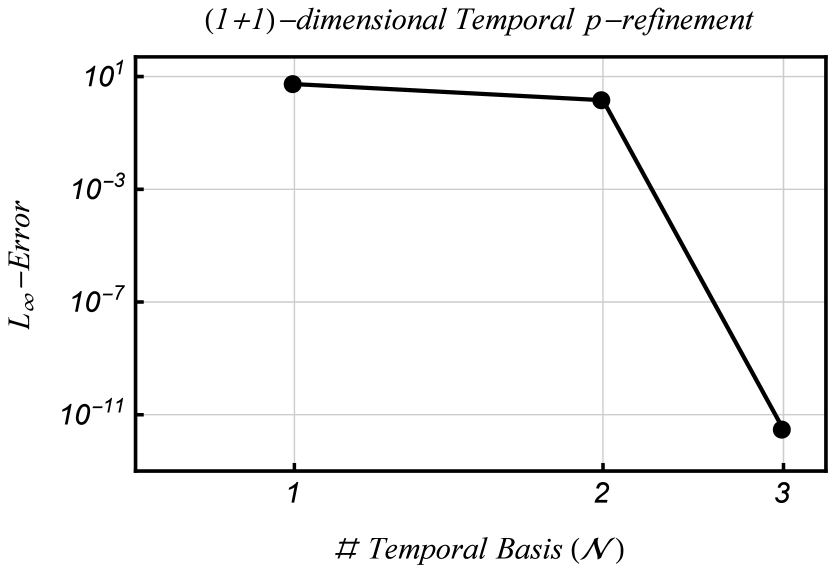
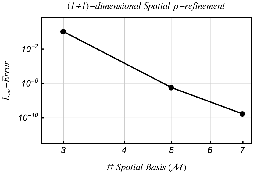
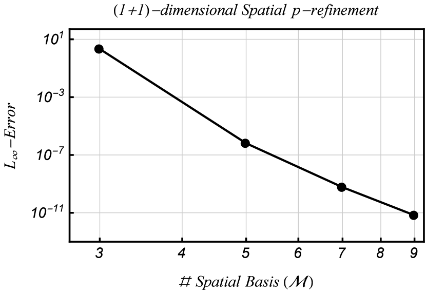
Fig. 1: Temporal/Spatial p-refinement for case I with singularity of order $\alpha=10^{-4}$. (Left): $p_{1}=3$, $p_{2}=p_{3}=2$, and expansion order of $\mathcal{N}\times 9$. (Middle): $p_{1}=2$, $p_{2}=p_{3}=2$, and expansion order of $3\times\mathcal{M}$. (Right): $p_{1}=3$, $p_{2}=p_{3}=2$, and expansion order of $4\times\mathcal{M}$.

Case II: We consider $u^{ext}=t^{p_{1}+\alpha}\sin(2\pi x_{1})$, where $p_{1}=3$, and let $\alpha=0.1$ and $\alpha=0.9$. We set the number of temporal basis functions, $\mathcal{N}=4$, and show the convergence of approximate solution by increasing the number of spatial basis, $\mathcal{M}$ in Fig. 2. The main difficulty in this case is the construction of the load vector. To accurately compute the integrals in the construction of the load vector, we project the spatial part of the forcing function, $\sin(2\pi x_{1})$, on the spatial bases. To make sure that the corresponding error is of machine-precision order and thus, not dominant, we truncate the projection at 25 terms, where there error is of order $10^{-16}$. Therefore, the quadrature rule over derivative order should be performed for 25 terms rather than only a single $\sin(2\pi x_{1})$ term. This will increase the computational cost.

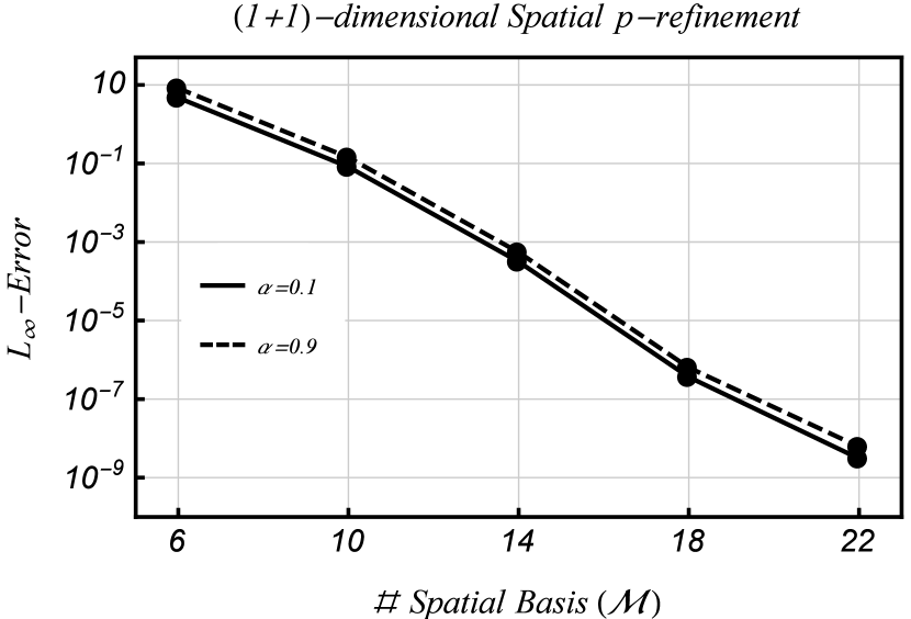
Fig. 2: Spatial p-refinement for case II, $p_{1}=3$, $\alpha=0.1$, and $\alpha=0.9$.

Case III: (High-dimensional p-refinement) We consider the exact solution of the form

(6.2) $$u^{ext}=t^{p_{1}+\alpha}\times\prod_{i=1}^{3}(1+x_{i})^{p_{2i}}(1-x_{i})^{p_{2i+1}}$$

with singularity of order $\alpha=10^{-4}$, where $p_{1}=3$, and $p_{2i}=p_{2i+1}=1$. Similar to previous cases, we set the number of temporal bases, $\mathcal{N}=4$, and study convergence by uniformly increasing the number of spatial bases in all dimensions. Fig. 3 shows the results for $(1+2)$-dimensional and $(1+3)$-dimensional problems with expansion order of $\mathcal{N}\times\mathcal{M}_{1}\times\mathcal{M}_{2}$, and $\mathcal{N}\times\mathcal{M}_{1}\times\mathcal{M}_{2}\times\mathcal{M}_{3}$, respectively. Following Case I, the computed rate of convergence $\bar{r}_{1}=\bar{r}_{2}=\bar{r}_{3}=16.13$ in (6.2) for $\alpha=10^{-4}$ is greater than the minimum regularity of the exact solution $r\approx 2.05$, which is in agreement with Theorem 5.7.

Fig. 3: Spatial p-refinement for case III with singularity of order $\alpha=10^{-4}$. (Left): $(1+2)$-dimensional, $p_{1}=3$, $p_{2i}=p_{2i+1}=1$, where the expansion order is $\mathcal{N}\times\mathcal{M}_{1}\times\mathcal{M}_{2}$. (Left): $(1+3)$-dimensional, $p_{1}=3$, $p_{2i}=p_{2i+1}=1$, where the expansion order is $\mathcal{N}\times\mathcal{M}_{1}\times\mathcal{M}_{2}\times\mathcal{M}_{3}$.

In addition to the convergence study, we examine the efficiency of the developed method and fast solver by comparing the CPU times for $(1+1)$-, $(1+2)$-, and $(1+3)$-dimensional space-time hypercube domains in case III. The computed CPU times are obtained on an INTEL(XEON E52670) processor of 2.5 GHZ, and reported in Table 1.

Table 1: CPU time, PG spectral method for fully distributed (1+d)-dimensional diffusion problems. $u^{ext}=t^{p_{1}+\alpha}\times\prod_{i=1}^{3}(1+x_{i})^{p_{2i}}(1-x_{i})^{p_{2i+1}}$, where $\alpha=10^{-4}$, $p_{1}=3$, and the expansion order is $4\times 11^{d}$.

	$p_{2i}=p_{2i+1}=2$			$p_{2i}=p_{2i+1}=3$
	d=1	d=2	d=3	d=1	d=2	d=3
CPU Time $[$Sec$]$	$1546.81$	$1735.03$	$2358.67$	$1596.16$	$1786.61$	$2407.22$
$\|e\|_{L^{\infty}(\Omega)}$	$6.84\times 10^{-12}$	$4.45\times 10^{-12}$	$3.27\times 10^{-12}$	$6.27\times 10^{-12}$	$3.86\times 10^{-12}$	$2.71\times 10^{-12}$

7 Summary

We developed a unified Petrov-Galerkin spectral method for fully distributed-order PDEs with constant coefficients on a ($1+d$)-dimensional space-time hypercube, subject to homogeneous Dirichlet initial/boundary conditions. We obtained the weak formulation of the problem, and proved the well-posedness by defining the proper underlying distributed Sobolev spaces and the associated norms. We then formulated the numerical scheme, exploiting Jacobi poly-fractonomials as temporal basis/test functions, and Legendre polynomials as spatial basis/test functions. In order to improve efficiency of the proposed method in higher-dimensions, we constructed a unified fast linear solver employing certain properties of the stiffness/mass matrices, which significantly reduced the computation time. Moreover, we proved stability of the developed scheme and carried out the error analysis. Finally, via several numerical test cases, we examined the practical performance of proposed method and illustrated the spectral accuracy.

Appendix: Entries of Spatial Stiffness Matrix

Here, we provide the computation of entries of the spatial stiffness matrix by performing an affine mapping $\vartheta$ from the standard domain $\mu^{stn}_{j}\in[-1,1]$ to $\mu_{j}\in[\mu_{j}^{max},\mu_{j}^{min}]$.

Lemma 7.1.

The total spatial stiffness matrix $S^{Tot}_{j}$ is symmetric and its entries can be exactly computed as:

(7.1) $$S^{\,{Tot}}_{j}=c_{l_{j}}\times S_{l}^{\varrho_{j}}+c_{r_{j}}\times S_{r}^{\varrho_{j}}-\kappa_{l_{j}}\times S_{l}^{\rho_{j}}-\kappa_{r_{j}}\times S_{r}^{\rho_{j}},$$

where $j=1,2,\cdots,d$.

Proof.

Regarding the definition of stiffness matrix, we have

$$\{S_{l}^{\varrho_{j}}\}_{r,n} =\int_{-1}^{1}\int_{\mu_{j}^{min}}^{\mu_{j}^{max}}\varrho_{j}(\mu_{j})\prescript{}{-1}{\mathcal{D}}_{\xi_{j}}^{\mu_{j}}\Big{(}\,\phi_{n}(x_{j})\Big{)}\prescript{}{\xi_{j}}{\mathcal{D}}_{1}^{\mu_{j}}\Big{(}\Phi_{r}(x_{j})\Big{)}\,d{x_{j}},$$

$$=\beta_{1}\int_{-1}^{1}\int_{-1}^{1}\varrho_{j}\big{(}\vartheta(\mu_{j}^{stn})\big{)}\prescript{}{-1}{\mathcal{D}}_{\xi_{j}}^{\mu_{j}^{stn}}\Big{(}\,P_{n+1}({\xi_{j}})-P_{n-1}({\xi_{j}})\Big{)}$$

$$\qquad\qquad\quad\times\prescript{}{{\xi}_{j}}{\mathcal{D}}_{1}^{\mu_{j}^{stn}}\Big{(}\,P_{k+1}({\xi_{j}})-P_{k-1}({\xi_{j}})\Big{)}\,d{\xi_{j}},$$

(7.2) $$=\beta_{1}\Big{[}\,\widetilde{S}^{\,\varrho_{j}}_{r+1,n+1}-\widetilde{S}_{r+1,n-1}^{\,\varrho_{j}}-\widetilde{S}_{r-1,n+1}^{\,\varrho_{j}}+\widetilde{S}_{r-1,n-1}^{\,\varrho_{j}}\Big{]},\quad\quad$$

where $\beta_{1}={\widetilde{\sigma}}_{r}\,\sigma_{n}\,\Big{(}\frac{\mu_{j}^{max}-\mu_{j}^{min}}{2}\Big{)}$ and

$$\widetilde{S}_{r,n}^{\varrho_{j}} =\,\int_{-1}^{1}\int_{-1}^{1}\varrho_{j}\big{(}\vartheta(\mu_{j}^{stn})\big{)}\prescript{}{-1}{\mathcal{D}}_{\xi_{j}}^{\mu_{j}^{stn}}\Big{(}\,P_{n}(\xi_{j})\Big{)}\prescript{}{\xi_{j}}{\mathcal{D}}_{1}^{\mu_{j}^{stn}}\Big{(}\,P_{r}(\xi_{j})\Big{)}\,d{\xi_{j}}\,d\mu_{j}^{stn}$$

$$=\int_{-1}^{1}\varrho_{j}\big{(}\vartheta(\mu_{j}^{stn})\big{)}\,\frac{\Gamma(r+1)}{\Gamma(r-\mu_{j}^{stn}+1)}\,\frac{\Gamma(n+1)}{\Gamma(n-\mu_{j}^{stn}+1)}\,$$

$$\,\times\int_{-1}^{1}{(1-\xi_{j}^{2})}^{-\mu_{j}^{stn}}\,P^{-\mu_{j}^{stn},\mu_{j}^{stn}}_{r}\,P^{\mu_{j}^{stn},-\mu_{j}^{stn}}_{n}d{\xi_{j}}\,d\mu_{j}^{stn}.$$

$\widetilde{S}_{r,n}^{\varrho_{j}}$ can be computed accurately using Gauss-Legendre (GL) quadrature rules as

(7.3) $$\widetilde{S}_{r,n}^{\varrho_{j}^{stn}} = \sum_{q=1}^{Q}\frac{\Gamma(r+1)}{\Gamma(r-\mu_{j}^{stn}|_{q}+1)}\frac{\Gamma(n+1)}{\Gamma(n-\mu_{j}^{stn}|_{q}+1)}\varrho_{j}|_{q}\,w_{q}\,\times$$

$$\int_{-1}^{1}{(1-\xi_{j}^{2})}^{-\mu_{j}^{stn}|_{q}}\,P^{-\mu_{j}^{stn}|_{q},\mu_{j}^{stn}|_{q}}_{r}(\xi_{j})\,P^{\mu_{j}^{stn}|_{q},-\mu_{j}^{stn}|_{q}}_{n}(\xi_{j})d{\xi_{j}},\quad$$

in which $\mathcal{Q}\geq\mathcal{M}_{j}+2$ represents the minimum number of GL quadrature points $\{\mu_{j}^{stn}|_{q}\}_{q=1}^{\mathcal{Q}}$ for exact quadrature, and $\{w_{q}\}_{q=1}^{Q}$ are the corresponding quadrature weights. Exploiting the property of the Jacobi polynomials where $P^{\alpha,\beta}_{n}(-\xi_{j})=(-1)^{n}P^{\beta,\alpha}_{n}(\xi_{j})$, we have $\widetilde{S}_{r,n}^{\,\varrho_{j}^{stn}}=(-1)^{(r+n)}\,\widetilde{S}_{n,r}^{\,\varrho_{j}^{stn}}$. Following [48], ${\widetilde{\sigma}}_{r}$ and $\sigma_{n}$ are chosen such that $(-1)^{(n+r)}$ is canceled. Accordingly, $\{S_{l}^{\varrho_{j}}\}_{n,r}=\{S_{l}^{\varrho_{j}}\}_{r,n}=\{S_{r}^{\varrho_{j}}\}_{r,n}=\{S_{r}^{\varrho_{j}}\}_{r,n}$ due to the symmetry of $S_{l}^{\varrho_{j}}$ and $S_{r}^{\varrho_{j}}$. Similarly, we get $\{S_{l}^{\rho_{j}}\}_{n,r}=\{S_{l}^{\rho_{j}}\}_{r,n}=\{S_{r}^{\rho_{j}}\}_{n,r}=\{S_{r}^{\rho_{j}}\}_{r,n}$. Eventually, we conclude that the stiffness matrix $S^{\,\varrho_{j}}_{l}$, $S^{\,\varrho_{j}}_{r}$, $S^{\,\rho_{j}}_{l}$, $S^{\,\rho_{j}}_{r}$, and thereby $\{S^{Tot}_{j}\}_{n,r}$ as the sum of symmetric matrices are symmetric. ∎

References

- [1] Mostafa Abbaszadeh and Mehdi Dehghan, An improved meshless method for solving two-dimensional distributed order time-fractional diffusion-wave equation with error estimate, Numerical Algorithms, 75 (2017), pp. 173–211.
- [2] Mark Ainsworth and Christian Glusa, Aspects of an adaptive finite element method for the fractional laplacian: a priori and a posteriori error estimates, efficient implementation and multigrid solver, Computer Methods in Applied Mechanics and Engineering, 327 (2017), pp. 4–35.
- [3] Moulay Rchid Sidi Ammi and Ismail Jamiai, Finite difference and legendre spectral method for a time-fractinal diffusion-convection equation for image restoration, Discrete & Continuous Dynamical Systems-Series S, 11 (2018).
- [4] Abbas Ghasempour Ardakani, Investigation of brewster anomalies in one-dimensional disordered media having lévy-type distribution, The European Physical Journal B, 89 (2016), p. 76.
- [5] Kyle C Armour, John Marshall, Jeffery R Scott, Aaron Donohoe, and Emily R Newsom, Southern ocean warming delayed by circumpolar upwelling and equatorward transport, Nature Geoscience, 9 (2016), pp. 549–554.
- [6] D. A. Benson, S. W. Wheatcraft, and M. M. Meerschaert, Application of a fractional advection-dispersion equation, Water Resources Research, 36 (2000), pp. 1403–1412.
- [7] AV Chechkin, Rudolf Gorenflo, and IM Sokolov, Retarding subdiffusion and accelerating superdiffusion governed by distributed-order fractional diffusion equations, Physical Review E, 66 (2002), p. 046129.
- [8] Sheng Chen, Jie Shen, and Li-Lian Wang, Generalized jacobi functions and their applications to fractional differential equations, Mathematics of Computation, 85 (2016), pp. 1603–1638.
- [9] , Laguerre functions and their applications to tempered fractional differential equations on infinite intervals, Journal of Scientific Computing, (2017), pp. 1–28.
- [10] Aijie Cheng, Hong Wang, and Kaixin Wang, A eulerian–lagrangian control volume method for solute transport with anomalous diffusion, Numerical Methods for Partial Differential Equations, 31 (2015), pp. 253–267.
- [11] A Coronel-Escamilla, JF Gómez-Aguilar, L Torres, and RF Escobar-Jiménez, A numerical solution for a variable-order reaction–diffusion model by using fractional derivatives with non-local and non-singular kernel, Physica A: Statistical Mechanics and its Applications, 491 (2018), pp. 406–424.
- [12] Beiping Duan, Bangti Jin, Raytcho Lazarov, Joseph Pasciak, and Zhi Zhou, Space-time petrov–galerkin fem for fractional diffusion problems, Computational Methods in Applied Mathematics (2017), (2017).
- [13] Jun-Sheng Duan and Dumitru Baleanu, Steady periodic response for a vibration system with distributed order derivatives to periodic excitation, Journal of Vibration and Control, p. 1077546317700989.
- [14] C.H. Eab and S.C. Lim, Fractional langevin equations of distributed order, Physical Review E, 83 (2011), p. 031136.
- [15] Yaniv Edery, Ishai Dror, Harvey Scher, and Brian Berkowitz, Anomalous reactive transport in porous media: Experiments and modeling, Physical Review E, 91 (2015), p. 052130.
- [16] Vincent J Ervin and John Paul Roop, Variational solution of fractional advection dispersion equations on bounded domains in rd, Numerical Methods for Partial Differential Equations, 23 (2007), p. 256.
- [17] Wenping Fan and Fawang Liu, A numerical method for solving the two-dimensional distributed order space-fractional diffusion equation on an irregular convex domain, Applied Mathematics Letters, 77 (2018), pp. 114–121.
- [18] Rudolf Gorenflo, Yuri Luchko, and Masahiro Yamamoto, Time-fractional diffusion equation in the fractional sobolev spaces, Fractional Calculus and Applied Analysis, 18 (2015), pp. 799–820.
- [19] Igor Goychuk, Anomalous transport of subdiffusing cargos by single kinesin motors: the role of mechano–chemical coupling and anharmonicity of tether, Physical biology, 12 (2015), p. 016013.
- [20] Takahiro Iwayama, Shinya Murakami, and Takeshi Watanabe, Anomalous eddy viscosity for two-dimensional turbulence, Physics of Fluids, 27 (2015), p. 045104.
- [21] Bangti Jin, Raytcho Lazarov, Dongwoo Sheen, and Zhi Zhou, Error estimates for approximations of distributed order time fractional diffusion with nonsmooth data, Fractional Calculus and Applied Analysis, 19 (2016), pp. 69–93.
- [22] Bangti Jin, Raytcho Lazarov, Vidar Thomée, and Zhi Zhou, On nonnegativity preservation in finite element methods for subdiffusion equations, Mathematics of Computation, 86 (2017), pp. 2239–2260.
- [23] Ehsan Kharazmi and Mohsen Zayernouri, Fractional pseudo-spectral methods for distributed-order fractional pdes, International Journal of Computer Mathematics, 95 (2018), pp. 1340–1361.
- [24] Ehsan Kharazmi, Mohsen Zayernouri, and George Em Karniadakis, Petrov–galerkin and spectral collocation methods for distributed order differential equations, SIAM Journal on Scientific Computing, 39 (2017), pp. A1003–A1037.
- [25] , A petrov–galerkin spectral element method for fractional elliptic problems, Computer Methods in Applied Mechanics and Engineering, 324 (2017), pp. 512–536.
- [26] R. Klages, G. Radons, and I. M. Sokolov, Anomalous Transport: Foundations and Applications, Wiley-VCH, 2008.
- [27] Sanja Konjik, Ljubica Oparnica, and Dusan Zorica, Distributed order fractional constitutive stress-strain relation in wave propagation modeling, arXiv preprint arXiv:1709.01339, (2017).
- [28] Xiaoli Li and Hongxing Rui, Two temporal second-order h1-galerkin mixed finite element schemes for distributed-order fractional sub-diffusion equations, Numerical Algorithms, (2018), p. (in press).
- [29] Xianjuan Li and Chuanju Xu, A space-time spectral method for the time fractional diffusion equation, SIAM Journal on Numerical Analysis, 47 (2009), pp. 2108–2131.
- [30] , Existence and uniqueness of the weak solution of the space-time fractional diffusion equation and a spectral method approximation, Communications in Computational Physics, 8 (2010), p. 1016.
- [31] Hong-lin Liao, Pin Lyu, Seakweng Vong, and Ying Zhao, Stability of fully discrete schemes with interpolation-type fractional formulas for distributed-order subdiffusion equations, Numerical Algorithms, 75 (2017), pp. 845–878.
- [32] Yury Luchko, Boundary value problems for the generalized time-fractional diffusion equation of distributed order, Fract. Calc. Appl. Anal, 12 (2009), pp. 409–422.
- [33] JE Macías-Díaz, An explicit dissipation-preserving method for riesz space-fractional nonlinear wave equations in multiple dimensions, Communications in Nonlinear Science and Numerical Simulation, 59 (2018), pp. 67–87.
- [34] Y Maday, Analysis of spectral projectors in one-dimensional domains, mathematics of computation, 55 (1990), pp. 537–562.
- [35] Francesco Mainardi, Antonio Mura, Rudolf Gorenflo, and Mirjana Stojanović, The two forms of fractional relaxation of distributed order, Journal of Vibration and Control, 13 (2007), pp. 1249–1268.
- [36] Francesco Mainardi, Antonio Mura, Gianni Pagnini, and Rudolf Gorenflo, Time-fractional diffusion of distributed order, Journal of Vibration and Control, 14 (2008), pp. 1267–1290.
- [37] Zhiping Mao and Jie Shen, Efficient spectral–galerkin methods for fractional partial differential equations with variable coefficients, Journal of Computational Physics, 307 (2016), pp. 243–261.
- [38] , Spectral element method with geometric mesh for two-sided fractional differential equations, Advances in Computational Mathematics, (2017), pp. 1–27.
- [39] RA Mashelkar and G Marrucci, Anomalous transport phenomena in rapid external flows of viscoelastic fluids, Rheologica Acta, 19 (1980), pp. 426–431.
- [40] Mark M Meerschaert, Fractional calculus, anomalous diffusion, and probability, in Fractional Dynamics: Recent Advances, World Scientific, 2012, pp. 265–284.
- [41] Mark M Meerschaert and Alla Sikorskii, Stochastic models for fractional calculus, vol. 43, Walter de Gruyter, 2012.
- [42] Ralf Metzler, Jae-Hyung Jeon, Andrey G Cherstvy, and Eli Barkai, Anomalous diffusion models and their properties: non-stationarity, non-ergodicity, and ageing at the centenary of single particle tracking, Physical Chemistry Chemical Physics, 16 (2014), pp. 24128–24164.
- [43] Ralf Metzler and Joseph Klafter, The random walk’s guide to anomalous diffusion: a fractional dynamics approach, Physics reports, 339 (2000), pp. 1–77.
- [44] M. Naghibolhosseini, Estimation of outer-middle ear transmission using DPOAEs and fractional-order modeling of human middle ear, PhD thesis, City University of New York, NY., 2015.
- [45] Maryam Naghibolhosseini and Glenis R Long, Fractional-order modelling and simulation of human ear, International Journal of Computer Mathematics, (2017), pp. 1–17.
- [46] Paris Perdikaris and George Em Karniadakis, Fractional-order viscoelasticity in one-dimensional blood flow models, Annals of biomedical engineering, 42 (2014), pp. 1012–1023.
- [47] Benjamin Michael Regner, Randomness in biological transport, (2014).
- [48] Mehdi Samiee, Mohsen Zayernouri, and Mark M. Meerschaert, A unified spectral method for fpdes with two-sided derivatives; part i: A fast solver, Journal of Computational Physics, 2018 (in press), (2018).
- [49] Mehdi Samiee, Mohsen Zayernouri, and Mark M Meerschaert, A unified spectral method for fpdes with two-sided derivatives; stability, and error analysis, Journal of Computational Physics, 2018 (in press), (2018).
- [50] Jie Shen, Tao Tang, and Li-Lian Wang, Spectral methods: algorithms, analysis and applications, vol. 41, Springer Science & Business Media, 2011.
- [51] Boris I Shraiman and Eric D Siggia, Scalar turbulence, Nature, 405 (2000), pp. 639–646.
- [52] IM Sokolov, AV Chechkin, and J Klafter, Distributed-order fractional kinetics, arXiv preprint cond-mat/0401146, (2004).
- [53] JL Suzuki, M Zayernouri, ML Bittencourt, and GE Karniadakis, Fractional-order uniaxial visco-elasto-plastic models for structural analysis, Computer Methods in Applied Mechanics and Engineering, 308 (2016), pp. 443–467.
- [54] WenYi Tian, Han Zhou, and Weihua Deng, A class of second order difference approximations for solving space fractional diffusion equations, Mathematics of Computation, 84 (2015), pp. 1703–1727.
- [55] Živorad Tomovski and Trifce Sandev, Distributed-order wave equations with composite time fractional derivative, International Journal of Computer Mathematics, (2017), pp. 1–14.
- [56] Alina Tyukhova, Marco Dentz, Wolfgang Kinzelbach, and Matthias Willmann, Mechanisms of anomalous dispersion in flow through heterogeneous porous media, Physical Review Fluids, 1 (2016), p. 074002.
- [57] Masahiro Yamamoto, Weak solutions to non-homogeneous boundary value problems for time-fractional diffusion equations, Journal of Mathematical Analysis and Applications, 460 (2018), pp. 365–381.
- [58] Mahmoud A Zaky, A legendre collocation method for distributed-order fractional optimal control problems, Nonlinear Dynamics, (2018), pp. 1–15.
- [59] Mohsen Zayernouri, Mark Ainsworth, and George Em Karniadakis, Tempered fractional sturm–liouville eigenproblems, SIAM Journal on Scientific Computing, 37 (2015), pp. A1777–A1800.
- [60] , A unified petrov–galerkin spectral method for fractional pdes, Computer Methods in Applied Mechanics and Engineering, 283 (2015), pp. 1545–1569.
- [61] Mohsen Zayernouri and George Em Karniadakis, Fractional sturm–liouville eigen-problems: theory and numerical approximation, Journal of Computational Physics, 252 (2013), pp. 495–517.
- [62] Yong Zhang, Mark M Meerschaert, Boris Baeumer, and Eric M LaBolle, Modeling mixed retention and early arrivals in multidimensional heterogeneous media using an explicit lagrangian scheme, Water Resources Research, 51 (2015), pp. 6311–6337.
- [63] Yong Zhang, Mark M Meerschaert, and Roseanna M Neupauer, Backward fractional advection dispersion model for contaminant source prediction, Water Resources Research, 52 (2016), pp. 2462–2473.