Sparse and Constrained Attention for Neural Machine Translation

Abstract

In NMT, words are sometimes dropped from the source or generated repeatedly in the translation. We explore novel strategies to address the coverage problem that change only the attention transformation. Our approach allocates fertilities to source words, used to bound the attention each word can receive. We experiment with various sparse and constrained attention transformations and propose a new one, constrained sparsemax, shown to be differentiable and sparse. Empirical evaluation is provided in three languages pairs.

1 Introduction

Neural machine translation (NMT) emerged in the last few years as a very successful paradigm (Sutskever et al., 2014; Bahdanau et al., 2014; Gehring et al., 2017; Vaswani et al., 2017). While NMT is generally more fluent than previous statistical systems, adequacy is still a major concern Koehn and Knowles (2017): common mistakes include dropping source words and repeating words in the generated translation.

Previous work has attempted to mitigate this problem in various ways. Wu et al. (2016) incorporate coverage and length penalties during beam search—a simple yet limited solution, since it only affects the scores of translation hypotheses that are already in the beam. Other approaches involve architectural changes: providing coverage vectors to track the attention history Mi et al. (2016); Tu et al. (2016), using gating architectures and adaptive attention to control the amount of source context provided Tu et al. (2017a); Li and Zhu (2017), or adding a reconstruction loss Tu et al. (2017b). Feng et al. (2016) also use the notion of fertility implicitly in their proposed model. Their “fertility conditioned decoder” uses a coverage vector and an “extract gate” which are incorporated in the decoding recurrent unit, increasing the number of parameters.

In this paper, we propose a different solution that does not change the overall architecture, but only the attention transformation. Namely, we replace the traditional softmax by other recently proposed transformations that either promote attention sparsity (Martins and Astudillo, 2016) or upper bound the amount of attention a word can receive (Martins and Kreutzer, 2017). The bounds are determined by the fertility values of the source words. While these transformations have given encouraging results in various NLP problems, they have never been applied to NMT, to the best of our knowledge. Furthermore, we combine these two ideas and propose a novel attention transformation, constrained sparsemax, which produces both sparse and bounded attention weights, yielding a compact and interpretable set of alignments. While being in-between soft and hard alignments (Figure 2), the constrained sparsemax transformation is end-to-end differentiable, hence amenable for training with gradient backpropagation.

To sum up, our contributions are as follows:

• We formulate constrained sparsemax and derive efficient linear and sublinear-time algorithms for running forward and backward propagation. This transformation has two levels of sparsity: over time steps, and over the attended words at each step.

• We provide a detailed empirical comparison of various attention transformations, including softmax (Bahdanau et al., 2014), sparsemax (Martins and Astudillo, 2016), constrained softmax (Martins and Kreutzer, 2017), and our newly proposed constrained sparsemax. We provide error analysis including two new metrics targeted at detecting coverage problems.

2 Preliminaries

Our underlying model architecture is a standard attentional encoder-decoder (Bahdanau et al., 2014). Let $x:=x_{1:J}$ and $y:=y_{1:T}$ denote the source and target sentences, respectively. We use a Bi-LSTM encoder to represent the source words as a matrix $\bm{H}:=[\bm{h}_{1},\ldots,\bm{h}_{J}]\in\mathbb{R}^{2D\times J}$. The conditional probability of the target sentence is given as

$$\textstyle p(y\,\,|\,\,x):=\prod_{t=1}^{T}p(y_{t}\,\,|\,\,y_{1:(t-1)},x),$$ (1)

where $p(y_{t}\,\,|\,\,y_{1:(t-1)},x)$ is computed by a softmax output layer that receives a decoder state $\bm{s}_{t}$ as input. This state is updated by an auto-regressive LSTM, $\bm{s}_{t}=\operatorname*{\mathsf{RNN}}(\operatorname*{\mathsf{embed}}(y_{t-1}),\bm{s}_{t-1},\bm{c}_{t})$, where $\bm{c}_{t}$ is an input context vector. This vector is computed as $\bm{c}_{t}:=\bm{H}\bm{\alpha}_{t}$, where $\bm{\alpha}_{t}$ is a probability distribution that represents the attention over the source words, commonly obtained as

$$\bm{\alpha}_{t}=\operatorname*{\mathsf{softmax}}(\bm{z}_{t}),$$ (2)

where $\bm{z}_{t}\in\mathbb{R}^{J}$ is a vector of scores. We follow Luong et al. (2015) and define $z_{t,j}:=\bm{s}_{t-1}^{\top}\bm{W}\bm{h}_{j}$ as a bilinear transformation of encoder and decoder states, where $\bm{W}$ is a model parameter.

3 Sparse and Constrained Attention

In this work, we consider alternatives to Eq. 2. Since the softmax is strictly positive, it forces all words in the source to receive some probability mass in the resulting attention distribution, which can be wasteful. Moreover, it may happen that the decoder attends repeatedly to the same source words across time steps, causing repetitions in the generated translation, as Tu et al. (2016) observed.

With this in mind, we replace Eq. 2 by $\bm{\alpha}_{t}=\rho(\bm{z}_{t},\bm{u}_{t})$, where $\rho$ is a transformation that may depend both on the scores $\bm{z}_{t}\in\mathbb{R}^{J}$ and on upper bounds $\bm{u}_{t}\in\mathbb{R}^{J}$ that limit the amount of attention that each word can receive. We consider three alternatives to softmax, described next.

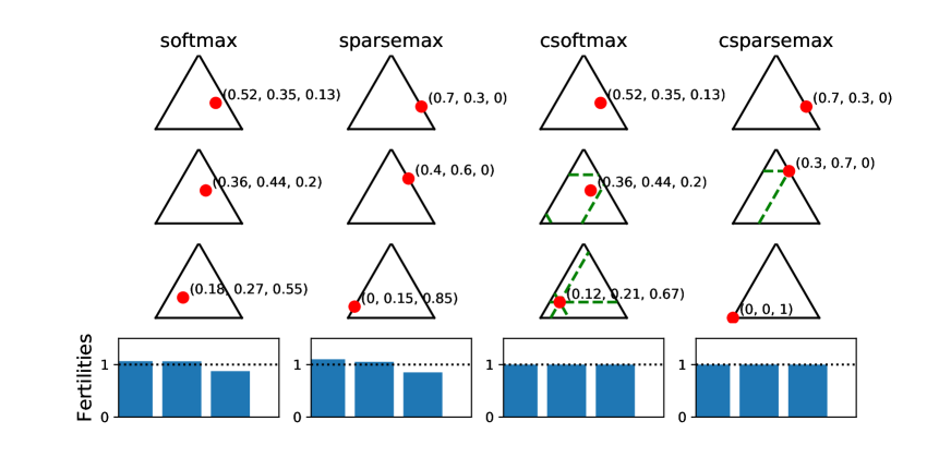
Figure 1: Illustration of the different attention transformations for a toy example with three source words. We show the attention values on the probability simplex. In the first row we assume scores $\bm{z}=(1.2,0.8,-0.2)$, and in the second and third rows $\bm{z}=(0.7,0.9,0.1)$ and $\bm{z}=(-0.2,0.2,0.9)$, respectively. For constrained softmax/sparsemax, we set unit fertilities to every word; for each row the upper bounds (represented as green dashed lines) are set as the difference between these fertilities and the cumulative attention each word has received. The last row illustrates the cumulative attention for the three words after all rounds.

Sparsemax.

The sparsemax transformation (Martins and Astudillo, 2016) is defined as:

$$\operatorname*{\mathsf{sparsemax}}(\bm{z}) := \operatorname*{\mathsf{arg\,min}}_{\bm{\alpha}\in\Delta^{J}}\|\bm{\alpha}-\bm{z}\|^{2},$$ (3)

where $\Delta^{J}:=\{\bm{\alpha}\in\mathbb{R}^{J}\,\,|\,\,\ \bm{\alpha}\geq\mathbf{0},\sum_{j}\alpha_{j}=1\}$. In words, it is the Euclidean projection of the scores $\bm{z}$ onto the probability simplex. These projections tend to hit the boundary of the simplex, yielding a sparse probability distribution. This allows the decoder to attend only to a few words in the source, assigning zero probability mass to all other words. Martins and Astudillo (2016) have shown that the sparsemax can be evaluated in $O(J)$ time (same asymptotic cost as softmax) and gradient backpropagation takes sublinear time (faster than softmax), by exploiting the sparsity of the solution.

Constrained softmax.

The constrained softmax transformation was recently proposed by Martins and Kreutzer (2017) in the context of easy-first sequence tagging, being defined as follows:

$$\operatorname*{\mathsf{csoftmax}}(\bm{z};\bm{u}) \!\!:=\!\! \operatorname*{\mathsf{arg\,min}}_{\bm{\alpha}\in\Delta^{J}}\mathsf{KL}(\bm{\alpha}\|\operatorname*{\mathsf{softmax}}(\bm{z}))$$ (4)

$$\qquad\text{s.t.}\quad\bm{\alpha}\leq\bm{u},$$

where $\bm{u}$ is a vector of upper bounds, and $\mathsf{KL}(.\|.)$ is the Kullback-Leibler divergence. In other words, it returns the distribution closest to $\operatorname*{\mathsf{softmax}}(\bm{z})$ whose attention probabilities are bounded by $\bm{u}$. Martins and Kreutzer (2017) have shown that this transformation can be evaluated in $O(J\log J)$ time and its gradients backpropagated in $O(J)$ time.

To use this transformation in the attention mechanism, we make use of the idea of fertility (Brown et al., 1993). Namely, let $\bm{\beta}_{t-1}:=\sum_{\tau=1}^{t-1}\bm{\alpha}_{\tau}$ denote the cumulative attention that each source word has received up to time step $t$, and let $\bm{f}:=(f_{j})_{j=1}^{J}$ be a vector containing fertility upper bounds for each source word. The attention at step $t$ is computed as

$$\bm{\alpha}_{t}=\operatorname*{\mathsf{csoftmax}}(\bm{z}_{t},\bm{f}-\bm{\beta}_{t-1}).$$ (5)

Intuitively, each source word $j$ gets a credit of $f_{j}$ units of attention, which are consumed along the decoding process. If all the credit is exhausted, it receives zero attention from then on. Unlike the sparsemax transformation, which places sparse attention over the source words, the constrained softmax leads to sparsity over time steps.

Constrained sparsemax.

In this work, we propose a novel transformation which shares the two properties above: it provides both sparse and bounded probabilities. It is defined as:

$$\operatorname*{\mathsf{csparsemax}}(\bm{z};\bm{u}) \!\!:=\!\! \operatorname*{\mathsf{arg\,min}}_{\bm{\alpha}\in\Delta^{J}}\|\bm{\alpha}-\bm{z}\|^{2}$$ (6)

$$\qquad\text{s.t.}\quad\bm{\alpha}\leq\bm{u}.$$

The following result, whose detailed proof we include as supplementary material (Appendix A), is key for enabling the use of the constrained sparsemax transformation in neural networks.

Proposition 1

Let $\bm{\alpha}^{\star}=\operatorname*{\mathsf{csparsemax}}(\bm{z};\bm{u})$ be the solution of Eq. 6, and define the sets $\mathcal{A}=\{j\in[J]\,\,|\,\,0<\alpha_{j}^{\star}<u_{j}\}$, $\mathcal{A}_{L}=\{j\in[J]\,\,|\,\,\alpha_{j}^{\star}=0\}$, and $\mathcal{A}_{R}=\{j\in[J]\,\,|\,\,\alpha_{j}^{\star}=u_{j}\}$. Then:

• Forward propagation. $\bm{\alpha}^{\star}$ can be computed in $O(J)$ time with the algorithm of Pardalos and Kovoor (1990) (Alg. 1 in Appendix A). The solution takes the form $\alpha_{j}^{\star}=\max\{0,\min\{u_{j},z_{j}-\tau\}\}$, where $\tau$ is a normalization constant.

• Gradient backpropagation. Backpropagation takes sublinear time $O(|\mathcal{A}|+|\mathcal{A_{R}}|)$. Let $L(\bm{\theta})$ be a loss function, $\mathrm{d}\bm{\alpha}=\nabla_{\bm{\alpha}}L(\bm{\theta})$ be the output gradient, and $\mathrm{d}\bm{z}=\nabla_{\bm{z}}L(\bm{\theta})$ and $\mathrm{d}\bm{u}=\nabla_{\bm{u}}L(\bm{\theta})$ be the input gradients. Then, we have:

  $$\mathrm{d}z_{j} = \mathds{1}(j\in\mathcal{A})(\mathrm{d}\alpha_{j}-m)$$ (7)

  $$\mathrm{d}u_{j} = \mathds{1}(j\in\mathcal{A}_{R})(\mathrm{d}\alpha_{j}-m),$$ (8)

  where $m=\frac{1}{|\mathcal{A}|}\sum_{j\in\mathcal{A}}\mathrm{d}\alpha_{j}$.

4 Fertility Bounds

We experiment with three ways of setting the fertility of the source words: constant, guided, and predicted. With constant, we set the fertilities of all source words to a fixed integer value $f$. With guided, we train a word aligner based on IBM Model 2 (we used fast_align in our experiments, Dyer et al. (2013)) and, for each word in the vocabulary, we set the fertilities to the maximal observed value in the training data (or 1 if no alignment was observed). With the predicted strategy, we train a separate fertility predictor model using a bi-LSTM tagger. At training time, we provide as supervision the fertility estimated by fast_align. Since our model works with fertility upper bounds and the word aligner may miss some word pairs, we found it beneficial to add a constant to this number (1 in our experiments). At test time, we use the expected fertilities according to our model.

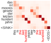
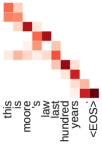
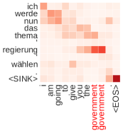
Figure 2: Attention maps for $\operatorname*{\mathsf{softmax}}$ and $\operatorname*{\mathsf{csparsemax}}$ for two De-En sentence pairs (white means zero attention). Repeated words are highlighted. The reference translations are “This is Moore’s law over the last hundred years” and “I am going to go ahead and select government.”

	De-En				Ja-En				Ro-En
	bleu	meteor	rep	drop	bleu	meteor	rep	drop	bleu	meteor	rep	drop
$\operatorname*{\mathsf{softmax}}$	29.51	31.43	3.37	5.89	20.36	23.83	13.48	23.30	29.67	32.05	2.45	5.59
$\operatorname*{\mathsf{softmax}}$ + CovPenalty	29.69	31.53	3.47	5.74	20.70	24.12	14.12	22.79	29.81	32.15	2.48	5.49
$\operatorname*{\mathsf{softmax}}$ + CovVector	29.63	31.54	2.93	5.65	21.53	24.50	11.07	22.18	30.08	32.22	2.42	5.47
$\operatorname*{\mathsf{sparsemax}}$	29.73	31.54	3.18	5.90	21.28	24.25	13.09	22.40	29.97	32.12	2.19	5.60
$\operatorname*{\mathsf{sparsemax}}$ + CovPenalty	29.83	31.60	3.24	5.79	21.64	24.49	13.36	21.91	30.07	32.20	2.20	5.47
$\operatorname*{\mathsf{sparsemax}}$ + CovVector	29.22	31.18	3.13	6.15	21.35	24.74	10.11	21.25	29.30	31.84	2.18	5.87
$\operatorname*{\mathsf{csoftmax}}$ ($c=0.2$)	29.39	31.33	3.29	5.86	20.71	24.00	12.38	22.73	29.39	31.83	2.37	5.64
$\operatorname*{\mathsf{csparsemax}}$ ($c=0.2$)	29.85	31.76	2.67	5.23	21.31	24.51	11.40	21.59	29.77	32.10	1.98	5.44

Table 1: BLEU, METEOR, REP and DROP scores on the test sets for different attention transformations.

	bleu	meteor
constant, $f=2$	29.66	31.60
constant, $f=3$	29.64	31.56
guided,	29.56	31.45
predicted, $c=0$	29.78	31.60
predicted, $c=0.2$	29.85	31.76

Table 2: Impact of various fertility strategies for the $\operatorname*{\mathsf{csparsemax}}$ attention model (De-En).

Sink token.

We append an additional $<$sink$>$ token to the end of the source sentence, to which we assign unbounded fertility ($f_{J+1}=\infty$). The token is akin to the null alignment in IBM models. The reason we add this token is the following: without the sink token, the length of the generated target sentence can never exceed $\sum_{j}f_{j}$ words if we use constrained softmax/sparsemax. At training time this may be problematic, since the target length is fixed and the problems in Eqs. 4–6 can become infeasible. By adding the sink token we guarantee $\sum_{j}f_{j}=\infty$, eliminating the problem.

Exhaustion strategies.

To avoid missing source words, we implemented a simple strategy to encourage more attention to words with larger credit: we redefine the pre-attention word scores as $\bm{z}_{t}^{\prime}=\bm{z}_{t}+c\bm{u}_{t}$, where $c$ is a constant ($c=0.2$ in our experiments). This increases the score of words which have not yet exhausted their fertility (we may regard it as a “soft” lower bound in Eqs. 4–6).

5 Experiments

We evaluated our attention transformations on three language pairs. We focused on small datasets, as they are the most affected by coverage mistakes. We use the IWSLT 2014 corpus for De-En, the KFTT corpus for Ja-En (Neubig, 2011), and the WMT 2016 dataset for Ro-En. The training sets have 153,326, 329,882, and 560,767 parallel sentences, respectively. Our reason to prefer smaller datasets is that this regime is what brings more adequacy issues and demands more structural biases, hence it is a good test bed for our methods. We tokenized the data using the Moses scripts and preprocessed it with subword units Sennrich et al. (2016) with a joint vocabulary and 32k merge operations. Our implementation was done on a fork of the OpenNMT-py toolkit Klein et al. (2017) with the default parameters . We used a validation set to tune hyperparameters introduced by our model. Even though our attention implementations are CPU-based using NumPy (unlike the rest of the computation which is done on the GPU), we did not observe any noticeable slowdown using multiple devices.

As baselines, we use softmax attention, as well as two recently proposed coverage models:

• CovPenalty (Wu et al., 2016, §7). At test time, the hypotheses in the beam are rescored with a global score that includes a length and a coverage penalty. We tuned $\alpha$ and $\beta$ with grid search on $\{0.2k\}_{k=0}^{5}$, as in Wu et al. (2016).

• CovVector (Tu et al., 2016). At training and test time, coverage vectors $\bm{\beta}$ and additional parameters $\bm{v}$ are used to condition the next attention step. We adapted this to our bilinear attention by defining $z_{t,j}=\bm{s}_{t-1}^{\top}(\bm{W}\bm{h}_{j}+\bm{v}{\beta}_{t-1,j})$.

We also experimented combining the strategies above with the sparsemax transformation.

As evaluation metrics, we report tokenized BLEU, METEOR (Denkowski and Lavie (2014), as well as two new metrics that we describe next to account for over and under-translation.

REP-score:

a new metric to count repetitions. Formally, given an $n$-gram $s\in V^{n}$, let $t(s)$ and $r(s)$ be the its frequency in the model translation and reference. We first compute a sentence-level score

$$\sigma(t,r) = \textstyle\lambda_{1}\sum_{s\in V^{n},\,\,t(s)\geq 2}\max\{0,t(s)-r(s)\}$$

$$+ \textstyle\lambda_{2}\sum_{w\in V}\max\{0,t(ww)-r(ww)\}.$$

The REP-score is then given by summing $\sigma(t,r)$ over sentences, normalizing by the number of words on the reference corpus, and multiplying by 100. We used $n=2$, $\lambda_{1}=1$ and $\lambda_{2}=2$.

DROP-score:

a new metric that accounts for possibly dropped words. To compute it, we first compute two sets of word alignments: from source to reference translation, and from source to the predicted translation. In our experiments, the alignments were obtained with fast_align Dyer et al. (2013), trained on the training partition of the data. Then, the DROP-score computes the percentage of source words that aligned with some word from the reference translation, but not with any word from the predicted translation.

Table 1 shows the results. We can see that on average, the sparse models ($\operatorname*{\mathsf{csparsemax}}$ as well as $\operatorname*{\mathsf{sparsemax}}$ combined with coverage models) have higher scores on both BLEU and METEOR. Generally, they also obtain better REP and DROP scores than $\operatorname*{\mathsf{csoftmax}}$ and $\operatorname*{\mathsf{softmax}}$, which suggests that sparse attention alleviates the problem of coverage to some extent.

To compare different fertility strategies, we ran experiments on the De-En for the $\operatorname*{\mathsf{csparsemax}}$ transformation (Table 2). We see that the Predicted strategy outperforms the others both in terms of BLEU and METEOR, albeit slightly.

Figure 2 shows examples of sentences for which the $\operatorname*{\mathsf{csparsemax}}$ fixed repetitions, along with the corresponding attention maps. We see that in the case of $\operatorname*{\mathsf{softmax}}$ repetitions, the decoder attends repeatedly to the same portion of the source sentence (the expression “letzten hundert” in the first sentence and “regierung” in the second sentence). Not only did $\operatorname*{\mathsf{csparsemax}}$ avoid repetitions, but it also yielded a sparse set of alignments, as expected. Appendix B provides more examples of translations from all models in discussion.

6 Conclusions

We proposed a new approach to address the coverage problem in NMT, by replacing the softmax attentional transformation by sparse and constrained alternatives: sparsemax, constrained softmax, and the newly proposed constrained sparsemax. For the latter, we derived efficient forward and backward propagation algorithms. By incorporating a model for fertility prediction, our attention transformations led to sparse alignments, avoiding repeated words in the translation.

Appendix A Proof of Proposition 1

We provide here a detailed proof of Proposition 1.

A.1 Forward Propagation

The optimization problem can be written as

$$\operatorname*{\mathsf{csparsemax}}(\bm{z},\bm{u})=\operatorname*{\mathsf{arg\,min}} \frac{1}{2}\|\bm{\alpha}\|^{2}-{\bm{z}}^{\top}{\bm{\alpha}}$$

s.t. $$\left\{\begin{array}[]{l}{\mathbf{1}}^{\top}{\bm{\alpha}}=1\\ \mathbf{0}\leq\bm{\alpha}\leq\bm{u}.\end{array}\right.$$ (10)

The Lagrangian function is:

$$\mathcal{L}(\bm{\alpha},\tau,\bm{\mu},\bm{\nu})=-\frac{1}{2}\|\bm{\alpha}\|^{2}-{\bm{z}}^{\top}{\bm{\alpha}}+\tau({\mathbf{1}}^{\top}{\bm{\alpha}}-1)-{\bm{\mu}}^{\top}{\bm{\alpha}}+{\bm{\nu}}^{\top}{(\bm{\alpha}-\bm{u})}.$$ (11)

To obtain the solution, we invoke the Karush-Kuhn-Tucker conditions. From the stationarity condition, we have $\mathbf{0}=\bm{\alpha}-\bm{z}+\tau\mathbf{1}-\bm{\mu}+\bm{\nu}$, which due to the primal feasibility condition implies that the solution is of the form:

$$\bm{\alpha}=\bm{z}-\tau\mathbf{1}+\bm{\mu}-\bm{\nu}.$$ (12)

From the complementarity slackness condition, we have that $0<\alpha_{j}<u_{j}$ implies that $\mu_{j}=\nu_{j}=0$ and therefore $\alpha_{j}=z_{j}-\tau$. On the other hand, $\mu_{j}>0$ implies $\alpha_{j}=0$, and $\nu_{j}>0$ implies $\alpha_{j}=u_{j}$. Hence the solution can be written as $\alpha_{j}=\max\{0,\min\{u_{j},z_{j}-\tau\}$, where $\tau$ is determined such that the distribution normalizes:

$$\tau=\frac{\sum_{j\in\mathcal{A}}z_{j}+\sum_{j\in\mathcal{A}_{R}}u_{j}-1}{|\mathcal{A}|},$$ (13)

with $\mathcal{A}=\{j\in[J]\,\,|\,\,0<\alpha_{j}<u_{j}\}$ and $\mathcal{A}_{R}=\{j\in[J]\,\,|\,\,\alpha_{j}=u_{j}\}$. Note that $\tau$ depends itself on the set $\mathcal{A}$, a function of the solution. In §A.3, we describe an algorithm that searches the value of $\tau$ efficiently.

A.2 Gradient Backpropagation

We now turn to the problem of backpropagating the gradients through the constrained sparsemax transformation. For that, we need to compute its Jacobian matrix, i.e., the derivatives $\frac{\partial\alpha_{i}}{\partial z_{j}}$ and $\frac{\partial\alpha_{i}}{\partial u_{j}}$ for $i,j\in[J]$. Let us first express $\bm{\alpha}$ as

$$\alpha_{i}=\left\{\begin{array}[]{ll}0,&i\in\mathcal{A}_{L},\\ z_{i}-\tau,&i\in\mathcal{A},\\ u_{i},&i\in\mathcal{A}_{R},\end{array}\right.$$ (14)

with $\tau$ as in Eq. 13. Note that we have ${\partial\tau}/{\partial z_{j}}=\mathds{1}(j\in\mathcal{A})/|\mathcal{A}|$ and ${\partial\tau}/{\partial u_{j}}=\mathds{1}(j\in\mathcal{A}_{R})/|\mathcal{A}|$. Thus, we have the following:

$$\frac{\partial\alpha_{i}}{\partial z_{j}}=\left\{\begin{array}[]{ll}1-1/|\mathcal{A}|,&\text{if $j\in\mathcal{A}$ and $i=j$}\\ -1/|\mathcal{A}|,&\text{if $i,j\in\mathcal{A}$ and $i\neq j$}\\ 0,&\text{otherwise,}\end{array}\right.$$ (15)

and

$$\frac{\partial\alpha_{i}}{\partial u_{j}}=\left\{\begin{array}[]{ll}1,&\text{if $j\in\mathcal{A}_{R}$ and $i=j$}\\ -1/|\mathcal{A}|,&\text{if $j\in\mathcal{A}_{R}$ and $i\in\mathcal{A}$}\\ 0,&\text{otherwise.}\end{array}\right.$$ (16)

Finally, we obtain:

$$\mathrm{d}z_{j} = \sum_{i}\frac{\partial\alpha_{i}}{\partial z_{j}}\mathrm{d}\alpha_{i}$$ (17)

$$= \mathds{1}(j\in\mathcal{A})\left(\mathrm{d}\alpha_{j}-\frac{\sum_{i\in\mathcal{A}}\mathrm{d}\alpha_{i}}{|\mathcal{A}|}\right)$$

$$= \mathds{1}(j\in\mathcal{A})(\mathrm{d}\alpha_{j}-m),$$

and

$$\mathrm{d}u_{j} = \sum_{i}\frac{\partial\alpha_{i}}{\partial u_{j}}\mathrm{d}\alpha_{i}$$ (18)

$$= \mathds{1}(j\in\mathcal{A}_{R})\left(\mathrm{d}\alpha_{j}-\frac{\sum_{i\in\mathcal{A}}\mathrm{d}\alpha_{i}}{|\mathcal{A}|}\right)$$

$$= \mathds{1}(j\in\mathcal{A}_{R})(\mathrm{d}\alpha_{j}-m),$$

where $m=\frac{1}{|\mathcal{A}|}\sum_{j\in\mathcal{A}}\mathrm{d}\alpha_{j}$.

Algorithm 1 Pardalos and Kovoor’s Algorithm

1:  input: $\bm{a},\bm{b},\bm{c},d$

2:  Initialize working set $\mathcal{W}\leftarrow\{1,\ldots,J\}$

3:  Initialize set of split points:

$$\mathcal{P}\leftarrow\{a_{j},b_{j}\}_{j=1}^{J}\cup\{\pm\infty\}$$

4:  Initialize $\tau_{\mathrm{L}}\leftarrow-\infty$, $\tau_{\mathrm{R}}\leftarrow\infty$, $s_{\mathrm{tight}}\leftarrow 0$, $\xi\leftarrow 0$.

5:  while $\mathcal{W}\neq\varnothing$ do

6:     Compute $\tau\leftarrow\mathrm{Median}(\mathcal{P})$

7:     Set $s\leftarrow s_{\mathrm{tight}}+\sum_{j\in\mathcal{W}\,|\,b_{i}<\tau}c_{j}b_{j}+\sum_{j\in\mathcal{W}\,|\,a_{j}>\tau}c_{j}a_{j}+(\xi+\sum_{j\in\mathcal{W}\,|\,a_{j}\leq\tau\leq b_{j}}c_{j})\tau$

8:     If $s\leq d$, set $\tau_{\mathrm{L}}\leftarrow\tau$; if $s\geq d$, set $\tau_{\mathrm{R}}\leftarrow\tau$

9:     Reduce set of split points: $\mathcal{P}\leftarrow\mathcal{P}\cap[\tau_{\mathrm{L}},\tau_{\mathrm{R}}]$

10:     Update tight-sum: $s_{\mathrm{tight}}\leftarrow s_{\mathrm{tight}}+\sum_{j\in\mathcal{W}\,|\,b_{i}<\tau_{L}}c_{j}b_{j}+\sum_{j\in\mathcal{W}\,|\,a_{j}>\tau_{R}}c_{j}a_{j}$

11:     Update slack-sum: $\xi\leftarrow\xi+\sum_{j\in\mathcal{W}\,|\,a_{j}\leq\tau_{L}\wedge b_{j}\geq\tau_{R}}c_{j}$

12:     Update working set: $\mathcal{W}\leftarrow\{j\in\mathcal{W}\,|\,\tau_{L}<a_{j}<\tau_{R}\vee\tau_{L}<b_{j}<\tau_{R}\}$

13:  end while

14:  Define $y^{*}\leftarrow(d-s_{\mathrm{tight}})/\xi$

15:  Set $x_{j}^{\star}=\max\{a_{j},\min\{b_{j},y\}\},\,\,\forall j\in[J]$

16:  output: $\bm{x}^{\star}$.

A.3 Linear-Time Evaluation

Finally, we present an algorithm to solve the problem in Eq. 6 in linear time.

Pardalos and Kovoor (1990) describe an algorithm, reproduced here as Algorithm 1, for solving a class of singly-constrained convex quadratic problems, which can be written in the form above (where each $c_{j}\geq 0$):

$$\mathrm{minimize}\,\, \sum_{j=1}^{J}c_{j}x_{j}^{2}$$

$$\mathrm{s.t.}\,\, \textstyle\sum_{j=1}^{J}c_{j}x_{j}=d,$$

$$\textstyle a_{j}\leq x_{j}\leq b_{j},\quad j=1,\ldots,J.$$ (19)

The solution of the problem in Eq. A.3 is of the form $x_{j}^{\star}=\max\{a_{j},\min\{b_{j},y\}\}$, where $y\in[a_{j},b_{j}]$ is a constant. The algorithm searches the value of this constant (which is similar to $\tau$ in our problem), which lies in a particular interval of split-points (line 3), iteratively shrinking this interval. The algorithm requires computing medians as a subroutine, which can be done in linear time (Blum et al., 1973). The overall complexity in $O(J)$ (Pardalos and Kovoor, 1990). The same algorithm has been used in NLP by Almeida and Martins (2013) for a budgeted summarization problem.

To show that this algorithm applies to the problem of evaluating $\operatorname*{\mathsf{csparsemax}}$, it suffices to show that our problem in Eq. 6 can be rewritten in the form of Eq. A.3. This is indeed the case, if we set:

$$x_{j} = \frac{p_{j}-z_{j}}{2}$$ (20)

$$a_{j} = -z_{j}/2$$ (21)

$$b_{j} = (u_{j}-z_{j})/2$$ (22)

$$c_{j} = 1$$ (23)

$$d = \frac{1-\sum_{j=1}^{J}z_{j}}{2}.$$ (24)

Appendix B Examples of Translations

We show some examples of translations obtained for the German-English language pair with different systems. Blue highlights the parts of the reference that are correct and red highlights the corresponding problematic parts of translations, including repetitions, dropped words or mistranslations.

input	überlassen sie das ruhig uns .
reference	leave that up to us .
$\operatorname*{\mathsf{softmax}}$	give us a silence .
$\operatorname*{\mathsf{sparsemax}}$	leave that to us .
$\operatorname*{\mathsf{csoftmax}}$	let’s leave that .
$\operatorname*{\mathsf{csparsemax}}$	leave it to us .

input	so ungefähr , sie wissen schon .
reference	like that , you know .
$\operatorname*{\mathsf{softmax}}$	so , you know , you know .
$\operatorname*{\mathsf{sparsemax}}$	so , you know , you know .
$\operatorname*{\mathsf{csoftmax}}$	so , you know , you know .
$\operatorname*{\mathsf{csparsemax}}$	like that , you know .

input	und wir benutzen dieses wort mit solcher verachtung .
reference	and we say that word with such contempt .
$\operatorname*{\mathsf{softmax}}$	and we use this word with such contempt contempt .
$\operatorname*{\mathsf{sparsemax}}$	and we use this word with such contempt .
$\operatorname*{\mathsf{csoftmax}}$	and we use this word with like this .
$\operatorname*{\mathsf{csparsemax}}$	and we use this word with such contempt .

input	wir sehen das dazu , dass phosphor wirklich kritisch ist .
reference	we can see that phosphorus is really critical .
$\operatorname*{\mathsf{softmax}}$	we see that that phosphorus is really critical .
$\operatorname*{\mathsf{sparsemax}}$	we see that that phosphorus really is critical .
$\operatorname*{\mathsf{csoftmax}}$	we see that that phosphorus is really critical .
$\operatorname*{\mathsf{csparsemax}}$	we see that phosphorus is really critical .

input	also müssen sie auch nicht auf klassische musik verzichten , weil sie kein instrument spielen .
reference	so you don’t need to abstain from listening to classical music because you don’t play an instrument .
$\operatorname*{\mathsf{softmax}}$	so you don’t have to rely on classical music because you don’t have an instrument .
$\operatorname*{\mathsf{sparsemax}}$	so they don’t have to kill classical music because they don’t play an instrument .
$\operatorname*{\mathsf{csoftmax}}$	so they don’t have to rely on classical music , because they don’t play an instrument .
$\operatorname*{\mathsf{csparsemax}}$	so you don’t have to get rid of classical music , because you don’t play an instrument .

input	je mehr ich aber darüber nachdachte , desto mehr kam ich zu der ansicht , das der fisch etwas weiß .
reference	the more i thought about it , however , the more i came to the view that this fish knows something .
$\operatorname*{\mathsf{softmax}}$	the more i thought about it , the more i got to the point of the fish .
$\operatorname*{\mathsf{sparsemax}}$	the more i thought about it , the more i got to the point of view of the fish .
$\operatorname*{\mathsf{csoftmax}}$	but the more i thought about it , the more i came to mind , the fish .
$\operatorname*{\mathsf{csparsemax}}$	the more i thought about it , the more i came to the point that the fish knows .

input	all diese menschen lehren uns , dass es noch andere existenzmöglichkeiten , andere denkweisen , andere wege zur orientierung auf der erde gibt .
reference	all of these peoples teach us that there are other ways of being , other ways of thinking , other ways of orienting yourself in the earth .
$\operatorname*{\mathsf{softmax}}$	all of these people teach us that there are others , other ways , other ways of guidance to the earth .
$\operatorname*{\mathsf{sparsemax}}$	all these people are teaching us that there are other options , other ways , different ways of guidance on earth .
$\operatorname*{\mathsf{csoftmax}}$	all of these people teach us that there’s other ways of doing other ways of thinking , other ways of guidance on earth .
$\operatorname*{\mathsf{csparsemax}}$	all these people teach us that there are other actors , other ways of thinking , other ways of guidance on earth .

input	in der reichen welt , in der oberen milliarde , könnten wir wohl abstriche machen und weniger nutzen ,
	aber im durchschnitt wird diese zahl jedes jahr steigen und sich somit insgesamt mehr als verdoppeln ,
	die zahl der dienste die pro person bereitgestellt werden .
reference	in the rich world , perhaps the top one billion , we probably could cut back and use less , but every year , this number ,
	on average , is going to go up , and so , over all , that will more than double the services delivered per person .
$\operatorname*{\mathsf{softmax}}$	in the rich world , in the upper billion , we might be able to do and use less use , but on average , that number
	is going to increase every year and so on , which is the number of services that are being put in .
$\operatorname*{\mathsf{sparsemax}}$	in the rich world , in the upper billion , we may be able to do and use less use , but in average , that number
	is going to rise every year , and so much more than double , the number of services that are being put together .
$\operatorname*{\mathsf{csoftmax}}$	in the rich world , in the upper billion , we might be able to take off and use less , but in average , this number
	is going to increase every year and so on , and that’s the number of people who are being put together per person .
$\operatorname*{\mathsf{csparsemax}}$	in the rich world , in the upper billion , we may be able to turn off and use less , but in average , that number will
	rise every year and so far more than double , the number of services that are being put into a person .

References

- Almeida and Martins (2013) Miguel B. Almeida and André F. T. Martins. 2013. Fast and Robust Compressive Summarization with Dual Decomposition and Multi-Task Learning. In Proc. of the Annual Meeting of the Association for Computational Linguistics.
- Bahdanau et al. (2014) Dzmitry Bahdanau, Kyunghyun Cho, and Yoshua Bengio. 2014. Neural machine translation by jointly learning to align and translate. arXiv preprint arXiv:1409.0473 .
- Blum et al. (1973) Manuel Blum, Robert W Floyd, Vaughan Pratt, Ronald L Rivest, and Robert E Tarjan. 1973. Time bounds for selection. Journal of Computer and System Sciences 7(4):448–461.
- Brown et al. (1993) Peter F Brown, Vincent J Della Pietra, Stephen A Della Pietra, and Robert L Mercer. 1993. The mathematics of statistical machine translation: Parameter estimation. Computational linguistics 19(2):263–311.
- Denkowski and Lavie (2014) Michael Denkowski and Alon Lavie. 2014. Meteor universal: Language specific translation evaluation for any target language. In Proceedings of the EACL 2014 Workshop on Statistical Machine Translation.
- Dyer et al. (2013) Chris Dyer, Victor Chahuneau, and Noah A Smith. 2013. A simple, fast, and effective reparameterization of ibm model 2. Association for Computational Linguistics.
- Feng et al. (2016) Shi Feng, Shujie Liu, Nan Yang, Mu Li, Ming Zhou, and Kenny Q. Zhu. 2016. Improving attention modeling with implicit distortion and fertility for machine translation. In Proceedings of COLING 2016, the 26th International Conference on Computational Linguistics: Technical Papers. The COLING 2016 Organizing Committee, Osaka, Japan, pages 3082–3092.
- Gehring et al. (2017) Jonas Gehring, Michael Auli, David Grangier, and Yann Dauphin. 2017. A convolutional encoder model for neural machine translation. In Proceedings of the 55th Annual Meeting of the Association for Computational Linguistics (Volume 1: Long Papers). volume 1, pages 123–135.
- Gu et al. (2018) Jiatao Gu, James Bradbury, Caiming Xiong, Victor OK Li, and Richard Socher. 2018. Non-autoregressive neural machine translation. In Proc. of International Conference on Learning Representations.
- Klein et al. (2017) Guillaume Klein, Yoon Kim, Yuntian Deng, Jean Senellart, and Alexander M. Rush. 2017. Opennmt: Open-source toolkit for neural machine translation. In Proceedings of the 55th Annual Meeting of the Association for Computational Linguistics, ACL 2017, Vancouver, Canada, July 30 - August 4, System Demonstrations. pages 67–72.
- Koehn and Knowles (2017) Philipp Koehn and Rebecca Knowles. 2017. Six challenges for neural machine translation. In Proceedings of the First Workshop on Neural Machine Translation. Association for Computational Linguistics, Vancouver, pages 28–39.
- Li and Zhu (2017) Junhui Li and Muhua Zhu. 2017. Learning when to attend for neural machine translation. arXiv preprint arXiv:1705.11160 .
- Luong et al. (2015) Thang Luong, Hieu Pham, and Christopher D Manning. 2015. Effective approaches to attention-based neural machine translation. In Proceedings of the 2015 Conference on Empirical Methods in Natural Language Processing. pages 1412–1421.
- Martins and Astudillo (2016) Andre Martins and Ramon Astudillo. 2016. From softmax to sparsemax: A sparse model of attention and multi-label classification. In International Conference on Machine Learning. pages 1614–1623.
- Martins and Kreutzer (2017) André FT Martins and Julia Kreutzer. 2017. Learning what’s easy: Fully differentiable neural easy-first taggers. In Proceedings of the 2017 Conference on Empirical Methods in Natural Language Processing. pages 349–362.
- Mi et al. (2016) Haitao Mi, Baskaran Sankaran, Zhiguo Wang, and Abe Ittycheriah. 2016. Coverage embedding models for neural machine translation. In Proceedings of the 2016 Conference on Empirical Methods in Natural Language Processing, EMNLP 2016, Austin, Texas, USA, November 1-4, 2016. pages 955–960.
- Neubig (2011) Graham Neubig. 2011. The Kyoto free translation task. http://www.phontron.com/kftt.