Noncoherent Short-Packet Communication via Modulation on Conjugated Zeros

Abstract

We introduce a novel blind (noncoherent) communication scheme, called modulation on conjugate-reciprocal zeros (MOCZ), to reliably transmit short binary packets over unknown finite impulse response systems as used, for example, to model underspread wireless multipath channels. In MOCZ, the information is modulated onto the zeros of the transmitted signals $z-$transform. In the absence of additive noise, the zero structure of the signal is perfectly preserved at the receiver, no matter what the channel impulse response (CIR) is. Furthermore, by a proper selection of the zeros, we show that MOCZ is not only invariant to the CIR, but also robust against additive noise. Starting with the maximum-likelihood estimator, we define a low complexity and reliable decoder and compare it to various state-of-the art noncoherent schemes.

I introduction

The future generation of wireless networks faces a diversity of new challenges. Trends on the horizon – such as the emergence of the Internet of Things (IoT) and the tactile Internet – have radically changed our thinking about how to scale the wireless infrastructure. Among the main challenges new emerging technologies have to cope with is the support of a massive number (billions) of devices ranging from powerful smartphones and tablet computers to small and low-cost sensor nodes. These devices come with diverse and even contradicting types of traffic including high speed cellular links, device-to-device connections, and wireless links carrying short-packet sensor data. Short messages of sporadic nature [Wunder2015:sparse5G] will dominate in the future and the conventional cellular and centrally-managed wireless network infrastructure will not be flexible enough to keep pace with these demands. Although intensively discussed in the research community, the most fundamental question here on how we will communicate in the near future under such diverse requirements remains largely unresolved. A key problem is how to acquire, communicate, and process channel information. Conventional channel estimation procedures require a substantial amount of resources and overhead. This overhead can dominate the intended information exchange when the message is short and the traffic sporadic. Noncoherent and blind strategies, provide a potential way out of this dilemma. Classical approaches like blind equalization have been already investigated in the engineering literature [Godard1980, For72, CP96], but new noncoherent modulation ideas which explicitly account for the short-message and sporadic type of data are required [Jung2014].

In many wireless communication scenarios the transmitted signals are affected by multipath propagation and the channel will therefore be frequency-selective. Additionally, in mobile and time-varying scenarios one encounters also time-selective fast fading. In both cases channel parameters typically have a random flavour and potentially cause various kinds of interference. From a signal processing perspective it is therefore necessary to take care of possible signal distortions, at the receiver and potentially also at the transmitter. A well know approach to deal with such channels is to modulate data on multiple parallel waveforms which are well-suited for the particular channel conditions. One of the most simple approaches for the frequency-selective case is orthogonal frequency division multiplexing (OFDM). When the maximal channel delay spread is known inter-symbol-interference (ISI) can be avoided by a suitable guard interval and an orthogonality of the subcarriers ensures that there is no interference-carrier-interference. On the other hand, from an information-theoretic perspective, random channel parameters are helpful from a diversity view point. To exploit multipath diversity the data has to be spread over the subcarriers. To coherently demodulate the data at the receiver and to also make use of diversity the channel impulse response (CIR) has to be known at the receiver. To gain knowledge of the CIR training symbols (pilots) are included in the transmitted signal, leading to a substantial overhead when the signal length is on the order of the channel length. Furthermore, the pilot density has to be adapted to the mobility and, in particular, OFDM is very sensitive to time-varying distortions due to Doppler shift and oscillator instabilities. Dense CIR updates are then required, which results in complex transceiver designs.

There are only a few works on noncoherent OFDM schemes in the literature. Some are known as self-heterodyne OFDM or self-coherent OFDM [JHV15, FHV13]. Very recently a noncoherent method for OFDM with Index Modulation (IM) was proposed in [Cho18], which exploits a sparsity of ${L}$ subcarriers out of $N$. The modulation can be seen as a generalized $N-ary$ frequency shift keying (FSK), which uses ${L}$ tones (frequencies) and results in a codebook of $M=\binom{N}{{L}}$ non-orthogonal constellations. In this work we follow a completely different strategy. We propose to encode each bit of the data payload into one of a conjugate-reciprocal pairs of zeros (in the complex plane) and thereby construct a polynomial whose degree is the number of payload bits. The complex-valued coefficients of the polynomial are in fact the transmit baseband signal samples. We introduced such a non-linear modulation on polynomial zeros first for Huffman sequences in [WJH17a, WJH17b] and demonstrated to perform efficient and reliable convex and non-convex decoding algorithms. However, such optimization algorithms are meant for blind deconvolution, i.e., reconstruct channel and signal simultaneously, and are therefore not necessarily well-suited and efficient to retrieve the digital data from finite alphabets.

In this work we will therefore extend our previous ideas and develop and analyze polynomial-factorization-based approaches more concretely from a communication-oriented perspective. We will extend the modulation and encoding principle to general codebooks based on polynomial zeros. We derive and analyse the maximum likelihood decoder, which depends only on the power delay profile of the channel and the noise power. Then, we construct a low complexity decoder for Huffman sequences having a complexity which scales only linearly in the number of bits to transmit. We will demonstrate by numerical experiments that our scheme is able to outperform noncoherent OFDM-IM and pilot based $M-$QAM schemes in terms of bit-error rate.

I-A Notation

We will use small letters for complex numbers in ${\mathbb{C}}$. Capital Latin letters denote natural numbers and refer to fixed dimensions, where small letters are used as indices. Boldface small letters denote vectors and capitalized letters refer to matrices. Upright capital letters denote complex-valued polynomials in ${\mathbb{C}}[z]$. For a complex number $x=a+jb$, given by its real part $\operatorname{Re}(x)=a\in{\mathbb{R}}$ and imaginary part $\operatorname{Im}(x)=b\in{\mathbb{R}}$ with imaginary unit $j=\sqrt{-1}$, its complex-conjugation is given by ${\overline{x}}=a-jb$ and its absolute value by $|x|=\sqrt{x{\overline{x}}}$. For a vector ${\mathbf{x}}\in{\mathbb{C}}^{N}$ we denote by ${\overline{{\mathbf{x}}^{-}}}$ its complex-conjugated time-reversal or conjugated-reciprocal, given as ${\overline{x_{k}^{-}}}={\overline{x_{N-k}}}$ for $k=0,1,\dots,N-1$. We use ${\mathbf{A}}^{*}={\overline{{\mathbf{A}}}}^{T}$ for the complex-conjugated transpose of the matrix ${\mathbf{A}}$. For the identity and all zero matrix in $N$ dimension we write ${\mathbf{I}}_{N}$ respectively ${\mathbf{O}}_{N}$. By ${\mathbf{D}}_{{\mathbf{x}}}$ we refer to the diagonal matrix generated by the vector ${\mathbf{x}}\in{\mathbb{C}}^{N}$. The $N\times N$ unitary Fourier matrix ${\mathbf{F}}={\mathbf{F}}_{N}$ is given entry-wise by $f_{l,k}=e^{j2\pi lk/N}/\sqrt{N}$ for $l,k=0,1,\dots,N-1$. The all one respectively all zero vector in dimension $N$ will be denoted by ${\mathbf{1}}_{N}$ resp. ${\mathbf{0}}_{N}$. The $\ell_{p}$-norm of a vector ${\mathbf{x}}\in{\mathbb{C}}^{N}$ is given by $\left\|{\mathbf{x}}\right\|_{p}=(\sum_{k=1}^{N}|x_{k}|^{p})^{1/p}$ for $p\geq 1$. If $p=\infty$ we write $\left\|{\mathbf{x}}\right\|_{\infty}=\max_{k}|x_{k}|$. The expectation of a random variable $x$ is denoted by ${\mathbb{E}[x]}$. We will refer to ${\mathbf{x}}\bullet{\mathbf{y}}:=\operatorname{diag}({\mathbf{x}}){\mathbf{y}}$ as the Hadamard (point-wise) product of the vectors ${\mathbf{x}},{\mathbf{y}}\in{\mathbb{C}}^{N}$.

II Channel Model

In this work we will consider communication over frequency-selective block-fading channels used for indoor and outdoor scenarios, where the channel delay spread $T_{d}$ is in the order of the signal duration $T_{s}=NT$, given by the symbol duration $T$ and overall block length $N$. We assume that the channel is time-invariant in each block, but changes arbitrary from block to block, which models a time-varying channel [VHHK01]. Conventional coherent communication strategies, e.g., most based on OFDM, are expected to be inefficient in this regime. We will therefore propose (in the next section) a novel modulation scheme for noncoherent communication, which keeps the relevant information in the transmitted signal invariant under multipath propagation and therefore completely avoids channel estimation and signal equalization at the receiver. Assuming that the CIR remains constant over the one-shot (block) communication period, the discrete-time baseband model for this channel is given as a linear convolution:

$$y_{n}=\sum_{{l}=0}^{{L}-1}h_{l}x_{n-{l}}+w_{n}\quad\text{for}\quad n\in\{0,1,2,\dots,N\},$$ (1)

of the transmitted time symbols $\{x_{n}\}_{n=0}^{K}$ with the complex-valued channel coefficients (taps) $\{h_{l}\}_{{l}=0}^{L-1}\in{\mathbb{C}}$ resulting in a block of $N=L+K$ received symbols. Additionally, the convolution is disturbed by additive noise $w_{n}$. We denote the block (packet) of ${K}+1$ transmitted time symbols as the vector ${\mathbf{x}}=(x_{0},x_{1},\dots,x_{K})^{T}\in{\mathbb{C}}^{{K}+1}$ and assume wlog a normalization $\left\|{\mathbf{x}}\right\|_{2}^{2}=\sum_{k}|x_{k}|^{2}=1$. In this form, we obtain at the receiver the vector:

$${\mathbf{y}}={\mathbf{x}}*{\mathbf{h}}+{\mathbf{w}}\in\mathbb{C}^{N}.$$ (2)

Contrary to usual assumptions, we assume that only one packet ${\mathbf{x}}$ is transmitted, which is called a “one-shot” communication. Here, the next transmission will be at an indefinite time point such that it is not possible to predict the CIR. Such a sporadic transmission scheme can therefore be seen as a prototype problem relevant for machine-to-machine communications, car-to-car/infrastructure and wireless sensor networks where status updates and control messages determine the typical traffic type.

II-A Channel and Noise Statistics

The channel and noise taps are modeled as independent circularly symmetric Gaussian random variables

$${\mathbf{h}} \in\mathbb{C}^{{L}}\quad,\quad h_{l}\sim\mathcal{CN}(0,p^{{l}})$$ (3)

$${\mathbf{w}} \in\mathbb{C}^{N}\quad,\quad w_{n}\sim\mathcal{CN}(0,\sigma^{2})$$ (4)

where we assume with $p\leq 1$ an exponential decaying average power delay profile ${\mathbb{E}[|h_{l}|^{2}]}=p^{{l}}$ for the ${l}$th path, see for example [JSP96]. The average noise power is denoted by $\sigma^{2}=N_{0}>0$ and is constant for each tap. Due to the independence of the channel taps we can derive for the average received signal-to-noise ratio:

$${\text{rSNR}}={\mathbb{E}[\left(\frac{\left\|{\mathbf{x}}*{\mathbf{h}}\right\|^{2}_{2}}{\left\|{\mathbf{w}}\right\|^{2}_{2}}\right)]}=\frac{{\mathbb{E}[\left\|{\mathbf{x}}\right\|_{2}^{2}]}{\mathbb{E}[\left\|{\mathbf{h}}\right\|_{2}^{2}]}}{{\mathbb{E}[\left\|{\mathbf{w}}\right\|^{2}_{2}]}}=\frac{{\mathbb{E}[\left\|{\mathbf{h}}\right\|_{2}^{2}]}}{N\cdot N_{0}}.$$ (5)

The average energy of the multipath Rayleigh fading channel ${\mathbf{h}}$ is then given by

$${\mathbb{E}[\left\|{\mathbf{h}}\right\|_{2}^{2}]}=\sum_{{l}=0}^{{L}-1}p^{{l}}=\frac{1-p^{{L}}}{1-p}.$$ (6)

Hence we obtain

$${\text{rSNR}}=\frac{1}{N\cdot N_{0}}\frac{1-p^{{L}}}{1-p}.$$ (7)

III Transmission Scheme via Modulation On Zeros

The convolution in (2) can be also represented by a polynomial multiplication. Let ${\mathbf{x}}\in{\mathbb{C}}^{{K}+1}$, then its $z$-transform is the polynomial

$${\mathrm{X}}(z)=\sum_{{k}=0}^{{K}}x_{k}z^{k}\quad,\quad z\in{\mathbb{C}},$$ (8)

which has order ${K}$ if and only if $x_{K}\not=0$. The received signal (2) is in the $z-$domain given by a polynomial of order ${K}+{L}-1$

$${\mathrm{Y}}(z)={\mathrm{X}}(z){\mathrm{H}}(z)+{\rm{W}}(z),$$ (9)

where ${\mathrm{X}}(z),{\mathrm{H}}(z)$ and ${\rm{W}}(z)$ are the polynomials of order ${K}$, ${L}-1$ and ${K}+{L}-1$ generated by ${\mathbf{x}},{\mathbf{h}}$ respectively ${\mathbf{w}}$. Any polynomial ${\mathrm{X}}(z)$ of order ${K}$, can also be represented by its ${K}$ zeros $\alpha_{k}$ and its leading coefficient $x_{K}$ as

$${\mathrm{X}}(z)=x_{K}\prod_{{k}=1}^{K}(z-\alpha_{k}).$$ (10)

If we assume that ${\mathbf{x}}$ is normalized, then $x_{K}$ is fully determined by its ${K}$ zeros, which leaves us with ${K}$ degrees of freedom for our signals, given by $K$ zero-symbols $\alpha_{k}$. Let us note, that the notation ${\mathrm{X}}(z)$ is commonly used for the $z-$transform. However, since each polynomial of order ${K}$, with non-vanishing zeros, corresponds to a unilateral (one-sided) $z-$transform with the same zeros and an additional pole at $z=0$, both “zero” representations above are equivalent. In this work we will exclusively use the polynomial notation, since it will be more convenient for our purpose.

The multiplication by the channel polynomial ${\mathrm{H}}(z)$ adds at most ${L}-1$ zeros $\beta_{l}$, which may be arbitrary distributed over the complex plane depending by the actual channel coefficients. However, for typical random channel models, it holds with probability one that the channel and signal polynomials, generated by a finite codebook set $\mathscr{C}\subset{\mathbb{C}}^{{K}+1}$, do not share a common zero. The no common zero property is a necessary condition for blind deconvolution, see [XLTK95, LXTK96, WJPH17]. We will later investigate in more detail the distribution of the zeros and their dependence on the coefficients to derive robustness results against additive noise.

Contrary to time or frequency modulations, where each time-symbol, resp. frequency-symbol, uses the whole complex plane as its constellation domain, the $K$ zero-symbols have to share their constellation domains. Hence, we need to partition the complex plane in $M{K}$ disjoint (connected) sets $\{\mathfrak{D}_{{k}}^{(m)}\}_{{k}=1,m=0}^{{K},M-1}$ and cluster them to ${K}$ sectors (constellation domains) $\mathfrak{S}_{k}:=\bigcup_{m=0}^{M-1}\mathfrak{D}_{k}^{(m)}$ for ${k}=1,2,\dots,{K}$ of size $M$ each. For each set $\mathfrak{D}_{{k}}^{(m)}$ we associate exactly one zero $\alpha_{k}^{(m)}$. This will define ${K}$ zero constellation sets $\mathscr{Z}_{k}=\{\alpha_{k}^{(0)},\dots,\alpha_{k}^{(M-1)}\}$ for $k=1,2,\dots,K$ of $M$ zeros each. If we select from each $\mathscr{Z}_{k}$ exactly one zero-symbol $\alpha_{k}$, then we can construct $M^{K}$ different zero vectors

$$\boldsymbol{\alpha}=\begin{pmatrix}\alpha_{1}\\ \vdots\\ \alpha_{K}\end{pmatrix}\in\mathscr{Z}=\mathscr{Z}_{1}\times\dots\times\mathscr{Z}_{K}\subset{\mathbb{C}}^{{K}}.$$ (11)

The zero-codebook $\mathscr{Z}$ has cardinality $M^{K}$ and allows therefore to encode ${K}\log M$ bits. Hence, the message stream of an $M$-ary alphabet is partitioned in words $\mathbf{m}=(m_{1},\dots,m_{K})^{T}$ of length ${K}$ and each letter $m_{k}$ is assigned to the ${k}$th zero-symbol $\alpha_{k}\in\mathscr{Z}_{k}$, see Figure (1). Note, that the zero constellation sets $\mathscr{Z}_{k}$ have to be ordered in the zero-codebook, otherwise a unique letter assignment would not be possible. The zero vector $\boldsymbol{\alpha}$ generates then by the Vitae formula $\mathscr{V}$, see for example [MMR94], the coefficients of the corresponding polynomial

$${\mathbf{x}}=\mathscr{V}(\boldsymbol{\alpha})=x_{K}\begin{pmatrix}(-1)^{K}\prod_{k}\alpha_{k}\\ \vdots\\ -\sum_{k}\alpha_{k}\\ 1\end{pmatrix},$$ (12)

where $x_{K}=x_{K}(\boldsymbol{\alpha})$ is chosen, such that ${\mathbf{x}}$ has unit $\ell_{2}-$norm. These signal constellations therefore define an $({K}+1)-$block codebook $\mathscr{C}$ of signals (sequences) in the time–domain. To avoid a signal overlap between blocks we use a guard interval of ${L}-1$ resulting in a received block length of $N={K}+{L}$. We will call this channel encoding scheme a Modulation On Zeros (MOZ), see Figure (1) and Figure (2(a)) for $M=2$. Let us note, that the digital data, modulated on the zero-symbols, results in perfect interleaved time and frequency symbols. Hence, the transmitter exploits the full multipath diversity in time and frequency. This is in contrast to most modulation schemes, which either interleave the data in time (OFDM) or frequency domain (PPM, PAM).

Figure 1: MOZ scheme

III-A Modulation On Conjugate-reciprocal Zeros

One such partition structure is given for even $M$ by $M{K}/2$ conjugate-reciprocal zero pairs with distinct phases. By ordering the pairs by their phases in increasing order, we can generate ${K}$ sectors with $M/2$ possible conjugate-reciprocal zero pairs

$$\mathscr{Z}_{k}=\Big{\{}\{(\alpha_{k}^{(0)},\alpha_{k}^{(1)})\},\{(\alpha_{k}^{(2)},\alpha_{k}^{(3)})\},\dots,\{(\alpha_{k}^{(M-2)},\alpha_{k}^{(M-1)})\}\Big{\}},$$ (13)

where for all $m=0,2,4,\dots,M-2$ we have $\alpha_{k}^{(m+1)}=1/{\overline{\alpha_{k}^{(m)}}}$. We will additionally order $\alpha_{k}^{(m)}$ by increasing phase or radius respectively. This allows to encode $\log M$ bits per transmitted zero and we call this scheme an $M-$ary Modulation On Conjugate-reciprocal Zeros (MOCZ), pronounced as “Moxie“.

If we set $M=2$ we can encode exactly ${K}$ bits in the signal ${\mathbf{x}}$. The $2{K}$ zeros $\bigcup\mathscr{Z}_{k}$ of the ${K}$ pairs define an autocorrelation ${\mathbf{a}}\in{\mathbb{C}}^{2{K}+1}$ where we set the leading coefficient $a_{2{K}}$ such that $a_{K}=1$. Then each normalized signal ${\mathbf{x}}$ is generated by (12) from the zero codeword

$$\boldsymbol{\alpha}=\begin{pmatrix}\alpha_{1}\\ \vdots\\ \alpha_{K}\end{pmatrix}\in\mathscr{Z}:=\{\alpha_{1}^{(0)},\alpha_{1}^{(1)}\}\times\dots\times\{\alpha_{K}^{(0)},\alpha_{K}^{(1)}\}\subset{\mathbb{C}}^{{K}},$$ (14)

and will have the same autocorrelation ${\mathbf{a}}={\mathbf{x}}*{\overline{{\mathbf{x}}^{-}}}$, see Figure (2(a)). Hence, the codebook $\mathscr{C}$ can be seen as an autocorrelation codebook, where the ${K}$ bits of information are encoded in the $2^{K}$ non-trivial ambiguities of the autocorrelation. Let us set $\alpha_{k}^{(0)}=R_{k}^{-1}e^{j\phi_{k}}$ and $\alpha_{k}^{(1)}=R_{k}e^{j\phi_{k}}$ for $\phi_{1}<\phi_{2}<\dots<\phi_{K}$ and $R_{k}>1$ for every ${k}\in[{K}]$. We can then encode a block $\mathbf{m}\in\{0,1\}^{K}$ of ${K}$ bits $m_{k}$ in ${\mathbf{x}}\in{\mathbb{C}}^{{K}+1}$ by assigning the zeros to

$$\alpha_{k}:=\begin{cases}\alpha_{k}^{(1)}=R_{k}e^{j\phi_{k}}&,m_{k}=1\\ \alpha_{k}^{(0)}=R_{k}^{-1}e^{j\phi_{k}}&,m_{k}=0\end{cases}\quad,\quad{k}\in[{K}],$$ (15)

see Figure (2(a)). We call this scheme a Binary Modulation On Conjugate-reciprocal Zeros (BMOCZ). The blue circles denote the conjugate-reciprocal zero pairs, which define the zero-codebook $\mathscr{Z}$. The solid blue circles are the actual transmitted zeros and the red square zeros are the received zeros, given by the disturbed channel and data zeros.

(a) Arbitrary BMOCZ scheme.

(b) Huffman BMOCZ scheme.

Figure 2: The zero-codebook $\mathscr{Z}$ and their decoding sets (Voronoi cells). Red squares denote received zeros.

III-B Demodulation and Decoding via Root finding and Minimum Distance

Let us first explain how one could in principle demodulate the data. The following exposition is meant mainly for illustration and analysis. More efficient implementations will be discussed later on. Thus, at the receiver we will observe by (2) a disturbed version of the transmitted polynomial

$${\mathrm{Y}}(z)={\mathrm{X}}(z)\cdot{\mathrm{H}}(z)+{\rm{W}}(z)=x_{K}h_{{L}-1}\prod_{{k}=1}^{K}(z-\alpha_{k})\prod_{{l}=1}^{{L}-1}(z-\beta_{l})+w_{N-1}\prod_{n=1}^{N-1}(z-\gamma_{n})$$ (16)

where first new channel zeros $\beta_{l}$ are added to the transmitted zeros $\alpha_{k}$ of ${\mathrm{X}}$, which then both will be perturbed by a noise polynomial. We will discuss the stability of such an approach later in Section (VII).

From the received signal coefficients, the zeros $\zeta_{n}$ of the received polynomial ${\mathrm{Y}}(z)$ can be computed using some root finding algorithm. After assigning the received zeros $\zeta_{n}$ in the $K$ sectors $\mathfrak{S}_{k}$, one can separate the data zero from its channel zeros by a minimum distance decision

$$\hat{m}_{k}=\begin{cases}1,&\min_{\zeta_{n}\in\mathfrak{S}_{k}}d(\zeta_{n},\alpha_{k}^{(1)})<\min_{\zeta_{n}\in\mathfrak{S}_{k}}d(\zeta_{n},\alpha_{k}^{(0)})\\ 0,&\text{else}\end{cases}\quad,\quad{k}=1,2,\dots,{K},$$ (17)

where $d(\cdot,\cdot)$ defines a certain metric on ${\mathbb{C}}$. We will call this a Root-Finding Minimal Distance (RFMD) demodulator, see Figure (2(a)), where we used $d_{{k},n}^{(i)}=d(\zeta_{n},\alpha_{k}^{(i)})$ for $i=0,1$. For simplicity, we will in this work only consider the (unweighted) Euclidean distance $d(x,y)=|x-y|$, but other distances might be more suitable, a point we will discuss in Section (VII). The de/encoding or quantization sets $\mathfrak{D}_{k}^{(i)}$ are the Voronoi cells of the zeros $\alpha_{k}^{(i)}$, leading to the best performance of the MD decoder (17). If the channel is scalar, no channel zeros are added, and the receiver has only to determine in which cells the received zeros fall to decode the data. If one cell contains multiple received zeros, the decoder will chose the smaller distance in (17), see Figure (2(a)) where for ${k}=2$ the zero $\zeta_{n}$ is closer to $\alpha_{2}^{(0)}$ as $\zeta_{n+1}$ is to $\alpha_{2}^{(1)}$.

Adaption for M-MOZ scheme: For the M-MOZ scheme the transmitter will transmit one zero $\alpha_{k}\in\mathscr{Z}_{k}$ for each sector $\mathfrak{S}_{k}$. If no channel zeros are present, such as scalar channels, and only one received zero $\zeta_{n}$ is in the set $\mathfrak{D}_{k}^{(m)}$, then the decoder will assume that $\alpha_{k}^{(m)}$ was transmitted. If multiple zeros are in one decoding set (channel zeros might be present), we will decide by minimum distance. The general decoding rule for the ${k}$th message $m_{k}$ is therefore

$$\hat{m}_{k}=\operatornamewithlimits{argmin}_{m\in\{1,\dots,M\}}\min_{\zeta_{n}\in\mathfrak{D}_{{k}}^{(m)}}|\alpha_{k}^{(m)}-\zeta_{n}|.$$ (18)

If the ${k}$th sector $\mathfrak{S}_{{k}}$ contains no zero at all, then ${m}_{{k}}$ can not be reliable decoded and will be in error. Here, multiple scenarios are possible, either one can chose the closest zero from the next neighbor sectors, as in (17), or one can request a retransmission for this message. See Figure (1) for the general modulation and demodulation scheme.

Remark. Let us note, that the RFMD decoder can also detect potential bit errors, for example if in one cell multiple zeros occur, but no zeros in the next-neighbor sector. The encoding/decoding scheme is fundamentally different to classical coding schemes, since at the receiver we observe more zeros as we transmit, due to the channel. This can be seen as ISI in the zero-domain.

IV Huffman BMOCZ

The proposed BMOCZ scheme can be applied to any autocorrelation sequence ${\mathbf{a}}={\mathbf{x}}*{\overline{{\mathbf{x}}^{-}}}\in{\mathbb{C}}^{2{K}+1}$ generating a polynomial with simple zeros, i.e., all zeros are distinct. Among all these autocorrelations, Huffman autocorrelations [Huf62] are the most impulsive ones given for a peak-to-side-lobe (PSL) $\eta\in(0,1/2)$ as

$$a_{k} =\begin{cases}-\eta,&k=0,2{K}\\ 1,&k={K}\\ 0,&\text{else}\end{cases}.$$ (19)

Hence, the autocorrelation generates the polynomial

$${\mathrm{A}}(z)=-\eta+z^{{K}}-\eta z^{2{K}}\quad\text{and}\quad{\mathrm{A}}(e^{i2\pi\omega})=2\eta\cos(2\pi{K}\omega)-1.{}$$ (20)

Since ${\mathrm{A}}(z)=0$ is a quadratic equation in $z^{K}$, solving for all zeros $\alpha_{k}=R_{k}e^{j\phi_{k}}$, yields for the magnitude and phases

$$R_{k}=R^{\pm 1}=\left(\frac{1\pm\sqrt{1-4\eta^{2}}}{2\eta}\right)^{1/{K}},\quad\phi_{k}=2\pi\frac{{k}-1}{{K}}\ \text{ for }\ k=1,2,\dots,K.$$ (21)

This results in ${K}$ conjugate-reciprocal zero pairs uniformly placed on two circles with radii $R>1$ and $R^{-1}$

$$\alpha_{k}\in\mathscr{Z}_{k}=\{Re^{2\pi j\frac{{k}-1}{{K}}},R^{-1}e^{2\pi j\frac{{k}-1}{{K}}}\}\ \text{ for }\ {k}=1,2\dots,{K}.$$ (22)

Since, the zeros are the vertices of two regular polygons, centered at the origin, they have the best pairwise distance from all autocorrelations, see Figure (2(b)). Expressing the autocorrelation (20) in the $z-$domain by its zeros, gives

$${\mathrm{A}}(z) =-\eta\prod_{{k}=1}^{K}(z-\alpha_{k})(z-{\overline{\alpha_{k}^{-1}}})=\underbrace{x_{K}\prod_{{k}=1}^{K}(z-\alpha_{k})}_{{\mathrm{X}}(z)}\cdot\underbrace{{\overline{x_{0}}}\prod_{{k}=1}^{K}(z-{\overline{\alpha_{k}^{-1}}})}_{{\mathrm{X}}^{*}(z)},$$ (23)

where ${\mathrm{X}}^{*}(z)=\sum_{k}{\overline{x_{{K}-k}}}z^{k}$ is the conjugate-reciprocal polynomial generated by ${\overline{{\mathbf{x}}^{-}}}$. Each ${\mathrm{X}}(z)$ respectively ${\mathrm{X}}^{*}(z)$ is then called a Huffman polynomial and their coefficients a Huffman sequence. Since the autocorrelation is constant for each selection $\boldsymbol{\alpha}\in{\mathbb{C}}^{K}$, the first and last coefficient of ${\mathbf{x}}$ depend on the chosen zeros, i.e., on the bit vector $\mathbf{m}=(m_{1},\dots,m_{K})$:

$${\overline{x_{0}}}\cdot{x_{K}}\overset{\eqref{eq:autohufzdomain}}{=}-\eta\text{ and }x_{K}\cdot(-1)^{K}\prod_{k}\alpha_{k}=x_{0}\quad\Rightarrow\quad|x_{K}|^{2}=\frac{\eta}{(-1)^{{K}-1}{\overline{\prod_{k}\alpha_{k}}}}$$ (24)

$$\quad\Leftrightarrow\quad x_{K}=e^{j\phi_{0}}\sqrt{\eta}R^{{K}/2-\left\|\mathbf{m}\right\|_{1}},\ \ x_{0}=e^{j\phi_{0}}\sqrt{\eta}R^{\left\|\mathbf{m}\right\|_{1}-{K}/2}\quad,\quad\phi_{0}\in[0,2\pi)$$ (25)

since we have

$$\prod_{{k}=1}^{K}\alpha_{k}=\prod_{{k}=1}^{K}R^{2m_{k}-1}e^{j2\pi\frac{({k}-1)}{{K}}}=R^{2\left\|\mathbf{m}\right\|_{1}-{K}}e^{j2\pi\frac{\sum_{{k}=1}^{{K}-1}{k}}{{K}}}=R^{2\left\|\mathbf{m}\right\|_{1}-{K}}e^{j2\pi\frac{({K}-1){K}}{2{K}}}=R^{2\left\|\mathbf{m}\right\|_{1}-{K}}(-1)^{{K}-1}.$$

By rewriting $\eta$ in terms of the radius we get

$$\eta=\frac{1}{R^{K}+R^{-{K}}}.$$ (26)

If $\phi_{0}=0$, the first and last coefficients of ${\mathbf{x}}$ are given by

$$x_{K}=\sqrt{\frac{R^{{K}-2\left\|\mathbf{m}\right\|_{1}}}{R^{K}+R^{-{K}}}}=\sqrt{\frac{R^{-2\left\|\mathbf{m}\right\|_{1}}}{1+R^{-2{K}}}}\ \text{ and }\ x_{0}=-\sqrt{\frac{R^{2\left\|\mathbf{m}\right\|_{1}}}{1+R^{2{K}}}}.$$ (27)

This suggest, that the first and last coefficients of Huffman sequences are dominant, which might help for a synchronisation and detection at the receiver. Furthermore, the free choice of the phase reflects the degree of freedom, we will lose in our modulation scheme. Note, we have $2{K}+2$ real parameters representing ${K}$ complex zeros and $1$ complex constant (trivial polynomial). The magnitude of this constant is determined by the PSL $\eta$, the bit vector $\mathbf{m}$, and the signal power. But its phase, acting as a global phase of the Huffman sequence, can not be resolved at the receiver at all, due to the last coefficient of the channel and the additive noise (16) and therefore has to be fixed for the scheme. Hence, the MOCZ scheme uses $2{K}+1$ of the $2{K}+2$ degrees of freedom.

Remark. Impulsive-equivalent autocorrelations are usually used to estimate the distance of objects, as used in radar, or to estimate the channel state, see for example [GG05, Cha.12]. By the best knowledge of the authors, the properties of Huffman sequences have never been used for a digital data communication.

V Maximum Likelihood Receiver for BMOCZ

We shall derive now a much simpler and efficient demodulation technique for the BMOCZ scheme by using the fixed autocorrelation property of the codebook $\mathscr{C}$, represented by the autocorrelation matrix ${\mathbf{A}}\in{\mathbb{C}}^{{K}+1\times{K}+1}$, which is Hermitian Toeplitz and generated by ${\mathbf{a}}\in{\mathbb{C}}^{2{K}+1}$. If ${L}={K}+1$ then the autocorrelation matrix of ${\mathbf{x}}$ is given by the $N\times{L}$ banded Toeplitz matrix ${\mathbf{X}}$ generated by ${\mathbf{x}}$ as

$${\mathbf{A}}={\mathbf{X}}^{*}{\mathbf{X}}=\begin{pmatrix}a_{K}&\dots&a_{0}\\ \vdots&\diagdown&\vdots\\ a_{2{K}}&\dots&a_{K}\end{pmatrix}\quad,\quad{\mathbf{X}}=\begin{pmatrix}x_{0}&0&\dots&0&0\\ x_{1}&x_{0}&\dots&0&0\\ \vdots&\vdots&\diagdown&&\vdots\\ x_{K}&x_{{K}-1}&&&0\\ 0&x_{{K}}&\dots&\diagdown&\\ \vdots&&\diagdown&&x_{0}\\ \vdots&&&\diagdown&\vdots\\ 0&0&\dots&0&x_{{K}}\end{pmatrix}\in{\mathbb{C}}^{N\times{L}}.$$ (28)

Note, that we can write the convolution in (2) with ${\mathbf{X}}$ in the vector-matrix notation as ${\mathbf{x}}*{\mathbf{h}}={\mathbf{X}}{\mathbf{h}}$. If ${L}<{K}+1$ then we cut out a ${L}\times{L}$ principal submatrix of ${\mathbf{A}}$ and for ${L}\geq{K}+1$ we extend ${\mathbf{A}}$ by adding zeros to the generating vector ${\mathbf{a}}$, i.e.

$${\mathbf{A}}_{L}\!=\!\begin{pmatrix}a_{K}&\dots&a_{{K}-{L}}\\ \vdots&\diagdown&\vdots\\ a_{{K}+{L}}&\dots&a_{K}\end{pmatrix}\text{for }{L}\!<\!{K}+1,\quad{\mathbf{A}}_{L}\!=\!\begin{pmatrix}a_{K}&\dots&a_{0}&&\text{\kern-5.0pt\smash{\raisebox{-6.45831pt}{\huge 0}}}\\ \vdots&\diagdown&\vdots&\diagdown&\\ a_{2{K}}&\dots&a_{K}&\dots&a_{0}\\ &\diagdown&\vdots&\diagdown&\vdots\\ \huge{\text{0}}&&a_{2{K}}&\dots&a_{K}\\ \end{pmatrix}\text{ for }{L}\!\geq\!{K}+1$$ (29)

In any case, the matrix ${\mathbf{A}}_{L}$ will be constant for any fixed Codebook $\mathscr{C}$. For multipath channels the maximum likelihood (sequence) detector is known to be optimal and is given by maximizing the conditional probability for each possible signal (codeword, sequence) ${\mathbf{x}}$ in the codebook

$${\hat{\mathbf{x}}}=\arg\max_{{\mathbf{x}}\in\mathscr{C}}p({\mathbf{y}}|{\mathbf{x}}).$$ (30)

By assumption (3) and (4) the channel and noise parameters are independent zero-mean Gaussian random variables, hence the received signal ${\mathbf{y}}$ is also a Gaussian random vector with mean zero and covariance matrix $\mathbf{R}_{{\mathbf{y}}}$, see [Mad08, (3.17)]. The conditional probability is therefore given by

$$p({\mathbf{y}}|{\mathbf{x}})=\frac{e^{-{\mathbf{y}}^{*}\mathbf{R}_{{\mathbf{y}}}^{-1}{\mathbf{y}}}}{\pi^{N}\det(\mathbf{R}_{{\mathbf{y}}})},$$ (31)

see [Kai00, Lem.3.B.1]. The covariance matrix of ${\mathbf{y}}$ is given by

$$\mathbf{R}_{{\mathbf{y}}} ={\mathbb{E}[{\mathbf{y}}{\mathbf{y}}^{*}]}={\mathbb{E}[({\mathbf{X}}{\mathbf{h}}+{\mathbf{w}})({\mathbf{h}}^{*}{\mathbf{X}}^{*}+{\mathbf{w}}^{*})]}$$ (32)

$$={\mathbb{E}[{\mathbf{X}}{\mathbf{h}}{\mathbf{h}}^{*}{\mathbf{X}}^{*}]}+\underbrace{{\mathbb{E}[{\mathbf{X}}{\mathbf{h}}{\mathbf{w}}^{*}]}}_{=0}+\underbrace{{\mathbb{E}[{\mathbf{w}}{\mathbf{h}}^{*}{\mathbf{X}}^{*}]}}_{=0}+{\mathbb{E}[{\mathbf{w}}{\mathbf{w}}^{*}]}={\mathbf{X}}{\mathbb{E}[{\mathbf{h}}{\mathbf{h}}^{*}]}{\mathbf{X}}^{*}+\sigma^{2}{\mathbf{I}}_{N},$$ (33)

since ${\mathbf{w}}$ and ${\mathbf{h}}$ are independent zero-mean random variables. The discrete power delay profile

$$\underline{\mathbf{p}}=(p^{0},p^{1},\dots,p^{{L}-1})$$ (34)

generates the channel covariance matrix ${\mathbb{E}[{\mathbf{h}}{\mathbf{h}}^{*}]}={\mathbf{D}}_{\underline{\mathbf{p}}}$, which is a ${L}\times{L}$ diagonal matrix with diagonal $\underline{\mathbf{p}}$. This gives for the covariance matrix

$$\mathbf{R}_{{\mathbf{y}}}=\sigma^{2}{\mathbf{I}}_{N}+{\mathbf{X}}{\mathbf{D}}_{\underline{\mathbf{p}}}{\mathbf{X}}^{*}.$$ (35)

We will set ${\mathbf{X}}_{\underline{\mathbf{p}}}:={\mathbf{X}}{\mathbf{D}}_{\underline{\mathbf{p}}}^{1/2}\in{\mathbb{C}}^{N\times{L}}$ such that (30) separates with (31) to

$$\arg\max_{{\mathbf{x}}}p({\mathbf{y}}|{\mathbf{x}}) =\arg\min_{{\mathbf{x}}}-\log p({\mathbf{y}}|{\mathbf{x}})$$ (36)

$$=\arg\min_{{\mathbf{x}}}\Big{(}\underbrace{{\mathbf{y}}^{*}(\sigma^{2}{\mathbf{I}}_{N}+{\mathbf{X}}_{\underline{\mathbf{p}}}{\mathbf{X}}_{\underline{\mathbf{p}}}^{*})^{-1}{\mathbf{y}}}_{\geq 0}+\log(\pi^{N}\det(\sigma^{2}{\mathbf{I}}_{N}+{\mathbf{X}}_{\underline{\mathbf{p}}}{\mathbf{X}}_{\underline{\mathbf{p}}}^{*}))\Big{)}$$ (37)

where the log-function is monotone increasing and negative, since $p({\mathbf{y}}|{\mathbf{x}})<1$. By using Sylvester’s determinant identity, we get for the second summand in (37) by using that the autocorrelation, power delay profile $\underline{\mathbf{p}}$ and noise power $\sigma$ is constant:

$$\det(\sigma^{2}{\mathbf{I}}_{N}+{\mathbf{X}}_{\underline{\mathbf{p}}}{\mathbf{X}}_{\underline{\mathbf{p}}}^{*})=\det(\sigma^{2}{\mathbf{I}}_{{L}}+{\mathbf{X}}_{\underline{\mathbf{p}}}^{*}{\mathbf{X}}_{\underline{\mathbf{p}}})=\det(\sigma^{2}{\mathbf{I}}_{{L}}+{\mathbf{D}}_{\underline{\mathbf{p}}}^{1/2}{\mathbf{A}}_{L}{\mathbf{D}}_{\underline{\mathbf{p}}}^{1/2})=\text{const.}$$ (38)

Hence, we can omit this term in (37). By applying the Woodbury matrix identity, see for example [HJ13, (0.7.4.1)], we get

$${\mathbf{y}}^{*}(\sigma^{2}{\mathbf{I}}_{N}+{\mathbf{X}}_{\underline{\mathbf{p}}}{\mathbf{I}}_{{L}}{\mathbf{X}}_{\underline{\mathbf{p}}}^{*})^{-1}{\mathbf{y}} ={\mathbf{y}}^{*}(\sigma^{-2}{\mathbf{I}}_{N}-\sigma^{-2}{\mathbf{X}}_{\underline{\mathbf{p}}}({\mathbf{I}}_{{L}}+\sigma^{-2}{\mathbf{X}}_{\underline{\mathbf{p}}}^{*}{\mathbf{X}}_{\underline{\mathbf{p}}})^{-1}{\mathbf{X}}_{\underline{\mathbf{p}}}^{*}\sigma^{-2}){\mathbf{y}}$$ (39)

$$=\underbrace{\sigma^{-2}\left\|{\mathbf{y}}\right\|_{2}^{2}}_{=\text{const.}}-\sigma^{-2}{\mathbf{y}}^{*}{\mathbf{X}}_{\underline{\mathbf{p}}}(\sigma^{2}{\mathbf{I}}_{{L}}+{\mathbf{X}}_{\underline{\mathbf{p}}}^{*}{\mathbf{X}}_{\underline{\mathbf{p}}})^{-1}{\mathbf{X}}_{\underline{\mathbf{p}}}^{*}{\mathbf{y}}.$$ (40)

Hence, the ML estimator simplifies to

$${\hat{\mathbf{x}}} =\arg\max_{{\mathbf{x}}}{\mathbf{y}}^{*}{\mathbf{X}}_{\underline{\mathbf{p}}}(\sigma^{2}{\mathbf{I}}_{{L}}+{\mathbf{X}}_{\underline{\mathbf{p}}}^{*}{\mathbf{X}}_{\underline{\mathbf{p}}})^{-1}{\mathbf{X}}_{\underline{\mathbf{p}}}^{*}{\mathbf{y}}.$$ (41)

Inserting the diagonal power delay profile matrix we get

$${\hat{\mathbf{x}}} =\arg\max_{{\mathbf{x}}}{\mathbf{y}}^{*}{\mathbf{X}}{\mathbf{D}}_{\underline{\mathbf{p}}}^{1/2}(\sigma^{2}{\mathbf{I}}_{{L}}+{\mathbf{D}}_{\underline{\mathbf{p}}}^{1/2}{\mathbf{X}}^{*}{\mathbf{X}}{\mathbf{D}}_{\underline{\mathbf{p}}}^{1/2})^{-1}{\mathbf{D}}_{\underline{\mathbf{p}}}^{1/2}{\mathbf{X}}^{*}{\mathbf{y}}$$ (42)

$$=\arg\max_{{\mathbf{x}}}{\mathbf{y}}^{*}{\mathbf{X}}(\underbrace{\sigma^{2}{\mathbf{D}}_{\underline{\mathbf{p}}}^{-1}+{\mathbf{A}}_{L}}_{={\mathbf{B}}\succeq 0})^{-1}{\mathbf{X}}^{*}{\mathbf{y}},$$ (43)

where ${\mathbf{A}}_{L}\in{\mathbb{C}}^{{L}\times{L}}$ is given by (28). Since the matrix ${\mathbf{B}}\in{\mathbb{C}}^{{L}\times{L}}$ is constant and reflects the codebook, power delay profile, and noise power it acts as a weighting for the projections of ${\mathbf{y}}$ to the shifted codewords. We will call this decoder the Maximum Likelihood (ML) decoder:

$${\hat{\mathbf{x}}}=\arg\max_{{\mathbf{x}}}\left\|{\mathbf{B}}^{-1/2}{\mathbf{X}}^{*}{\mathbf{y}}\right\|_{2}^{2}.$$ (44)

Note, the ML reduces for ${L}=1$ to the correlation receiver

$$\arg\max_{{\mathbf{x}}}|{\mathbf{x}}^{*}{\mathbf{y}}|^{2}$$ (45)

see for example [PS08, Sec.4.2-2]. Since the codebook has cardinality $2^{K}$ and ${\mathbf{x}}\in{\mathbb{C}}^{{K}+1}$ the scheme is non-orthogonal for ${K}\geq 2$. If ${L}<{K}+1$ and the codebook are the Huffman sequences, then ${\mathbf{A}}_{L}={\mathbf{I}}_{L}$ and ${\mathbf{B}}={\mathbf{D}}_{\mathbf{b}}$ becomes a diagonal matrix with ${\mathbf{b}}=\sigma^{2}\underline{\mathbf{p}}^{-1}+{\mathbf{1}}_{L}$. Hence, we end up with a Rake receiver, where the weights for the ${l}$th fingers (correlators) are given by $b_{l}^{-1}=(p^{l}+\sigma^{2})/\sigma^{2}$, which reflects the sum power of channel gain and signal to noise ratio of the ${l}$th path.

V-A Direct Zero Testing Decoder for Huffman BMOCZ

Huffman sequences not only allow a simple encoding by its zeros, but also a simple decoding, since the autocorrelation are by design the most impulsive-like autocorrelations of any sequence ${\mathbf{x}}$. We set ${\boldsymbol{\eta}}=(\underbrace{0,\dots,0}_{{K}},\eta,\eta,\dots,\eta)^{T}\in{\mathbb{C}}^{{L}}$ for ${L}\geq{K}+1$ and get by (20) the autocorrelation matrix

$${\mathbf{A}}_{L}={\mathbf{X}}^{*}{\mathbf{X}} =\begin{cases}{\mathbf{I}}_{{L}},&{L}<{K}+1\\ {\mathbf{I}}_{{L}}-{\boldsymbol{\eta}}{\mathbf{e}}_{1}^{*}-{\mathbf{e}}_{1}{\boldsymbol{\eta}}^{*},&{L}\geq{K}+1\end{cases}$$ (46)

Let us consider the case ${L}<{K}+1$, then the matrix ${\mathbf{B}}$ becomes

$${\mathbf{B}}={\mathbf{D}}_{{\mathbf{b}}}={\mathbf{D}}_{{\mathbf{b}}}{\mathbf{X}}^{*}{\mathbf{X}}.$$ (47)

If and only if ${\mathbf{D}}_{{\mathbf{b}}}=b{\mathbf{I}}_{L}$ for some $b\not=0$ we can identify in (43) the orthogonal projector on ${\mathbf{X}}$

$$\mathbf{P}=b^{-1}{\mathbf{X}}({\mathbf{X}}^{*}{\mathbf{X}})^{-1}{\mathbf{X}}^{*}$$ (48)

and obtain with the left null space ${\mathbf{V}}$ of ${\mathbf{X}}$ the identity

$$\mathbf{P}={\mathbf{I}}_{N}-{\mathbf{V}}({\mathbf{V}}^{*}{\mathbf{V}})^{-1}{\mathbf{V}}^{*}.$$ (49)

Let us define the ${K}\times N$ generalized Vandermonde matrix generated by the complex-conjugated zeros $\alpha_{1},\dots,\alpha_{K}$ of ${\mathrm{X}}(z)$

$${\mathbf{V}}_{\!\boldsymbol{\alpha}}^{*}=\begin{pmatrix}1&\alpha_{1}&\alpha_{1}^{2}&\dots&\alpha_{1}^{N-1}\\ 1&\alpha_{2}&\alpha_{2}^{2}&\dots&\alpha_{2}^{N-1}\\ \vdots&&&\vdots\\ 1&\alpha_{{K}}&\alpha_{K}^{2}&\dots&\alpha_{K}^{N-1}\\ \end{pmatrix}.$$ (50)

Since each zero is distinct, the Vandermonde matrix has full rank ${K}$. Then, each complex-conjugated column is in the left null space of the matrix ${\mathbf{X}}$. More precisely we get

$${\mathbf{V}}_{\!\boldsymbol{\alpha}}^{*}{\mathbf{X}}=\begin{pmatrix}{\mathrm{X}}(\alpha_{1})&\alpha_{1}{\mathrm{X}}(\alpha_{1})&\dots&\alpha_{1}^{{L}-1}{\mathrm{X}}(\alpha_{1})\\ {\mathrm{X}}(\alpha_{2})&\alpha_{2}{\mathrm{X}}(\alpha_{2})&\dots&\alpha_{2}^{{L}-1}{\mathrm{X}}(\alpha_{2})\\ \vdots&&\vdots\\ {\mathrm{X}}(\alpha_{K})&\alpha_{K}{\mathrm{X}}(\alpha_{K})&\dots&\alpha_{K}^{{L}-1}{\mathrm{X}}(\alpha_{K})\\ \end{pmatrix}={\mathbf{O}}\quad\Leftrightarrow\quad{\mathbf{X}}^{*}{\mathbf{V}}_{\!\boldsymbol{\alpha}}={\mathbf{O}}$$ (51)

In fact, the dimension of the left null space of ${\mathbf{X}}$ (null space of ${\mathbf{X}}^{*}$) is exactly ${K}$ for each ${\mathbf{X}}$ generated by ${\mathbf{x}}\in\mathscr{C}$, since it holds $N={L}+{K}=\operatorname{rank}({\mathbf{X}}^{*})+\operatorname{nullity}({\mathbf{X}}^{*})$, where $\operatorname{rank}({\mathbf{X}})=\operatorname{rank}({\mathbf{X}}^{*})={L}$ and the shifts of ${\mathbf{x}}$ are all linear independent for any ${\mathbf{x}}\not={\mathbf{0}}$. Hence, we get

$${\mathbf{y}}^{*}{\mathbf{X}}({\mathbf{X}}^{*}{\mathbf{X}})^{-1}{\mathbf{X}}^{*}{\mathbf{y}}={\mathbf{y}}^{*}({\mathbf{I}}_{N}-{\mathbf{V}}_{\!\boldsymbol{\alpha}}({\mathbf{V}}_{\!\boldsymbol{\alpha}}^{*}{\mathbf{V}}_{\!\boldsymbol{\alpha}})^{-1}{\mathbf{V}}_{\!\boldsymbol{\alpha}}^{*}){\mathbf{y}}=\underbrace{\left\|{\mathbf{y}}\right\|^{2}}_{=\text{const}>0}-\left\|({\mathbf{V}}_{\!\boldsymbol{\alpha}}^{*}{\mathbf{V}}_{\!\boldsymbol{\alpha}})^{-1/2}{\mathbf{V}}_{\!\boldsymbol{\alpha}}^{*}{\mathbf{y}}\right\|^{2}$$ (52)

which yields with the mixing matrix $\mathbf{M}_{\boldsymbol{\alpha}}=({\mathbf{V}}_{\boldsymbol{\alpha}}^{*}{\mathbf{V}}_{\boldsymbol{\alpha}})^{-1/2}\in{\mathbb{C}}^{{K}\times{K}}$ to

$$\arg\max_{\boldsymbol{\alpha}}p({\mathbf{y}}|{\mathbf{x}}(\boldsymbol{\alpha}))=\arg\min_{\boldsymbol{\alpha}}\left\|({\mathbf{V}}_{\boldsymbol{\alpha}}^{*}{\mathbf{V}}_{\boldsymbol{\alpha}})^{-1/2}{\mathbf{V}}_{\boldsymbol{\alpha}}^{*}{\mathbf{y}}\right\|^{2}=\arg\min_{\boldsymbol{\alpha}}\left\|\mathbf{M}_{\boldsymbol{\alpha}}^{-1/2}{\mathbf{V}}_{\boldsymbol{\alpha}}^{*}{\mathbf{y}}\right\|^{2}.$$ (53)

For Huffman zeros we have $\alpha_{k}=R_{k}e^{i2\pi({k}-1)/{K}}$ with $R_{k}\in\{R,R^{-1}\}$ and we get

$${\mathbf{V}}_{\boldsymbol{\alpha}}^{*}{\mathbf{V}}_{{\boldsymbol{\alpha}}}=\begin{pmatrix}1&\alpha_{1}&\dots&\alpha_{1}^{N-1}\\ \vdots&&&\\ 1&\alpha_{K}&\dots&\alpha_{K}^{N-1}\end{pmatrix}\begin{pmatrix}1&\dots&1\\ {\overline{\alpha_{1}}}&\dots&{\overline{\alpha_{K}}}\\ \vdots&&\vdots\\ {\overline{\alpha_{1}^{N-1}}}&\dots&{\overline{\alpha_{K}^{N-1}}}\end{pmatrix}=\begin{pmatrix}c_{1,1}&c_{1,2}&\dots&c_{1,{K}}\\ c_{2,1}&c_{2,2}&\dots&c_{2,{K}}\\ \vdots&&\ddots&\vdots\\ c_{{K},1}&c_{{K},2}&\dots&c_{{K},{K}}\end{pmatrix}.$$ (54)

With the geometric series we get

$$c_{{k},m} =\sum_{n=0}^{N-1}(\alpha_{k}{\overline{\alpha}}_{m})^{n}=\sum_{n=0}^{N-1}(R_{k}R_{m})^{n}e^{j2\pi n\frac{({k}-m)}{{K}}}$$ (55)

$$c_{{k},{k}} =c_{k}=\sum_{n=0}^{N-1}|\alpha_{k}|^{2n}=\frac{1-R_{k}^{2N}}{1-R_{k}^{2}}.$$ (56)

In expectation, for uniform bit sequences, we get ${\mathbb{E}[R_{k}R_{m}]}\simeq 1$ for ${k}\not=m$ and hence for $N={l}{K}$ the off diagonals are roughly vanishing, since $\sum_{n=0}^{{K}-1}e^{j2\pi n(k-m)/{K}}=0$. Hence, we approximate (54) as a diagonal matrix, which leads to

$$\mathbf{M}_{\boldsymbol{\alpha}}^{-1/2}\simeq\operatorname{diag}\left(\sqrt{\frac{1-|\alpha_{1}|^{2}}{1-|\alpha_{1}|^{2N}}},\dots,\sqrt{\frac{1-|\alpha_{K}|^{2}}{1-|\alpha_{K}|^{2N}}}\right).$$ (57)

By observing

$${\mathbf{V}}_{\boldsymbol{\alpha}}^{*}{\mathbf{y}}=\begin{pmatrix}{\mathrm{Y}}(\alpha_{1})&\dots&{\mathrm{Y}}(\alpha_{K})\end{pmatrix}^{T},$$ (58)

the exhaustive search of the ML simplifies to independent decisions for each zero symbol

$$\hat{\alpha_{k}}:=\operatornamewithlimits{argmin}_{\alpha_{k}\in\{R,R^{-1}\}e^{j2\pi\frac{{k}-1}{{K}}}}\Big{|}\sqrt{\frac{1-|\alpha_{k}|^{2}}{1-|\alpha_{k}|^{2(N-1)}}}{\mathrm{Y}}(\alpha_{k})\Big{|}.$$ (59)

This gives the Direct Zero Testing (DiZeT) decoding rule for $k\in\{1,\dots,K\}$

$$b_{k}=\begin{cases}1,&|{\mathrm{Y}}(Re^{j2\pi\frac{{k}-1}{{K}}})|<R^{N-2}|{\mathrm{Y}}(R^{-1}e^{j2\pi\frac{{k}-1}{{K}}})|\\ 0,&\text{else}\end{cases}$$ (60)

since it holds for the geometrical weights (GW)

$$\sqrt{\frac{1-R^{2(N-1)}}{1-R^{-2(N-1)}}\frac{1-R^{-2}}{1-R^{2}}}=\sqrt{(-R^{2N-2})\cdot(-R^{-2})}=R^{N-2}.$$ (61)

If ${L}\geq{K}+1$ we will approximate ${\mathbf{A}}_{L}\simeq{\mathbf{I}}_{L}$. Then the same approximation yield to the same DiZeT decoder.

V-B FFT-Implementation of Huffman BMOCZ-decoding

In fact, the DiZeT decoder for Huffman sequences allows also a simple hardware implementation at the receiver. If we scale the received samples $y_{n}$ with the positive radius $R^{n}$ and resp. $R^{-n}$, i.e.,

$${\mathbf{D}}_{R}{\mathbf{y}}:=\begin{pmatrix}1&0&\dots&0\\ 0&R&\dots&0\\ \vdots&&\ddots&\vdots\\ 0&0&\dots&R^{N-1}\end{pmatrix}{\mathbf{y}}$$ (62)

and apply the $N-$point DFT matrix if ${L}=(t-1){K}$ for $t\in{\mathbb{N}}$, yielding to $N=tK$, we get the samples of the $z-$transform

$${\mathbf{F}^{*}}{\mathbf{D}}_{R}{\mathbf{y}}=\begin{pmatrix}\sum_{n=0}^{N-1}y_{n}R^{n}e^{i2\pi 0\cdot n/N}\\ \vdots\\ \sum_{n}y_{n}R^{n}e^{i2\pi(N-1)\cdot k/N}\end{pmatrix}=:{\mathrm{Y}}(\boldsymbol{\alpha}_{t}^{(1)})\quad,\quad{\mathbf{F}^{*}}{\mathbf{D}}_{R^{-1}}{\mathbf{y}}={\mathrm{Y}}(\boldsymbol{\alpha}_{t}^{(0)}).$$ (63)

Then the decoding rule (60) becomes

$$b_{{k}}=\begin{cases}1&,|({\mathbf{F}}{\mathbf{D}}_{R}{\mathbf{y}})_{tk}|<R^{N-2}|({\mathbf{F}^{*}}{\mathbf{D}}_{R^{-1}}{\mathbf{y}})_{tk}|\\ 0&,\text{ else}\end{cases}.$$ (64)

Hence, the decoder can be fully implemented by a simple $N-$point DFT from the delayed amplified received signal, by using for example FPGA or even analog front-ends.

VI SDP decoder for BMOCZ via Channel Autocorrelation

As already mention above, noncoherent communication of information bearing signals having very short length, in the order of the maximum delay spread of the multipath propagation, is indeed related to the blind deconvolution problem. This bilinear inverse problem itself suffers from a rich set of nontrivial ambiguities and impossible to solve without further constraints. Therefore, one of the challenges in communications and the motivation for our approach, is to develop simple, fast, and efficient methods by restricting the class of data signals, in this case to finite codebooks. In this section we give a brief overview on a convex method for solving this problem for impulsive data signals, as in the case of Huffman sequences. In [JH16] one of the authors introduced a semi-definite program to deconvolve up to global phase almost all signals ${\mathbf{y}}={\mathbf{x}}*{\mathbf{h}}\in{\mathbb{C}}^{N}$ from the knowledge of the autocorrelations ${\mathbf{a}}_{x}$ and ${\mathbf{a}}_{h}$. This program is successful if the polynomials corresponding to the input signals ${\mathbf{x}}$ and ${\mathbf{h}}$ do not share a common zero. Later, in [WJPH17], a stable deconvolution via the SDP over the reals has been proven. In a nutshell, using the idea of lifting one can express the bilinear problem as a linear estimation problem, i.e., to recover a positive semi-definite matrix $0\preceq{\mathbf{Z}}\in{\mathbb{C}}^{\tilde{N}\times\tilde{N}}$ where $\tilde{N}=L+K+1$ (details see [WJPH17]). In the case of circular convolutions and with signals in random and incoherent subspaces this has been investigated first in [ARR12]. Let ${\mathcal{A}}:{\mathbb{C}}^{\tilde{N}\times\tilde{N}}\to{\mathbb{C}}^{4\tilde{N}-4}$ the linear map representing here the (non-circular) convolution. As discussed in [WJPH17] a stable deconvolution can be performed by minimizing the least-square error:

$$\hat{{\mathbf{Z}}}=\arg\min_{{\mathbf{Z}}\succeq 0}\left\|{\mathbf{b}}-{\mathcal{A}}({\mathbf{Z}})\right\|_{2}^{2}\quad\text{ where }\quad{\mathbf{b}}=({\mathbf{a}}_{x},{\mathbf{a}}_{h},{\mathbf{y}},{\overline{{\mathbf{y}}^{-}}})^{T}$$ (65)

Performing a rank-one projection of the minimizer $\hat{{\mathbf{Z}}}$ using the singular value decomposition yields then the rank-one matrix ${\hat{\mathbf{z}}}{\hat{\mathbf{z}}}^{*}$ which reveals the vector ${\hat{\mathbf{z}}}=e^{j\phi}[{\hat{\mathbf{x}}},{\hat{\mathbf{h}}}]\in{\mathbb{C}}^{\tilde{N}}$ up to a global phase $\phi$. Thus, this method can be indeed used for blind deconvolution in a communication context when the ${\mathbf{a}}_{x}$ and ${\mathbf{a}}_{h}$ are known. In the following we discuss how this is possible and why impulsive-like data signals, such as Huffman sequences, are helpful.

VI-A Estimation of the Channel Autocorrelation, Noiseless case

Let us start, for ease of exposition, with the noiseless case, i.e., ${\mathbf{y}}={\mathbf{x}}*{\mathbf{h}}$ where ${\mathbf{x}}\in{\mathbb{C}}^{{K}+1}$ and ${\mathbf{h}}\in{\mathbb{C}}^{{L}}$. From the Wiener-Khintchine relation we get

$${\mathbf{a}}_{y}={\mathbf{y}}*{\overline{{\mathbf{y}}^{-}}}=({\mathbf{x}}*{\mathbf{h}})*({\overline{{\mathbf{x}}^{-}}}*{\overline{{\mathbf{h}}^{-}}})={\mathbf{a}}_{x}*{\mathbf{a}}_{h}.$$ (66)

Assume that ${\mathbf{a}}_{x}$ is already known and the receiver computes ${\mathbf{a}}_{y}={\mathbf{y}}*{\overline{{\mathbf{y}}^{-}}}$ from the received signal ${\mathbf{y}}$. If the relation above can be solved for ${\mathbf{a}}_{h}$, given ${\mathbf{a}}_{x}$ and ${\mathbf{a}}_{y}$, we can indeed use the methodology and the convex program (65) for estimating $({\mathbf{x}},{\mathbf{h}})$. To this end, we consider this in the Fourier-domain by zero-padding the sequences ${\mathbf{a}}_{x}$ and ${\mathbf{a}}_{h}$ to dimension $M=2N-1$ giving the vectors $\tilde{\mathbf{a}}_{x}$ and $\tilde{\mathbf{a}}_{h}$. Thus, if ${\mathbf{F}}\tilde{\mathbf{a}}_{x}$ has no zeros, we get:

$${\mathbf{F}}{\mathbf{a}}_{y}\bullet(\sqrt{M}{\mathbf{F}}\tilde{\mathbf{a}}_{x})^{-1}=\sqrt{M}{\mathbf{F}}_{M}\tilde{\mathbf{a}}_{h}\bullet{\mathbf{F}}_{M}\tilde{\mathbf{a}}_{x}\bullet(\sqrt{M}{\mathbf{F}}_{M}\tilde{\mathbf{a}}_{x})^{-1}={\mathbf{F}}\tilde{\mathbf{a}}_{h},$$ (67)

and the autocorrelation of the channel can be obtained by:

$$\tilde{\mathbf{a}}_{h}={\mathbf{F}^{*}}({\mathbf{F}}\tilde{\mathbf{a}}_{y}\bullet(\sqrt{M}{\mathbf{F}}\tilde{\mathbf{a}}_{x})^{-1})$$ (68)

as long as $({\mathbf{F}}\tilde{\mathbf{a}}_{x})_{k}\not=0$, which holds by design of the Huffman sequences. Removing from $\tilde{\mathbf{a}}_{h}$ the last $M-(2{L}-1)$ zeros reveals finally the channel autocorrelation ${\mathbf{a}}_{h}$.

VI-B Estimation of the Channel Autocorrelation Estimation, Noisy case

When computing ${\mathbf{a}}_{y}$ in the presence of noise, ${\mathbf{y}}={\mathbf{x}}*{\mathbf{h}}+{\mathbf{w}}$, we encounter additional cross-correlations and the estimate is affected by coloured noise:

$${\mathbf{w}}_{c}={\mathbf{w}}*{\overline{{\mathbf{x}}^{-}}}*{\overline{{\mathbf{h}}^{-}}}+{\overline{{\mathbf{w}}^{-}}}*{\mathbf{x}}*{\mathbf{h}}+{\mathbf{a}}_{w}.$$ (69)

where ${\mathbf{a}}_{w}={\mathbf{w}}*{\overline{{\mathbf{w}}^{-}}}$. Obviously, this stage can be improved by, e.g., LMMSE estimation (Wiener filter). Nevertheless, let us compute a scaling estimate for the method above. Repeating the steps above gives:

$$\tilde{\hat{{\mathbf{a}}}}_{h} ={\mathbf{F}^{*}}({\mathbf{F}}{\mathbf{a}}_{y}/(\sqrt{M}{\mathbf{F}}\tilde{\mathbf{a}}_{x}))={\mathbf{F}^{*}}\left(\Big{[}\sqrt{M}{\mathbf{F}}\tilde{\mathbf{a}}_{x}\bullet{\mathbf{F}}\tilde{\mathbf{a}}_{h}+{\mathbf{F}}{\mathbf{w}}_{c}\Big{]}/(\sqrt{M}{\mathbf{F}}\tilde{\mathbf{a}}_{x})\right)$$ (70)

$$=\tilde{\mathbf{a}}_{h}+\underbrace{{\mathbf{F}^{*}}({\mathbf{F}}{\mathbf{w}}_{c}/(\sqrt{M}{\mathbf{F}}{\mathbf{a}}_{x}))}_{={\mathbf{w}}^{\prime}}=\tilde{\mathbf{a}}_{h}+{\mathbf{w}}^{\prime}.$$ (71)

A straightforward bound for the estimation error for Huffman sequences is:

$$\left\|{\mathbf{w}}^{\prime}\right\|_{2}^{2} =\left\|{\mathbf{F}}{\mathbf{w}}_{c}/(\sqrt{M}{\mathbf{F}}\tilde{\mathbf{a}}_{x})\right\|_{2}^{2}\leq\frac{1}{M}\left\||{\mathbf{F}}{\mathbf{w}}_{c}|^{2}\right\|_{1}\left\||\hat{\tilde{\mathbf{a}}}_{x}|^{-2}\right\|_{\infty}$$ (72)

$$=\left\|{\mathbf{w}}_{c}\right\|_{2}^{2}\cdot\frac{1}{M\min_{k}|({\mathbf{F}}\tilde{\mathbf{a}}_{x})_{k}|^{2}}\overset{\eqref{eq:autohuf}}{=}\left\|{\mathbf{w}}_{c}\right\|_{2}^{2}\cdot\frac{1}{\min_{k}|2\eta\cos(2\pi{K}k/M)-1|^{2}}\leq\frac{\left\|{\mathbf{w}}_{c}\right\|_{2}^{2}}{(1-2\eta)^{2}}.$$

If $\eta<1/3$, see optimal radius (103), we get $\left\|{\mathbf{w}}^{\prime}\right\|_{2}^{2}\leq 9\left\|{\mathbf{w}}_{c}\right\|_{2}^{2}$. The expectation of the colored noise power in (69) can be upper bounded by

$${\mathbb{E}[\left\|{\mathbf{w}}_{c}\right\|_{2}^{2}]}\leq 2N\cdot N_{0}\cdot{L}+N\cdot N_{0}^{2}.$$ (73)

By using $\left\|{\mathbf{x}}\right\|_{2}^{2}={\mathbb{E}[|h_{l}|^{2}]}=1$ and ${\mathbb{E}[\left\|{\mathbf{w}}\right\|_{2}^{2}]}=N\cdot N_{0}$ this leaves us with an upper MSE of

$$\left\|{\mathbf{a}}_{h}-\hat{{\mathbf{a}}}_{h}\right\|_{2}^{2}\leq 18N\cdot N_{0}(N_{0}+{L}).$$ (74)

Hence, for large noise powers this leads to a bad estimate $\hat{{\mathbf{a}}}_{h}$ and might therefore result in a poor performance of the SDP.

VII Continuity and Robustness of Zeros Against Small Perturbations

Although, the SDP gives insight in the robustness of Huffman sequences, it relies on the knowledge of the channel autocorrelation. Moreover, as we found in Section (V-A), the performance of the DiZeT decoder depends on the distribution of the zero-symbols. Hence, a robustness analysis for a zero-based modulation, boils down to a robustness analysis of polynomial zeros.

Wilkinson investigated at first in [Wil84] the stability of polynomial roots under perturbation of the polynomial coefficients. One extreme case of instability is known today as the Wilkinson polynomial

$${\mathrm{X}}(z)=(z-1)(z-2)(z-3)\cdots(z-20)$$ (75)

given by $20$ real-valued zeros equidistant placed on the positive real line. If only the leading coefficient is disturbed by machine precession

$$y_{20}=x_{20}+10^{-23},$$ (76)

then the three largest zeros of the perturbed polynomial ${\mathrm{Y}}(z)=\sum_{n}y_{n}z^{n}$ are completely off, showing that the zeros are not stable against distortion on its coefficients.

This can be generalized to arbitrary polynomials and the question is, if we consider the Eulcidean norm, how much the zeros will be disturbed if we perturb the coefficients with some ${\mathbf{w}}\in{\mathbb{C}}^{N}$ having $\left\|{\mathbf{w}}\right\|_{2}^{2}\leq\epsilon$. The answer was given in [FH07] in terms of root neighborhoods or pseudozero sets

$$Z(\epsilon,{\mathrm{X}})=\left\{\left.z\in{\mathbb{C}}\rule[-6.76949pt]{0.0pt}{27.07794pt}\;\right|\;\frac{|\sum_{n}x_{n}z^{n}|^{2}}{{\sum_{n}|z|^{2n}}}\leq\epsilon\right\}$$ (77)

where each disturbed polynomial ${\mathrm{Y}}(z)=\sum_{n}(x_{n}+w_{n})^{n}$ for some $\left\|{\mathbf{w}}\right\|_{2}\leq\epsilon$ has all its zeros $\zeta$ in $Z(\epsilon,{\mathrm{X}})$. However, this characterization of the root neighborhoods, does not explain at which noise level $\epsilon$ the single root neighborhoods $Z_{n}(\epsilon,{\mathrm{X}})$ of the roots $\zeta_{n}$ will start to overlap. The intuition suggest, that with increasing noise power, the single root neighborhoods should monotone grow and eventually start to overlap, at which a unique zero separation becomes impossible, see Figure (3). We plotted here a fixed Huffman polynomial with $K=6$ zeros (black squares) and $3$ channel zeros (red squares) generated by Gaussian random vectors (Kac polynomial). The additional channel zeros have only little impact of the root neighborhoods of the Huffman zeros. However, they will have an heavy impact on the zero separation (decoding), if they get close to the zero-codebook. Since the distribution of the Chanel zeros is random, we will only consider the perturbation analysis of a given polynomial ${\mathrm{X}}(z)$.

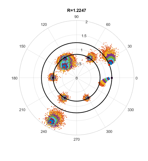
Figure 3: Root Neighborhoods for $7$ noise powers between $-22$dB and $-5$dB for $K=6$ Huffman zeros and $L-1=3$ channel zeros.

To derive such a quantized result we will exploit Rouché’s Theorem to bound the single root neighborhoods by discs, see e.g. [Mar77, Thm (1,3)].

Theorem 1 (Rouché).

Let ${\mathrm{X}}(z)$ and ${\rm{W}}(z)$ be analytic functions in the interior to a simple closed Jordan curve $C$ and continuous on $C$. If

$$|{\rm{W}}(z)|\leq|{\mathrm{X}}(z)|,\quad z\in C,$$ (78)

then ${\mathrm{Y}}(z)={\mathrm{X}}(z)+{\rm{W}}(z)$ has the same number of zeros interior to $C$ as does ${\mathrm{X}}(z)$.

The Theorem allows to prove that the zeros of polynomials are continuous functions of the coefficients, see [Mar77, Thm (1,4)]. However, to obtain an explicit robustness result for the zeros, we need a quantized version of the continuity, i.e., a Lipschitz bound of the root functions with respect to the $\ell_{\infty}/\ell_{2}$ norm. As simple closed Jordan curves we will consider the Euclidean circle and the disc as its interior, which will contain the single root neighborhoods. Let us define for $\alpha_{n}\in{\mathbb{C}}$ the closed Euclidean ball (disc) of radius $\delta>0$ and its boundary as

$$B_{n}(\delta)=B(\delta,\alpha_{n})=\left\{\left.z\in{\mathbb{C}}\rule[-2.5pt]{0.0pt}{10.0pt}\;\right|\;|z-\alpha_{n}|\leq\delta\right\}\quad,\quad C_{n}(\delta)=\left\{\left.z\in{\mathbb{C}}\rule[-2.5pt]{0.0pt}{10.0pt}\;\right|\;|z-\alpha_{n}|=\delta\right\}.$$ (79)

Let us consider an arbitrary polynomial (analytic function in ${\mathbb{C}}$) of order $N\geq 1$:

$${\mathrm{X}}(z)=\sum_{n=0}^{N}x_{n}z^{n}.$$ (80)

Then, its roots are functions of the polynomial coefficients ${\mathbf{x}}\in{\mathbb{C}}^{N+1}$ given by

$$\alpha_{n}=\alpha_{n}({\mathbf{x}})\quad,\quad n=1,\dots,N.$$ (81)

If the coefficients are disturbed by a vector ${\mathbf{w}}\in{\mathbb{C}}^{N+1}$, the maximal perturbation of the zeros should be bounded by

$$\max_{n}|\alpha_{n}({\mathbf{x}}+{\mathbf{w}})-\alpha_{n}({\mathbf{x}})|\leq\delta\cdot\left\|{\mathbf{x}}+{\mathbf{w}}-{\mathbf{x}}\right\|_{2}=\delta\cdot\left\|{\mathbf{w}}\right\|_{2},$$ (82)

where the bound $\delta=\delta(\epsilon,{\mathbf{x}})>0$ is a local Lipschitz constant for ${\mathbf{w}}\in B(\epsilon,{\mathbf{x}})$, which we want to derive. If the noise coefficient $w_{N}=-x_{N}$, i.e., the leading coefficient is vanishing, then we will set $\alpha_{N}({\mathbf{x}}+{\mathbf{w}})=0$, since the order of the perturbed polynomial would reduce to $N-1$. We are now ready to prove the following local Lipschitz bound. We use here the assumption that one zero is outside the unit circle, which is always the case for polynomials generated by autocorrelations.

Theorem 2.

Let ${\mathrm{X}}(z)\in{\mathbb{C}}[z]$ be a polynomial of order $N>1$ with simple zeros $\alpha_{1},\dots,\alpha_{N}\subset{\mathbb{C}}$ inside a circle of radius $R>1$ with minimal pairwise distance ${d_{\text{\rm min}}}>0$, i.e.

$${d_{\text{\rm min}}}:=\min_{n\not=k}|\alpha_{n}-\alpha_{k}|\quad,\quad R=\arg\max_{n}|\alpha_{n}|.$$ (83)

Let ${\mathbf{w}}\in{\mathbb{C}}^{N}$ with $\left\|{\mathbf{w}}\right\|_{2}\leq\epsilon$ be an additive perturbation on the polynomial coefficients ${\mathbf{x}}$ and $\delta\in[0,{d_{\text{\rm min}}}/2)$. Then the $n$th zero $\zeta_{n}$ of the disturbed polynomial ${\mathrm{Y}}(z)={\mathrm{X}}(z)+{\rm{W}}(z)$ lies in $B_{n}(\delta)$ if

$$\epsilon=\epsilon({\mathbf{x}},\delta)\leq\frac{|x_{N}|\delta({d_{\text{\rm min}}}-\delta)^{N-1}}{\sqrt{1+N}(R+\delta)^{N}}.$$ (84)

Remark. The minimal pairwise distance of the zeros is also called zero separation, see for example [Zip93, Sec.11.4].

Proof.

The proof is a quantized version of the proof in [Mar77, Thm (1,4)]. Let us define the error polynomial

$${\rm{W}}(z)=\sum_{n=0}^{N}w_{n}z^{n}.$$ (85)

By defining $\underline{{\mathbf{z}}}=(z^{0},z^{1},\dots,z^{N})^{T}$, we can upper bound the magnitude of ${\rm{W}}$ with the Cauchy-Schwarz inequality

$$|{\rm{W}}(z)|=|{\mathbf{w}}^{T}\underline{{\mathbf{z}}}|\leq\left\|{\mathbf{w}}\right\|_{2}\cdot\left\|\underline{{\mathbf{z}}}\right\|_{2}=\epsilon\cdot\Big{(}\sum_{n}|z^{n}|^{2}\Big{)}^{1/2}=\epsilon\cdot\Big{(}\sum_{n}|z|^{2n}\Big{)}^{1/2}=\epsilon\cdot f(|z|).$$ (86)

Since $f(r)$ is monotone increasing in $r>0$, the largest upper bound in $C_{m}(\delta)$ is attained at $z=|\alpha_{m}|+\delta$ and hence

$$f(|\alpha_{m}|+\delta)^{2}\leq\begin{cases}1+N\cdot(|\alpha_{m}|+\delta)^{2N}&,|\alpha_{m}|+\delta>1\\ 1+N\cdot(|\alpha_{m}|+\delta)^{2}&,|\alpha_{m}|+\delta\leq 1\end{cases}$$ (87)

By assumption it holds $R=|\alpha_{\text{\rm max}}|>1$ which gives us the universal upper bound

$$|{\rm{W}}(z)|\leq\epsilon\cdot\sqrt{1+N}(R+\delta)^{N}\quad,\quad z\in\bigcup C_{m}(\delta).$$ (88)

On the other hand, the magnitude of the original polynomial

$$|{\mathrm{X}}(z)| =|x_{N}|\prod_{n=1}^{N}|z-\alpha_{n}|\quad,\quad z\in C_{m}(\delta)$$ (89)

$$=|x_{N}|\prod_{n}|\alpha_{m}+\delta e^{i\theta}-\alpha_{n}|\quad,\quad\theta\in[0,2\pi)$$ (90)

can be lower bounded by using the reverse triangle inequality

$$\geq|x_{N}|\prod_{n}||\alpha_{m}-\alpha_{n}|-\delta|\geq|x_{N}|\delta\prod_{n\not=m}({d_{\text{\rm min}}}-\delta).$$ (91)

Hence we get for all $z\in\bigcup C_{n}(\delta)$:

$$|{\mathrm{X}}(z)|\geq|x_{N}|\delta({d_{\text{\rm min}}}-\delta)^{N-1}.$$ (92)

To apply Rouché’s Theorem, we have to show $|{\rm{W}}(z)|<|{\mathrm{X}}(z)|$ for all $z\in\bigcup C_{n}(\delta)$, which gives us the universal bound

$$\epsilon=\epsilon({\mathbf{x}},\delta)\leq\frac{|x_{N}|\delta({d_{\text{\rm min}}}-\delta)^{N-1}}{\sqrt{1+N}(R+\delta)^{N}}.$$ (93)

Since $\delta<{d_{\text{\rm min}}}/2$, all $B_{n}(\delta)$ are disjoint and ${\mathrm{Y}}(z)$ has exactly one zero in each $n$th ball $B_{n}(\delta)$ by Theorem (1). Note, that $x_{N}=x_{N}(\boldsymbol{\alpha})$ depends on the selected zeros and the normalization $\left\|{\mathbf{x}}\right\|=1$. ∎

Remark. Let us note, that the bound (93) does not increases with $\delta$ for fixed ${\mathbf{x}},R$ and ${d_{\text{\rm min}}}$, see Figure (4). This behaviour is due to the continuity of the zeros very unlikely and hence caused by the worst bound in (91). In Section (X) we will investiage in more detail the geometric structure of the zero placements, to obtain sharper stability bounds.

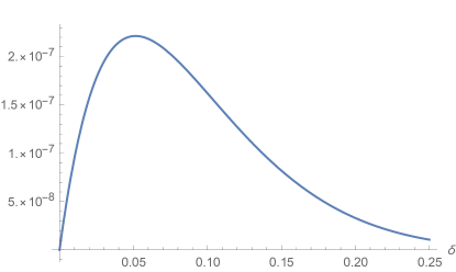
Figure 4: Noise bound (93) for fixed Radius $R=1.1$ and ${d_{\text{\rm min}}}=0.5$ over $\delta$.

Furthermore, if $|\alpha_{\text{\rm max}}|=\text{const}$ and $|x_{N}|=\text{const}$, then a maximal separation of the zeros yields to robustness against additive noise on the coefficients. Hence, if we place the zeros with maximal pairwise distance for fixed $R$, this suggests a good BER performance for the RFMD decoder. Moreover, by setting $\delta={d_{\text{\rm min}}}/2$ the bound (84) gives

$$\epsilon\leq\frac{|x_{N}|}{\sqrt{1+N}}\frac{{d_{\text{\rm min}}}^{N}}{2^{N}(|\alpha_{\text{\rm max}}|+{d_{\text{\rm min}}}/2)^{N})},$$ (94)

which is a upper threshold of the noise power under which no errors can occur. It can be seen that the noise bound increases if ${d_{\text{\rm min}}}$ increases, which again validates a larger zero separation.

For Huffman sequences with radius $R$ we obtain ${d_{\text{\rm min}}}=2R\sin(\pi/N)$ and hence (94) gives

$$\epsilon\leq\frac{1}{\sqrt{1+N}}\frac{1}{\sqrt{(R^{-2N}+1)}(1/\sin(\pi/N)+1)^{N}}.$$ (95)

Note, the bound becomes independent of $R$ if one zero is outside the unit circle and hence equal to $R$. A plot for different $N$ is given in Figure (5) for uniform radius $R_{\text{uni}}$ in (102).

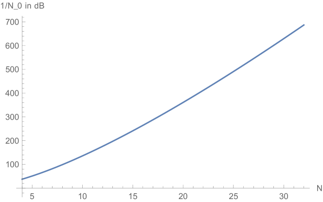
Figure 5: SNR bound (95) with $\delta=\delta_{\text{max}}$ for Huffman sequences over various dimensions $N$ and uniform radius $R_{\text{uni}}(N,1)$ in (102) allowing a perfect reconstruction.

Moreover, if $|\alpha_{\text{\rm max}}|=t{d_{\text{\rm min}}}/2$ for some $t\geq 1$ then we get

$$\epsilon\leq\frac{|x_{N}|}{\sqrt{1+N}(t+1)^{N}}.$$ (96)

However, an increase of $t$ means an increase of the largest root, which is coupled by the leading coefficient, due to a result of Cauchy

$$|\alpha_{\text{\rm max}}|\leq 1+\max_{k<N}{\Big{|}\frac{x_{k}}{x_{N}}\Big{|}}$$ (97)

see for example [Mar77, Thm.(27,2)]. If the energy of ${\mathbf{x}}$ is normalized this gives

$$|\alpha_{\text{\rm max}}|\leq 1+\frac{1}{|x_{N}|}\quad\Leftrightarrow\quad|x_{N}|\leq\frac{1}{|\alpha_{\text{\rm max}}|-1}$$ (98)

since $|\alpha_{\text{\rm max}}|>1$. Hence, if $|\alpha_{\text{\rm max}}|$ increases, the leading coefficient has to decrease and $\epsilon$ decreases rapidly, independently of ${d_{\text{\rm min}}}$.

Zeros of Random Channels

It is known, that a polynomial with i.i.d. Gaussian distributed coefficients has zeros concentrated around the unit circle. If the order $N$ goes to infinity, all zeros will be uniformly distributed on the unit circle with probability one, see for example [PY14] In fact, this even holds for other random polynomials with non Gaussian distributions, see [HN08]. This is an important observation, since it implies for fixed $K$ and hence $R$, that an increase of $L$ will concentrate the channel zeros on the unit circle, such that the channel zeros will not interfere with the codebook zeros, as long as $R$ is sufficiently large.

Remark. The analysis of the stability radius for a certain zero-codebook and noise power, allows in principle an error detection for the RFMD decoder. Here, an error for the $l$th zero can only occur if the noise power is larger than the RHS of (84). However, in the presence of the channel ${\mathbf{h}}$, we can adopt the dimension $N$ and $x_{N}\rightarrow x_{K}h_{{L}-1}$, if we assume the absolute values of the zeros of ${\mathrm{H}}(z)$ are not larger than $R$. The minimal distance might be fulfilled with a certain probability. A precise analysis of the expectation might lead to upper bounds of the bit error probabilities of the RFMD decoder, which will be a future research topic. Note also, that is not clear, what the distribution of the disturbed zeros $\zeta_{n}$ are. If they would be Gaussian known results of polar quantization might apply, see for example [NCTH14]. Huffman sequences for $R=1$ are uniformly concentrated on a unit circle and show the best noise robustness Figure (7(a)).

Figure 6: Zero Constellations, which allows largest non-overlapping uniform root-neighborhood discs for the Huffman BMOCZ scheme with largest radius $\delta_{\text{max}}={d_{\text{\rm min}}}/2$.

VII-A Radius for Huffman BMOCZ Allowing Largest Uniform Root Neighborhood Discs

To ensure robustness of a zero-based decoding against additive noise we need to place the zero-constellations carefully, as will be pointed out in more detail in Section (VII). Theorem (2) below suggest for Huffman polynomials to place the zero-set $\mathscr{Z}$ with maximal pairwise distance under the constraint of being uniformly spaced conjugate-reciprocal pairs. Here the distance between conjugated pairs is given by

$$d_{cp}=R-R^{-1}$$ (99)

and the distance between next-neighbor pairs for the smaller radius $R^{-1}$ by

$$d_{nn}=2R^{-1}\sin(\pi/{K}).$$ (100)

Setting both distances equal, yields a zero-set $\mathscr{Z}$ with maximal minimal pairwise distance ${d_{\text{\rm min}}}$, see Figure (6).

However, simulations of perturbed Huffman polynomials, see Figure (7), show a strong dependence of the root neighborhood radius. In fact, an increasing of $R$ yields to an increasing of the root neighborhood radius $\delta$, which obtains its minimum if $R=1$. However, if $R$ gets to small, the root neighborhood of the reciprocal-pairs will overlap. To address this problem we will introduce $\lambda\geq 1$ as a scaling parameter which yields to

$$\lambda d_{cp}=d_{nn}\quad \Leftrightarrow\quad\lambda(R^{2}-1)=Rd_{nn}=2\sin(\pi/{K})$$ (101)

$$\Rightarrow\quad R_{\text{uni}}(K,\lambda)=\sqrt{1+\frac{2}{\lambda}\sin(\pi/{K})}\simeq\sqrt{1+\frac{2\pi}{{K}}},$$ (102)

which is bounded between

$$1+\frac{\pi}{\lambda{K}}\leq R_{\text{uni}}(K)\leq e^{\pi/2\lambda{K}}.$$ (103)

Therefore, we will in Section (VII) investigate the radius dependence in more detail. Finding the optimal radius for Huffman sequences yielding to the optimal Voronoi cells $\mathfrak{D}_{k}$ is in fact a quantization problem, see for example [KJ17]. Note, that the zeros for Huffman BMOCZ are not the centroids of the Voronoi cells, which suggest a much more complex metric for an optimal quantization, see Figure (7). From the simulation of the BER performance we observed $\lambda\simeq 2$, which might be also $L$ dependent.

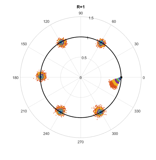
(a) Radius $R=1$ with $\lambda=\infty$.

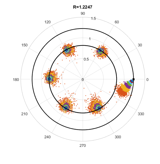
(b) Radius $R=1.2247$ with $\lambda=2$.

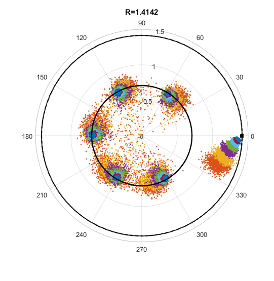
(c) Radius $R=1.4142$ with $\lambda=1$.

Figure 7: Simulation of $7$ different SNR values from $22$dB to $5$dB for a fixed Huffman sequence with $N=6$ over different radii.

VII-B PAPR for Huffman Sequences with Uniform Radius

From (27) we get for the magnitudes

$$|x_{K}|^{2},|x_{0}|^{2}\in\Big{[}\frac{1}{{1+R^{2{K}}}},\frac{1}{{1+R^{-2{K}}}}\Big{]},$$ (104)

where the maximum is attained if ${\mathbf{b}}={\mathbf{0}}$ or ${\mathbf{b}}={\mathbf{1}}$, the all zero or all one bit vector. By noting that the first and last coefficient magnitude (27) exploit a symmetry for $2\left\|{\mathbf{b}}\right\|_{1}$ and $K-2\left\|{\mathbf{b}}\right\|_{1}$, we only have to average for uniform bit distribution over $\left\|{\mathbf{b}}\right\|_{1}\in\{0,\dots,K/2\}$ (assuming $K$ even), which gets :

$${\mathbb{E}[\left\|{\mathbf{x}}\right\|_{\infty}^{2}]} =\frac{1}{2^{K/2}}\frac{1}{R^{2K}+1}\sum_{n=1}^{2^{K/2}}R^{-2\sum_{k=1}^{K/2}b_{k}^{(n)}}=\frac{1}{2^{K/2}}\frac{1}{R^{2K}+1}\sum_{m=0}^{{K/2}}\binom{K/2}{m}R^{-2m}$$ (105)

$$=\left(\frac{1+R^{-2}}{2}\right)^{\frac{K}{2}}\frac{1}{R^{2K}+1}$$ (106)

Since the Huffman sequences have all unit energy, the peak-to-average-power ratio is for the optimal radius $R=R_{\text{uni}}(K,1)$ in (102) for large $K$

PAPR $$=({K}+1)\frac{{\mathbb{E}[\left\|{\mathbf{x}}\right\|_{\infty}^{2}]}}{{\mathbb{E}[\left\|{\mathbf{x}}\right\|_{2}^{2}]}}=\frac{({K}+1)((1+R^{-1})/2)^{K/2}}{R^{2{K}}+1}{\simeq}\frac{{K}+1}{(1+2\pi/{K})^{{K}}+1}$$ (107)

$${\leq}\frac{{K}+1}{2+2\pi}\simeq\frac{{K}+1}{8.28}\simeq{K}/9,$$ (108)

which is typically for a multi-carrier system, such as OFDM [BF11].

VIII Numerical Simulations

We simulated with MatLab 2017a the bit-error-rate (BER) over the rSNR (5) for ${L}$ Rayleigh fading multipaths with power delay profile exponent $p<1$.

In the simulation, we scaled the transmit signals ${\mathbf{x}}$ by $\sqrt{N}$ and the channel by $\sqrt{1/{\mathbb{E}[\left\|{\mathbf{h}}\right\|_{2}^{2}]}}$, such that the received average power will be normalized and equal to the transmitted average power, independent of $N,{L}$ and $\underline{\mathbf{p}}$. Hence we obtain ${\text{rSNR}}={\text{SNR}}=1/N_{0}$. The energy per bit is then

$$E_{b}=\frac{N}{{L}}=R_{b}^{-1},$$ (109)

which is equal to the inverse of the bit rate $R_{b}$ per symbol time. Hence, the SNR per bit is

$$\frac{E_{b}}{N_{0}}=\frac{1}{R_{b}\cdot N_{0}}=\frac{{\text{SNR}}}{R_{b}}$$ (110)

see for example [PS08, pp.97].

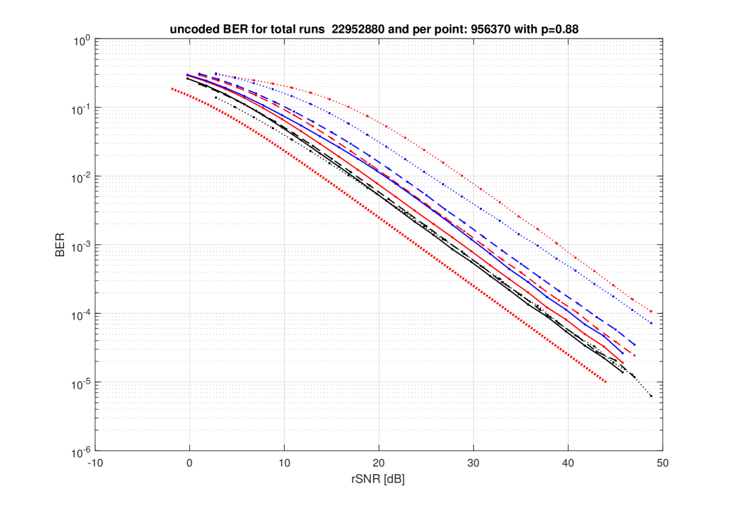
(a) Bit error results over SNR for $p=0.88$

(b) Bit error results over $E_{b}/N_{0}$ for $p=0.88$

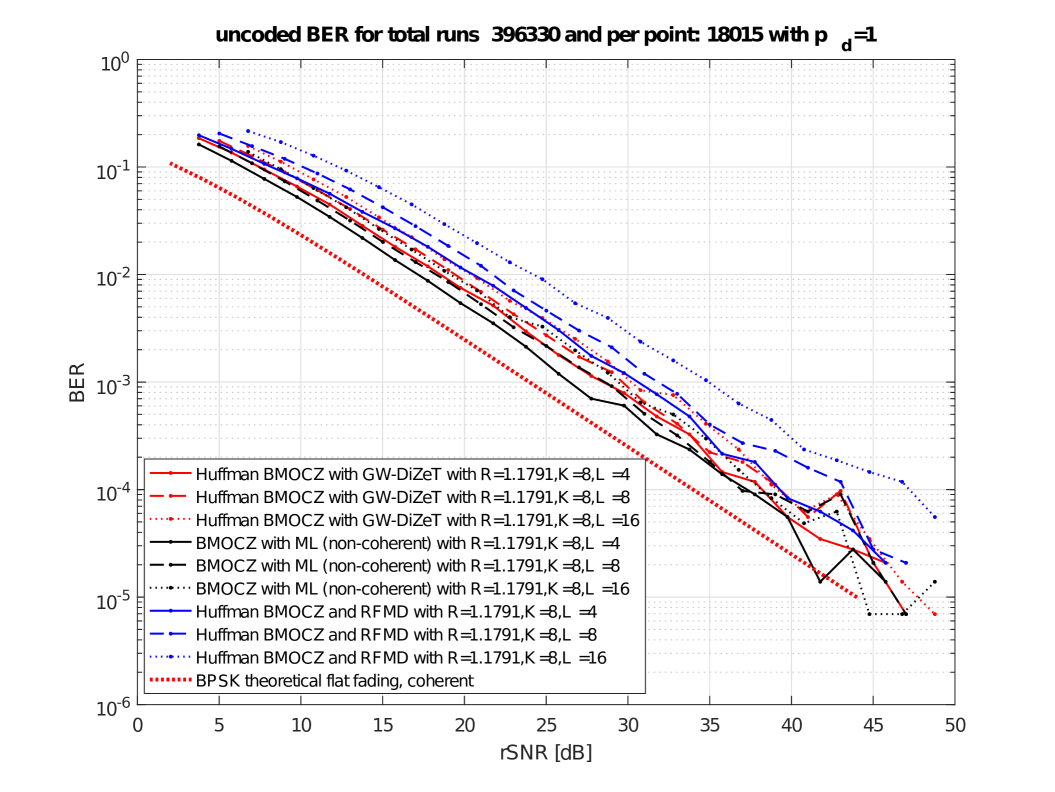
(c) Bit error results over SNR for $p=1$.

(d) Bit error results over $E_{b}/N_{0}$ for $p=1$.

Figure 8: Huffman BMOCZ with RFMD, GW-DiZeT and ML (with known $N_{0}$ and $\underline{\mathbf{p}}$) decoder for ${K}=8$ and channel length ${L}=4,8$ and $16$ under different power delay profiles $p$.

As an ultimate benchmark in all simulations, we will compare to the coherent case, where the frequency selective channel is modulated by OFDM with a binary phase shift keying (BPSK). Transforming the linear convolution for i.i.d. Gaussian CIR in time domain to the frequency domain, yields to $N$ parallel flat fading channels. Assuming a sequential block transmission, the cyclic prefix, allows to communicate $N$ bits per channel use and results therefore in coherent BPSK flat fading. The BER for BPSK over a flat fading channel $h_{0}=|h_{0}|e^{i\phi}$, with known phase $\phi$ and ${\mathbb{E}[|h_{0}|^{2}]}=1$ is equivalent to the bit error probability (one bit per symbol duration) given by

$$P_{e}=\frac{1}{2}\left(1-\sqrt{\frac{E_{b}{\mathbb{E}[|h_{0}|^{2}]}/N_{0}}{1+E_{b}{\mathbb{E}[|h_{0}|^{2}]}/N_{0}}}\right)=\frac{1}{2}\left(1-\sqrt{\frac{{\text{rSNR}}}{1+{\text{rSNR}}}}\right)$$ (111)

since $\sigma_{h}^{2}=1$ we have in Figure (10) $E_{b}/N_{0}=E_{b}{\mathbb{E}[|h_{0}|^{2}]}/N_{0}={\text{rSNR}}$, pictured as a thick doted red curve. The BPSK coherent flat fading can be seen as the best binary signaling scheme performance if no multi-path diversity is exploit (no outer codes). Note, that our scheme prevent is therefore robust against inter-symbol-interference (ISI), given by superposition of overlapping symbols due to the multipath delays. It is still unclear how to exploit fully the multipath diversity gain in one-shot at the receiver without knowledge of the CIR. However, the DiZeT decoder performs very close to the ML decoder and coherent uncoded OFDM with BPSK, see Figure (8). Note, all simulated BER curves are for uncoded bits. In Figure (9) the BER for the SDP denoising (65) with the estimate channel autocorrelation via (71) are simulated for $K=8$ and $L=4$ with flat power delay profile. The denoised signal ${\hat{\mathbf{x}}}$ from the SDP is then either decoded by the GW-DiZeT decoder or the RFMD decoder. The results show a $2$dB lose compared to GW-DiZeT without denoising. The reason for the performance lose is first in the bad estimation of the channel autocorrelation and secondly due to the simultaneously denoising of the channel and signal. Since the SDP does not emphasize the signal reconstruction quality, the quality in signal recovery is in sum worse as for the direct decoding approaches. However, the knowledge of the channel might help for other purposes.

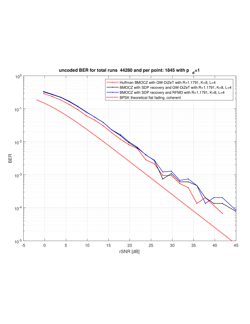
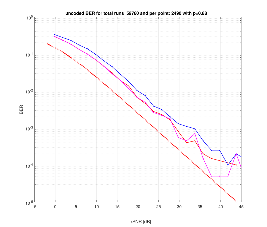
Figure 9: GW-DiZeT decoder versus SDP denoising with GW-DiZeT and RFMD decoding.

IX Comparison to Training Schemes

We will compare our noncoherent BMOCZ scheme to noncoherent QPSK with pilot signaling. Considering one-shot scenarios, there are not many noncoherent comparisons possible in this scenario. We refer the reader to [JHV15],[Cho18] and [FHV13] based on self-coherent OFDM schemes. However, our proposed Huffman BMOCZ schemes outperforms their BER performance. We assume in the simulations the following scenario

• Channel is time-invariant for $N$ time-instants

• Receive duration is $N={K}+{L}$

• Block length of transmitted signal is ${K}+1$

• We have independent Rayleigh distributed channel gains $h_{l}\in\mathcal{CN}(0,p^{l})$ with $p\leq 1$.

• After each block transmission the CIR can change arbitrary, e.g., caused by a fast-varying channel or due to a sporadic one-shot communication, where the next block message might occur much later, such that the channel state and user position can change drastically, resulting in fully uncorrelated CIRs.

Note, the maximum-likelihood (ML) detection is equal to the maximum a posteriori detection (MAP), if the channel is known. If we do joint ML over ${\mathbf{x}},{\mathbf{h}}$ then the ML and LS would also be the same, but this requires blind deconvolution, see [MMF98, (12-16)]. We will compare to the following scenarios

1. BPSK and full channel knowledge (coherent) by using . Zero-forcing (ZF) and hard thresholding bit wise

   $$m_{k}=\begin{cases}1,\operatorname{Re}({\hat{\mathbf{x}}}_{k})>0\\ 0,\operatorname{Re}({\hat{\mathbf{x}}}_{k})<0\end{cases}\quad,\quad{k}=1,2,\dots,{K}$$ (112)

2. QPSK with ${L}$ pilots. Here we assume that ${K}=2{L}$. We decode by separating Real and Imaginary part

   $$m_{k}=\begin{cases}1,\operatorname{Re}({\hat{\mathbf{x}}}_{k})>0\\ 0,\operatorname{Re}({\hat{\mathbf{x}}}_{k})<0\end{cases}\quad,\quad m_{{k}+{L}}=\begin{cases}1,\operatorname{Im}({\hat{\mathbf{x}}}_{k})>0\\ 0,\operatorname{Im}({\hat{\mathbf{x}}}_{k})<0\end{cases}\quad,\quad{k}=1,2,\dots,{K}$$ (113)

   This follows form the minimum distance decoder, see [LM93, (7.25)].

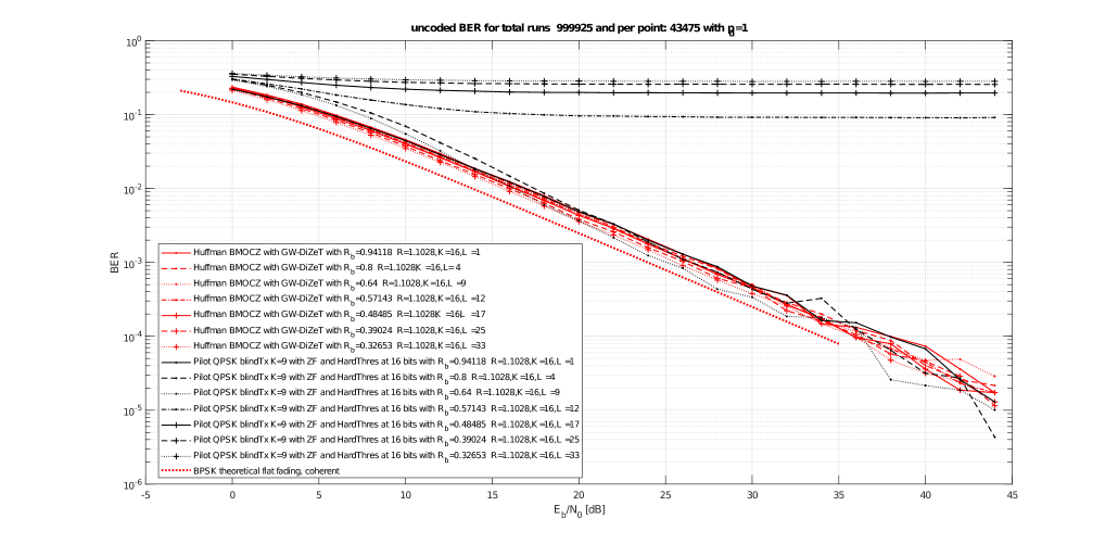
Figure 10: Pilot based QPSK in time domain versus Huffman BMOCZ with $p=1$ for ${K}=16$ and ${L}=1,4,9,12,17,25,33$.

Interesting scenarios for the BMOCZ scheme are distributed wireless sensor networks which require

• Low-Power (transmitter and receiver)

• Low-Latency

• No feedback and no channel information at transmitter

• Short block-length, ${K}\simeq{L}$

• One-shot communication, channel is used only once, sporadic in time

If ${K}<{L}$ there is no way to learn the channel with pilots in one shot. Moreover, the low-power assumption is not suitable to use energy detector if we need to transmit more than $1$ bit. Higher order MOZ modulation might be also considered. This constraints, rule out

• CDMA: usually requires ${K}\gg{L}$, [TV05, p.92]

• Clasical ODFM: needs channel for decoding. Hence, we could assume again ${\mathbf{x}}={\mathbf{u}}+{\mathbf{d}}$ And in $\hat{{\mathbf{d}}}$ using QAM. for example QPSK.

The BMOCZ scheme does not need channel length knowledge at the transmitter! On the other hand, any pilot data needs assumption on the channel length. If the pilots are to short, it is impossible to estimate exactly the channel, even in the noiseless case. We will investigate a scenario, where we blind transmit with $P=\lfloor{L}/2\rfloor$ pilots and $D=P$ data and receive only ${L}+{L}$ taps, regardless of the true channel length ${L}$. Hence, either we take to much sample or to less at the receiver. This will affect the performance of pilot-based schemes, which we simulated for QPSK and OFDM, see Figure (10). Here, the BER performance suffers dramatically if the channel length at the transmitter is underestimated, rendering a reliable communication impossible. However, the BMOCZ decoder depends heavily of the maximal channel length $L$. It can be seen in the simulation, that an overestimating of $L$ (fast decreasing power profile) is not affecting the BER performance much, see Figure (8(a)) and Figure (8(b)).

The GW-DiZeT decoder demands no complexity at all and allows with the DFT an easy and probably analog realization (using delayed amplified circuits). The complexity at the transmitter consist of a fixed codebook of size $2^{K}$ in ${\mathbb{C}}^{{K}+1}$ dimensions.

X Sharper Robustness Analysis for BMOCZ Codebooks by Exploiting the Geometric Zero Structure

We will in this section investigate the geometric structure of the zeros to improve the robustness of normalized polynomials against additive noise on its coefficients, sometimes also referred to the conditioning of a polynomial. This is not to mistaken with the notion of stable polynomials or Hurwitz stability, which refers to the property that all zeros are located in the positive half-plane, see for example [Fis08, Cha.21]. As we saw in the analysis of Theorem (2), a large pairwise distance as well as a large leading coefficient guarantee a robustness against additive noise. For polynomials generated by autocorrelations, we will have zeros in conjugate-reciprocal pairs and if we upper bound the largest zero, we force the zeros in a ring or annulus around the unit circle, which will exclude the extreme cases in the zero displacement, see Figure (11). It turns out that the Euclidean metric, as used in the RFMD decoder might be reasonable for zeros near the unit circle. Indeed, for Huffman Polynomials with uniform radius, the root neighborhoods can be bounded by disjoint uniform discs, see Figure (7). However, the first zero on the real line, seem to disturb non uniform. This might be due to discontinuity of the real valued zero on the positive half plane (winding number). A more careful analysis of the exact root neighborhood grow behaviour will be investigated in a follow up paper. Since we want to keep the root neighborhoods disjoint, the root neighborhoods should not exceed a radius $\delta$ which is larger then half the minimal pairwise distance. This in fact, leads to a circle packing problem in the plane, which is know to be most dense if the circle centroids are placed on a hexagonal lattice, see Figure (11(a)).

(a) Hexagonal packing in an annulus, worst constellation red, best constellation blue.

(b) Densest packing inside the ring, worst case.

Figure 11: Homogeneous Circle Packing in an annulus.

The idea is to place $N$ zeros in a Ring ${\mathscr{R}}={\mathscr{R}}(R)$ of area $|{\mathscr{R}}|$ with minimal pairwise distance ${d_{\text{\rm min}}}$. The bound in (91) is actually a lower bound of the geometric mean of all zeros distances. Hence, the robustness bound depends not only on the minimal pairwise distance but also on their geometric structure. In fact, the densest packing of the $N$ zeros will yield to the smallest geometric mean of the distances and therefore result in the worst stability bound, see Figure (11). Furthermore, the maximal amount of zeros in the ring is bounded by the spherical circle packing problem. The exact amount is unsolved for arbitrary ${d_{\text{\rm min}}}$ even if the set is the unit disk. The problem is usually known as the density packing problem, where the density of placing $N$ equal circles of radius ${d_{\text{\rm min}}}$ in the ring ${\mathscr{R}}$ is given by

$$D=N{d_{\text{\rm min}}}^{2}\pi 4|{\mathscr{R}}|$$ (114)

One bound on the maximal number $N$ of circles is given by Fejer Toth as

$$N\leq\frac{\pi(R^{2}-R^{-2})}{{d_{\text{\rm min}}}^{2}\sqrt{12}}$$ (115)

see for example [GT00].

X-A Revised Proof of Theorem (2)

The main idea of the proof relies on the use of Rouches Theorem (1), by controlling for each $m=1,2,\dots,N$ the modulus of the noise polynomial on the single root neighborhood circle bounds

$$|{\rm{W}}(z)|\leq|{\mathrm{X}}(z)|\quad,\quad z\in C_{m}(\delta).$$ (116)

By choosing the radius $\delta$ small enough, such that no overlap of the single root neighborhoods occur, a separation by the RFMD decoder will be always successful (no channel zeros), guaranteeing an error free decoding. Since we want to hold this for every noise polynomial generated by $\left\|{\mathbf{w}}\right\|_{2}\leq\epsilon$ we have to satisfy

$$\max_{\left\|{\mathbf{w}}\right\|\leq\epsilon}\max_{z\in C_{m}(\delta)}\frac{|{\rm{W}}(z)|^{2}}{|{\mathrm{X}}(z)|^{2}}\leq 1.$$ (117)

Note, that ${\mathrm{X}}(z)$ has no zeros on $\bigcup C_{m}(\delta)$, hence we can divide. Let us define $\underline{{\mathbf{z}}}=(z^{0},z^{1},\dots,z^{N})^{T}$, where we set $0^{0}=1$. We will upper bound the magnitude of ${\rm{W}}$ by using Cauchy-Schwarz

$$|{\rm{W}}(z)|^{2}=|{\mathbf{w}}^{T}\underline{{\mathbf{z}}}|^{2}\leq\left\|{\mathbf{w}}\right\|_{2}^{2}\cdot\left\|\underline{{\mathbf{z}}}\right\|_{2}^{2}=\epsilon^{2}\cdot\sum_{n=0}^{N}|z|^{2n}.$$ (118)

Since the noise ${\mathbf{w}}$ is in the ball with radius $\epsilon$, all directions can be chosen and we achieve always equality in (118). Hence, (117) is equivalent to

$$\epsilon^{2}\leq\frac{1}{\max_{z\in C_{m}(\delta)}\frac{\sum_{n}|z|^{2n}}{|{\mathrm{X}}(z)|^{2}}}=\min_{z\in C_{m}(\delta)}\frac{|{\mathrm{X}}(z)|^{2}}{\sum_{n}|z|^{2n}}=\min_{z}f_{m}(z)$$ (119)

By using $z=\alpha_{m}+\delta e^{i\theta}$ for some $\theta\in[0,2\pi)$ we need to find a tight lower bound of

$$f_{m}(\theta):=\frac{|{\mathrm{X}}(\alpha_{m}+\delta e^{i\theta})|^{2}}{\sum_{n}|\alpha_{m}+\delta e^{i\theta}|^{2n}}=|x_{N}|^{2}\frac{\prod_{n}|\alpha_{m}+\delta e^{i\theta}-\alpha_{n}|^{2}}{\sum_{n}|\alpha_{m}+\delta e^{i\theta}|^{2n}}.$$ (120)

Since we are searching for a uniform radius $\delta$ which keeps all root neighborhoods disjoint, we search for the worst $\alpha_{m}$. The only information of the zeros we have is the minimal pairwise distance ${d_{\text{\rm min}}}$ and the smallest and largest moduli $R^{-1}$ resp. $R$, we define therefore

$${\mathcal{A}}:=\left\{\left.\alpha=\{\alpha_{1},\dots,\alpha_{N}\}\rule[-3.07999pt]{0.0pt}{11.71774pt}\;\right|\;\;\forall\;n:R\geq|\alpha_{n}|\geq R^{-1},{d_{\text{\rm min}}}\leq\min_{m\not=n}|\alpha_{m}-\alpha_{n}|\right\}.$$ (121)

Note, ${\mathcal{A}}$ is a compact set. The leading coefficient $x_{N}$ depends on all zeros and the height of the polynomial, given by

$$\left\|{\mathrm{X}}\right\|_{2}:=\left\|{\mathbf{x}}\right\|_{2}=\sqrt{\sum_{n=0}^{N}|x_{n}|^{2}}.$$ (122)

We chose here the Euclidean norm as the height, since we are interested in SNR performance. Hence, we define the set of all allowable normalized polynomials with zeros in ${\mathcal{A}}$ as

$$\mathscr{P}=\mathscr{P}({\mathcal{A}}):=\left\{\left.{\mathrm{X}}(z)=\sum_{n=0}^{N}x_{n}z^{n}=x_{N}\prod_{n}(z-\alpha_{m})\rule[-2.5pt]{0.0pt}{10.0pt}\;\right|\;\left\|{\mathbf{x}}\right\|_{2}=1,\alpha\in{\mathcal{A}}\right\}.$$

This brings us to the following optimization problem

$$f(\mathscr{P})=\min_{{\mathrm{X}}\in\mathscr{P}}|x_{N}|^{2}\min_{m}\min_{\theta}\frac{\prod_{n}|\alpha_{m}+\delta e^{i\theta}-\alpha_{n}|^{2}}{\sum_{n}|\alpha_{m}+\delta e^{i\theta}|^{2n}}.$$ (123)

The modulus of the leading coefficient can be lower bounded for normalized polynomials by

$$2^{-N}\leq 2^{-N}\left\|{\mathbf{x}}\right\|_{1}\leq|x_{N}|\prod_{n=1}^{N}\max\{1,|\alpha_{n}|\},$$ (124)

see for example [Mah60] or [Zip93, Prop.86]. Note, this bound is not very tight for simple zeros with large minimal pairwise distance. If all zeros are inside the unit circle, this results in the largest lower bound and if all zeros are on the outside radius this results in the lowest bound, i.e.,

$$2^{-N}\leq|x_{N}|\quad,\quad{(2R)}^{-N}\leq|x_{N}|.$$ (125)

Using the worst case bound allows to eliminate the height constraint

$$f(\mathscr{P})\geq(2R)^{-N}\min_{\alpha\in{\mathcal{A}}}\min_{m}\min_{\theta}\frac{\prod_{n}|\alpha_{m}+\delta e^{i\theta}-\alpha_{n}|}{\sqrt{\sum_{n}|\alpha_{m}+\delta e^{i\theta}|^{2n}}}$$ (126)

which is necessary to leverage the problem to a pure geometric problem. Let us assume $\alpha_{\hat{m}}=\rho e^{i\phi}$ is the zero selection for which there exists a $\theta$ which obtains the minimum. Then, we can rotate all zeros by $e^{-i\phi}$, since it will not change their modulus nor their pairwise distances and hence be lying in ${\mathcal{A}}$ (rotation invariant). Since the numerating of $\alpha_{n}$ is arbitary, we can just chose $\alpha_{\hat{m}}=\alpha_{1}=\rho$. Hence, we can omit the minimization over $m$ since we minimize over all $N-1$ zeros and $\alpha_{1}\in[R^{-1},R]$. This brings us to the non-convex geometric problem

$$\min_{\alpha\in{\mathcal{A}}}f(\alpha)=\min_{\alpha,\alpha_{1}\in[R^{-1},R]}\min_{\theta}\frac{\prod_{n}|\alpha_{1}+\delta e^{i\theta}-\alpha_{n}|}{\sqrt{\sum_{n}|\alpha_{1}+\delta e^{i\theta}|^{2n}}}.$$ (127)

The nominator is independent of the other $N-1$ zeros, and obtains its maximum for $|R+\delta|$. It can be seen that the numerator, will not yield the global minimal constellation if we place the $N-1$ zeros around $\alpha_{1}=R$, for $N\geq 2$, due to the restriction of the ring. However, it is geometrical not obvious which $\alpha_{1}$ will yield the global minimum of $f$. Therefore, we lower bound the nominator in $f(\alpha)$, independently of the numerator, by the geometric formula for the worst case

$$f(\alpha)\geq\sqrt{\frac{(R+\delta)^{2}-1}{(R+\delta)^{2N}-1}}g(\alpha)\quad\text{ with }\quad g(\alpha)=\min_{\theta}g(\alpha,\theta)=\prod_{n=1}^{N}|\alpha_{1}+\delta e^{j\theta}-\alpha_{n}|.$$ (128)

Now, the minimization over the zeros reduces to the densest packing of $\alpha_{2},\dots,\alpha_{N}$ around $\alpha_{1}$, since the geometric mean $g(\alpha)^{1/n}$ of the distances decreases if each distance decreases. If $N=7$, the densest packing is the hexagon inscribed in a radius ${d_{\text{\rm min}}}$ with one zero at its centroid, see Figure (11(b)). For arbitrary $N$ this is the well known circle packing problem, also known as the “penny packing“ problem. However, it is not obvious if the optimal $z$ lies on the circle around the centroid or on the circle around the vertices. If $\alpha_{1}$ is the centroid, then we can show by Theorem (4) that extremal $z$’s will lie at crossing of the circle with the line between origin and one vertex. Since we want to maximize the nominator, the $z$ which lies on the real axis, right from the centroid, will therefore obtain the minimal value of $f$. If $\alpha_{1}$ is one of the vertices, then we need to show that $z$ does not achieve a smaller product distance. Unfortunately, we can not prove this analytically and formulated this as Conjecture (1) in Appendix (A).

If the conjecture holds, then the idea is to consider nested polygons (honeycombs) as the worst case zero configuration, to derive a lower bound for (128). Each $n$th honeycomb consist then of $6n$ points, placed on $n$ hexagons rotated accordingly, see Figure (11(b)). By Theorem (4), the optimal point $z=\alpha_{1}+\delta e^{j\theta}$ for the inner hexagon is achieved for $\theta=0$. This gives us a lower bound for the minimal product distance for the $1$st hexagon inscribed in a circle with radius $r_{1}={d_{\text{\rm min}}}$ as

$$\prod_{k=1}^{6}|\delta-\alpha_{n_{k}^{(1)}}|^{2}\geq|r_{1}^{6}-\delta^{6}|^{2}=r_{1}^{2\cdot 6}\cdot{\underbrace{|1-(\frac{\delta}{{d_{\text{\rm min}}}})^{6}|}_{=c^{6}(\delta,{d_{\text{\rm min}}})}}^{2}\geq r_{1}^{12}\cdot c^{12}$$ (129)

where we assume ${\delta}/{{d_{\text{\rm min}}}}\leq 1/2$, since $\delta<{d_{\text{\rm min}}}/2=r_{1}/2$. The radius for the $n$th hexagon is $n{d_{\text{\rm min}}}$, where on the $n$th honeycomb the $6n$ zeros, are the vertices of $n$ rotated hexagons. The smallest radius $r_{n}$ is given hereby with the law of cosine as

$$r_{n}=\sqrt{{d_{\text{\rm min}}}^{2}(1+n^{2}-2n\cos(\pi/3))}={d_{\text{\rm min}}}\sqrt{1+n^{2}-n}\geq{d_{\text{\rm min}}}(n-1)$$ (130)

for $n\geq 2$, see Figure (11(b)). If $n=1$ we set $r_{1}={d_{\text{\rm min}}}$. Then we get for the product of distance of the $n$th honeycomb for $n\geq 2$

$$p^{(n)}=\prod_{k=1}^{6n}|\delta-\alpha_{n_{k}}|^{2}=\prod_{m=1}^{n}\prod_{k=1}^{6}|\delta-\alpha_{n_{k}^{(m)}}|^{2}\geq\prod_{m}(c{d_{\text{\rm min}}}(n-1))^{12}=(\tilde{d}_{\text{min}}(n-1))^{12n}$$ (131)

with $\tilde{{d_{\text{\rm min}}}}=c{d_{\text{\rm min}}}$. If we have $n_{\text{max}}$ nested honeycombs we have up to

$$N=1+\sum_{n=1}^{n_{\text{max}}}6n=1+3n_{\text{max}}(n_{\text{max}}+1)$$ (132)

zeros packed, which gives the lower bound

$$n_{\text{max}}=\lceil\sqrt{\frac{4N-1}{12}}-\frac{1}{2}\rceil$$ (133)

of nested honeycombs, yielding to

$$g(\alpha) \geq\delta^{2}\left(\tilde{d}_{\text{min}}\prod_{n=2}^{n_{\text{max}}}(\tilde{d}_{\text{min}}(n-1))^{n}\right)^{12}=\delta^{2}\left(\tilde{d}_{\text{min}}\prod_{n=1}^{n_{\text{max}}-1}\tilde{d}_{\text{min}}^{n}n^{n+1}\right)^{12}$$ (134)

$$=\delta^{2}\left(\tilde{d}_{\text{min}}\tilde{d}_{\text{min}}^{\frac{n_{\text{max}}(n_{\text{max}}-1)}{2}}\prod_{n=1}^{n_{\text{max}}-1}n^{n+1}\right)^{12}$$

$$\geq\delta^{2}\tilde{d}_{\text{min}}^{\ 6(n_{\text{max}}^{2}-n_{\text{max}}+2)}\cdot[(n_{\text{max}}-1)!H(n_{\text{max}}-1)]^{12},$$ (135)

where the last factor is the hyperfactorial $H(n_{\text{max}}-1)=\prod_{n=1}^{n_{\text{max}}-1}n^{n}$. Note, that we had to add the distance square $|\alpha_{1}+\delta e^{i\theta}-\alpha_{1}|^{2}=\delta^{2}$ of the centroid zero $\alpha_{1}$. Combining (126) ,(127) and (128) would yield the final noise bound.

X-B Noise Bounds for Huffman Polynomials

Note, the noise energy bound (119) is deterministic and not in mean. First of all, for fixed $R$ and ${d_{\text{\rm min}}}$ the number $N$ of zeros we can place in the ring ${\mathscr{R}}$ is bounded by (115). We plotted in Figure (12) the noise power bound for fixed $N$ over various $R$. Here, we set ${d_{\text{\rm min}}}=\sqrt{\pi(R^{2}-R^{-2})/N\sqrt{12}}$ and assume that all zeros are place in a circle of area $\pi(R^{2}-R^{-2})$ with center at $R$. This is the worst packing for $N$ zeros. However, it can be seen that the bound is not very sharp if $N$ increases. We assume that Huffman sequences, placed on vertices of two $N-$gons are the best case. However, the optimal radius in the sense of maximal noise robustness for a fixed $N$ is still unknown. Nevertheless, the simulation and analysis suggest that a radius close to the optimal might be given if the uniform circle neighborhoods touching each other, see Figure (6) and Figure (13(b)) for a simulation of $N=6$. In fact, the root-neighborhoods are directed, depending on the particular choice of the other zeros. Hence, in average, the root-neighborhoods will more likely be bounded by an ellipse. Also the outside root-neighborhoods have larger radii than the insides, which suggest also a heterogeneous neighborhoods.

Figure 12: Worst case noise bounds for various $N$ and densest packing in circles of radius $R$.

Theorem 3 (Noise Bound for Huffman BMOCZ).

Let $N=4M$ for some $M\geq 3$ and $\mathscr{C}(N,R)$ be the set of normalized Huffman sequences in ${\mathbb{C}}^{N+1}$ with radius $R>1$. Then the minimal pairwise distance is given by

$${d_{\text{\rm min}}}=2R^{-1}\sin(\pi/N)$$ (136)

and the maximal noise power which guarantees root neighborhoods in circles of radius $\delta\in[0,{d_{\text{\rm min}}}/2)$ is given by

$$N_{0} \leq\frac{1}{R^{8M}+1}\frac{(R+\delta)^{2}-1}{(R+\delta)^{8M}-1}\cdot R^{2-4M}\delta^{4}(2R^{-1}\sin(\pi/N)-\delta)^{4}\prod_{m=3}^{M}m^{4}\cdot$$ (137)

$$\quad\quad\left(\frac{\sin(2\pi/N)-\sin(4\pi/N)-2\sin(\pi/N)}{2(1-\sin(2\pi/N))}\right)^{4M-12}$$ (138)

The worst case Huffman sequence is given by all zero inside the unit circle except one.

Remark. If Conjecture (1) holds then we would get the noise power bound

$$N_{0}\leq\frac{R^{-3N}}{R^{-2N}+1}\cdot\frac{(R+R^{-1}\sin(\pi/N))^{2}-1}{(R+R^{-1}\sin(\pi/N))^{2N}-1}\cdot(1-(1-\sin(\pi/N))^{N})^{2}$$ (139)

which yields to the bounds over $N$ in Figure (13(b)) for $\delta=\delta_{max}=R^{-1}\sin(\pi/N)$. The red line shows the bound for a radius where all root neighborhoods remain disjoint.

(a) Root neighborhood radius $\delta$ over SNR for worst Huffman sequence with $R_{\text{uni}}=1.5538,1.3287,1.1791$ from (119) by quantizing $\theta$ with $1000$ points.

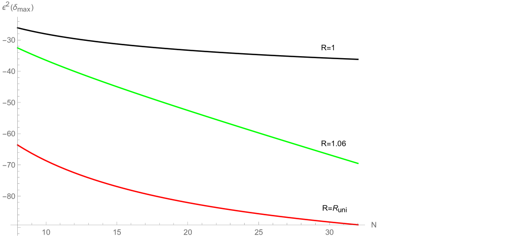
(b) Analytic Noise power bounds in dB with Conjecture (1) over various $N$ for different radii $R$.

Figure 13: Noise power bounds depending on radius $R$ and order $N$.

Proof.

Since the zeros are lying on two regular $N-$gons, and the nominator only needs one outer zero to be maximize, we can assume that the worst case scenario is given by Figure (15(b)). From (123) we obtain for the Huffman Zero Codebook

$$f^{2}(\mathscr{Z}) =\min_{\alpha\in\mathscr{Z}}|x_{N}(\alpha)|^{2}\min_{m\in[N]\setminus n}\min_{\theta}\frac{\prod_{n}|\alpha_{m}+\delta e^{i\theta}-\alpha_{m}|^{2}}{\sum_{n}|\alpha_{m}+\delta e^{i\theta}|^{2n}}$$ (140)

$$=\min_{\alpha\in\mathscr{Z}}|x_{N}(\alpha)|^{2}\min_{\theta}\frac{\prod_{n}|\alpha_{1}+\delta e^{i\theta}-\alpha_{m}|^{2}}{\sum_{n}|\alpha_{1}+\delta e^{i\theta}|^{2n}}.$$ (141)

Note, that $|x_{N}(\alpha)|$ is minimized by (27) if all zeros lie outside the unit circle, i.e.,

$$\min|x_{N}(\phi)|^{2}\geq\frac{R^{-2K}}{1+R^{-2K}}=\frac{1}{R^{2K}+1}.$$ (142)

Hence, by choosing $\theta=\pi$ and all zeros inside the unit disc except one, we get with (163) from Lemma (2)

$$f^{2}(\mathscr{Z}) \geq\frac{1}{R^{8M}+1}\frac{(R+\delta)^{2}-1}{(R+\delta)^{8M}-1}\cdot r^{4M-2}\delta^{4}(2a-\delta)^{4}\prod_{m=3}^{M}m^{4}\cdot$$ (143)

$$\quad\quad\left(\frac{\sin(2\pi/N)-\sin(4\pi/N)-2\sin(\pi/N)}{2(1-\sin(2\pi/N))}\right)^{4M-12}$$ (144)

∎

In Figure (13(a)) we plotted the exact bound (123) for Huffman Codebooks with optimal radius (102) for $N=4,8,16$ starting with the maximal radius $\delta_{max}={d_{\text{\rm min}}}/2$. It can be seen that for increasing $N$ the $\delta_{max}$ shifts to higher SNR, which indicates less noise robustness.

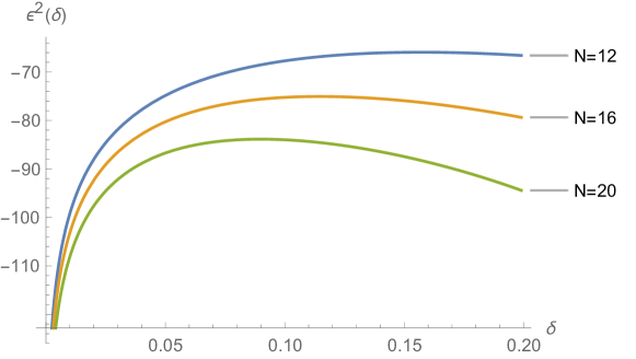
Figure 14: Analytic Noise power bounds (144) in dB for Huffman sequences with $R=1.02$ and various $N$.

XI Conclusion

We introduced a novel modulation scheme based on the zeros of the discrete-time signals to transmit reliable over unknown FIR channels. For the demodulation we presented three different approaches. The first based on a zero observation of the received zeros and deciding by a minimum distance decoder for each single bit (zero) independently. Secondly, a maximum likelihood decoder, which obtains the best performance. If the CIR length is larger than the block length, the ML decoder for Huffman BMOCZ outperforms all comparable known non-coherent signaling schemes. However, this decoder relies on the knowledge of the channels power delay profile and the SNR. Finally, we introduced a low-complexity decoder which decodes the zeros independently by only evaluating the received signal on the zero-codebook, which leads to linear complexity in the number of bits, instead of exponential complexity for the ML decoder. The derivation of bit error probabilities is mathematically hard to carry out, not only due to the overlap of the signals caused by multipath delays, but also in terms of the non-linear encoding in the zero domain. For the RFMD decoder we obtained a local stability analysis in the presence of additive noise, which suggest a proper zero separation of the codebook and channel. The analysis of reliable bit data rates and error probability bounds, based on a careful root neighborhood analysis, might be addressed in a future research.

XII Acknoledgements

The authors would like to thank Richard Kueng and Urbashi Mitra for many helpful discussions. We like to thank the SURF student Mattia Carrera for his support during a summer program at Caltech. Most of the work by Philipp Walk was done during a two year postdoc fellowship at Caltech, which was sponsored by the DFG WA 3390/1.

References

Appendix A Product distances from a circle point to the vertices of a regular polygon

We will adapt a result in [CK07b, Sec.5] to derive for any regular $N-$gon the extremal products of distances from a point on a circle centered at the centroid to all its vertices, see Figure (15(a)).

Theorem 4.

Let $N\geq 2$. Consider the regular $N-$gon inscribed in a circle of radius $r>0$ centered at the origin. The product of the distances to any fixed point $z=\delta e^{j\theta}$ on a circle of radius $0<\delta$ centered at the origin to the vertices is bounded by

$$|r^{N}+\delta^{N}|\geq g^{c}_{N}(z):=\prod_{n=1}^{N}d_{n}(z)\geq|r^{N}-\delta^{N}|.$$ (145)

The bounds are sharp and the extremal points are $z_{\text{min}}=\delta e^{jn\pi/N}$ resp. $z_{\text{max}}=\delta e^{jn2\pi/N}$, which lie on a line between one vertex and the origin respectively on a line between the middle point of two neighbor vertices and the origin. If the origin is added as an $N+1$ point the minimal and maximal product distance is achieved for the same $z_{\text{min}}$ and $z_{\text{max}}$ and given by

$$|r^{N}+\delta^{N}|\delta\geq\delta g^{c}_{N}(z):=\prod_{n=1}^{N+1}d_{n}(z)\geq\delta|r^{N}-\delta^{N}|.$$ (146)

(a) Points inside the polygon on a circle of radius $\delta$ (solid circle) resp. outside (dashed circle) with minimal (filled red) resp. maximal (non-filled ) distance products.

(b) Worst case constellation for Huffman polynomials.

Figure 15: Upper bounds for noise power which guarantee zero separation for $N=6$.

Proof.

Let us identify the vertices by complex numbers $r\omega^{m}$, where $\omega=e^{j2\pi/N}$ is the $N$th root of unity. Then the product of the distances from the vertices to any point $z$ is given by

$$g^{c}_{N}(z)=\prod_{m=1}^{N}d_{m}(z) =|z-r|\cdot|z-r\omega^{1}|\dots|z-r\omega^{N-1}|=|z^{N}-r^{N}|$$ (147)

Taking the product and inserting $z=\delta e^{i\theta}$ we get

$$g(\theta):=|\delta^{N}e^{Nj\theta}-r^{N}|^{2}=\delta^{2N}-2{\delta^{N}}r^{N}\cos(N\theta)+r^{2N}$$ (148)

We immediately find that $g$ is periodic in $[0,2\pi/N)$ and symmetric around $\theta_{c}=\pi/N$. Then, the critical points in the interval are given by the solutions of

$$0=g^{\prime}(\theta)=2N\delta^{N}r^{N}\sin(N\theta)\quad\Rightarrow\quad\theta_{1}=0,\ \theta_{2}=\pi/N.$$ (149)

Due to the symmetry of $g$ around $\theta_{1}$ and $\theta_{2}$, one of them must be a maximum and the other a minimum. Inserting both in (148) yields

$$g(0)=\delta^{2N}-2\delta^{N}r^{N}+r^{2N}=(r^{N}-\delta^{N})^{2}\quad,\quad g(\frac{\pi}{N})=(r^{N}+\delta^{N})^{2}$$ (150)

such that $g(0)$ is the minimum and $g(\pi/N)$ the maximum. Due to symmetry of the hexagon we can assume that the extremal point is in the gray area of Figure (15(a)). Hence, the minimal point lies on the real axis between the right vertex and the origin and the maximal point lies on the line crossing the midpoint of two vertices and the origin.

If we add the origin $0$ as the $N+1$ point, then $d_{N+1}=|0-z|=\delta$ for each $\theta$ and hence we only need to scale the upper and lower bounds by $\delta$. ∎

We will now ask for the case, where $z$ is placed on a circle with radius $\delta$ around one vertex, see the dashed circle in Figure (15(a)).

Conjecture 1.

Let $N\geq 2$ be an integer and $\omega=e^{j2\pi/N}$ be the $N$th root of unity. Then the points $r\omega^{n}$ are the vertices of a regular $N-$gon inscribed in the circle of radius $r>0$ centered at the origin. Let $0<\delta\leq r\sin(\pi/N)$ and consider any $z$ on a circle $C_{k}(\delta)$ of radius $\delta$ with center at one vertex $r\omega^{k}$, then the minimal product of all distances from $z$ to the vertices is given by

$$\min_{z\in C_{k}(\delta)}\prod_{n}|z-r\omega^{n}|=r^{N}-(r-\delta)^{N}.$$ (151)

Remark. If we add the origin of the $N-$gon as the $N+1$ point and demand $\delta<r\sin(\pi/N)$, then we get for the minimum of its product distances, by taking $k=0$

$$\prod_{n=1}^{N+1}d_{n}\geq\min d_{N+1}\cdot\min\prod_{n=1}^{6}d_{n}\geq(r-\delta)(r^{N}-(1-\delta)^{N})$$ (152)

since at any point $z=r+\delta e^{i\theta}$ the distance to the centroid is

$$d_{N+1}=|z-0|=|r+\delta e^{i\theta}|\geq|r-\delta|=r-\delta$$ (153)

where equality only holds for $\theta=\pi$, see Figure (15(a)). Note, $1-\sin(\pi/N)=\operatorname{versine}(\pi/2-\pi/N)=\operatorname{versine}((N-2)\pi/(2N))=2\sin^{2}((N-2)\pi/(4N))$ is monotone decreasing with increasing $N$. Hence $1-(1-\sin(\pi/N))^{N}$ will monotone increase with $N$. Moreover, for $N\geq 10$ we get

$$1-(1-\sin(\pi/N))^{N}\simeq 1$$ (154)

For $N=2$ the conjecture holds, since for $z=1+\delta e^{i\theta}$ we have

$$|1+\delta e^{i\theta}-1|\cdot|1+\delta e^{i\theta}+1|=\delta\cdot|2+\delta^{i\theta}|\geq\delta(2-\delta)=1-(1-2\delta+\delta^{2})=1-(1-\delta)^{2},$$

where equality holds if and only if $\theta=\pi$.

A-A Back to the Hexagon Lattice

If the Conjecture (1) would hold, we can similar argument as in (152), that if the origin is included as an $N+1$ point the minimum would be

$$\prod_{n=1}^{N+1}d_{n}(\theta)\geq(r-\delta)r^{N}(1-(1-\delta)^{N})$$ (155)

and be achieved for $\theta=\pi$. Furthermore, if we chose the circle around the centroid we get with Theorem (4)

$$|\delta|\prod_{n=1}^{N}|\delta e^{j\theta}-\alpha_{n}|\geq\delta(r^{N}-\delta^{N})$$ (156)

Indeed, we can then show, that the later product distance is the smallest possible.

Lemma 1.

Let $r>0$ and $N\geq 2$. Then it holds for any $\delta\in(0,r/2)$

$$\delta(r^{N}-\delta^{N})<(r^{N}-(r-\delta)^{N})\cdot(r-\delta).$$ (157)

Proof.

To show this, we only need to verify for $r=1$ and $\delta\in(0,1/2)$, i.e.,

$$\delta(1-\delta^{N}) <(1-(1-\delta)^{N})(1-\delta)$$ (158)

$$\Leftrightarrow\quad a_{N}=\delta-\delta^{N+1} <(1-\delta)-(1-\delta)^{N+1}=b_{N}$$ (159)

For $\delta=1/2$ and $\delta=0$ this becomes equality. We will prove the strict inequality by induction. For $N\geq 2$ we get

$$b_{2}=1-\delta-(1-3\delta+3\delta^{2}-\delta^{3})=2\delta-3\delta^{2}+\delta^{3}=b_{2}+\delta+2\delta^{3}-3\delta^{2}$$ (160)

But for the last three terms it holds

$$\delta+2\delta^{3}-3\delta^{2}>0\quad\Leftrightarrow\quad 1+2\delta^{2}>3\delta\quad\Leftrightarrow\quad\delta^{-1}+2\delta>2+1=3.$$ (161)

Note, for $N=1$ the strict inequality (159) does not hold, since $\delta(1-\delta)=(1-1+\delta)(1-\delta)$. We will now show that (159) holds for $N+1$. From (159) we get

$$a_{N+1} =\delta-\delta^{N+2}=\delta(\delta-\delta^{N+1})-\delta^{2}+\delta=\delta a_{N}+(1-\delta)-(1-\delta)^{2}$$

$$b_{N+1} =(1-\delta)-(1-\delta)^{N+2}=(1-\delta)b_{N}+(1-\delta)-(1-\delta)^{2}>\delta b_{N}+(1-\delta)-(1-\delta)^{2}$$

where we used $1-\delta>\delta$ for each $0\leq\delta<1/2$. Hence it holds $b_{N+1}>a_{N+1}$ if $b_{N}>a_{N}$ holds. By induction and (160) this holds for all $N\geq 2$. ∎

The lower bound (157) is monotone increasing for $\delta\in[0,r/2]$ and achieves its maximum at the boundary $\delta=r/2$ given by

$$0\leq\delta(r^{N}-\delta^{N})\leq\frac{r^{N+1}}{2}\frac{(2^{N}-1)}{2^{N}}<\frac{r^{N+1}}{2}$$ (162)

see Figure (17(b)) for the hexagon, $N=6$ and $r=1$.

Figure 16: Lower bound conjecture for regular $N-$gon with circle point around one vertex.

We will now lower bound the product distances in Conjecture (1) for $N-$gons with circle points around one vertex, by using the geometric relaxation given in Figure (16).

Lemma 2.

Consider a regular $N-$gon with $N=4M$ for any $3\leq M\in{\mathbb{N}}$ inscribed in a circle of radius $r>0$. Consider a point $z$ on a circle with radius $\delta<r\sin(\pi/N)$ and center $z=r+\delta e^{i\theta}$. Then the minimal product distances for all $\theta$ is bounded by

$$g_{v,N}(\theta)\geq\prod_{n}d_{n}\geq\delta(2r-\delta)\prod_{m=1}^{M}(1+\sin\frac{\pi}{2M}-2\tilde{\delta}(\tilde{\delta}+1+\sin\frac{\pi}{2M}))\cdot r^{4}\sin^{2}\frac{\pi}{4M}(\prod_{m}2m-1)^{2}$$ (163)

Proof.

Lets define $\omega=e^{j2\pi/N}$. We will use two reference points, at $r-2\delta$ and at $r$, to lower bound the distances to the vertices. The special distance

$$d_{2M+1}=|\alpha_{2M+1}-z|\geq 2r-\delta\quad,\quad d_{1}=\delta$$ (164)

For all vertices in the left half plane we will use the radius of the smallest circle given by

$$b_{M+2}=\sqrt{(r+c-\sqrt{2}\delta)^{2}+(r-h)^{2}}$$ (165)

where

$$c=r\sin(\gamma)=r\sin(\pi/2M)\quad,\quad h=r(1-\cos(\gamma)),\quad,\quad a=2r\sin(\pi/4M).$$ (166)

which gives

$$b_{M+2} =\sqrt{r^{2}(1+\sin(\pi/2M)-2\tilde{\delta})^{2}+r^{2}(1-(1-\cos(\pi/2M)))^{2}}$$ (167)

$$=r\sqrt{2}\sqrt{(1+\sin(\pi/2M)+\tilde{\delta}^{2}-\sqrt{2}\tilde{\delta}(1+\sin(\pi/2M))}$$ (168)

The distances in the first quadrant we will lower bound by multiples of $\frac{b_{2}}{2}$ given as

$$\frac{b_{2}}{2}=a\cdot\cos(\pi/4)/2=2r\sin(\pi/4M)\frac{\sqrt{2}}{4}=r\sin(\pi/4M)\frac{1}{\sqrt{2}}$$ (169)

Then we get for the product of all distances the bound

$$g_{v,4M} =\prod_{n}d_{n}\geq b_{M+2}^{2M-2}\cdot d_{1}\cdot d_{2M+1}\cdot\prod_{m=1}^{M}((2m-1)\frac{b_{2}}{2})^{2}$$ (170)

$$=\delta(2r-\delta)\prod_{m=1}^{M}2r^{2}(1+\sin(\pi/2M)-2\tilde{\delta}(\tilde{\delta}+1+\sin(\pi/2M)))\cdot(2m-1)^{2}\frac{r^{2}\sin^{2}(\pi/4M)}{2}$$

$$=\delta(2r-\delta)\prod_{m=1}^{M}(1+\sin\frac{\pi}{2M}-2\tilde{\delta}(\tilde{\delta}+1+\sin\frac{\pi}{2M}))\cdot r^{4}\sin^{2}\frac{\pi}{4M}(\prod_{m}2m-1)^{2}$$ (171)

∎

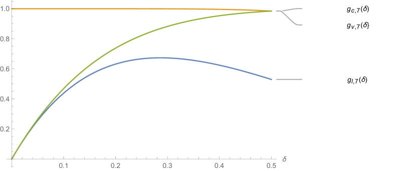
(a) Bounds for $r=1$ without centroid.

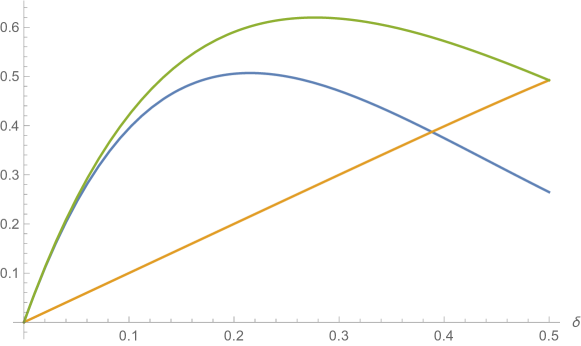
(b) Bounds with centroid.

Figure 17: Lower Bound for Hexagon Conjecture (green line). Yellow line for bound the $g_{c}$ at centroid circle.