On definite lattices bounded by a homology 3-sphere
and Yang-Mills instanton Floer theory
Abstract
Using instanton Floer theory, extending methods due to Frøyshov, we determine the definite lattices that arise from smooth 4-manifolds bounded by certain homology 3-spheres. For example, we show that for +1 surgery on the (2,5) torus knot, the only non-diagonal lattices that can occur are and the indecomposable unimodular definite lattice of rank 12, up to diagonal summands. We require that our 4-manifolds have no 2-torsion in their homology.
1 Introduction
Let be a smooth, closed and oriented 4-manifold. The intersection of 2-cycles defines the structure of a unimodular lattice on the free abelian group . Donaldson’s celebrated Theorem A of [Don86] says that if this lattice is definite, then it is equivalent over the integers to a diagonal form . Donaldson’s original proof used instanton gauge theory, and alternative proofs were later given using Seiberg-Witten and Heegaard Floer theory [OS03, Thm.9.1], in conjunction with a lattice-theoretic result due to Elkies [Elk95a].
For a given integer homology 3-sphere , which definite lattices arise as the intersection forms of smooth 4-manifolds with boundary ? Donaldson’s theorem may be viewed as the solution to this problem in the case of the 3-sphere. To date, there is only one result in which the set of definite lattices is determined and does not consist of only diagonal lattices: under the assumption that the 4-manifolds are simply-connected, Frøyshov showed in his PhD thesis [Frøb] that the only non-diagonalizable definite lattices bounded by the Poincaré sphere are . The proof uses instanton gauge theory, and no other proofs are yet available.
In this article we extend and reformulate some of Frøyshov’s methods in [Frøb, Frø04] to obtain further results in this direction. The central new application is the following.
Theorem 1.1.
Let be an integer homology 3-sphere -homology cobordant to surgery on a knot with smooth 4-ball genus 2. If a smooth, compact, oriented and definite 4-manifold with no 2-torsion in its homology has boundary , then its intersection form is equivalent to one of
where is the unique indecomposable unimodular positive definite lattice of rank 12.
If a non-diagonal lattice in this list occurs, then for does not: if the former arises from and the latter from , both with boundary , then the closed 4-manifold has a non-diagonal form, contradicting Donaldson’s Theorem A. An example realizing all the positive forms on the list is surgery on the torus knot, which is the Brieskorn sphere .
Corollary 1.2.
If a smooth, compact, oriented and definite 4-manifold with no 2-torsion in its homology has boundary , then its intersection form is equivalent to one of
and all of these possibilities occur.
The realizations of these lattices are straightforward, except perhaps for the case of ; see e.g. [GS18]. A slightly more general statement of Theorem 1.1 follows from Corollary 4.3 below. Theorem 1.1 may be viewed as the next installment of the following, which itself is a kind of successor to Donaldson’s Theorem A cited above.
Theorem 1.3.
Let be an integer homology 3-sphere -homology cobordant to surgery on a knot with smooth 4-ball genus 1. If a smooth, compact, oriented and definite 4-manifold with no 2-torsion in its homology has boundary , then its intersection form is equivalent to one of
A corollary is a slight improvement of Frøyshov’s theorem, obtained by applying the result to surgery on the torus knot, the orientation-reversal of the Poincaré sphere :
Corollary 1.4 (cf. [Frøb]).
If a smooth, compact, oriented and definite 4-manifold with no 2-torsion in its homology has boundary , then its intersection form is equivalent to one of
and all of these possiblities occur.
We give more examples in Section 5. We expect the methods used to provide further applications. A good candidate to consider next is , which is surgery on the torus knot of genus 3. In [GS18] we show that this manifold bounds the unimodular lattices , , , and , the last two being the indecomposable positive definite unimodular lattices of ranks 14 and 15, respectively; we exhibit some of these in Section 5.
A straightforward Mayer-Vietoris argument shows that the statements of both Theorems 1.1 and 1.3 hold for 3-manifolds that are not integer homology 3-spheres, as long as the lattice is assumed to be unimodular. In joint work with Marco Golla [GS18] we provide analogues of the above results for non-unimodular lattices.
Other than Donaldson’s Theorem A and Frøyshov’s work in instanton Floer theory, restrictions on the possible definite lattices bounded by a fixed homology 3-sphere have previously been established using Seiberg-Witten and Heegaard Floer theory. In particular, there is a fundamental inequality for both the Heegaard Floer -invariant of Oszváth and Szabó [OS03, Thm.1.11] and Frøyshov’s Seiberg-Witten correction term [Frø10, Thm.4]. A lattice theoretic result of Elkies [Elk95b] implies that if an integer homology 3-sphere has either of these invariants the same as that of the Poincaré sphere, then there are only 14 possible definite lattices that occur, up to diagonal summands; see Table 1. While our proofs of all results stated above depend only on instanton theory, we will see in Section 3.2 that for Theorem 1.3 these restrictions from other theories can replace some, but not all, of the instanton theoretic input of the argument. The same is true for Theorem 1.1, as discussed at the end of Section 4.
To prove Theorems 1.1 and 1.3, we provide partial analogues of Frøyshov’s instanton inequality from [Frø04] in which the coefficients used are the integers modulo two and four. The inequalities provide new lower bounds for the genus of an embedded surface in a smooth closed 4-manifold in terms of data from the intersection form. Part of the input for these inequalities are relations in the instanton Floer cohomology ring of a circle times a surface, taken with the coefficient rings and . We only prove the relevant relations for low genus, which is more than what is needed for our applications. We also reduce the verification of the general case to an arithmetic problem that we plan to return to in a separate article.
Apart from the determination of the relations just mentioned, the proofs of the inequalities we use are straightforward adaptations of the characteristic zero case from [Frø04], as explained in Section 7. Alongside our and adaptations we also digress in Section 7.3 to discuss analogues of Frøyshov’s inequality for odd characteristic coefficients. The reader should also have no trouble formulating adaptations for coefficients where . However, these other variations are not utilized for any applications in this article.
Frøyshov has announced in several public lectures over the years the construction of two homology cobordism invariants, denoted and , defined using the second and third Stiefel-Whitney classes of the basepoint fibration in the context of mod two instanton Floer theory, in a fashion similar to his construction of the -invariant of [Frø02]. We expect the mod two inequality, Theorem 2.1 below, to be completed to one which allows the 4-manifold to have homology 3-sphere boundary, by perhaps involving the invariant , in analogy with Frøyshov’s inequality of [Frø04]. Similarly, the homology cobordism framework of [Frø02] might be adapted to enrich the mod four inequality, Theorem 2.2 below. We rather indirectly touch upon these matters in Section 8, where we replace our first arguments with some using instanton Floer theory for homology 3-spheres.
Outline. In Section 2 we state the inequalities obtained from instanton theory, our main technical tools. The proofs of these, which are adaptations of Frøyshov’s argument to the settings of and coefficients, are presented in Section 7. In Section 3 we prove Theorem 1.3 and Corollary 1.4. In Section 4 we prove Theorem 1.1 and Corollary 4.3. More examples are presented in Section 5. In Section 6 we prove some relations in the instanton cohomology of a circle times a surface. An alternative proof of Corollary 1.2, closer in spirit to Frøyshov’s proof of Corollary 1.4 and emphasizing the role of instanton Floer homology for homology 3-spheres, is presented in Section 8. Finally, in Section 9, we discuss an example of a rank 14 definite unimodular lattice which illustrates the necessity of the mod 4 data used in the proof of Theorem 1.1.
Acknowledgments. The author thanks Kim Frøyshov for his encouragement and several informative discussions. The work here owes a great debt to his foundational work in instanton homology. Thanks to Motoo Tange for being the first to inform the author that bounds . The author also thanks Marco Golla, Ciprian Manolescu, Matt Stoffregen and Josh Greene for helpful correspondences. The author was supported by NSF grant DMS-1503100.
2 The inequalities
In this section we state partial analogues of Frøyshov’s instanton inequality from [Frø04] when the coefficients used are the integers modulo two and four. The proofs are presented in Section 7. In addition, for context, we recall Frøyshov’s inequality of [Frø04]. The reader interested in the applications may wish to skip this section and refer back when needed.
Let denote the -graded instanton cohomology of a circle times a surface of genus equipped with a -bundle having odd determinant line bundle. The 4D cobordism defined by a 2D pair of pants cobordism crossed with the surface induces a map endowing with the structure of an associative ring with unit. Muñoz [Mn99] determined a presentation for this ring over which is recursive in the genus, and we will see later that is torsion-free. There are two distinguished elements in , denoted and , of degrees and mod 4, respectively. Define
for , and . Here denotes the quotient of by relative Donaldson invariants involving -classes of loops; see Sections 6 and 7.2 for more details. The element (mod 2) in may be defined using the second Stiefel-Whitney class of the basepoint fibration.
Now we state the inequality that comes from working with mod two coefficients. Given a definite lattice we define a non-negative integer as follows. For a subset denote by the elements which have minimal absolute norm among elements in . Note is of even cardinality when it is not , since then acts freely on it. We call extremal if it is of minimal absolute norm in its index two coset, i.e. . If , set . Otherwise,
| (1) |
Theorem 2.1.
Let X be a smooth, closed, oriented 4-manifold with no 2-torsion in its homology. Suppose . Let for be smooth, orientable and connected surfaces in of genus with self-intersection 1 which are pairwise disjoint. Denote by the unimodular negative definite lattice of vectors vanishing on the classes . Then we have
| (2) |
where is a non-negative integer invariant of the unimodular lattice defined below in (4), which satisfies , and vanishes if and only if is diagonalizable.
As mentioned in the introduction, the proof is an adaptation of the characteristic zero case in [Frø04]. Rather than cutting down moduli spaces of instantons using the first Pontryagin class of the basepoint fibration, we use the second Stiefel-Whitney class. If we define and
for then the same technique is applied to the situation of mod 4 coefficients. In this case we cut down moduli spaces using the first Pontryagin class of the basepoint fibration, which in corresponds to the element , and we obtain the following inequality.
Theorem 2.2.
Let X be a smooth, closed, oriented 4-manifold with . Let for be smooth, orientable and connected surfaces in of genus with self-intersection 1 which are pairwise disjoint. Let denote the torsion subgroup. Let be the unimodular negative definite lattice of vectors vanishing on the classes . If is odd then
| (3) |
where is a non-negative integer invariant of the unimodular lattice defined below in (6), which satisfies , and vanishes if and only if is diagonalizable. If is twice an odd number, then the same inequality holds upon replacing with .
If is negative definite, all inequalities above apply to with the genus zero exceptional sphere; in this case, is the lattice of . The vanishing of the left side of either inequality forces to be diagonal, implying Donaldson’s diagonalization theorem [Don86] under some hypothesis on the 2-torsion of . In fact, the term , which also vanishes if and only if is diagonal (see Prop. 2.4), essentially appears in Fintushel and Stern’s proof of Donaldson’s theorem [FS88].
The effectiveness of the inequalities towards our applications comes from the determination of and . In Section 6 we give evidence that the relations (mod 2) and (mod 4) hold in for all . For our applications, we only need verify this for . To this end:
Proposition 2.3.
For we have and .
We will in fact reduce the verification of this proposition for general to an elementary arithmetic problem which we do not attempt to solve in this article. The threshold is insignificant, and is the extent to which we have verified the formulas with a computer. We now proceed to define the lattice terms and appearing in Theorems 2.1 and 2.2.
Let be a definite unimodular lattice. Given write for their inner product, and for . For write for the sublattice of elements satisfying (mod 2). Given , define a linear form by first letting where each , and then extending linearly over . Next, define
| (4) |
where the maximum is over triples where is nonzero and extremal, , , and, as indicated in (4) above, (mod 2), where
| (5) |
In (4) we use the convention that . The conditions and imply that is an integer divisible by . The signs appearing in do not actually matter for the definition of , but do matter for the definitions to follow. When we interpret ; in this case we simply write . Note that when is an even lattice the signs appearing in are all positive. We remark that our definition of is essentially that of [Frø02] and one half of that in [Frø04], except that in those references, only is used. Note that (mod 2) is equivalent to the condition that (mod 2), and thus . We do not have an example for which , but we include in the statement of Theorem 2.1 because it arises naturally in the proof. However, for all of our applications that use Theorem 2.1 we will only bound from below.
Moving on to the lattice term in the mod 4 setting, we define
| (6) |
where the maximum is over triples where is nonzero and extremal, with (mod 2), with , and (mod 4), as is indicated in (6). As claimed in Theorem 2.2, we have the following:
This follows directly from the definitions if for an extremal vector with and (mod 2) where is even. If instead is odd, we use that (mod 2), which holds since all vectors in have the same mod 2 inner product with .
Proposition 2.4.
Each of , and vanish if and only if is diagonalizable.
Proof.
Assume for simplicity that is positive definite, and write where contains no vectors of square . If is non-diagonalizable, then . Let be of minimal nonzero norm in . Suppose and . Without loss of generality suppose . Then . On the other hand, , and so since is minimal in . We obtain . We conclude that and , and thus . The converse may be proved by direct computation, or we can apply Theorems 2.1 and 2.2 with and the exceptional sphere in to obtain that for the diagonal lattice . ∎
These lattice terms should be compared to the analogous term appearing in Frøyshov’s inequality for the instanton -invariant, which we now recall. In fact, we will state a slightly more general result. We define for a definite unimodular lattice the following quantity:
| (7) |
where the maximum is over triples where is extremal, , (mod 2), , and , as is abbreviated in (7). From the definitions we have
Denote by Frøyshov’s instanton -invariant defined in [Frø02]. We next define
for and . The computation due to Muñoz [Mn99, Prop.20] is used in Frøyshov’s inequality, and determines the left hand sum in the following.
Theorem 2.5 (cf. [Frø04] Thm.2).
Let X be a smooth, compact, oriented 4-manifold with homology 3-sphere boundary and . Let for be smooth, orientable, connected surfaces in of genus with which are pairwise disjoint. Denote by the unimodular lattice of vectors vanishing on the classes . Then
| (8) |
We have lifted the restriction in [Frø04] that all but one of the surfaces have genus 1. This follows from a minor technical improvement of the proof, which uses the existence of a perfect Morse function on the moduli space of projectively flat connections on a surface with fixed odd determinant. This is explained in Section 7.
Each of the lattice terms defined above arises from adapting the proof of Frøyshov’s inequality; each such adaptation has a choice of coefficient ring, a corresponding relation in the instanton cohomology ring of a circle times a surface, and a possible assumption on the torsion group of the 4-manifold. We summarize the expected scheme for all cases considered above as follows:
| Lattice term | Coefficients | Relation | Torsion assumption |
|---|---|---|---|
| none | |||
| (mod 2) | |||
| (mod 4) | |||
| (mod 4) |
The relations are to be understood within , although we expect the mod 2 and mod 4 relations, which as listed are only verified for in this paper, to hold in . The first row corresponds to Theorem 2.5, the second row to Theorem 2.1, and the third and fourth rows to Theorem 2.2.
We have only included in our discussion the variations of Frøyshov’s inequality we have found useful for our applications. However, the proof of Theorem 2.5 is easily adapted to any coefficient ring. We discuss this to some extent in Section 7.3.
We will not use the inequality of Theorem 2.2 with equal to twice an odd number, corresponding to the last row in the above table. In the absence of 2-torsion, this inequality is in fact implied by that of Theorem 2.1. However, since the torsion hypothesis in the former inequality is weaker than that of the latter, the two inequalities provide different information.
In Section 9 we will show that the indecomposable unimodular postive definite lattice of rank 14 has , while and . This example shows that Theorems 2.1 and 2.5 cannot alone prove Theorem 1.1. We will show, on the other hand, that Theorem 1.3 can be proven with Theorem 2.1 and some input from Seiberg-Witten or Heegaard Floer theory.
3 Genus 1 applications
In this section we prove Theorem 1.3 and Corollary 1.4 assuming the inequalities of Theorems 2.1 and 2.2. We then give another proof of Theorem 1.3 using the Heegaard Floer -invariant and only Theorem 2.1. We begin with a corollary of our main inequalities that follows [Frø04, Cor. 1].
For a link in an integer homology 3-sphere , we define to be the minimum over all such that there exists a -homology 4-ball with and an oriented, genus surface smoothly embedded in with and an isomorphism. If no such data exists, we set . If is a knot in the 3-sphere, note that , the latter quantity being the smooth 4-ball genus of .
Corollary 3.1.
Let be the result of performing -surgery on each component of a link in an integer homology 3-sphere. If bounds a smooth, compact, oriented 4-manifold with no 2-torsion in its homology and negative definite intersection form , then for we have
To obtain the corollary, let be the orientation reversal of the negative definite surgery cobordism from to . Then apply Theorems 2.1 and 2.2 to the closed 4-manifold , which has , and contains disjoint surfaces of self-intersection formed by capping off the components of a surface bounded by as above with disks from the 2-handles of the surgery cobordism . Proposition 2.3 determines the left hand sides of (2) and (3) for , and the corollary follows. A similar corollary can be obtained by slightly weakening the 2-torsion assumption on and using only , but we will not need this variation; however, see Remark 3.5.
3.1 The proof of Theorem 1.3 using Theorems 2.1 and 2.2
We recall some basic notions from the theory of lattices. Let us call a definite lattice reduced if there are no elements of squared norm . A root in a reduced definite lattice is an element with square . A root lattice is a reduced positive definite lattice generated by its roots. Examples are and , each associated to a Dynkin diagram:
The root lattice is obtained by taking as basis the vertices, each having square ; if two vertices are joined by an edge, their inner product is , and is otherwise . For we require , and for , . In each case, is the number of vertices, or the rank of the lattice. It is well-known that any positive definite root lattice can be written as a direct sum of these given lattices.
To simplify the notation below, we assume henceforth that is a positive definite unimodular lattice. Any such lattice can be written as where is reduced and . We write for the root lattice generated by the roots of , and also call the root lattice of . In general, is not determined by , but it is common in many cases to notate by the data , cf. [CS99, Ch.16]. For example, we write for the rank 15 unimodular positive definite lattice whose root lattice is isomorphic to . For this reason we have used different fonts for unimodular lattices and root lattices, although . The presence of an “” indicates an empty root lattice; for example, the lattice , called the shorter Leech lattice, has no roots.
Lemma 3.2.
If then the root lattice is indecomposable.
Proof.
Write as above, so that . Suppose is extremal in and . We first claim that . Let with , and suppose without loss of generality that . Then . On the other hand, implies , since has vectors only of square . We conclude , contradicting the assumption that is extremal. This proves the claim.
Now suppose that is decomposable. Then there are both of square and . Set , which has . Then contains 4 elements, and (mod 4). Thus . ∎
Lemma 3.3.
If and is indecomposable, then for some .
Proof.
We claim the map induced by inclusion is an isomorphism. (This is essentially the proof of [Frøb, Lemma 4.3].) Suppose it is not. Choose of minimal norm such that is not in the image of . In particular, is extremal. Now suppose is extremal with and . If then , the last inequality by minimality of . This is a contradiction, and so . In particular, . Then implies . But implies , whence . It follows that . Then , since is not a root, contradicting our hypothesis on .
Thus is an isomorphism. In particular, and is odd. If is indecomposable, the latter condition implies that is either zero, , or for even. That when follows from direct computation, or by applying Corollary 3.1 to surgery on the torus knot, which bounds .
If is zero, so is , since the ranks are equal. But then is diagonal, contradicting . Next, suppose . A standard model of is the sublattice of spanned by vectors whose coordinates add up to zero. Suppose , and let . Then is extremal in with square 4, and consists of the vectors obtained from by permuting the two signs. Thus , implying . Finally, the cases and are ruled out by ; it is well-known that there are no unimodular, non-diagonal definite lattices of rank . ∎
The only non-diagonal lattices that occur under the hypotheses of both lemmas above are those with reduced part . From Corollary 3.1 we obtain the following, which, along with the observation that the statement is -homology cobordism invariant (see Section 5), implies Theorem 1.3.
Corollary 3.4.
Let be the result of surgery on the components of a link in a homology 3-sphere with . If is a smooth, compact, oriented and definite 4-manifold bounded by with non-diagonal lattice and no 2-torsion in its homology, then for some .
Proof of Corollary 1.4.
The manifold is surgery on the torus knot of genus 1. By Theorem 1.3 it remains to realize the listed lattices. The corresponding surgery cobordism provides the form , and bounds a plumbed manifold with lattice . After connect summing with copies of we obtain from these and for . Finally, cannot occur; for if it did, gluing the orientation reversed 4-manifold to the plumbing would yield a non-diagonal definite lattice , contradicting Donaldson’s diagonalization theorem. ∎
As mentioned in the introduction, Corollary 1.4 is a slight improvement on the main result of Frøyshov’s PhD thesis [Frøb]. The proof is much the same as far as the lattice theoretic input is concerned, and has only been repackaged and presented differently. We next prove the same result in a different way, making use of some input from Heegaard Floer theory.
3.2 The proof of Theorem 1.3 using Theorem 2.1 and the -invariant
The fundamental inequality for the Heegaard Floer -invariant of Oszváth and Szabó [OS03, Thm. 1.11] states that if is an integer homology 3-sphere, and is a smooth, negative definite 4-manifold bounded by , then for any characteristic vector , we have
| (9) |
Recall that a characteristic vector is an element that satisfies (mod 2) for every in the lattice. It is classically known that the square of any characteristic vector is modulo 8 the rank of the lattice. Elkies showed in [Elk95b] that, up to adding diagonal summands , there are a finite number of positive definite unimodular lattices with no characteristic vectors of squared norm less than , where is the rank of the lattice. There are in fact 14:
| 8 | 12 | 14 | 15 | 16 | 17 | 18 | 19 | 20 | 21 | 22 | 23 | |
|---|---|---|---|---|---|---|---|---|---|---|---|---|
| , | , |
Thus by (9), if a non-diagonal definite lattice is bounded by with , as is the case for the orientation-reversal of the Poincaré homology 3-sphere, it must be one of these 14 lattices, possibly upon adding . We remark that Seiberg-Witten theory can also be used make this reduction, as Frøyshov’s monopole invariant (rescaled) also satisfies (9), see [Frø10, Thm. 4]. It is known that if is -surgery on a knot of slice genus 1 we have , see (24). According to Elkies [Elk95a], if , the only possible definite lattices that can bound are diagonal.
With this input, the proof of Theorem 1.3 follows using only the inequality in Corollary 3.1 that comes from Theorem 2.1. It suffices to show that for all lattices on Elkies’ list which are not . This follows from the fact that the lattices on the list other than have a vector of square 3. In fact, if is the number of vectors of squared norm in a lattice of rank in Table 1, then , and , see [Elk95b, Thm. 1] and also [NV03, eq. U3]. Using the by now familiar argument, for any with we have , whence , completing our second proof of Theorem 1.3.
4 Genus 2 applications
In this section we prove Theorem 1.1. We continue our notation of lattices from Section 3. We begin with a family of examples for later reference. Using the notation of [Frø04] we set
| (10) |
where . We remark that is diagonalizable, and . The lattice is even precisely when is even. We note that is the same as from Table 1, the latter notation indicating that the root lattice of is . The lattice is isomorphic to the intersection form of the positive definite plumbing with boundary the orientation-reversed Brieskorn sphere :
Via (10), the node corresponds to the vector , while the other nodes correspond to and . Replacing by in this collection yields the root lattice .
Proposition 4.1.
and .
Proof.
It is shown in [FS01, §2] that can be decomposed as , where is the negative definite plumbing of with intersection form and is obtained from attaching to the 4-ball a -framed 2-handle along the torus knot and a -framed 2-handle along a meridian of the torus knot. Blowing down the meridian 2-handle yields such that , with a decomposition where is obtained by attaching only a -framed 2-handle to the torus knot. Since the torus knot has genus , the 2-handle can be capped off to form a surface of genus . The lattice of vectors vanishing on is isomorphic to .
This should be compared to [Frø04, Prop.1]. There it is shown that . Thus the family of 4-manifolds with surface just given achieve sharpness in Frøyshov’s inequality of Theorem 2.5. Proposition 2.3 shows that the same family achieves sharpness in the inequalities of Theorems 2.1 and 2.2 for low , and we expect this to be true for all . We remark that the same 4-manifolds are used by Behrens and Golla [BG] in the Heegaard Floer context.
We now move on to the main line of argument for Theorem 1.1. Recall that for the proof of Theorem 1.3, we used Lemma 3.2, which says implies the root lattice of is indecomposable. The key algebraic input towards the proof of Theorem 1.1 is the following upgrade.
Lemma 4.2.
If then is one of or .
Proof.
From Lemma 3.2 we know is indecomposable, and hence one of or zero. We will again use that with has , as shown in the proof of Lemma 3.2. All extremal vectors chosen below have the property that the elements in have the same signs in the expression for when .
Suppose . A standard model for is the sublattice of consisting of vectors whose coordinates add to zero. Let . Then is extremal in of square 4, and consists of the 12 vectors obtained by permuting the signs of and those of . Thus (mod 4), and .
Suppose . A standard model for is the sublattice of consisting of vectors whose last three coordinates are equal. Consider , extremal and of square 4. Then consists of the 8 vectors with an even number of signs, as well as the 2 vectors . Thus (mod 4), and .
Suppose , . As in the proof of Lemma 3.3, take , for which has 6 extremal vectors. Then (mod 4), and .
Suppose . Let be the map induced by inclusion. This map cannot be onto, since any unimodular lattice of rank is diagonal. Choose of minimal norm such that . We showed in the proof of Lemma 3.3 that . Since , . If then . So suppose . Further suppose . Then is extremal of square 5 and . We compute . It follows that . Now instead suppose is not orthogonal to . From and the assumption that has no vectors of square we obtain for each root . Let be roots satisfying , so that is the set of all roots. The condition implies, after possibly relabeling, that , and . Then is an extremal vector of square 5, , and , again implying .
Suppose . Again, is not onto, and its cokernel has rank at least 2, since no unimodular lattice of rank has root lattice . Again choose of minimal norm such that . If , we are done; so suppose . Let be the unique root in up to sign. If , then as in the case for we can use to conclude . So assume . As before, , so in fact . Let be of minimal norm such that . Then the same argument as in the proof of Lemma 3.3 shows . If , we are done; so suppose . If , then take as in the case of . Suppose instead . As with , we have , so . Since , by minimality of we have , from which it follows that . If , then for some choice of signs, has square 4; if , then one of has square 4. In either case we obtain a vector of square 4, and take this as our extremal vector to obtain .
Next, suppose for some . Suppose has full rank within , i.e. the map induced by inclusion is an isomorphism. The only full rank embeddings of into a non-diagonal unimodular lattice are those inside with (see e.g. [Ebe13, Sec.1.4]), and we have computed . If then either , in which case , contradicting the assumption that , or , in which case . Thus we may assume that is not onto. It follows also that is not onto, since . We will see that the arguments below generalize those for the cases of and given above.
We begin as in the case for . Let be of minimal norm such that . If we are done, as argued in the above cases, and so we may assume . We may also assume . Indeed, consider the map . The codomain here is a free abelian group of rank equal to . The argument in Lemma 3.3 shows that for a given proper subspace , any of minimal norm among vectors such that has ; in Lemma 3.3, . In particular, we may choose to be the kernel of . By construction, .
Choose a root such that , following the argument as in the case of . Then is extremal of square . Let . Assume and . Write where . Then implies is a root. Recall for any root that from we have , and if . Then
implies either or . Let be the set of roots such that . We conclude . Let . We compute
| (11) |
If we set , using , and the definition of , from (11) we compute
| (12) |
If (12) is nonzero modulo 4, then and we are done. So henceforth assume (mod 4).
We represent as the sublattice of of vectors whose coordinates sum to zero. Henceforth we identify the vectors in this representation of with those in the root lattice of . We may suppose that , since the automorphism group of acts transitively on roots. Here we write for the standard basis vectors of . Then the vectors
| (13) |
make up the set of roots such that . For a fixed we have the two relations
| (14) | ||||
| (15) |
Pairing (14) with , we see that either , or . Similarly for (15). Thus has , or elements. Furthermore, .
Now let with even. Then there exists such that
| (16) |
To see this, let be the vector corresponding to which has if and otherwise, and then compute (16) using (11). From (16) we may assume that either (I) for all or (II) for all . Indeed, if and for some then setting in (16) yields (mod 4).
Case (I). Suppose for all . Then . Having assumed (mod 4), we conclude (mod 4). Set . Since , and implies one of or is orthogonal to and the other has inner product with , we obtain . In a similar fashion, for each let be such that and . For set . This is a vector in whose and entries are , with all other coordinates zero. Then are orthogonal roots all satisfying . Since , its length is strictly greater than that of its projection onto the span of the subspace in generated by the :
| (17) |
Recalling and (mod 4), we must have , i.e. . Before considering these two cases separately, we determine one more constraint. Suppose and for some ; the superscripts here are not important. Then is a root for which , a contradiction. Thus for each , for some uniform , and each . We conclude that after perhaps reflecting some coordinates in the range and permuting the first two coordinates in our representation of we have .
Now suppose . Setting , we choose of minimal norm such that . We may suppose each , or else we are done. Our previous arguments show for and for all roots . We only need to do this for , which is possible because there are no definite unimodular lattices of rank with root lattice ; the first non-diagonal definite unimodular lattice, by rank, is . By our assumption from the previous paragraph, . Define the dual lattice , and let
denote projection. The values for all roots are determined and given by column (i) in Table 2, which lists one root for each pair . In particular, we see that . Note is orthogonal to exactly half the roots in . We may also assume case (I) for and , each with respect to some orthogonal root. Then, just as was established for , each of is orthogonal to half the roots of . Thus two of are orthogonal to a common root. Without loss of generality, suppose these two vectors are and , and that the orthogonal root is . Recalling (mod 4), formula (11) yields
| (18) |
Thus we may assume that is either orthogonal to or pairs non-trivially to with both of its vectors. Combining this with the constraints for previously determined for , the pairings of with the roots of must be given by one of columns (i)-(iv) in Table (2). In particular, or . The case of will now be completed by constructing an extremal vector of square 4 such that (mod 4), following the cases of and above. There are two cases to consider: and .
| (i) | (ii) | (iii) | (iv) | |
|---|---|---|---|---|
First, suppose . Upon possibly replacing with , the pairings of with are given by either (i) or (iii) in Table 2. Then is of square , where . As usual, if is extremal, then is a root, and the condition implies , and thus
| (19) |
Now each of has for any root , and so in (19) must be orthogonal to one of the three, and have pairing with the other two. If has pairings given by (i) in Table 2, then the set of such is given by . Thus has 2 elements, implying . If instead corresponds to column (iii) in Table (2), then there are no solutions to , and has 1 element, again implying .
Next, suppose . Upon possibly replacing with we may suppose . Then is extremal of square 4. Further, if is extremal, then implies . Since for and any root we have , it follows that
| (20) |
If has pairings with the same as that of , in (i) of Table 2, then there are 6 such roots ; for (ii) there are zero; and for (iii) and (iv) there is 1. Thus has either 7, 1 or 2 elements, all nonzero modulo 4. Thus . This completes the case of within case (I).
Now suppose . In this case we have assumed . This implies in particular that . As in the case of we can find of minimal squared norm, which we may assume is , such that and . Indeed, to adapt the above argument, where , we only need to note that there are no unimodular definite lattices of rank with root system ; this is well-known, and is verified, for example, by [CS99, Table 16.7]. The analogue of (18) here is
| (21) |
The constraint that (21) is zero modulo 4, along with the constraints previously determined for , imply, after possibly an automorphism of our representation of permuting and reflecting coordinates, that and where
Observe that has square 1, and is orthogonal to . Projecting onto the subspace spanned by and we obtain the following:
| (22) |
First suppose . Then (22) implies . We must have . Upon possibly replacing by we may assume . Then with is extremal of square 4. The only root satisfying is , and by (19) we have that is of cardinality 2, implying (mod 4) and .
Now suppose . Upon possibly replacing with we may assume . Then (22) implies or . When and the only root satisfying is . When and , the only such root is . In either case, (20) implies has 2 elements, and thus (mod 4) and . This completes the case of within case (I), and of case (I) entirely.
Case (II). Suppose for . Let be the set of such that . Since (mod 4), is nonempty. Recall . Let . As pairs non-trivially with all of , and , we have . Then implies , the latter computation holding in . As , we have for within . Because we have the strict inequality
| (23) |
With the constraint that is odd, this implies . Without loss of generality we may assume . After an automorphism of our representation of we may assume . In particular, .
Next, we claim . Suppose to the contrary equality holds here. Then, since by assumption , as follows from having kernel, we must have , and that is injective. Note, however, that and pairs trivially with , contradicting the non-degeneracy of the pairing on , the latter of which follows from the unimodularity of . This verifies the claim. Thus we may choose a vector of minimal norm such that , which, as usual, we may suppose has .
Now satisfies (23) with the provision that strict inequality may not hold, and with on the right side defined using some root orthogonal to in place of . The inequality is not necessarily strict because we have not claimed . We conclude . If , then . Furthermore, after an automorphism of , we may suppose for some distinct , similar to the determination above. But then is a vector of square 1 in , a contradiction. Thus we may assume .
Let be the number of roots orthogonal to . Then implies . Similarly, since , we have . If , then , the total number of roots in , so that and must share a common orthogonal root. If we may argue as in case (I), using that there are no unimodular lattices with root lattice of rank less than , to sequentially choose and then choose . Thus without loss of generality, and are both orthogonal to a common root, which we may suppose is .
It follows then that for some . First suppose . Without loss of generality we may assume . Our minimality assumption on implies . Suppose . Consider the extremal vector of squared norm 4, where . There are no roots satisfying , and so (19) implies has 1 element, whence . If instead , suppose without loss of generality that . Then consider , extremal of square 4. There is only one root such that , namely , and so (20) implies has 2 elements, whence .
Now suppose . Consider the case . Upon perhaps replacing by we may assume . Then , with as before, is an extremal vector of square 4. The only root satisfying is , so (19) implies has 2 elements, whence . Now consider and . Upon perhaps replacing with we may suppose . Then is an extremal vector of square 4. The roots satisfying are (i) none, if , or (ii) for , if , of which there are many. Then (20) implies has either (i) 1 element or (ii) elements, both of which are odd numbers, and hence imply . This completes case (II), and of the case () entirely.
Finally, suppose has no roots. Let be of minimal nonzero norm. Then and by the usual argument . If then . So suppose . Let be of minimal norm such that . Then is extremal and as in the proof of Lemma 3.3. If we are again done. So suppose .
For of square 3 and we have . Because has no vectors of square 2, the vector has square or . In the former case, and . So we may assume , or equivalently . In particular, we may assume that any two vectors of square 3 with are orthogonal.
Now consider . This is extremal of square . If and , , then implies , and implies . By the assumption made at the end of the previous paragraph, we must have or . Thus . We then compute
Thus . This completes the case of having no roots, and, having completed all cases, concludes the proof of the lemma. ∎
Corollary 4.3.
Suppose is surgery on the components of a link in a homology 3-sphere with . If is a smooth, compact, oriented and definite 4-manifold bounded by with non-diagonal lattice and no 2-torsion, then the reduced part of is either or .
Proof.
Proof of Corollary 1.2.
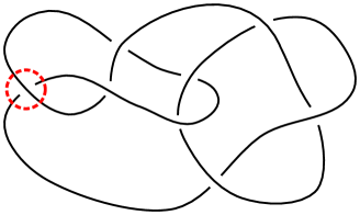
The manifold is surgery on the torus knot of genus 2. The corresponding surgery cobordism provides the form . As we saw at the start of this section, the canonical positive definite plumbing bounded by is isomorphic to . Next, we observe from Figure 2 that the torus knot is obtained from the torus knot by a positive crossing change. This induces a cobordism from +1 surgery on the latter to that of the former with intersection form . (This is a technique used extensively in [CG88].) Attaching to this cobordism the plumbing bounded by yields . Finally, connect summing these three examples with copies of yields all lattices listed in Theorem 1.1, except for .
The author is aware of two constructions realizing . The first has been communicated to the author by Motoo Tange and uses Kirby calculus. The second appears in the author’s work with Golla [GS18], and uses the topology of rational cuspidal curves. ∎
The proof of Theorem 1.1 only uses input from instanton theory and some algebra. Some of the work may be supplemented by the -invariant, as done in Section 3.2 for Theorem 1.3. Combining work of Ni and Wu [NW15, Prop.1.6] and Rasmussen [Ras04, Thm.2.3] gives the inequalities
| (24) |
where is surgery on the knot . If , then as in the case , the only possible non-diagonal definite lattices that can occur, up to diagonal summands, are the 14 listed in Table 1. Using Corollary 3.1 and Lemma 3.2, of those 14 only , , and can possibly occur. We then only need to compute , both of which are short computations contained in the proof of Lemma 4.2. Alternatively, we may just as easily compute .
5 More examples
The question of which unimodular definite lattices arise from smooth 4-manifolds with no 2-torsion in their homology bounded by a fixed homology 3-sphere only depends on the homology cobordism class of . It is natural to wonder whether we can find linearly independent elements in the homology cobordism group all of which bound the same set of definite unimodular lattices. If one restricts to homology cobordism classes that only bound diagonal lattices, one needs only examine the infinitely generated kernels of the invariants and , for example.
We may then consider classes that bound the same lattices as the Poincaré sphere. For this, recall that Furuta [Fur90] and Fintushel and Stern [FS90] used instantons to show that the family for is an infinite linearly independent set in . The manifold is surgery on a genus 1 twist knot with half twists. However, not all of these classes can bound the same lattices as . Indeed, the Rochlin invariant of is congruent to (mod 2), so the lattice cannot occur when is even. In fact, here is an example where the list of lattices is the same as that of the Poincaré sphere except for :
Corollary 5.1.
If a smooth, compact, oriented and definite 4-manifold with no 2-torsion in its homology has boundary , then its intersection form is equivalent to one of
and all of these possiblities occur.
There are two ways to see that bounds the lattice . For one, its canonical positive definite plumbing graph is given as follows:
The unmarked nodes represent vectors of square , and together form a sublattice isomorphic to ; thus the lattice must be isomorphic to . Alternatively, we note that the twist knot with half twists is obtained from the torus knot by a changing a positive crossing to a negative crossing, and argue as in the proof of Corollary 4.3. We note that both arguments generalize to show that bounds .
One might hope for examples of bounding when is odd other than . The determination of all such seems to be an open problem, but has been studied by Tange, who shows [Tan16, Thm. 1.7] that this is the case for and .
Corollary 5.2.
The linearly independent elements for , bound the same definite unimodular lattices arising from smooth 4-manifolds with no 2-torsion.
Tange has informed the author that this list may be enlarged to include . Yet another example that bounds the same set of lattices as the Poincaré sphere is the Brieskorn sphere , whose positive definite plumbing graph is , and which is surgery on the knot of smooth 4-ball genus 1.
In the introduction it was mentioned that , obtained from surgery on the torus knot of genus 3, is a natural candidate to consider beyond Theorem 1.1. Here the Heegaard Floer -invariant is , so the only possible non-diagonal reduced definite lattices that can occur are those in Table 1. We expect most of these lattices are ruled out by Theorem 2.1. We show in [GS18] that the lattices , , , and occur. As the proofs there use the topology of rational cuspidal curves, here we only explain how to realize , , and .
First, is realized by the surgery cobordism as in all previous examples. Next, the rank 15 lattice arises as the lattice of the positive definite plumbing bounding , given by:
The unmarked nodes have weight . Indeed, viewing as the subset of consisting of vectors whose coordinates sum to zero, the lattice may be defined as
where and superscripts denote repeated entries. Then the top weight 3 node in the plumbing graph represents , and the other nodes are the 14 roots of of the form with the far left entry equal to zero. Finally, the lattices and occur because there is a 2-handle cobordism from to with intersection form . Indeed, the (3,4) torus knot is transformed into the torus knot by changing a positive crossing as in Figure 3, as similarly done in the proof of Corollary 1.4.
Finally, consider again the family , obtained from surgery on the family of torus knots. The initial cases and provided our main examples for Theorems 1.1 and 1.3. The methods in this article alone seem unable to treat the general case. However, we know that the definite lattices
| (25) |
and their sums with are bounded by ; the first is the surgery cobordism, and the rest follow from the fact that the torus knot is obtained from the torus knot by changing positive crossings. These are certainly not all the possible lattices: because bounds , for the 3-manifold bounds . Even if we ignore the issue of diagonal summands, the list is not complete. For example, it is shown in [GS18, Prop.4.14] that bounds the lattice .
6 Relations for a circle times a surface
In this section we discuss the relations that appear in the table of Section 2 and in the proofs of Theorems 2.1 and 2.2. In particular, we prove Proposition 2.3, and reduce the verification of the general relations (mod 2) and (mod 4) to a concrete arithmetic problem.
We define to be the instanton homology, with integer coefficients, of a circle times a surface of genus with a -bundle that has second Stiefel-Whitney class Poincaré dual to the circle factor. More precisely, is the -graded group of Muñoz, which is the quotient of the -graded group by an involution ; see the discussion in [Frø04, §10]. Each of these is endowed with a ring structure using the maps induced by pairs of pants cobordisms times . There is a map
| (26) |
which defines relative Donaldson invariants for the 4-manifold with suitable bundle data. Let be the point class and be a symplectic basis of such that . The mapping class group of acts on , and the three elements
| (27) |
generate the invariant part over the rationals; Muñoz gives a presentation which is recursive in the genus [Mn99, §4]. Our definition of is one half of that from loc. cit.; see Section 7.2 for this justification. The ring has similarly defined elements, which we denote by , of respective -gradings 2, 4, 6. The involution acting on is a ring homomorphism and shifts gradings by 4 (mod 8); the equivalence classes of in are of course .
Lemma 6.1.
Suppose a polynomial is a relation in . If the corresponding polynomial in is of homogeneous -grading, then it is a relation in .
Proof.
If the quotient polynomial is a relation, for some within . Since is of degree 4, and has homogeneous -grading, . ∎
When proving our inequalities, we will need to use relations in . Lemma 6.1 says that so long as they are homogeneously -graded in it suffices to show the corresponding relations in . This is the case for the relations we consider, and henceforth we restrict our attention to .
Let be the moduli space of projectively flat connections on a -bundle with fixed odd determinant over a surface of genus . Muñoz’s work shows that is isomorphic to , and in fact the ring structure of the former is a deformation of the latter. More precisely, the product in is equal to the cup product in up to lower order terms of equal mod 4 gradings. Furthermore, the isomorphism is well-defined over the rationals, so we may replace by . There is also a Morse-Bott spectral sequence, due to Fukaya [Fuk96], starting at and converging to . Since is torsion-free, as proven by Atiyah and Bott [AB83, Thm. 9.10], and the spectral sequence collapses over , it must collapse for all coefficient fields. Thus we obtain
Proposition 6.2.
is torsion-free.
However, the ring structure of is substantially more complicated than that of , since do no generate the invariant part of . This is already true for , which requires more generators than does , see [AB83, §9]. Nonetheless, the relations we are interested in can be extracted from Muñoz’s presentation, which we now recall: set , and recursively define
Each is a polynomial with integer coefficients in . Then the ideal is a complete set of relations for the invariant part of , see [Mn99, Thm.16, Prop.20].
Lemma 6.3.
(mod 8).
Proof.
The corresponding relation holds in . Indeed, the degree 4 element
is integral, see [SS, Eq.(7), Prop.2.4]; it is the second Chern class of the push-forward of a universal bundle. Multiplying both sides by , and a mod 8 inverse for , yields (mod 8) in the ring . Since the product in is a deformation of the product in respecting mod 4 gradings, within we have (mod 8), where is some constant. There is a map induced by a cobordism which contracts handles, cf. [Mn99, Lemma 9]. For , we have (mod 8) since in the relations and follow from and . Thus (mod 8) and the relation follows. ∎
This lemma allows us to write for some element . Define the double factorial for odd. We propose the following.
Conjecture 6.4.
is a polynomial in with integer coefficients. Furthermore, the reduction of this polynomial modulo 4 is congruent to .
The verification of this conjecture implies the relations (mod 2) and (mod 4) within . Indeed, the polynomial in the conjecture is a relation in , since according to Muñoz it is a relation in , and is torsion-free. Its reduction modulo 4 implies the relation (mod 4), which by Lemma 6.3 implies the two desired relations.
In fact, for the purposes of Theorems 2.1 and 2.2, less is required: one only needs to show that the desired relations hold in the quotient ring defined by modding out the elements from . Thus we may set in the recursive equation to define with . Then is a polynomial in and . As we only are concerned with relations modulo 2 and 4, to prove that and it suffices to show that the rational coefficients of all have reduced fraction forms with odd denominators, and have numerators divisible by 4, except for the coefficient in front of , which is odd.
Proof of Proposition 2.3.
Finally, we remark that (mod 2) is a relation in the ring by work of the author with M. Stoffregen [SS]. The above scheme suggests an alternative route to proving this relation. Indeed, the ring has its own recursive presentation, which inspired the work of Muñoz; in the recursive definition of above, simply remove the term . Then Conjecture 6.4 may be formulated with these modified polynomials. In particular, we suspect that the relation (mod 4) also holds in .
In [SS] it is also proven that (mod 2) within . This provides an alternative proof to the first part of Lemma 4.1, which says . Indeed, since is a deformation of the ring , the deformations being of lower degree but homogeneous mod 4, then if is nonzero in the latter, it must also be so in the former.
Table 3
7 Adapting Frøyshov’s argument
We now proceed to the proofs of Theorems 2.1 and 2.2. These are adaptations of Frøyshov’s argument as given in [Frø04], which we closely follow and modify accordingly to the settings of and coefficients. For the technical details of the argument we refer to loc. cit. In the final subsection we discuss some other adaptations.
7.1 Proofs of Theorems 2.1 and 2.2
Let be a smooth, closed, oriented 4-manifold. For now we also assume . Suppose and let be pairwise disjoint embedded surfaces with of genus such that . Let be the result of replacing a tubular neighborhood of with for each . Upon orienting and the exceptional sphere in the corresponding copy of , we form two internal connected sums between and , one preserving orientations, the other reversing. Now define a smooth -dimensional family of metrics where on the closed 4-manifold , which as stretches along a link of . Since , each such link may be identified with .
Let be the -bundle with and . We require to be induced from an element in which is extremal. Denote by the moduli space of projectively -anti-self-dual connections on , and let denote the disjoint union of over . After perturbing, the irreducible stratum is a smooth and possibly non-compact manifold of dimension . Thus
| (28) |
If , then has no reducibles, while contains a finite number. Denote by the result of removing small neighborhoods of each reducible; in particular, if . The assumption that is extremal rules out bubbling off of reducible solutions in these moduli spaces.
We now introduce some notation. Recall from [DK90, §5.1.2] that the -map is given by
| (29) |
Here is a -bundle over a 4-manifold , and is the universal adjoint bundle over , where is the configuration space of connections on . The basepoint fibration associated to is the restriction of to a slice . For later use, we also write
| (30) |
When defining (relative) Donaldson invariants on 4-manifolds, one cuts down moduli spaces inside using geometrically constructed divisors representing -classes. Henceforth we write for the point class. Returning to the setup of the previous paragraph, to any , subset and nonnegative integers for we use the shorthand for the intersection of with generic geometric representatives for supported away from where varies, as runs over . Also, let denote the intersection of with a geometric representative depending on for , where the basepoint is in the location of the stretched link of as . For the constructions see [Frø04, §7], where is called . We similarly define the intersections and for the second Stiefel-Whitney class. For the geometric representative of see (39). For the proof of Theorems 2.1 and 2.2 we need the following, for a general 4-manifold with bundle .
Lemma 7.1.
If has (mod 2), then defines a class in .
Proof.
This follows from [AMR95, Lemma 3]. The proof is short so we include it. By assumption, , so we can lift to a bundle such that . Now use and the decomposition to compute . The result follows. ∎
This lemma reduces to Corollary 5.2.7 of [DK90] when (mod 2). When cutting down moduli spaces by , for as in the lemma, the geometric representatives we have in mind are those constructed as in loc. cit. using line bundles of coupled twisted Dirac operators over the surface.
Proof of Theorem 2.1.
Let be in the complement of the classes, and such that (mod 2) for each ; in the notation of Section 2, the duals of the are contained in . Further assume that (mod 2) where . Now suppose for contradiction that the statement of Theorem 2.1 is not true for this data, i.e.
| (31) |
Set . Using the notation for geometric intersections introduced above, we define the following smooth, unoriented 1-manifold with boundary and a finite number of non-compact ends:
| (32) |
Indeed, the dimension is computed using (28) and the fact that cutting down by each of the classes , and reduces dimension by . It makes sense to cut down by in this setting of coefficients by Lemma 7.1.
The boundary points of arise from the deleted neighborhoods of reducibles in . Denote by the torsion subgroup of . Then each pair corresponds to many reducibles; here, for a splitting into line bundles. The neighborhood of each reducible in is a cone on a complex projective space of dimension . To a reducible associated to , let be the degree two generator of the projective space which is the link of this cone. Then by [DK90, Prop. 5.1.21] we have
| (33) |
From this information and (32) we compute the number of boundary points:
| (34) |
the last congruence holding by our assumptions. Although the signs in the definition of do not matter here, for later cases they do; we refer to [Frø04] for more details regarding orientations.
Now we discuss the ends of (32). These arise as the metric family parameters go off to . Transversality ensures that at most one such parameter can stay unbounded for a given sequence of instantons in . The part of with fixed is a finite number of points, which by gluing theory is a product of instantons over and over . We may write
| (35) |
where counts instantons over , and over . Here is the -graded instanton cohomology of a circle times a surface as discussed in Section 6.
A priori, the elements and only define cochains in their Floer cochain complexes. The unperturbed Chern-Simons functional for the restricted bundle over is Morse-Bott along its critical set, which is two copies of where . According to Thaddeus [Tha00], the manifold has a perfect Morse function. We perturb the Chern-Simons functional so that its critical set consists of two copies of the critical points of such a function. The rank of the instanton Floer cochain complex coincides with that of , and so has zero differential. Thus and may also be viewed as Floer cohomology classes, as claimed in the previous paragraph. In this way we remove the restriction in [Frø04] that all but one of the surfaces have genus 1.
The class comes from in the expression (32), and so (mod 2), in the notation of Section 6. By the definition of and Lemma 6.1, the element is in the ideal of generated by -classes of loops. Just as in the argument of [Frø04, §10], we conclude (35) vanishes mod 2, essentially because (relative) Donaldson invariants involving -classes of loops vanish for 4-manifolds with ; see Section 7.2 for this justification. But then our cut down moduli space (32) has an even number ends and, by (34), an odd number of boundary points, a contradiction.
We make two final remarks. First, although we worked with a homogeneous element in the dual of , the argument easily extends to any linear combination of such elements. This allows the argument to go through for all the data included in the definition of . Second, the general case reduces to that of by surgering loops as in [Frø04, Prop.2].∎
Proof of Theorem 2.2.
We explain how to modify the proof of Theorem 2.1. First, assume is odd and . Let be such that (mod 2), and , where and (mod 2). Lemma 7.1 says that each is integral; a similar computation shows that is integral, since is divisible be two. Suppose as in the definition of that (mod 4), where . Next, in place of (31), we suppose for contradiction that
| (36) |
Set . In place of (32) we define the following smooth, orientable 1-manifold with boundary and a finite number of non-compact ends:
| (37) |
The boundary points of (37) are counted via (33) to be (mod 4). On the other hand, using the gluing relation (35) with coefficients, the definition of , and that , which comes from , equals , the number of ends of (37) is zero modulo 4, a contradiction. Finally, the two remarks made at the end of the proof of Theorem 2.1 carry over to this situation.
Now we consider the second part of Theorem 2.2. In this case we suppose is twice an odd number. In the above paragraph, set . Now suppose (36) holds and that (mod 2). Then the count of boundary points becomes (mod 4), while, as before, the number of ends is zero modulo 4, contradicting our assumptions, and completing the proof. ∎
7.2 -classes of loops
We now take a moment to make more precise which geometric representatives for -classes of loops are to be used in the above constructions. We refer to the simplified situation described in [Frø04, Sec.11]. There, a Riemannian 4-manifold with tublular end is considered, equipped with a -bundle that restricts to some oriented surface non-trivially within the tubular end. Fix a loop . Following constructions from [KM95], Frøyshov then associates to three classes in the instanton Floer cohomology of , the restriction of the bundle over to . Roughly, cuts down moduli by the locus of connection classes with holonomy , and cuts down by holonomy . These classes satisfy the relation . It is observed in [Frø04, Sec.11] that and modulo 2-torsion. However, in our constructions above, arises as , which is torsion-free. Thus is an unambiguously defined class over the integers, and is the one which we have in mind when cutting down by -classes of loops over arbitrary coefficient rings.
According to [KM95, §2(ii)], with rational coefficients is equal to what is usually denoted . Thus is an integral class that agrees with , the latter, in general, a priori only defined over the rationals. The map of (26) on a 1-dimensional homology class is now more precisely defined using , from the 4-manifold with appropriate bundle. The independence of the chosen representative for the class follows from [Frø04, Prop.7]. We have now justified our claim, in Section 6, that the class , as we have normalized it, is integral.
We can now also be more precise about the definition of the ring from Sections 2 and 6: it is the quotient of by the ideal generated by elements , defined using the 4-manifold with appropriate bundle, and allowing to range over a symplectic basis of loops for the surface . In particular, this ideal contains .
Finally, we note that with these conventions the proof that vanishes in the proof of Theorem 2.1 now adapts from the argument in [Frø04]: by definition of , we have (mod 2) for some loops in the 4-manifold at hand, and from [Frø04, Prop.7] the latter quantity vanishes. Indeed, in our proof it is assumed that and that has no 2-torsion in its homology, and thus also , implying that the homology class of each is zero mod 2. Similar remarks hold for the proof of Theorem 2.2.
7.3 Other adaptations
Let us first compare the above arguments to that of Theorem 2.5. Set . We then consider the -dimensional part of the linear combination of oriented manifolds
| (38) |
The number of boundary points, which only appear within , is equal to a power of two times , while the number of ends is zero. Here where each . With these modifications, the argument is much the same as before. This handles the case of Theorem 2.5 for a closed 4-manifold, or that for which is the 3-sphere. The more general case follows from this with minor modifications as in [Frø04].
The above argument is also easily adapted to the case in which is replaced by for an odd integer. We will not make use of these variations, but state them out of curiosity. Define
for and . Upon setting , we may consider the 1-dimensional part of (38) a formal linear combination of 1-manifolds; the powers of two in the definitions of the -classes are invertible modulo . The number of boundary points is again up to a power of two, and the number of ends is zero mod . Define by modifying the condition in the definition of that to (mod p). Then we obtain the following.
Theorem 7.2.
Assume the hypotheses of Theorem 2.5 for a closed 4-manifold, and let be an odd integer. Suppose that the order of the torsion subgroup is relatively prime to . Then
If is prime, and the 4-manifold has instead a homology 3-sphere boundary , then the same inequality holds upon adding to the left side , Frøyshov’s instanton invariant defined over .
The modifications needed to deduce the case with a homology 3-sphere boundary from the closed 4-manifold case are completely analogous to those in [Frø04]. Further, we have:
Proposition 7.3.
Let be odd. Then . Equality holds if is prime and .
Proof.
The proof of the first statement is similar to that of Proposition 4.1. It suffices to show that where . We follow [Frø04, Prop.1]. Consider the extremal vector having entries equal to . If is odd then consists of and where there number of signs is even; if is even it consists of where again the number of signs is even. In either case, the signs in are all equal, and is a power of 2, and in particular nonzero mod . Since , we conclude that .
For the second statement, we follow [Mn99, Prop. 20], and use our notation from Section 6. The recursive equation defining yields (mod ). Thus we have where . Inductively, in we obtain the relation
for some . Now since is prime and , the factor has an inverse mod . After multiplying both sides by this inverse, and, if is odd, multiplying by , we obtain the relation (mod ) within , implying . ∎
8 Alternative proofs
The only instanton Floer theory used in the above proofs of Theorems 1.1 and 1.3 is the input from certain relations in the instanton Floer cohomology of a circle times a surface via Theorems 2.1 and 2.2; the instanton homology of homology 3-spheres is not required at all. In this Section we deduce Corollaries 1.2 and 1.4 with this latter framework at heart, with some help from Floer’s exact triangle. While the two approaches complement one another, they also perhaps belong together in a more natural framework as suggested by Frøyshov’s inequality in characteristic zero, Theorem 2.5; we merely scratch the surface here for and coefficients.
For an integer homology 3-sphere , denote by Floer’s instanton (co)homology from [Flo88], defined with coefficients, and using the conventions of [Frø02]. This is a -graded vector space over . There are elements and defined using moduli spaces of insantons with a trivial flat limit at either end of . There is also a degree endomorphism on , denoted , and defined using the second Stiefel-Whitney class of the basepoint fibration, analogous to how the degree 4 endomorphism is defined in [Frø02] on for certain gradings using the first Pontryagin class.
The elements and are induced by (co)chains and defined just as in [Frø02, 2.1], but with -coefficients, which we now review. Recall that the cochain complex is generated by (perturbed) flat irreducible connections mod gauge. We will follow the notation of [Frø02] and write for the moduli space of finite-energy instantons on with flat limit at and at , and with expected dimension lying in . Write . The cochain is then defined to be , where runs through the generators of , and is the trivial connection. Similarly, for a generator .
The map is induced by a degree cochain map on , defined as follows. Let and be generators such that is 2-dimensional. Let be the natural euclidean 3-plane bundle associated to a basepoint . Choose sections and of this bundle which are pulled back from the basepoint fibration over the configuration space of connections on . We arrange that and are linearly dependent at finitely many points, and transversely. Set
| (39) |
That is a chain map, and is independent of any choices made, follows the proof of [Frø02, Thm. 4], except there are no trajectories that break at the reducible. Indeed, since , the relation comes from counting the ends of a 3-dimensional moduli space, cut down by two sections as above; such a moduli space has ends approaching trajectories broken at a trivial connection if its dimension is , see [Don02, §5.1]. The construction of and its interactions with the analogous map for the third Stiefel-Whitney class of was sketched by Frøyshov [Frøa].
Proposition 8.1.
Let be a smooth, compact, oriented 4-manifold with negative definite lattice and boundary an integer homology 3-sphere . If has no -torsion,
The left-hand side is defined entirely in terms of the instanton homology of . The proof is a variation of that for Theorem 2.1. In fact, all that one needs is an analogue of Proposition 1 in [Frø02], which uses the additional assumption that . The analogue is as follows: for descending to an extremal vector of the same name in , and descending to an element of the same name in for some , there is defined a relative Donaldson invariant where , and we have
The statement of Proposition 8.1 follows for from this formula and the definition of ; the condition that is then handled by surgering loops, cf. [Frø04, Prop.2].
We have a similar inequality for coefficients. Here we let denote the degree 4 map defined on as in [Frø02], which in general is not a chain map, but satisfies . The map is a chain map, and we denote by the map obtained after tensoring with and taking homology. This may depend on auxiliary choices, such as perturbation and metric; in the following we assume such choices are fixed.
Proposition 8.2.
Let be a smooth, compact, oriented 4-manifold with negative definite lattice and boundary an integer homology 3-sphere . If has no -torsion,
The proof is similar to that of Proposition 8.1, but more directly uses the formula of [Frø02, Prop.1], the statement of which is the following, assuming ; the proposition uses its mod 4 reduction. For descending to an extremal vector of the same name in , and descending to an element of the same name in for , there is a relative invariant where , and
| (40) |
For both Propositions 8.1 and 8.2 we use the knowledge from Section 7.1 of what kinds of classes can cut down moduli spaces when working over the appropriate coefficient ring. For example, if then is an element in , and the factor is unnecessary in the coefficient ring. A similar statement to that of Proposition 8.2 holds if the 2-torsion in consists of one summand upon replacing with .
We expect that the left-hand sides of the inequalities of Propositions 8.1 and 8.2 can be replaced by more natural quantities. For example, the first of these should be a weaker form of a general inequality involving Frøyshov’s homology cobordism invariant mentioned in the introduction. Similarly, the second is related to Frøyshov’s framework as developed in [Frø02], but with coefficients. We are now in a position to give an alternative proof of Corollary 1.4.
Another proof of Corollary 1.4.
Let . It is well-known that is generated by two flat connections in degrees and . The differential on is zero, and hence is a chain map, and induces a map on which we also call . By [Frø02, Prop.2], is divisible by , and in particular (mod 4) vanishes. The degree two map on is zero for grading reasons. Thus the left-hand sides of the inequalities in Propositions 8.1 and 8.2 are equal to 1, and the result follows from Lemmas 3.2 and 3.3, or from the argument in Section 3.2. ∎
The computation (mod 8) used above is computed in [Frø02] via basic gluing formulae for relative Donaldson invariants, using an embedding of the negative definite plumbing into a surface. The same procedure may be attempted for , the boundary of a negative definite plumbing with intersection form which itself embeds in the elliptic surface , as follows from [FS01, Sec.2], and builds on the construction explained at the beginning of Section 4. However, we can obtain the congruence (mod 8) for the Poincaré sphere by another method, which will also lead to another proof of Corollary 1.2 for , without reverting to gluing formulae for Donaldson invariants. We proceed to explain this.
As in the above proof, let , and denote by the non-trivial -bundle over -surgery on the -torus knot. Then for any coefficient ring we have the long exact sequence
| (41) |
This is Floer’s exact triangle. The map is induced by a surgery 2-handle cobordism . Because the instanton cohomology of the 3-sphere vanishes, is an isomorphism. For the non-trivial bundle , the map is also defined on instanton cohomology. The map does not commute with ; in fact where counts isolated instantons on with trivial limit at . From this it follows, however, that on . Thus to show that (mod 8) on it suffices to show that (mod 8) on .
The (2,3) torus knot has genus 1. Consequently, there is a genus 1 surface embedded in the 0-surgery over which the bundle restricts non-trivially; this is formed by capping off a Seifert surface in the complement of the surgery neighborhood with a disk glued in from -surgery. Following [Frø02, §6] we stretch along a link of this surface in cross the 0-surgery diffeomorphic to a 3-torus to conclude that factors through the corresponding map on . However, on this latter group, (mod 8), establishing the claim. We note that essentially the same argument shows that (mod 8) for the family of Brieskorn spheres , and so we obtain alternative proofs for Corollaries 5.1 and 5.2 as well.
Another proof of Corollary 1.2.
Let . The exact sequence (41) now applies to surgery on the (2,5) torus knot. As for , the Floer complex for has zero differential and is chain map. Again, although and do not commute in general, they do on . Furthermore, and the mod 2 reduction of commute. Next, the torus knot is of genus 2, and has (mod 4) and (mod 2) since (mod 4) and (mod 2) within . Now the left-hand sides of the inequalities in Propositions 8.1 and 8.2 are and , respectively, and with Lemma 4.2 the result follows. ∎
9 The lattice
The root lattice may be described as the subset of consisting of vectors with and all in one of or . The positive definite unimodular lattice is defined by
We note that is cyclic of order 2 generated by . In this section we show
Proposition 9.1.
, and .
Consequently, the inequalities of Theorems 2.1, 2.2 and 2.5 give different genus bounds for the lattice . In the course of the proof to follow we leave some of the computations to the reader.
Proof.
We need to understand the index two cosets of and their extremal vectors. We divide the cosets into two types: those in the image of the inclusion-induced map
and those that are not. To better understand the former case, we list the index two cosets of . These are easily found by hand, and are also listed in [CS99, p.169]. First define
Note that , and . Consider the cosets for . After applying automorphisms of to these we obtain all cosets in . There are cosets in the orbit of , each represented by a vector of square 2, unique up to sign, and there are similarly cosets in the orbit of , each having 12 square 4 vectors. There are only two other cosets, represented by and , which are fixed under the action of the automorphism group. Thus the total number of cosets is , as expected.
The cosets in that lie in the image of are therefore represented by for and some cosets obtained from these by applying automorphisms. The case can be ignored; indeed, , so this vector represents the zero coset. Next we note where has square 2, and , a vector of square 4. Similarly, is mod 2 equivalent to a vector of square 4 supported in . Thus by symmetry, when maximizing over the data defining , and which has extremal and contained in the image of , we may restrict our attention to being among , , , and .
Now we consider cosets not contained in the image of . We claim that upon defining
all elements in are obtained from the cosets represented by , , , , and after perhaps applying an automorphism of . The claim is verified by counting. First note that has 1-dimensional kernel. Indeed, a basis for is given by the rows of the matrix:
Every row in the matrix except for the first lies in , and the first row is equivalent modulo to the vector . Thus every coset not in the image of is of the form where , and there are such cosets.
We consider orbits of the automorphism group acting on as varies through the above representatives. Let be the subgroup of generated by automorphisms that permute the first 8 or last 8 coordinates, the automorphism that swaps the first and last 8 coordinates, and the automorphism that negates the first 8 coordinates. First consider
Then consists of vectors obtained from by permuting the placement of the terms within each -factor and changing signs on each -factor. Thus . The only mod 2 congruences among are , and so . Next, consider
We compute . However, the stabilizer for acting on consists of , the automorphism swapping the first and last 4 coordinates of the second -factor, and any permutation preserving the first 12 coordinates. Taking this into account, we compute . We proceed in this manner to find that for among , , , , and is equal to , , , , and , respectively. These add up to , and this verifies the claim stated in the previous paragraph.
In summary, when maximizing over the data defining , and we may restrict our attention to computing for which is in the following table.
In each case is extremal. We next claim the following, where in each case runs over the vectors in the table: (i) for and for as runs over a basis for ; and (ii) (mod 2) for each with , where are arbitrary elements of a basis for . It is straightforward to verify these claims by computer once one knows for each above. For example, if , this set consists of the vectors obtained by permuting the placement of the terms within each -summand. Claim (i) implies and . More precisely, for the latter, it establishes that , and Lemma 3.2 implies equality. Claim (ii) implies . ∎
The following result collects the lattices that occur in Elkies’ List, Table 1 above, under the constraint . In terms of our topological tools, it combines the restrictions of having -invariant 2 and the mod two inequality of Theorem 2.1 having left-hand side equal to 2. We do not know if the lattice ever occurs under the hypotheses given.
Proposition 9.2.
Suppose is an integer homology 3-sphere with and . If a smooth, compact, oriented 4-manifold with no 2-torsion in its homology has boundary and reduced negative-definite non-diagonal intersection form , then is one of , , .
Proof.
By Proposition 8.1 it suffices to show that for the lattices in Table 1 other than the three given. As in the proof of Lemma 3.3, if the the root lattice contains for , then shows that . This leaves , , , , in Table 1. The following descriptions of the first three of these lattices are from [CS82].
Suppose . This lattice is generated by along with and . As before, superscripts denote repeated entries. Then is extremal of square 4, and , implying .
Next, suppose . Then is generated by and , and . Then is extremal of square 4 and as before .
Next, suppose . Then is generated by along with and , and cyclic permutations of . Then is extremal of square 5 with , implying .
Now suppose . We sketch the construction of this lattice following Construction A of [CS99, Ch.7] using the shortened Golay code . Let be the subspace of the Golay code consisting of vectors with first two coordinates 00 or 11, where is spanned by the rows of Fig. 3.4 in [CS99, p.84]. Then is the subspace of obtained by projecting onto the last 22 coordinates, and is the subset of consisting of vectors such that (mod 2) lies in . Let descend to the code word (mod 2) in with 10 entries equal to , obtained by summing the first 11 rows of Fig. 3.4 in [CS99, p.84], ignoring the first two coordinates. Then is extremal of square 5. It is straightforward to verify that any extremal vector equivalent to is of the form for a root . The roots are the elements with one nonzero entry equal to . From this we obtain , implying .
Finally, suppose , the shorter Leech lattice. Let be any vector of square 5; such a vector exists by inspecting the theta-series of , as given in (7) of [CS99, p.443]. Using that has no roots, , and . ∎
References
- [AB83] M. F. Atiyah and R. Bott. The Yang-Mills equations over Riemann surfaces. Philos. Trans. Roy. Soc. London Ser. A, 308(1505):523–615, 1983.
- [AMR95] Selman Akbulut, Tom Mrowka, and Yongbin Ruan. Torsion classes and a universal constraint on Donaldson invariants for odd manifolds. Trans. Amer. Math. Soc., 347(1):63–76, 1995.
- [BG] Stefan Behrens and Marco Golla. Heegaard Floer correction terms, with a twist. Quantum Topol., 9(1), 1–37, 2018.
- [CG88] Tim D. Cochran and Robert E. Gompf. Applications of Donaldson’s theorems to classical knot concordance, homology -spheres and property . Topology, 27(4):495–512, 1988.
- [CS82] J. H. Conway and N. J. A. Sloane. On the enumeration of lattices of determinant one. J. Number Theory, 15(1):83–94, 1982.
- [CS99] J. H. Conway and N. J. A. Sloane. Sphere packings, lattices and groups, volume 290 of Grundlehren der Mathematischen Wissenschaften [Fundamental Principles of Mathematical Sciences]. Springer-Verlag, New York, third edition, 1999. With additional contributions by E. Bannai, R. E. Borcherds, J. Leech, S. P. Norton, A. M. Odlyzko, R. A. Parker, L. Queen and B. B. Venkov.
- [DK90] S. K. Donaldson and P. B. Kronheimer. The geometry of four-manifolds. Oxford Mathematical Monographs. The Clarendon Press, Oxford University Press, New York, 1990. Oxford Science Publications.
- [Don86] S. K. Donaldson. Connections, cohomology and the intersection forms of -manifolds. J. Differential Geom., 24(3):275–341, 1986.
- [Don02] S. K. Donaldson. Floer homology groups in Yang-Mills theory, volume 147 of Cambridge Tracts in Mathematics. Cambridge University Press, Cambridge, 2002. With the assistance of M. Furuta and D. Kotschick.
- [Ebe13] Wolfgang Ebeling. Lattices and codes. Advanced Lectures in Mathematics. Springer Spektrum, Wiesbaden, third edition, 2013. A course partially based on lectures by Friedrich Hirzebruch.
- [Elk95a] Noam D. Elkies. A characterization of the lattice. Math. Res. Lett., 2(3):321–326, 1995.
- [Elk95b] Noam D. Elkies. Lattices and codes with long shadows. Math. Res. Lett., 2(5):643–651, 1995.
- [Flo88] Andreas Floer. An instanton-invariant for -manifolds. Comm. Math. Phys., 118(2):215–240, 1988.
- [Frøa] Kim Frøyshov. Lecture at the University of Regensburg. July 2016.
- [Frøb] Kim A. Frøyshov. On Floer Homology and Four-Manifolds with Boundary. PhD Thesis.
- [Frø02] Kim A. Frøyshov. Equivariant aspects of Yang-Mills Floer theory. Topology, 41(3):525–552, 2002.
- [Frø04] Kim A. Frøyshov. An inequality for the -invariant in instanton Floer theory. Topology, 43(2):407–432, 2004.
- [Frø10] Kim A. Frøyshov. Monopole Floer homology for rational homology 3-spheres. Duke Math. J., 155(3):519–576, 2010.
- [FS88] Ronald Fintushel and Ronald J. Stern. Definite -manifolds. J. Differential Geom., 28(1):133–141, 1988.
- [FS90] Ronald Fintushel and Ronald J. Stern. Instanton homology of Seifert fibred homology three spheres. Proc. London Math. Soc. (3), 61(1):109–137, 1990.
- [FS01] Ronald Fintushel and Ronald Stern. The canonical class of a symplectic 4-manifold. Turkish J. Math., 25(1):137–145, 2001.
- [Fuk96] Kenji Fukaya. Floer homology of connected sum of homology -spheres. Topology, 35(1):89–136, 1996.
- [Fur90] Mikio Furuta. Homology cobordism group of homology -spheres. Invent. Math., 100(2):339–355, 1990.
- [GS18] Marco Golla and Christopher Scaduto. On definite lattices bounded by integer surgeries along knots with slice genus at most 2. arXiv:1807.11931.
- [KM95] P. B. Kronheimer and T. S. Mrowka. Embedded surfaces and the structure of Donaldson’s polynomial invariants. J. Differential Geom., 41(3):573–734, 1995.
- [Man16] Ciprian Manolescu. Pin(2)-equivariant Seiberg-Witten Floer homology and the triangulation conjecture. J. Amer. Math. Soc., 29(1):147–176, 2016.
- [Mn99] Vicente Muñoz. Ring structure of the Floer cohomology of . Topology, 38(3):517–528, 1999.
- [NV03] Gabriele Nebe and Boris Venkov. Unimodular lattices with long shadow. J. Number Theory, 99(2):307–317, 2003.
- [NW15] Yi Ni and Zhongtao Wu. Cosmetic surgeries on knots in . J. Reine Angew. Math., 706:1–17, 2015.
- [OS03] Peter Ozsváth and Zoltán Szabó. Absolutely graded Floer homologies and intersection forms for four-manifolds with boundary. Adv. Math., 173(2):179–261, 2003.
- [Ras04] Jacob Rasmussen. Lens space surgeries and a conjecture of Goda and Teragaito. Geom. Topol., 8:1013–1031, 2004.
- [SS] Christopher Scaduto and Matthew Stoffregen. The cohomology of rank two stable bundle moduli: mod two nilpotency & skew Schur polynomials. arXiv:1707.06207.
- [Tan16] Motoo Tange. The -boundings of homology spheres and negative sphere classes in . Topology Appl., 202:160–182, 2016.
- [Tha00] Michael Thaddeus. A perfect Morse function on the moduli space of flat connections. Topology, 39(4):773–787, 2000.