BourGAN: Generative Networks with Metric Embeddings

Abstract

This paper addresses the mode collapse for generative adversarial networks (GANs). We view modes as a geometric structure of data distribution in a metric space. Under this geometric lens, we embed subsamples of the dataset from an arbitrary metric space into the $\ell_{2}$ space, while preserving their pairwise distance distribution. Not only does this metric embedding determine the dimensionality of the latent space automatically, it also enables us to construct a mixture of Gaussians to draw latent space random vectors. We use the Gaussian mixture model in tandem with a simple augmentation of the objective function to train GANs. Every major step of our method is supported by theoretical analysis, and our experiments on real and synthetic data confirm that the generator is able to produce samples spreading over most of the modes while avoiding unwanted samples, outperforming several recent GAN variants on a number of metrics and offering new features.

1 Introduction

In unsupervised learning, Generative Adversarial Networks (GANs) [1] is by far one of the most widely used methods for training deep generative models. However, difficulties of optimizing GANs have also been well observed  [2, 3, 4, 5, 6, 7, 8]. One of the most prominent issues is mode collapse, a phenomenon in which a GAN, after learning from a data distribution of multiple modes, generates samples landed only in a subset of the modes. In other words, the generated samples lack the diversity as shown in the real dataset, yielding a much lower entropy distribution.

We approach this challenge by questioning two fundamental properties of GANs. i) We question the commonly used multivariate Gaussian that generates random vectors for the generator network. We show that in the presence of separated modes, drawing random vectors from a single Gaussian may lead to arbitrarily large gradients of the generator, and a better choice is by using a mixture of Gaussians. ii) We consider the geometric interpretation of modes, and argue that the modes of a data distribution should be viewed under a specific distance metric of data items – different metrics may lead to different distributions of modes, and a proper metric can result in interpretable modes. From this vantage point, we address the problem of mode collapse in a general metric space. To our knowledge, despite the recent attempts of addressing mode collapse [3, 9, 10, 6, 11, 12], both properties remain unexamined.

Technical contributions.

We introduce BourGAN, an enhancement of GANs to avoid mode collapse in any metric space. In stark contrast to all existing mode collapse solutions, BourGAN draws random vectors from a Gaussian mixture in a low-dimensional latent space. The Gaussian mixture is constructed to mirror the mode structure of the provided dataset under a given distance metric. We derive the construction algorithm from metric embedding theory, namely the Bourgain Theorem [13]. Not only is using metric embeddings theoretically sound (as we will show), it also brings significant advantages in practice. Metric embeddings enable us to retain the mode structure in the $\ell_{2}$ latent space despite the metric used to measure modes in the dataset. In turn, the Gaussian mixture sampling in the latent space eases the optimization of GANs, and unlike existing GANs that assume a user-specified dimensionality of the latent space, our method automatically decides the dimensionality of the latent space from the provided dataset.

To exploit the constructed Gaussian mixture for addressing mode collapse, we propose a simple extension to the GAN objective that encourages the pairwise $\ell_{2}$ distance of latent-space random vectors to match the distance of the generated data samples in the metric space. That is, the geometric structure of the Gaussian mixture is respected in the generated samples. Through a series of (nontrivial) theoretical analyses, we show that if BourGAN is fully optimized, the logarithmic pairwise distance distribution of its generated samples closely match the logarithmic pairwise distance distribution of the real data items. In practice, this implies that mode collapse is averted.

We demonstrate the efficacy of our method on both synthetic and real datasets. We show that our method outperforms several recent GAN variants in terms of generated data diversity. In particular, our method is robust to handle data distributions with multiple separated modes – challenging situations where all existing GANs that we have experimented with produce unwanted samples (ones that are not in any modes), whereas our method is able to generate samples spreading over all modes while avoiding unwanted samples.

2 Related Work

GANs and variants.

The main goal of generative models in unsupervised learning is to produce samples that follow an unknown distribution $\mathcal{X}$, by learning from a set of unlabelled data items $\{x_{i}\}_{i=1}^{n}$ drawn from $\mathcal{X}$. In recent years, Generative Adversarial Networks (GANs) [1] have attracted tremendous attention for training generative models. A GAN uses a neural network, called generator $G$, to map a low-dimensional latent-space vector $z\in\mathbb{R}^{d}$, drawn from a standard distribution $\mathcal{Z}$ (e.g., a Gaussian or uniform distribution), to generate data items in a space of interest such as natural images and text. The generator $G$ is trained in tandem with another neural network, called the discriminator $D$, by solving a minmax optimization with the following objective.

$$L_{\textrm{gan}}(G,D)=\mathbb{E}_{x\sim\mathcal{X}}\left[\log{D(x)}\right]+\mathbb{E}_{z\sim\mathcal{Z}}\left[\log(1-D(G(z)))\right].$$ (1)

This objective is minimized over $G$ and maximized over $D$. Initially, GANs are demonstrated to generate locally appreciable but globally incoherent images. Since then, they have been actively improving. For example, DCGAN [8] proposes a class of empirically designed network architectures that improve the naturalness of generated images. By extending the objective (1), InfoGAN [14] is able to learn interpretable representations in latent space, Conditional GAN  [15] can produce more realistic results by using additional supervised label. Several later variants have applied GANs to a wide array of tasks  [16, 17] such as image-style transfer [18, 19], super-resolution [20], image manipulation [21], video synthesis [22], and 3D-shape synthesis [23], to name a few.

\begin{overpic}[width=433.62pt]{figs/largegradient.pdf} \put(17.3,-1.7){(a)} \put(50.9,-1.7){(b)} \put(84.0,-1.7){(c)} \end{overpic}

Figure 1: Multi-mode challenge. We train a generator $G$ that maps a latent-space distribution $\mathcal{Z}$ to the data distribution $\mathcal{X}$ with two modes. (a) Suppose $\mathcal{Z}$ is a Gaussian, and $G$ can fit both modes. If we draw two i.i.d. samples $z_{1},z_{2}$ from $\mathcal{Z}$, then with at least a constant probability, $G(z_{1})$ is close to the center $x_{1}$ of the first mode, and $G(z_{2})$ is close to another center $x_{2}$. By the Mean Value Theorem, there exists a $z$ between $z_{1}$ and $z_{2}$ that has the absolute gradient value, $|G^{\prime}(z)|=|\frac{x_{2}-x_{1}}{z_{2}-z_{1}}|$, which can be arbitrarily large, as $|x_{2}-x_{1}|$ can be arbitrarily far. (b) Since $G$ is Lipschitz continuous, using it to map a Gaussian distribution to both modes unavoidably results in unwanted samples between the modes (highlighted by the red dots). (c) Both challenges are resolved if we can construct a mixture of Gaussian in latent space that captures the same modal structure as in the data distribution.

Addressing difficulties.

Despite tremendous success, GANs are generally hard to train. Prior research has aimed to improve the stability of training GANs, mostly by altering its objective function [24, 4, 25, 26, 27, 28]. In a different vein, Salimans et al. [3] proposed a feature-matching technique to stabilize the training process, and another line of work [5, 6, 29] uses an additional network that maps generated samples back to latent vectors to provide feedback to the generator.

A notable problem of GANs is mode collapse, which is the focus of this work. For instance, when trained on ten hand-written digits (using MNIST dataset) [30], each digit represents a mode of data distribution, but the generator often fails to produce a full set of the digits [25]. Several approaches have been proposed to mitigate mode collapse, by modifying either the objective function [4, 12] or the network architectures [9, 5, 11, 10, 31]. While these methods are evaluated empirically, theoretical understanding of why and to what extent these methods work is often lacking. More recently, PacGAN [11] introduces a mathematical definition of mode collapse, which they used to formally analyze their GAN variant. Very few previous works consider the construction of latent space: VAE-GAN [29] constructs the latent space using variational autoencoder, and GLO [32] tries to optimize both the generator network and latent-space representation using data samples. Yet, all these methods still draw the latent random vectors from a multivariate Gaussian.

Differences from prior methods.

Our approach differs from prior methods in several important technical aspects. Instead of using a standard Gaussian to sample latent space, we propose to use a Gaussian mixture model constructed using metric embeddings (e.g., see [33, 34, 35] for metric embeddings in both theoretical and machine learning fronts). Unlike all previous methods that require the latent-space dimensionality to be specified a priori, our algorithm automatically determines its dimensionality from the real dataset. Moreover, our method is able to incorporate any distance metric, allowing the flexibility of using proper metrics for learning interpretable modes. In addition to empirical validation, the steps of our method are grounded by theoretical analysis.

3 Bourgain Generative Networks

We now introduce the algorithmic details of BourGAN, starting by describing the rationale behind the proposed method. The theoretical understanding of our method will be presented in the next section.

Rationale and overview.

We view modes in a dataset as a geometric structure embodied under a specific distance metric. For example, in the widely tested MNIST dataset, only two modes emerge under the pixel-wise $\ell_{2}$ distance (Fig. 2-left): images for the digit “1” are clustered in one mode, while all other digits are landed in another mode. In contrast, under the classifier distance metric (defined in Appx. F.3), it appears that there exist 10 modes each corresponding to a different digit. Consequently, the modes are interpretable (Fig. 2-right). In this work, we aim to incorporate any distance metric when addressing mode collapse, leaving the flexibility of choosing a specific metric to the user.

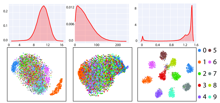
Figure 2: (Top) Pairwise distance distribution on MNIST dataset under different distance metrics. Left: $\ell_{2}$ distance, Middle: Earth Mover’s distance (EMD) with a quadratic ground metric, Right: classifier distance (defined in Appx. F.3). Under $\ell_{2}$ and EMD distances, few separated modes emerges, and the pairwise distance distributions resemble a Gaussian. Under the classifier distance, the pairwise distance distribution becomes bimodal, indicating that there are separated modes. (Bottom) t-SNE visualization [36] of data items after embedded from their metric space to $\ell_{2}$ space. Color indicates labels of MNIST images (“1”-“9”). When $\ell_{2}$ distance (left) is used, only two modes are identified: digit “1” and all others, but classifier distance (right) can group data items into 10 individual modes.

When there are multiple separated modes in a data distribution, mapping a Gaussian random variable in latent space to the data distribution is fundamentally ill-posed. For example, as illustrated in Fig. 1-a and 1-b, this mapping imposes arbitrarily large gradients (at some latent space locations) in the generator network, and large gradients render the generator unstable to train, as pointed out by [37].

A natural choice is to use a mixture of Gaussians. As long as the Gaussian mixture is able to mirror the mode structure of the given dataset, the problem of mapping it to the data distribution becomes well-posed (Fig. 1-c). To this end, our main idea is to use metric embeddings, one that map data items under any metric to a low-dimensional $\ell_{2}$ space with bounded pairwise distance distortion (Sec. 3.3). After the embedding, we construct a Gaussian mixture in the $\ell_{2}$ space, regardless of the distance metric for the data items. In this process, the dimensionality of the latent space is also automatically decided.

Our embedding algorithm, building upon the Bourgain Theorem, requires us to compute the pairwise distances of data items, resulting in an $O(n^{2})$ complexity, where $n$ is the number of data items. When $n$ is large, we first uniformly subsample $m$ data items from the dataset to reduce the computational cost of our metric embedding algorithm (Sec. 3.2). The subsampling step is theoretically sound: we prove that when $m$ is sufficiently large yet still much smaller than $n$, the geometric structure (i.e., the pairwise distance distribution) of data items is preserved in the subsamples.

Lastly, when training a BourGAN, we encourage the geometric structure embodied in the latent-space Gaussian mixture to be preserved by the generator network. Thereby, the mode structure of the dataset is learned by the generator. This is realized by augmenting GAN’s objective to foster the preservation of the pairwise distance distribution in the training process (Sec. 3.4).

3.1 Metrics of Distance and Distributions

Before delving into our method, we introduce a few theoretical tools to concretize the geometric structure in a data distribution, paving the way toward understanding our algorithmic details and subsequent theoretical analysis. In the rest of this paper, we borrow a few notational conventions from theoretical computer science: we use $[n]$ to denote the set $\{1,2,\cdots,n\}$, $\mathbb{R}_{\geq 0}$ to denote the set of all non-negative real numbers, and $\log(\cdot)$ to denote $\log_{2}(\cdot)$ for short.

Metric space.

A metric space is described by a pair $(\mathbb{M},\operatorname*{d})$, where $\mathbb{M}$ is a set and $\operatorname*{d}:\mathbb{M}\times\mathbb{M}\rightarrow\mathbb{R}_{\geq 0}$ is a distance function such that $\forall x,y,z\in\mathbb{M},$ we have i) $\operatorname*{d}(x,y)=0\Leftrightarrow x=y,$ ii) $\operatorname*{d}(x,y)=\operatorname*{d}(y,x),$ and iii) $\operatorname*{d}(x,z)\leq\operatorname*{d}(x,y)+\operatorname*{d}(y,z).$ If $\mathbb{M}$ is a finite set, then we call $(\mathbb{M},\operatorname*{d})$ a finite metric space.

Wasserstein-$1$ distance.

Wasserstein-$1$ distance, also known as the Earth-Mover distance, is one of the distance measures to quantify the similarity of two distributions, defined as $W(\mathcal{P}_{a},\mathcal{P}_{b})=\inf_{\Gamma\in\Pi(\mathcal{P}_{a},\mathcal{P}_{b})}\operatorname*{{\mathbb{E}}}_{(x,y)\sim\Gamma}\left(|x-y|\right),$ where $\mathcal{P}_{a}$ and $\mathcal{P}_{b}$ are two distributions on real numbers, and $\Pi(\mathcal{P}_{a},\mathcal{P}_{b})$ is the set of all joint distributions $\Gamma(x,y)$ on two real numbers whose marginal distributions are $\mathcal{P}_{a}$ and $\mathcal{P}_{b}$, respectively. Wasserstein-$1$ distance has been used to augment GAN’s objective and improve training stability [4]. We will use it to understand the theoretical guarantees of our method.

Logarithmic pairwise distance distribution (LPDD).

We propose to use the pairwise distance distribution of data items to reflect the mode structure in a dataset (Fig. 2-top). Since the pairwise distance is measured under a specific metric, its distribution also depends on the metric choice. Indeed, it has been used in [9] to quantify how well Unrolled GAN addresses mode collapse.

Concretely, given a metric space $(\operatorname*{{\mathbb{M}}},\operatorname*{d})$, let $\mathcal{X}$ be a distribution over $\operatorname*{{\mathbb{M}}}$, and $(\lambda,\Lambda)$ be two real values satisfying $0<2\lambda\leq\Lambda$. Consider two samples $x,y$ independently drawn from $\mathcal{X}$, and let $\eta$ be the logarithmic distance between $x$ and $y$ (i.e., $\eta=\log(\operatorname*{d}(x,y))$). We call the distribution of $\eta$ conditioned on $\operatorname*{d}(x,y)\in[\lambda,\Lambda]$ the $(\lambda,\Lambda)-$logarithmic pairwise distance distribution (LPDD) of the distribution $\mathcal{X}$. Throughout our theoretical analysis, LPDD of the distributions generated at various steps of our method will be measured in Wasserstein-$1$ distance.

Remark. We choose to use logarithmic distance in order to reasonably compare two pairwise distance distributions. The rationale is illustrated in Fig. 6 in the appendix. Using logarithmic distance is also beneficial for training our GANs, which will become clear in Sec. 3.4. The $(\lambda,\Lambda)$ values in the above definition are just for the sake of theoretical rigor, irrelevant from our practical implementation. They are meant to avoid the theoretical situation where two samples are identical and then taking the logarithm becomes no sense. In this section, the reader can skip these values and refer back when reading our theoretical analysis (in Sec. 4 and the supplementary material).

3.2 Preprocessing: Subsample of Data Items

We now describe how to train BourGAN step by step. Provided with a multiset of data items $X=\{x_{i}\}_{i=1}^{n}$ drawn independently from an unknown distribution $\mathcal{X}$, we first subsample $m$ ($m<n$) data items uniformly at random from $X$. This subsampling step is essential, especially when $n$ is large, for reducing the computational cost of metric embeddings as well as the number of dimensions of the latent space (both described in Sec. 3.3). From now on, we use $Y$ to denote the multiset of data items subsampled from $X$ (i.e., $Y\subseteq X$ and $|Y|=m$). Elements in $Y$ will be embedded in $\ell_{2}$ space in the next step.

The subsampling strategy, while simple, is theoretically sound. Let $\mathcal{P}$ be the $(\lambda,\Lambda)$-LPDD of the data distribution $\mathcal{X}$, and $\mathcal{P}^{\prime}$ be the LPDD of the uniform distribution on $Y$. We will show in Sec. 4 that their Wasserstein-$1$ distance $W(\mathcal{P},\mathcal{P}^{\prime})$ is tightly bounded if $m$ is sufficiently large but much smaller than $n$. In other words, the mode structure of the real data can be captured by considering only the subsamples in $Y$. In practice, $m$ is chosen automatically by a simple algorithm, which we describe in Appx. F.1. In all our examples, we find $m=4096$ sufficient.

3.3 Construction of Gaussian Mixture in Latent Space

Next, we construct a Gaussian mixture model for generating random vectors in latent space. First, we embed data items from $Y$ to an $\ell_{2}$ space, one that the latent random vectors reside in. We want the latent vector dimensionality to be small, while ensuring that the mode structure be well reflected in the latent space. This requires the embedding to introduce minimal distortion on the pairwise distances of data items. For this purpose, we propose an algorithm that leverages Bourgain’s embedding theorem.

Metric embeddings.

Bourgain [13] introduced a method that can embeds any finite metric space into a small $\ell_{2}$ space with minimal distortion. The theorem is stated as follows:

Theorem 1 (Bourgain’s theorem).

Consider a finite metric space $(Y,\operatorname*{d})$ with $m=|Y|.$ There exists a mapping $g:Y\rightarrow\mathbb{R}^{k}$ for some $k=O(\log^{2}m)$ such that $\forall y,y^{\prime}\in Y,\operatorname*{d}(y,y^{\prime})\leq\|g(y)-g(y^{\prime})\|_{2}\leq\alpha\cdot\operatorname*{d}(y,y^{\prime})$, where $\alpha$ is a constant satisfying $\alpha\leq O(\log m)$.

The mapping $g$ is constructed using a randomized algorithm also given by Bourgain [13]. Directly applying Bourgain’s theorem results in a latent space of $O(\log^{2}m)$ dimensions. We can further reduce the number of dimensions down to $O(\log m)$ through the following corollary.

Corollary 2 (Improved Bourgain embedding).

Consider a finite metric space $(Y,\operatorname*{d})$ with $m=|Y|.$ There exist a mapping $f:Y\rightarrow\mathbb{R}^{k}$ for some $k=O(\log m)$ such that $\forall y,y^{\prime}\in Y,\operatorname*{d}(y,y^{\prime})\leq\|f(y)-f(y^{\prime})\|_{2}\leq\alpha\cdot\operatorname*{d}(y,y^{\prime})$, where $\alpha$ is a constant satisfying $\alpha\leq O(\log m).$

Proved in Appx. B, this corollary is obtained by combining Thm. 1 with the Johnson-Lindenstrauss (JL) lemma [38]. The mapping $f$ is computed through a combination of the algorithms for Bourgain’s theorem and the JL lemma. This algorithm of computing $f$ is detailed in Appx. A.

Remark. Instead of using Bourgain embedding, one can find a mapping $f:Y\rightarrow\mathbb{R}^{k}$ with bounded distortion, namely, $\forall y,y^{\prime}\in Y,\operatorname*{d}(y,y^{\prime})\leq\|f(y)-f(y^{\prime})\|_{2}\leq\alpha\cdot\operatorname*{d}(y,y^{\prime})$, by solving a semidefinite programming problem (e.g., see [39, 33]). This approach can find an embedding with the least distortion $\alpha$. However, solving semidefinite programming problem is much more costly than computing Bourgain embeddings. Even if the optimal distortion factor $\alpha$ is found, it can still be as large as $O(\log m)$ in the worst case [40]. Indeed, Bourgain embedding is optimal in the worst case.

Using the mapping $f$, we embed data items from $Y$ (denoted as $\{y_{i}\}_{i=1}^{m}$) into the $\ell_{2}$ space of $k$ dimensions ($k=O(\log m)$). Let $F$ be the multiset of the resulting vectors in $\mathbb{R}^{k}$ (i.e., $F=\{f(y_{i})\}_{i=1}^{m}$). As we will formally state in Sec. 4, the Wasserstein-$1$ distance between the $(\lambda,\Lambda)-$LPDD of the real data distribution $\mathcal{X}$ and the LPDD of the uniform distribution on $F$ is tightly bounded. Simply speaking, the mode structure in the real data is well captured by $F$ in $\ell_{2}$ space.

Latent-space Gaussian mixture.

Now, we construct a distribution using $F$ to draw random vectors in latent space. A simple choice is the uniform distribution over $F$, but such a distribution is not continuous over the latent space. Instead, we construct a mixture of Gaussians, each of which is centered at a vector $f(y_{i})$ in $F$. In particular, we generate a latent vector $z\in\mathbb{R}^{k}$ in two steps: We first sample a vector $\mu\in F$ uniformly at random, and then draw a vector $z$ from the Gaussian distribution $\mathcal{N}(\mu,\sigma^{2})$, where $\sigma$ is a smoothing parameter that controls the smoothness of the distribution of the latent space. In practice, we choose $\sigma$ empirically ($\sigma=0.1$ for all our examples). We discuss our choice of $\sigma$ in Appx. F.1.

Remark. By this definition, the Gaussian mixture consists of $m$ Gaussians (recall $F=\{f(y_{i})\}_{i=1}^{m}$). But this does not mean that we construct $m$ “modes” in the latent space. If two Gaussians are close to each other in the latent space, they should be viewed as if they are from the same mode. It is the overall distribution of the $m$ Gaussians that reflects the distribution of modes. In this sense, the number of modes in the latent space is implicitly defined, and the $m$ Gaussians are meant to enable us to sample the modes in the latent space.

3.4 Training

The Gaussian mixture distribution $\mathcal{Z}$ in the latent space guarantees that the LPDD of $\mathcal{Z}$ is close to $(\lambda,\Lambda)-$LPDD of the target distribution $\mathcal{X}$ (shown in Sec. 4). To exploit this property for avoiding mode collapse, we encourage the generator network to match the pairwise distances of generated samples with the pairwise $\ell_{2}$ distances of latent vectors in $\mathcal{Z}$. This is realized by a simple augmentation of the GAN’s objective function, namely,

$$L(G,D)=L_{\textrm{gan}}+\beta L_{\textrm{dist}},\;$$ (2)

$$\textrm{where}\;L_{\textrm{dist}}(G)=\mathbb{E}_{z_{i},z_{j}\sim\mathcal{Z}}\left[\left(\log({d(G(z_{i}),G(z_{j}))})-\log({\|z_{i}-z_{j}\|_{2}})\right)^{2}\right],$$ (3)

$L_{\textrm{gan}}$ is the objective of the standard GAN in Eq. (1), and $\beta$ is a parameter to balance the two terms. In $L_{\textrm{dist}}$, $z_{i}$ and $z_{j}$ are two i.i.d. samples from $\mathcal{Z}$ conditioned on $z_{i}\neq z_{j}$. Here the advantages of using logarithmic distances are threefold: i) When there exists “outlier” modes that are far away from others, logarithmic distance prevents those modes from being overweighted in the objective. ii) Logarithm turns a uniform scale of the distance metric into a constant addend that has no effect to the optimization. This is desired as the structure of modes is invariant under a uniform scale of distance metric. iii) Logarithmic distances ease our theoretical analysis, which, as we will formalize in Sec. 4, states that when Eq. (3) is optimized, the distribution of generated samples will closely resemble the real distribution $\mathcal{X}$. That is, mode collapse will be avoided.

In practice, when experimenting with real datasets, we find that a simple pre-training step using the correspondence between $\{y_{i}\}_{i=1}^{m}$ and $\{f(y_{i})\}_{i=1}^{m}$ helps to improve the training stability. Although not a focus of this paper, this step is described in Appx. C.

4 Theoretical Analysis

This section offers an theoretical analysis of our method presented in Sec. 3. We will state the main theorems here while referring to the supplementary material for their rigorous proofs. Throughout, we assume a property of the data distribution $\mathcal{X}$: if two samples, $a$ and $b$, are drawn independently from $\mathcal{X}$, then with a high probability ($>\nicefrac{{1}}{{2}}$) they are distinct (i.e., $\Pr_{a,b\sim\mathcal{X}}(a\not=b)\geq\nicefrac{{1}}{{2}}$).

Range of pairwise distances.

We first formalize our definition of $(\lambda,\Lambda)-$LPDD in Sec. 3.1. Recall that the multiset $X=\{x_{i}\}_{i=1}^{n}$ is our input dataset regarded as i.i.d. samples from $\mathcal{X}$. We would like to find a range $[\lambda,\Lambda]$ such that the pairwise distances of samples from $\mathcal{X}$ is in this range with a high probability (see Example-7 and -8 in Appx. D). Then, when considering the LPDD of $\mathcal{X}$, we account only for the pairwise distances in the range $[\lambda,\Lambda]$ so that the logarithmic pairwise distance is well defined. The values $\lambda$ and $\Lambda$ are chosen by the following theorem, which we prove in Appx. G.2.

Theorem 3.

Let $\lambda=\min_{i\in[n-1]:x_{i}\not=x_{i+1}}\operatorname*{d}(x_{i},x_{i+1})$ and $\Lambda=\max_{i\in[n-1]}\operatorname*{d}(x_{i},x_{i+1})$. $\forall\delta,\gamma\in(0,1)$, if $n\geq C/(\delta\gamma)$ for some sufficiently large constant $C>0$, then with probability at least $1-\delta,$ $\Pr_{a,b\sim\mathcal{X}}(\operatorname*{d}(a,b)\in[\lambda,\Lambda]\mid\lambda,\Lambda)\geq\Pr_{a,b\sim\mathcal{X}}(a\not=b)-\gamma.$

Simply speaking, this theorem states that if we choose $\lambda$ and $\Lambda$ as described above, then we have $\Pr_{a,b\sim\mathcal{X}}(\operatorname*{d}(a,b)\in[\lambda,\Lambda]\mid a\not=b)\geq 1-O(\nicefrac{{1}}{{n}})$, meaning that if $n$ is large, the pairwise distance of any two i.i.d. samples from $\mathcal{X}$ is almost certainly in the range $[\lambda,\Lambda]$. Therefore, $(\lambda,\Lambda)-$LPDD is a reasonable measure of the pairwise distance distribution of $\mathcal{X}$. In this paper, we always use $\mathcal{P}$ to denote the $(\lambda,\Lambda)-$LPDD of the real data distribution $\mathcal{X}$.

Number of subsamples.

With the choices of $\lambda$ and $\Lambda$, we have the following theorem to guarantee the soundness of our subsampling step described in Sec. 3.2.

Theorem 4.

Let $Y=\{y_{i}\}_{i=1}^{m}$ be a multiset of $m=\log^{O(1)}(\Lambda/\lambda)\cdot\log(1/\delta)$ i.i.d. samples drawn from $\mathcal{X}$, and let $\mathcal{P}^{\prime}$ be the LPDD of the uniform distribution on $Y$. For any $\delta\in(0,1),$ with probability at least $1-\delta,$ we have $W(\mathcal{P},\mathcal{P}^{\prime})\leq O(1).$

Proved in Appx. G.3, this theorem states that we only need $m$ (on the order of $\log^{O(1)}(\Lambda/\lambda)$) subsamples to form a multiset $Y$ that well captures the mode structure in the real data.

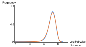
Figure 3: LPDD of uniform distribution $\mathcal{F}$ (orange) and of samples from Gaussian mixture (blue).

Discrete latent space.

Next, we lay a theoretical foundation for our metric embedding step described in Sec. 3.3. Recall that $F$ is the multiset of vectors resulted from embedding data items from $Y$ to the $\ell_{2}$ space (i.e., $F=\{f(y_{i})\}_{i=1}^{m})$. As proved in Appx. G.4, we have:

Theorem 5.

Let $\mathcal{F}$ be the uniform distribution on the multiset $F$. Then with probability at least $0.99$, we have $W(\mathcal{P},\hat{\mathcal{P}})\leq O(\log\log\log(\Lambda/\lambda)),$ where $\hat{\mathcal{P}}$ is the LPDD of $\mathcal{F}$.

Here the triple-log function ($\log\log\log(\Lambda/\lambda)$) indicates that the Wasserstein distance bound can be very tight. Although this theorem states about the uniform distribution on $F$, not precisely the Gaussian mixture we constructed, it is about the case when $\sigma$ of the Gaussian mixture approaches zero. We also empirically verified the consistency of LPDD from Gaussian mixture samples (Fig. 3).

GAN objective.

Next, we theoretically justify the objective function (i.e., Eq. (3) in Sec. 3.4). Let $\mathcal{\tilde{X}}$ be the distribution of generated samples $G(z)$ for $z\sim\mathcal{Z}$ and $\mathcal{\tilde{P}}$ be the $(\lambda,\Lambda)-$LPDD of $\mathcal{\tilde{X}}$. Goodfellow et al. [1] showed that the global optimum of the GAN objective (1) is reached if and only if $\mathcal{\tilde{X}}=\mathcal{X}$. Then, when this optimum is achieved, we must also have $W(\mathcal{P},\mathcal{\tilde{P}})=0$ and $W(\mathcal{\tilde{P}},\mathcal{\hat{P}})\leq O(\log\log\log(\Lambda/\lambda))$. The latter is because $W(\mathcal{P},\mathcal{\hat{P}})\leq O(\log\log\log(\Lambda/\lambda))$ from Thm. 5.

As a result, the GAN’s minmax problem (1) is equivalent to the constrained minmax problem, $\min_{G}\max_{D}L_{\textrm{gan}}(G,D)$, subject to $W(\mathcal{\tilde{P}},\mathcal{\hat{P}})\leq\beta$, where $\beta$ is on the order of $O(\log\log\log(\Lambda/\lambda))$. Apparently, this constraint renders the minmax problem harder. We therefore consider the minmax problem, $\min_{G}\max_{D}L_{\textrm{gan}}(G,D)$, subjected to slightly strengthened constraints,

$$\forall z_{1}\not=z_{2}\in\operatorname*{supp}(\mathcal{Z}),\operatorname*{d}(G(z_{1}),G(z_{2}))\in[\lambda,\Lambda],\,\,\textrm{and}$$ (4)

$$\left[\log(\operatorname*{d}(G(z_{1}),G(z_{2})))-\log\|z_{1}-z_{2}\|_{2}\right]^{2}\leq\beta^{2}.$$ (5)

As proved in Appx. E, if the above constraints are satisfied, then $W(\mathcal{\tilde{P}},\mathcal{\hat{P}})\leq\beta$ is automatically satisfied. In our training process, we assume that the constraint (4) is automatically satisfied, supported by Thm. 3. Lastly, instead of using Eq. (5) as a hard constraint, we treat it as a soft constraint showing up in the objective function (3). From this perspective, the second term in our proposed objective (2) can be interpreted as a Lagrange multiplier of the constraint.

LPDD of the generated samples.

Now, if the generator network is trained to satisfy the constraint (5), we have $W(\mathcal{\tilde{P}},\mathcal{\hat{P}})\leq O(\log\log\log(\Lambda/\lambda))$. Note that this satisfaction does not imply that the global optimum of the GAN in Eq. (1) has to be reached – such a global optimum is hard to achieve in practice. Finally, using the triangle inequality of the Wasserstein-$1$ distance and Thm. 5, we reach the conclusion that

$$W(\tilde{\mathcal{P}},\mathcal{P})\leq W(\tilde{\mathcal{P}},\hat{\mathcal{P}})+W(\mathcal{P},\hat{\mathcal{P}})\leq O(\log\log\log(\Lambda/\lambda)).$$ (6)

This means that the LPDD of generated samples closely resembles that of the data distribution. To put the bound in a concrete context, in Example 9 of Appx. D, we analyze a toy case in a thought experiment to show, if the mode collapse occurs (even partially), how large $W(\tilde{\mathcal{P}},\mathcal{P})$ would be in comparison to our theoretical bound here.

5 Experiments

This section presents the empirical evaluations of our method. There has not been a consensus on how to evaluate GANs in the machine learning community [41, 42], and quantitative measure of mode collapse is also not straightforward. We therefore evaluate our method using both synthetic and real datasets, most of which have been used by recent GAN variants. We refer the reader to Appx. F for detailed experiment setups and complete results, while highlighting our main findings here.

	2D Ring			2D Grid			2D Circle
	#modes (max 8)	$\mathcal{W}_{1}$	low quality	#modes (max 25)	$\mathcal{W}_{1}$	low quality	center captured	$\mathcal{W}_{1}$	low quality
GAN	1.0	38.60	0.06%	17.7	1.617	17.70%	No	32.59	0.14%
Unrolled	7.6	4.678	12.03%	14.9	2.231	95.11%	No	0.360	0.50%
VEEGAN	8.0	4.904	13.23%	24.4	0.836	22.84%	Yes	0.466	10.72%
PacGAN	7.8	1.412	1.79%	24.3	0.898	20.54%	Yes	0.263	1.38%
BourGAN	8.0	0.687	0.12%	25.0	0.248	4.09%	Yes	0.081	0.35%

Table 1: Statistics of Experiments on Synthetic Datasets

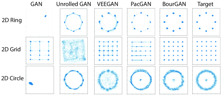
Figure 4: Synthetic data tests. In all three tests, our method clearly captures all the modes presented in the targets, while producing no unwanted samples located between the regions of modes.

Overview.

We start with an overview of our experiments. i) On synthetic datasets, we quantitatively compare our method with four types of GANs, including the original GAN [1] and more recent VEEGAN [10], Unrolled GANs [9], and PacGAN [11], following the evaluation metrics used by those methods (Appx. F.2). ii) We also examine in each mode how well the distribution of generated samples matches the data distribution (Appx. F.2) – a new test not presented previously. iii) We compare the training convergence rate of our method with existing GANs (Appx. F.2), examining to what extent the Gaussian mixture sampling is beneficial. iv) We challenge our method with the difficult stacked MNIST dataset (Appx. F.3), testing how many modes it can cover. v) Most notably, we examine if there are “false positive” samples generated by our method and others (Fig. 4). Those are unwanted samples not located in any modes. In all these comparisons, we find that BourGAN clearly produces higher-quality samples. In addition, we show that vi) our method is able to incorporate different distance metrics, ones that lead to different mode interpretations (Appx. F.3); and vii) our pre-training step (described in Appx. C) further accelerates the training convergence in real datasets (Appx. F.2). Lastly, viii) we present some qualitative results (Appx. F.4).

Quantitative evaluation.

We compare BourGAN with other methods on three synthetic datasets: eight 2D Gaussian distributions arranged in a ring (2D Ring), twenty-five 2D Gaussian distributions arranged in a grid (2D Grid), and a circle surrounding a Gaussian placed in the center (2D Circle). The first two were used in previous methods [9, 10, 11], and the last is proposed by us. The quantitative performance of these methods are summarized in Table 1, where the column “# of modes” indicates the average number of modes captured by these methods, and “low quality” indicates number of samples that are more than $3\times$ standard deviations away from the mode centers. Both metrics are used in previous methods [10, 11]. For the 2D circle case, we also check if the central mode is captured by the methods. Notice that all these metrics measure how many modes are captured, but not how well the data distribution is captured. To understand this, we also compute the Wasserstein-$1$ distances between the distribution of generated samples and the data distribution (reported in Table 1). It is evident that our method performs the best on all these metrics (see Appx. F.2 for more details).

Avoiding unwanted samples.

A notable advantage offered by our method is the ability to avoid unwanted samples, ones that are located between the modes. We find that all the four existing GANs suffer from this problem (see Fig. 4), because they use Gaussian to draw latent vectors (recall Fig. 1). In contrast, our method generates no unwanted samples in all three test cases. We refer the reader to Appx. F.3 for a detailed discussion of this feature and several other quantitative comparisons.

Qualitative results.

We further test our algorithm on real image datasets. Fig. 5 illustrates a qualitative comparison between DCGAN and our method, both using the same generator and discriminator architectures and default hyperparameters. Appx. F.4 includes more experiments and details.

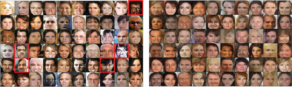
Figure 5: Qualitative results on CelebA dataset using DCGAN (Left) and BourGAN (Right) under $\ell_{2}$ metric. It appears that DCGAN generates some samples that are visually more implausible (e.g., red boxes) in comparison to BourGAN. Results are fairly sampled at random, not cherry-picked.

6 Conclusion

This paper introduces BourGAN, a new GAN variant aiming to address mode collapse in generator networks. In contrast to previous approaches, we draw latent space vectors using a Gaussian mixture, which is constructed through metric embeddings. Supported by theoretical analysis and experiments, our method enables a well-posed mapping between latent space and multi-modal data distributions. In future, our embedding and Gaussian mixture sampling can also be readily combined with other GAN variants and even other generative models to leverage their advantages.

Acknowledgements

We thank Daniel Hsu, Carl Vondrick and Henrique Maia for the helpful feedback. Chang Xiao and Changxi Zheng are supported in part by the National Science Foundation (CAREER-1453101, 1717178 and 1816041) and generous donations from SoftBank and Adobe. Peilin Zhong is supported in part by National Science Foundation (CCF-1703925, CCF-1421161, CCF-1714818, CCF-1617955 and CCF-1740833), Simons Foundation (#491119 to Alexandr Andoni) and Google Research Award.

Algorithm 1 Improved Bourgain Embedding

  Input: A finite metric space $(Y,\operatorname*{d}).$

  Output: A mapping $f:Y\rightarrow\mathbb{R}^{O(\log|Y|)}$.

  //Bourgain Embedding:

  Initialization: $m\leftarrow|Y|,$ $t\leftarrow O(\log m),$ and $\forall i\in[\lceil\log m\rceil],j\in[t],S_{i,j}\leftarrow\emptyset.$

  for $i=1\rightarrow\lceil\log m\rceil$ do

     for $j=1\rightarrow t$ do

        For each $x\in Y,$ independently choose $x$ in $S_{i,j},$ i.e. $S_{i,j}=S_{i,j}\cup\{x\}$ with probability $2^{-i}.$

     end for

  end for

  Initialize $g:Y\rightarrow\mathbb{R}^{\lceil\log m\rceil\cdot t}.$

  for $x\in Y$ do

     $\forall i\in[\lceil\log m\rceil],j\in[t],$ set the $((i-1)\cdot t+j)$-th coordinate of $g(x)$ as $\operatorname*{d}(x,S_{i,j}).$

  end for

  //Johnson-Lindenstrauss Dimentionality Reduction:

  Let $d=O(\log m)$, and let $G\in\mathbb{R}^{d\times(\lceil\log m\rceil\cdot t)}$ be a random matrix with entries drawn from i.i.d. $\mathcal{N}(0,1).$

  Let $h:\mathbb{R}^{\lceil\log m\rceil\cdot t}\rightarrow\mathbb{R}^{d}$ satisfy $\forall x\in\mathbb{R}^{\lceil\log m\rceil\cdot t},h(x)\leftarrow G\cdot x.$

  //Rescaling:

  Let $\beta=\min_{x,y\in Y:x\not=y}\frac{\|h(g(x))-h(g(y))\|_{2}}{\operatorname*{d}(x,y)}.$

  Initialize $f:Y\rightarrow\mathbb{R}^{d}.$ For $x\in Y,$ set $f(x)\leftarrow h(g(x))/\beta.$

  Return $f$.

\begin{overpic}[width=433.62pt]{figs/lpdd.pdf} \put(10.3,-1.7){(a)} \put(42.9,-1.7){(b)} \put(81.0,-1.7){(c)} \end{overpic}

Figure 6: Intuition of using LPDD. (a) Here blue points illustrate a dataset with three modes. The orange points indicate the same data but uniformly scaled up. (b) The pairwise distance distributions of both datasets are different. The distribution of orange points is a streched version of the distribution of blue points. As a result, the Wasserstein-$1$ distance between both distributions can become arbitrarily large, depending on the scale. (c) In contrast, the distribution of logarithmic pairwise distance remains the same up to a constant shift. In this case, the Wasserstein-$1$ distance of the logarithmic pairwise distance distributions is differed by only a constant addent, which can be easily accounted.

Appendix A Algorithm of Improved Bourgain Embedding

Algorithm 1 outlines our randomized algorithm that computes the improved Bourgain embedding with high probability. To embed a finite metric space $(Y,\operatorname*{d})$ into $\ell_{2}$ space, Algorithm 1 takes $O(m^{2}\cdot s+m^{2}\log^{2}m)$ running time, where $m=|Y|$ is the size of $Y$, and $s$ is the running time needed to compute a pairwise distance $\operatorname*{d}(x,y)$ for any $x,y\in Y.$

Appendix B Proof of Corollary 2

Here we prove the Corollary 2 introduced in Sec. 3.3. First, we recall the Johnson-Lindenstrauss lemma [38].

Theorem 6 (Johnson-Lindenstrauss lemma).

Consider a set of $m$ points $X=\{x_{i}\}_{i=1}^{m}$ in a vector space $\mathbb{R}^{t}$. There exist a mapping $h:X\rightarrow\mathbb{R}^{k}$ for some $k=O(\log m)$ such that

$$\forall i,j\in[m],\|h(x_{i})-h(x_{j})\|_{2}\leq\|x_{i}-x_{j}\|_{2}\leq O(1)\cdot\|h(x_{i})-h(x_{j})\|_{2}.$$

By combining this lemma with Bourgain’s theorem 1, we reach the corollary through the following proof.

Proof.

By Theorem 1, we can embed all data items from $Y$ into the $\ell_{2}$ space with $O(\log^{2}m)$ dimensions and with $O(\log m)$ distortion. Then, according to Theorem 6, we can further reduce the number of dimensions to $O(\log m)$ with $O(\log m)$ distortion. ∎

Appendix C Pre-training

While our method addresses mode collapse, in practice, we have to confront other challenges of training the GAN, particularly its instability and sensitivity to hyper-parameters. To this end, we pre-train the generator network $G$ and use it to warm start the training of our GAN. Pre-training is made possible because our metric embedding step has established the correspondence between the embedding vectors $f(y_{i})$ in the latent space and the data items $y_{i}\in Y$, $i\in[m]$. This correspondence allows us to perform a supervised learning to minimize the objective

$$L_{\textrm{pre}}(G)=\mathbb{E}_{y_{i},z_{i}}\left[d(G(f(y_{i})),y_{i})\right].$$

As will be shown in our experiments, this pre-training step leads to faster convergence when we train our GANs. Lastly, we note that our method can be straightforwardly combined with other objective function extensions [24, 4, 25, 26, 27, 43] and network architectures [11, 44, 9], ones that specifically focus on addressing other challenges such as instability, to leverage their advantages.

Appendix D Illustrative Examples for Sec. 4

The following two examples illustrate the ranges of the pairwise distance that can cover a pairwise distance sample with a high probability. They are meant to exemplify the choices of $\lambda$ and $\Lambda$ discussed in Sec. 4.

Example 7.

Consider the set of all points in $\mathbb{R}^{20},$ and the distance measure is chosen to be the Euclidean distance. Let $\mathcal{X}$ be the Gaussian distribution $\mathcal{N}(0,I).$ Suppose we draw two i.i.d. samples $x,y$ form $\mathcal{X},$ then with probability at least $0.99999,$ $\operatorname*{d}(x,y)$ should be in the range $[0.1,10].$

Example 8.

Consider the set of all $256\times 256$ grayscale images, and the brightness of each pixel is described by a number in $\{0,1,2,\cdots,255\}.$ Let $\mathcal{X}$ be a uniform distribution over all the images which contains a cat. Suppose we draw two i.i.d. samples $x,y$ from $\mathcal{X},$ then with probability $1,$ the distance between $x$ and $y$ should be in the range $[1,255\cdot 256\cdot 256]=[1,16777216].$

Next, we show a concrete example in which if the generator produces samples mainly in one mode, then $W(\mathcal{P},\mathcal{\tilde{P}})$ can be as large as $\Omega(\log(\Lambda/\lambda))$, drastically larger than the bound in (6).

Example 9.

Suppose $\operatorname*{{\mathbb{M}}}=A\cup B\subset\mathbb{R}^{d},$ where $A=\{0,1\}^{d}$ is a Hamming cube close to the origin, and $B=\{\nicefrac{{\Lambda}}{{\sqrt{d}}}-1,\nicefrac{{\Lambda}}{{\sqrt{d}}}\}^{d}$ is another Hamming cube far away from the origin (i.e., $\Lambda\gg d$). It is easy to see that $A,B$ are two separated modes. Let $\operatorname*{d}:\operatorname*{{\mathbb{M}}}\times\operatorname*{{\mathbb{M}}}\rightarrow\mathbb{R}_{\geq 0}$ be the Euclidean distance (i.e., $\forall x,y\in\operatorname*{{\mathbb{M}}}$, $\operatorname*{d}(x,y)=\|x-y\|_{2}$), and let $\lambda=1.$ It is easy to see that $\forall x\not=y\in\operatorname*{{\mathbb{M}}},$ we have $\operatorname*{d}(x,y)\in[\lambda,\Lambda].$ Suppose the real data distribution $\mathcal{X}$ is the uniform distribution on $\operatorname*{{\mathbb{M}}}$. Also suppose the distribution of generated samples is $\tilde{\mathcal{X}}$, and the probability that generator $G$ generates samples near the mode $B$ is at most $1/10$. Then, consider the $(\lambda,\Lambda)-$LPDD (denoted by $\mathcal{P}$) of $\mathcal{X}$. If we draw two independent samples from $\mathcal{X}$, then conditioned on this two samples being distinct, with probability at least $\nicefrac{{1}}{{3}}$, they are in different modes. Thus, if we draw a sample $p$ from $\mathcal{P},$ then with probability at least $\nicefrac{{1}}{{3}}$, $p$ is at least $\nicefrac{{\Lambda}}{{2}}$. Now consider the distribution $\tilde{\mathcal{X}}$ of generated samples. Since with probability at least $\nicefrac{{9}}{{10}}$, a sample from $\tilde{\mathcal{X}}$ will land in mode $A$, if we draw two samples from $\tilde{\mathcal{X}},$ then with probability at least $\nicefrac{{4}}{{5}}$, the distance between these two samples is at most $\sqrt{d}$. Thus, the Wasserstein distance is at least $(\nicefrac{{4}}{{5}}-(1-\nicefrac{{1}}{{3}}))\cdot|\log(\frac{\Lambda}{2})-\log\sqrt{d}|\geq 0.1\log(\nicefrac{{\Lambda}}{{\sqrt{d}}})=\Omega(\log(\Lambda/\lambda))$.

Appendix E Strengthened Constraints for GAN’s Minmax Problem

As explained in Sec. 4, introducing the constraint $W(\mathcal{P},\mathcal{P}^{\prime})<\beta$ in the GAN optimization makes the problem harder to solve. Thus, we choose to slightly strengthen the constraint. Observe that if for all $z_{1}\not=z_{2}\in\operatorname*{supp}(\mathcal{Z})$ we have $|\log(\operatorname*{d}(G(z_{1}),G(z_{2})))-\log(\|z_{1}-z_{2}\|_{2})|\leq O(\log\log\log(\Lambda/\lambda))$ and $\operatorname*{d}(G(z_{1}),G(z_{2}))\in[\lambda,\Lambda],$ we have

$$W(\mathcal{\tilde{P}},\mathcal{\hat{P}}) \leq\sum_{z_{1}\not=z_{2}\in\operatorname*{supp}(\mathcal{Z})}\Pr_{Z_{1},Z_{2}\sim\mathcal{Z}}(Z_{1}=z_{1},Z_{2}=z_{2}\mid Z_{1}\not=Z_{2})\cdot\left|\log\left(\frac{\operatorname*{d}(G(z_{1}),G(z_{2}))}{\|z_{1}-z_{2}\|_{2}}\right)\right|$$

$$\leq O(\log\log\log(\Lambda/\lambda)).$$

In other words, if the constraints in (4) and (5) are satisfied, then the constraint $W(\mathcal{P},\mathcal{P}^{\prime})<\beta$ is automatically satisfied. Thus, they are a slightly strengthened version of $W(\mathcal{P},\mathcal{P}^{\prime})<\beta$.

Appendix F Evaluation and Experiment

In this section, we provide details of our experiments, starting with a few implementation details that are worth noting. All our experiments are performed using a Nvidia GTX 1080 Ti Graphics card and implemented in Pytorch [45].

F.1 Parameter setup

As discussed in Sec. 3.2, we randomly sample $m$ data items from the provided the dataset to form the set $Y$ for subsequent metric embeddings. In our implementation, we choose $m$ automatically by using a simple iterative algorithm. Starting from a small $m$ value (e.g., 32), in each iteration we double $m$ and add more samples from the real dataset. We stop the iteration when the pairwise distance distribution of the samples converges under the Wasserstein-1 distance. The termination of this process is guaranteed because of the existence of the theoretical upper bound of $m$ (recall Thm. 4). In all our examples, we found $m=4096$ sufficient. With the chosen $m$, we construct the multiset $Y={y_{i}}_{i=1}^{m}$ by uniformly sampling the dataset $X$. Afterwards, we compute the metric embedding $f(y_{i})$ for each $y_{i}\in Y$, and normalize each vector in $\{f(y_{i})\}_{i=1}^{m}$ by

$$\bar{f}(y_{i})=\frac{f(y_{i})-\mu_{0}}{\sigma_{0}},$$

where $\mu_{0}$ and $\sigma_{0}$ are the average and standard deviation of the entire set $\{f(y_{i})\}_{i=1}^{m}$, respectively.

Two other parameters are needed in our method, namely, $\beta$ in Eq. (2) and the standard deviation $\sigma$ used for the sampling latent Gaussian mixture model (recall Sec. 3.3). In all our experiments, we set $\beta=0.2$ and $\sigma=0.1$. We find that the final mode coverage of generated samples is not sensitive to $\sigma$ value in the range $[0.2,0.6]$. Only when $\sigma$ is too small, the Gaussian mixture becomes noisy (or “spiky”), and when $\sigma$ is too large, the Gaussian mixture starts to degrade into a single Gaussian as used in conventional GANs.

F.2 Experiment Details on Synthetic Data

Setup.

We follow the experiment setup used in [10] for 2D Ring and 2D Grid. In the additional 2D circle case, the input dataset is generated by using 100 Gaussian distributions on a circle with a radius $r=2$, as well as three identical Gaussians located at the center of the circle. All Gaussians have the same standard deviation (i.e., 0.05).

All the GANs (including our method and compared methods) in this experiment share the same generator and discriminator architectures. They have two hidden layers, each of which has 128 units with ReLU activation and without any dropout [46] or normalization layers [47]. When using the Unrolled GAN [9], we set the number of unrolling steps to be five as suggested in the authors’ reference implementation. When using PacGAN [11], we follow the authors’ suggestion and set the number of packing to be four. In all synthetic experiments, our method is performed without the pre-training step described in Sec. C.

During training, we use a mini-batch size of 256 with 3000 iterations in total, and use the Adam [48] optimization method with a learning rate of $0.001$ and set $\beta_{1}=0.5,\beta_{2}=0.999$. During testing, we use 2500 samples from the learned generator network for evaluation, and use $\ell_{2}$ distance as the target distance metric for Bourgain embedding. Every metric value listed in Table 1 is evaluated and averaged over 10 trials.

Studies.

When evaluating the number of captured modes (“# modes” in Table 1), a mode is considered as being “captured” when there exists at least one sample located within one standard-deviation-distance (1-std) away from the center of the mode. This criterion is slightly different from that used in [10, 11], in which they use three standard-deviation (3-std). We choose to use 1-std because we would like to have finer granularity to differentiate the tested GANs in terms of their mode capture performance.

To gain a better understanding of the mode capture performance, we also measure in each method the percentages of generated samples located within 1-, 2-, and 3-std away from mode centers for the three test datasets. The results are reported in Table 2. We note that for Gaussian distribution, the percentages of samples located in 1-, 2-, and 3-std away from the center are 68.2%, 95.4%, 99.7%, respectively [49]. Our method produces results that are closest to these percentages in comparison to other methods. This suggests that our method better captures not only individual modes but also the data distribution in each mode, thanks to the pairwise distance preservation term (3) in our objective function. We also note that this experiment result is echoed by the Wasserstein-$1$ measure reported in Table 1, for which we measure the Wasserstein-$1$ distance between the distribution of generated samples and the true data distribution. Our method under that metric also performs the best.

	2D Ring			2D Grid			2D Circle
	1-std	2-std	3-std	1-std	2-std	3-std	1-std	2-std	3-std
GAN	61.46%	96.14%	99.94%	35.86%	69.86%	82.3%	82.08%	98.26%	99.86%
Unrolled	70.66%	85.09%	87.96%	0.54%	2.10%	4.88%	92.08%	99.35%	99.49%
VEEGAN	51.68%	79.24%	86.76%	24.76%	60.24%	77.16%	54.72%	80.44%	89.28%
PacGAN	88.32%	97.28%	98.20%	28.9%	67.76%	79.46%	58.10%	94.62%	98.62%
BourGAN	59.54%	96.64%	99.88%	38.64%	81.54%	95.9%	67.52%	95.64%	99.64%

Table 2: Statistics of Experiments on Synthetic Datasets

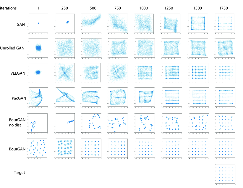
Figure 7: How quickly do they converge? Our method outperforms other methods in terms of convergence rate in this example. From left to right are the samples generated after the generators are trained over an increasing number of iterations. The fifth row indicates the performance of Wasserstein GAN [4], although it is not particularly designed for addressing mode collapse. The sixth row reports the performance of BourGAN with standard GAN objective (i.e., no distance preservation term (3) is used). The seventh row indicate BourGAN with our proposed objective function, which converges in the least number of iterations.

Lastly, we examine how quickly these methods converges during the training process. The results are reported in Fig. 7, where we also include the results from our BourGAN but set $\beta$ in the objective 2 to be zero. That is, we also test our method using standard GAN objective function. Figure 7 shows that our method with augmented objective converges the most quickly: The generator becomes stable after 1000 iterations in this example, while others remain unstable even after 1750 iterations. This result also empirically supports the necessity of using the pairwise distance preservation term in the objective function. We attribute the faster convergence of our method to the fact that the latent-space Gaussian mixture in our method encodes the structure of modes in the data space and the fact that our objective function encourages the generator to preserve this structure.

F.3 Evaluation on MNIST and Stacked MNIST

In this section, we report the evaluation results on MNIST dataset. All MNIST images are scaled to 32$\times$32 by bilinear interpolation.

Setup.

Quantitative evaluation of GANs is known to be challenging, because the implicit distributions of real datasets are hard, if not impossible, to obtain. For the same reason, quantification of mode collapse is also hard for real datasets, and no widely used evaluation protocol has been established. We take an evaluation approach that has been used in a number of existing GAN variants [42, 10, 9]: we use a third-party trained classifier to classify the generated samples into specific modes, and thereby estimate the generator’s mode coverage [3].

Classifier distance.

A motivating observation of our method is that the structure of modes depends on a specific choice of distance metric (recall Fig. 2). The widely used distance metrics on images (such as the pixel-wise $\ell_{2}$ distance and Earth Mover’s distance) may not necessarily produce interpretable mode structures. Here we propose to use the Classifier Distance metric defined as

$$d_{\text{classifier}}(x_{i},x_{j})=\|P(x_{i})-P(x_{j})\|_{2},$$ (7)

where $P(x_{i})$ is the softmax output vector of a pre-trained classification network, and $x_{i}$ represents an input image. Adding a third-party trained classifier turns the task of training generative models semi-supervised [15]. Nevertheless, Eq. (7) is a highly complex distance metric, serving for the purpose of testing our method with an “unconventional” metric. It is also meant to show that a properly chosen metric can produce interpretable modes.

Visualization of embeddings.

After we apply our metric embedding algorithm with different distance metrics on MNIST images, we obtain a set of vectors in $\ell_{2}$ space. To visualize these vectors in 2D, we use t-SNE [36], a nonlinear dimensionality reduction technique well-suited for visualization of high-dimensional data in 2D or 3D. Although not fully accurately, this visualization shreds light on how (and where) data points are located in the latent space (see Fig. 2).

MNIST experiment.

First, we verify that our pre-training step (described in Appx. C) indeed accelerates the training process, as illustrated in Fig. 8.

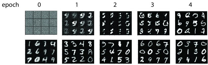
Figure 8: Efficacy of pre-training. (Top) BourGAN without pre-training. (Bottom) BourGAN with pre-training. With the pre-training step, the GAN converges faster, and the generator network produces better-quality results in each epoch.

Next, we evaluate the quality of generated samples using different distance metrics. One widely used evaluation score is the inception score [25] that measures both the visual quality and diversity of generated samples. However, as pointed out by [12], a generative model can produce a high inception score even when it collapses to a visually implausible sample. Furthermore, we would like to measure the visual quality and diversity separately rather than jointly, to understand the performance of our method in each of the two aspects under different metrics. Thus, we choose to use entropy, defined as $E(x)=-\sum_{i=0}^{9}p(y=i|x)\log p(y=i|x)$, as the score to measure the quality of the generated sample $x$, where $p(y=i|x)$ is the probability of labeling the input $x$ as the digit $i$ by the pre-trained classifier. The rationale here is that a high-quality sample often produces a low entropy through the pre-trained classifier.

We compare DCGAN with BourGAN using this score. Since our method can incorporate different distance metrics, we consider two of them: BourGAN using $\ell_{2}$ distance and BourGAN using the aforementioned classifier distance. For a fair comparison, the three GANS (i.e., DCGAN, BourGAN ($\ell_{2}$), and BourGAN (classifier)) all use the same number of dimensions ($k=55$) for the latent space and the same network architecture. For each type of GANs, we randomly generate 5000 samples to evaluate the entropy scores, and the results are reported in Fig. 9. We also compute the KL divergence between the generated distribution and the data distribution, following the practice of [9, 36]. The KL divergence for DCGAN, BourGAN ($\ell_{2}$) and BourGAN (classifier) are 0.116, 0.104, and 0.012, respectively.

A well-trained generator is expected to produce a relatively uniform distribution across all 10 digits. Our experiment suggests that both BourGAN ($\ell_{2}$) and BourGAN (classifier) generate better-quality samples in comparison to DCGAN, as they both produce lower entropy scores (Fig. 9-right). Yet, BourGAN (classifier) has a lower KL divergence compared to BourGAN ($\ell_{2}$), suggesting that the classifier distance is a better metric in this case to learn mode diversity. Although a pre-trained classifier may not always be available in real world applications, here we demonstrate that some metric might be preferred over others depending on the needs, and our method has the flexibility to use different metrics.

Lastly, we show that interpretable modes can be learned when a proper distance metric is chosen. Figure 10 shows the generated images when sampling around individual vectors in latent space. The BourGAN generator trained with $\ell_{2}$ distance tends to produce images that are close to each other under $\ell_{2}$ measure, while the generator trained with classifier distance tends to produce images that are in the same class, which is more interpretable.

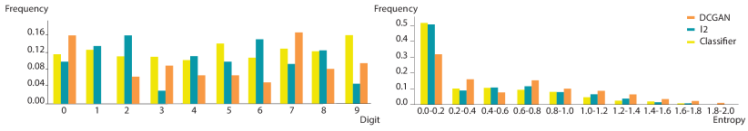
Figure 9: MNIST dataset with different distance metrics. (left) We plot the distribution of digits generated by DCGAN in orange, BourGAN ($\ell_{2}$) in green, and BourGAN (classifier) in yellow. The generated images from those GANs are classified using a pre-trained classifier. This plot shows that the classifier distance produces samples that are most uniformly distributed across all 10 digits. DCGAN fails to capture the mode of digital “1”, while BourGAN ($\ell_{2}$) generates fewer samples for the modes in “3” and “9”. (right) Entropy distribution of generated samples using three GANs. A lower entropy value indicates better image quality. This plot suggests that our method with both $\ell_{2}$ and classifier distance metrics produces higher-quality MNIST images than the DCGAN.

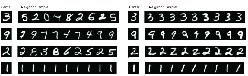
Figure 10: Interpretable modes. Using BourGAN, we first randomly generate four samples and use their latent vectors as four centers in latent space. We then sample nine latent vectors in a hypersphere of each center, and use these vectors to generate MNIST images. The hypersphere has a radius of 0.1 (Left) BourGAN ($\ell_{2}$) generates samples that are close to others in the same hypersphere in $\ell_{2}$ space. But the samples can be visually distinct from each other, representing different digits. Note that under $\ell_{2}$ distance, digit “1” are separated out (the fourth row on the left). It is interesting to recall the bottom-left subfigure of Fig. 2, and realize that this resonates with that subfigure in which data items of digit “1” are clustered as a separated mode in $\ell_{2}$ metric. (Right) BourGAN (classifier) is trained with the classifier distance, which tends to cluster together images that represent the same type of digits. As a result, the generated samples tend to represent the same digits as their respective centers. Thus, the modes captured by BourGAN (classifier) is more interpretable. In this case, each mode corresponds to a different digit.

Tests on Stacked MNIST.

Similar to the evaluation methods in Mode-regularized GANs [12], Unrolled GANs [9], VEEGAN [10] and PacGAN [11], we test BourGAN with $\ell_{2}$ distance metric on an augmented MNIST dataset. By encapsulating three randomly selected MNIST images into three color channels, we construct a new dataset of 100,000 images, each of which has a dimension of 32$\times$32$\times$3. In the end, we obtain 10$\times$10$\times$10 = 1000 distinct classes. We refer to this dataset as the stacked MNIST dataset. In this experiment, we will treat each of the 1000 classes of images as an individual mode.

	D is 1/4 size of G		D is 1/2 size of G		D is same size as G
	# class covered (max 1000)	KL	# class covered (max 1000)	KL	# class covered (max 1000)	KL
DCGAN	92.2	5.02	367.7	4.87	912.3	0.65
BourGAN	715.2	1.84	936.1	0.61	1000.0	0.08

Table 3: Mode coverage on stacked MNIST Dataset. Results are averaged over 10 trials

As reported in [9], even regular GANs can learn all 1000 modes if the discriminator size is sufficiently large. Thus, we evaluate our method by setting the discriminator’s size to be $\nicefrac{{1}}{{4}}\times$, $\nicefrac{{1}}{{2}}\times$, and $1\times$ of the generator’s size, respectively. We measure the number of modes captured by our method as well as by DCGAN, and the KL divergence between the generated distribution of modes and the expected true distribution of modes (i.e., a uniform distribution over the 1000 modes). Table 3 summarizes our results. In Table 2 and 3 of their paper, Lin et al. [11] reported results on similar experiments, although we note that it is hard to directly compare our Table 3 with theirs, because their detailed network setup and the third-part classifier may differ from ours. We summarize our network structures in Table 4 and 5. During training, we use Adam optimization with a learning rate of $10^{-4}$, and set $\beta_{1}=0.5$ and $\beta_{2}=0.999$ with a mini-batch size of 128.

Additionally, in Fig. 11 we show a qualitative comparison between our method and DCGAN on this dataset.

layer	output size	kernel size	stride	BN	activation function
input (dim 55)	55$\times$1$\times$1
Transposed Conv	512$\times$4$\times$4	4	1	Yes	ReLU
Transposed Conv	256$\times$8$\times$8	4	2	Yes	ReLU
Transposed Conv	128$\times$16$\times$16	4	2	Yes	ReLU
Transposed Conv	channel$\times$32$\times$32	4	2	No	Tanh

Table 4: Network structure for generator. channel=3 for Stacked MNIST and channel=1 for MNIST.

layer	output size	kernel size	stride	BN	activation function
input (dim 55)	channel$\times$32$\times$32
Conv	256$\times$16$\times$16	4	2	No	LeakyReLU(0.2)
Conv	256$\times$8$\times$8	4	2	Yes	LeakyReLU(0.2)
Conv	128$\times$4$\times$4	4	2	Yes	LeakyReLU(0.2)
Conv	channel$\times$1$\times$1	4	1	No	Sigmoid

Table 5: Network structure for discriminator.

Figure 11: Qualitative results on stacked MNIST dataset. (Left) Samples from real data distribution. (Middle) Samples generated by DCGAN. (Right) Samples generated by BourGAN. In all three GANs, discriminator network has a size $\nicefrac{{1}}{{4}}\times$ of the generator. DCGAN starts to generate collapsed results, while BourGAN still generates plausible results.

F.4 More Qualitative Results

We also test our algorithm on other popular dataset, including CIFAR-10 [50] and Fashion-MNIST [51]. Figure 12 and 13 illustrate our results on these datasets.

Figure 12: Qualitative results on CIFAR-10.

Figure 13: Qualitative results on Fashion-MNIST.

Appendix G Proofs of the Theorems in Section 4

G.1 Notations and Preliminaries

Before we delve into technical details, we first review some notation and fundamental tools in the theoretical analysis: We use $\mathbf{1}(\mathcal{E})$ to denote an indicator variable on the event $\mathcal{E}$, i.e., if $\mathcal{E}$ happens, then $\mathbf{1}(\mathcal{E})=1$, otherwise, $\mathbf{1}(\mathcal{E})=0$.

The following lemma gives a concentration bound on independent random variables.

Lemma 10 (Bernstein Inequality).

Let $X_{1},X_{2},\cdots,X_{n}$ be $n$ independent random variables. Suppose that $\forall i\in[n],|X_{i}-\operatorname*{{\mathbb{E}}}(X_{i})|\leq M$ almost surely. Then, $\forall t>0,$

$$\Pr\left(\left|\sum_{i=1}^{n}X_{i}-\sum_{i=1}^{n}\operatorname*{{\mathbb{E}}}(X_{i})\right|>t\right)\leq 2\exp\left(-\frac{\frac{1}{2}t^{2}}{\sum_{i=1}^{n}\operatorname*{\mathrm{Var}}(X_{i})+\frac{1}{3}Mt}\right).$$

The next lemma states that given a complete graph with a power of $2$ number of vertices, the edges can be decomposed into perfect matchings.

Lemma 11.

Given a complete graph $G=(V,E)$ with $|V|=m$ vertices, where $m$ is a power of $2$. Then, the edge set $E$ can be decomposed into $m-1$ perfect matchings.

Figure 14: An $8$-vertices complete graph can be decomposed into $7$ perfect matchings

Proof.

Our proof is by induction. The base case has $m=1$. For the base case, the claim is obviously true. Now suppose that the claim holds for $m/2.$ Consider a complete graph $G=(V,E)$ with $m$ vertices, where $m$ is a power of $2$. We can partition vertices set $V$ into two vertices sets $A,B$ such that $|A|=|B|=m/2.$ The edges between $A$ and $B$ together with vertices $A\cup B=V$ compose a complete bipartite graph. Thus, the edges between $A$ and $B$ can be decomposed into $m/2$ perfect matchings. The subgraph of $G$ induced by $A$ is a complete graph with $m/2$ vertices. By our induction hypothesis, the edge set of the subgraph of $G$ induced by $A$ can be decomposed into $m/2-1$ perfect matchings in that induced subgraph. Similarly, the edge set of the subgraph of $G$ induced by $B$ can be also decomposed into $m/2-1$ perfect matchings in that induced subgraph. Notice that any perfect matching in the subgraph induced by $A$ union any perfect matching in the subgraph induced by $B$ is a perfect matching of $G$. Thus, $E$ can be decomposed into $m/2+m/2-1=m-1$ perfect matchings. ∎

G.2 Proof of Theorem 3

In the following, we formally restate the theorem.

Theorem 12.

Consider a metric space $(\operatorname*{{\mathbb{M}}},\operatorname*{d}).$ Let $\mathcal{X}$ be a distribution over $\operatorname*{{\mathbb{M}}}$ which satisfies $\Pr_{a,b\sim\mathcal{X}}(a\not=b)\geq 1/2.$ Let $x_{1},x_{2},\cdots,x_{n}$ be $n$ i.i.d. samples drawn from $\mathcal{X}$. Let $\lambda=\min_{i\in[n-1]:x_{i}\neq x_{i+1}}\operatorname*{d}(x_{i},x_{i+1}),\Lambda=\max_{i\in[n-1]:x_{i}\neq x_{i+1}}\operatorname*{d}(x_{i},x_{i+1}).$ For any given parameters $\delta\in(0,1),\gamma\in(0,1),$ if $n\geq C/(\delta\gamma)$ for some sufficiently large constant $C>0$, then with probability at least $1-\delta,$ $\Pr_{a,b\sim\mathcal{X}}(\operatorname*{d}(a,b)\in[\lambda,\Lambda]\mid\lambda,\Lambda)\geq\Pr_{a,b\sim\mathcal{X}}(a\not=b)-\gamma.$

Proof.

Without of loss of generality, we assume $n$ is an even number. Let $\lambda^{\prime}=\min_{i\in[n/2]:x_{2i-1}\not=x_{2i}}\operatorname*{d}(x_{2i-1},x_{2i}),\Lambda^{\prime}=\max_{i\in[n/2]:x_{2i-1}\not=x_{2i}}\operatorname*{d}(x_{2i-1},x_{2i})$, and $P$, $Q$ be two i.i.d. random variables with distribution $\mathcal{X}$. Then $(x_{1},x_{2}),(x_{3},x_{4}),\cdots,(x_{n-1},x_{n})$ are $n/2$ i.i.d. samples drawn from the same distribution as $(P,Q).$ Let $t=|\{j\in[n/2]\mid x_{2j-1}\not=x_{2j}\}|.$ Suppose $p$ is the probability, $p=\Pr(P\not=Q)$, then we have the following relationship.

$$\Pr_{P,Q,x_{1},\cdots,x_{m}\sim\mathcal{D}}\left(\operatorname*{d}(P,Q)<\lambda^{\prime}\vee\operatorname*{d}(P,Q)>\Lambda^{\prime}\mid P\not=Q\right)$$

$$=~{} \Pr_{P,Q,x_{1},\cdots,x_{m}\sim\mathcal{D}}\left(\operatorname*{d}(P,Q)<\lambda^{\prime}\vee\operatorname*{d}(P,Q)>\Lambda^{\prime}\mid P\not=Q,t\geq pn/2\right)\cdot\Pr(t\geq pn/2\mid P\not=Q)$$ (8)

$$+\Pr_{P,Q,x_{1},\cdots,x_{m}\sim\mathcal{D}}\left(\operatorname*{d}(P,Q)<\lambda^{\prime}\vee\operatorname*{d}(P,Q)>\Lambda^{\prime}\mid P\not=Q,t\leq pn/2\right)\cdot\Pr(t\leq pn/2\mid P\not=Q)$$ (9)

$$\leq~{} \Pr(\operatorname*{d}(P,Q)<\lambda^{\prime}\vee\operatorname*{d}(P,Q)>\Lambda^{\prime}\mid P\not=Q,t\geq pn/2)+\Pr(t<pn/2)$$

$$\leq~{} \frac{2}{1+pn/2}+\Pr(t<pn/2)$$

$$\leq~{} \frac{2}{1+n/4}+2^{-\Theta(n)}$$

$$\leq~{} \frac{4}{1+n/4}\leq 16/n$$ (10)

where the first inequality follows by that probability is always upper bounded by $1$, the second inequality follows by symmetry of $(P,Q)$ and $(x_{2j-1},x_{2j}),$ the third inequality follows by $p\geq 1/2$ and the Chernoff bound, the forth inequality follows by that $n$ is sufficiently large.

Notice that if with probability greater than $\delta,$ $\Pr(\operatorname*{d}(P,Q)<\lambda^{\prime}\text{~{}or~{}}\operatorname*{d}(P,Q)>\Lambda^{\prime}\mid\lambda^{\prime},\Lambda^{\prime})>1-p+\gamma,$ then we have with probability greater than $\delta,$

$$1-p+\gamma<~{} \Pr(\operatorname*{d}(P,Q)<\lambda^{\prime}\vee\operatorname*{d}(P,Q)>\Lambda^{\prime}\mid\lambda^{\prime},\Lambda^{\prime})$$

$$=~{} \Pr(\operatorname*{d}(P,Q)<\lambda^{\prime}\vee\operatorname*{d}(P,Q)>\Lambda^{\prime}\mid\lambda^{\prime},\Lambda^{\prime},P\not=Q)\cdot\Pr(P\not=Q)+\Pr(P=Q)$$

$$=~{} \Pr(\operatorname*{d}(P,Q)<\lambda^{\prime}\vee\operatorname*{d}(P,Q)>\Lambda^{\prime}\mid\lambda^{\prime},\Lambda^{\prime},P\not=Q)\cdot p+1-p$$

which implies that with probability greater than $\delta,$ $\Pr(\operatorname*{d}(P,Q)<\lambda^{\prime}\text{~{}or~{}}\operatorname*{d}(P,Q)>\Lambda^{\prime}\mid\lambda^{\prime},\Lambda^{\prime},P\not=Q)>\gamma/p\geq\gamma.$ Then we have $\Pr(\operatorname*{d}(P,Q)<\lambda^{\prime}\text{~{}or~{}}\operatorname*{d}(P,Q)>\Lambda^{\prime}\mid P\not=Q)>\delta\gamma\geq 16/n$ which contradicts to Equation (10).

Notice that $\lambda\leq\lambda^{\prime}$ and $\Lambda\geq\Lambda^{\prime},$ we complete the proof. ∎

G.3 Proof of Theorem 4

We restate the theorem in the following formal way.

Theorem 13.

Consider a metric space $(\operatorname*{{\mathbb{M}}},\operatorname*{d}).$ Let $\mathcal{X}$ be a distribution over $\operatorname*{{\mathbb{M}}}.$ Let $\lambda,\Lambda$ be two parameters such that $0<2\lambda\leq\Lambda.$ Let $\mathcal{P}$ be the $(\lambda,\Lambda)-$LPDD of $\mathcal{X}.$ Let $y_{1},y_{2},\cdots,y_{m}$ be $m$ i.i.d. samples drawn from distribution $\mathcal{X},$ where $m$ is a power of $2$. Let $\mathcal{P}^{\prime}$ be the $(\lambda,\Lambda)-$LPDD of the uniform distribution on $Y$.Let $\gamma=\Pr_{a,b\sim\mathcal{X}}(\operatorname*{d}(a,b)\in[\lambda,\Lambda]).$ Given $\delta\in(0,1),\varepsilon\in(0,\log(\Lambda/\lambda)),$ if $m\geq C\cdot\frac{\log^{4}(\Lambda/\lambda)}{\varepsilon^{4}\gamma^{4}}\cdot\log\left(\frac{\log(\Lambda/\lambda)}{\min(\varepsilon,1)\gamma\delta}\right)$ for some sufficiently large constant $C>0,$ then with probability at least $1-\delta,$ we have $W(\mathcal{P},\mathcal{P}^{\prime})\leq\varepsilon.$

Proof.

Suppose $m\geq C\cdot\frac{\log^{4}(\Lambda/\lambda)}{\varepsilon^{4}\gamma^{4}}\cdot\log\left(\frac{\log(\Lambda/\lambda)}{\min(\varepsilon,1)\gamma\delta}\right)$ for some sufficiently large constant $C>0.$ Let $\mathcal{U}$ be a uniform distribution over $m$ samples $\{y_{1},y_{2},\cdots,y_{m}\}.$ Let $\varepsilon_{0}=\varepsilon/2,i_{0}=\lfloor\log_{1+\varepsilon_{0}}\lambda\rfloor,i_{1}=\lceil\log_{1+\varepsilon_{0}}\Lambda\rceil,$ and $\alpha=(1+\varepsilon_{0}).$ Let $I$ be the set $\{i_{0},i_{0}+1,i_{0}+2,\cdots,i_{1}-1,i_{1}\}.$ Then we have $|I|\leq\log(\Lambda/\lambda)/\varepsilon_{0}.$ Since $\mathcal{P},\mathcal{P}^{\prime}$ are $(\lambda,\Lambda)-$LPDD of $\mathcal{X}$ and uniform distribution on $Y$ respectively, we have

$$W(\mathcal{P},\mathcal{P}^{\prime})$$

$$\leq~{} \sum_{i=i_{0}}^{i_{1}}\min\left(~{}\Pr_{p\sim\mathcal{P}}(~{}p\in[i,i+1)\cdot\log\alpha~{}),~{}\Pr_{p^{\prime}\sim\mathcal{P}^{\prime}}(~{}p^{\prime}\in[i,i+1)\cdot\log\alpha~{})~{}\right)\cdot\log\alpha$$

$$+\sum_{i=i_{0}}^{i_{1}}\left|\Pr_{p\sim\mathcal{P}}(~{}p\in[i,i+1)\cdot\log\alpha~{})-\Pr_{p^{\prime}\sim\mathcal{P}^{\prime}}(~{}p^{\prime}\in[i,i+1)\cdot\log\alpha~{})\right|\cdot\log(\Lambda/\lambda)$$

$$\leq~{} \varepsilon_{0}+\sum_{i=i_{0}}^{i_{1}}\left|\Pr_{p\sim\mathcal{P}}(~{}p\in[i,i+1)\cdot\log\alpha~{})-\Pr_{p^{\prime}\sim\mathcal{P^{\prime}}}(~{}p^{\prime}\in[i,i+1)\cdot\log\alpha~{})\right|\cdot\log(\Lambda/\lambda).$$

Thus, to prove $W(\mathcal{P},\mathcal{P}^{\prime})\leq\varepsilon=2\varepsilon_{0},$ it suffices to show that

$$\forall i\in I,\left|\Pr_{p\in\mathcal{P}}(p\in[i,i+1)\cdot\log\alpha)-\Pr_{p^{\prime}\sim\mathcal{P^{\prime}}}(p^{\prime}\in[i,i+1)\cdot\log\alpha)\right| \leq\frac{\varepsilon_{0}}{|I|\cdot\log\left(\Lambda/\lambda\right)}$$ (11)

$$\leq\frac{\varepsilon_{0}^{2}}{2\log^{2}(\Lambda/\lambda)}.$$

For an $i\in I,$ consider $\Pr_{p\in\mathcal{P}}(p\in[i,i+1)\cdot\log\alpha),$ we have

$$\Pr_{p\in\mathcal{P}}(p\in[i,i+1)\cdot\log\alpha)=\frac{\underset{a,b\sim\mathcal{X}}{\Pr}(\operatorname*{d}(a,b)\in[\alpha^{i},\alpha^{i+1}))}{\underset{a,b\sim\mathcal{X}}{\Pr}(\operatorname*{d}(a,b)\in[\lambda,\Lambda])}.$$

Consider $\Pr_{p^{\prime}\sim\mathcal{P}^{\prime}}(p^{\prime}\in[i,i+1)\cdot\log\alpha),$ we have

$$\Pr_{p^{\prime}\sim\mathcal{P}^{\prime}}(p^{\prime}\in[i,i+1)\cdot\log\alpha)$$

$$= \underset{a^{\prime},b^{\prime}\sim\mathcal{U}}{\Pr}(\operatorname*{d}(a^{\prime},b^{\prime})\in[\alpha^{i},\alpha^{i+1})\mid\operatorname*{d}(a^{\prime},b^{\prime})\in[\lambda,\Lambda])$$

$$= \frac{1/(m(m-1))\cdot\sum_{j\not=k}\mathbf{1}(\operatorname*{d}(y_{j},y_{k})\in[\alpha^{i},\alpha^{i+1}))}{1/(m(m-1))\cdot\sum_{j\not=k}\mathbf{1}(\operatorname*{d}(y_{j},y_{k})\in[\lambda,\Lambda])},$$ (12)

where $\mathbf{1}(\cdot)$ is an indicator function. In the following parts, we will focus on giving upper bounds on the difference

$$\left|\frac{\sum_{j\not=k}\mathbf{1}(\operatorname*{d}(y_{j},y_{k})\in[\alpha^{i},\alpha^{i+1}))}{m(m-1)}-\underset{a,b\sim\mathcal{X}}{\Pr}\left(\operatorname*{d}(a,b)\in[\alpha^{i},\alpha^{i+1})\right)\right|$$ (13)

and the difference

$$\left|\frac{\sum_{j\not=k}\mathbf{1}(\operatorname*{d}(y_{j},y_{k})\in[\lambda,\Lambda])}{m(m-1)}-\underset{a,b\sim\mathcal{X}}{\Pr}(\operatorname*{d}(a,b)\in[\lambda,\Lambda])\right|.$$ (14)

Now we look at a fixed $i\in I.$ Let $S$ be the set of all possible pairs $(y_{j},y_{k}),$ i.e. $S=\{(y_{j},y_{k})\mid j,k\in[m],j\not=k\}.$ According to Lemma 11, $S$ can be decomposed into $2(m-1)$ sets $S_{1},S_{2},\cdots,S_{2(m-1)}$ each with size $m/2,$ i.e. $S=\bigcup_{l=1}^{2(m-1)}S_{l},\forall l\in[2(m-1)],|S_{l}|=m/2,$ and furthermore, $\forall l\in[2(m-1)],j\in[m],$ $y_{j}$ only appears in exactly one pair in set $S_{l}.$ It means that $\forall l\in[2(m-1)],$ $S_{l}$ contains $m/2$ i.i.d. random samples drawn from $\mathcal{X}\times\mathcal{X},$ where $\mathcal{X}\times\mathcal{X}$ is the joint distribution of two i.i.d. random samples $a,b$ each with marginal distribution $\mathcal{X}.$ For $l\in[2(m-1)],$ by applying Bernstein inequality (see Lemma 10), we have:

$$\Pr\left(\left|\frac{\sum_{(x,y)\in S_{l}}\mathbf{1}(\operatorname*{d}(x,y)\in[\alpha^{i},\alpha^{i+1}))}{m/2}-\underset{a,b\sim\mathcal{X}}{\Pr}\left(\operatorname*{d}(a,b)\in[\alpha^{i},\alpha^{i+1})\right)\right|>\frac{\gamma\varepsilon_{0}^{2}}{8\log^{2}(\Lambda/\lambda)}\right)$$

$$=~{} \Pr\left(\left|\sum_{(x,y)\in S_{l}}\mathbf{1}(\operatorname*{d}(x,y)\in[\alpha^{i},\alpha^{i+1}))-\sum_{(x,y)\in S_{l}}\underset{a,b\sim\mathcal{X}}{\Pr}\left(\operatorname*{d}(a,b)\in[\alpha^{i},\alpha^{i+1})\right)\right|>\frac{m\cdot\gamma\varepsilon_{0}^{2}}{4\log^{2}(\Lambda/\lambda)}\right)$$

$$\leq~{} 2\exp\left(-\frac{\frac{1}{32}\cdot m^{2}\cdot\gamma^{2}\varepsilon_{0}^{4}/\log^{4}(\Lambda/\lambda)}{m/2+m\cdot\gamma\varepsilon_{0}/\log^{2}(\Lambda/\lambda)\cdot 1/48}\right)$$

$$\leq~{} 2\exp\left(-\frac{\frac{1}{32}\cdot m^{2}\cdot\gamma^{2}\varepsilon_{0}^{4}/\log^{4}(\Lambda/\lambda)}{m/2+m/2}\right)$$

$$=~{} 2\exp\left(-\frac{1}{32}\cdot m\cdot\gamma^{2}\varepsilon_{0}^{4}/\log^{4}(\Lambda/\lambda)\right)$$

$$\leq~{} \frac{\delta}{2}\cdot\frac{1}{2(m-1)|I|},$$

where the first inequality follows by plugging $|S_{l}|=m/2$ i.i.d. random variables $\mathbf{1}(\operatorname*{d}(x,y)\in[\alpha^{i},\alpha^{i+1}))$ for all $(x,y)\in S_{l},$ $t=(m\cdot\gamma\varepsilon_{0}^{2})/(4\log^{2}(\Lambda/\lambda))$ and $M=1$ into Lemma 10, the second inequality follows by $\gamma\varepsilon_{0}^{2}/\log^{2}(\Lambda/\lambda)\leq 1$, where recall $\gamma=\Pr_{a,b\sim\mathcal{X}}(\operatorname*{d}(a,b)\in[\lambda,\Lambda]).$ and the last inequality follows by the choice of $m$ and $(m-1)\leq m,|I|\leq 2\log(\Lambda/\lambda)/\varepsilon_{0}.$ By taking union bound over all the sets $S_{1},S_{2},\cdots,S_{2(m-1)},$ with probability at least $1-\delta/2\cdot 1/|I|,$ we have $\forall l\in[2(m-1)],$

$$\left|\frac{\sum_{(x,y)\in S_{l}}\mathbf{1}(\operatorname*{d}(x,y)\in[\alpha^{i},\alpha^{i+1}))}{m/2}-\underset{a,b\sim\mathcal{X}}{\Pr}\left(\operatorname*{d}(a,b)\in[\alpha^{i},\alpha^{i+1})\right)\right|\leq\frac{\gamma\varepsilon_{0}^{2}}{8\log^{2}(\Lambda/\lambda)}.$$

In this case, we have:

$$\left|\sum_{l=1}^{2(m-1)}\sum_{(x,y)\in S_{l}}\frac{\mathbf{1}(\operatorname*{d}(x,y)\in[\alpha^{i},\alpha^{i+1}))}{m/2}-2(m-1)\underset{a,b\sim\mathcal{X}}{\Pr}\left(\operatorname*{d}(a,b)\in[\alpha^{i},\alpha^{i+1})\right)\right|\leq\frac{2(m-1)\gamma\varepsilon_{0}^{2}}{8\log^{2}(\Lambda/\lambda)}.$$

Since $S=\bigcup_{l=1}^{2(m-1)}S_{l}=\{(y_{j},y_{k})\mid j,k\in[m],j\not=k\},$ we have

$$\left|\frac{\sum_{j\not=k}\mathbf{1}(\operatorname*{d}(y_{j},y_{k})\in[\alpha^{i},\alpha^{i+1}))}{m(m-1)}-\underset{a,b\sim\mathcal{X}}{\Pr}\left(\operatorname*{d}(a,b)\in[\alpha^{i},\alpha^{i+1})\right)\right|\leq\frac{\gamma\varepsilon_{0}^{2}}{8\log^{2}(\Lambda/\lambda)}.$$

By taking union bound over all $i\in I,$ then with probability at least $1-\delta/2,$ $\forall i\in I,$ we have

$$\left|\frac{\sum_{j\not=k}\mathbf{1}(\operatorname*{d}(y_{j},y_{k})\in[\alpha^{i},\alpha^{i+1}))}{m(m-1)}-\underset{a,b\sim\mathcal{X}}{\Pr}\left(\operatorname*{d}(a,b)\in[\alpha^{i},\alpha^{i+1})\right)\right|\leq\frac{\gamma\varepsilon_{0}^{2}}{8\log^{2}(\Lambda/\lambda)}.$$ (15)

Thus, we have an upper bound on Equation (13).

Now, let us try to derive an upper bound on Equation (14). Similar as in the previous paragraph, we let $S$ be the set of all possible pairs $(y_{j},y_{k}),$ i.e. $S=\{(y_{j},y_{k})\mid j,k\in[m],j\not=k\}.$ $S$ can be decomposed into $2(m-1)$ sets $S_{1},S_{2},\cdots,S_{2(m-1)}$ each with size $m/2,$ i.e. $S=\bigcup_{l=1}^{2(m-1)}S_{l},\forall l\in[2(m-1)],|S_{l}|=m/2,$ and furthermore, $\forall l\in[2(m-1)],j\in[m],$ $y_{j}$ only appears in exactly one pair in set $S_{l}.$ For $l\in[2(m-1)],$ by applying Bernstein inequality (see Lemma 10), we have:

$$\Pr\left(\left|\frac{\sum_{(x,y)\in S_{l}}\mathbf{1}(\operatorname*{d}(x,y)\in[\lambda,\Lambda])}{m/2}-\underset{a,b\sim\mathcal{X}}{\Pr}\left(\operatorname*{d}(a,b)\in[\lambda,\Lambda]\right)\right|>\frac{\gamma^{2}\varepsilon_{0}^{2}}{8\log^{2}(\Lambda/\lambda)}\right)$$

$$=~{} \Pr\left(\left|\sum_{(x,y)\in S_{l}}\mathbf{1}(\operatorname*{d}(x,y)\in[\lambda,\Lambda])-\sum_{(x,y)\in S_{l}}\underset{a,b\sim\mathcal{X}}{\Pr}\left(\operatorname*{d}(a,b)\in[\lambda,\Lambda]\right)\right|>\frac{m\cdot\gamma^{2}\varepsilon_{0}^{2}}{4\log^{2}(\Lambda/\lambda)}\right)$$

$$\leq~{} 2\exp\left(-\frac{\frac{1}{32}\cdot m^{2}\cdot\gamma^{4}\varepsilon_{0}^{4}/\log^{4}(\Lambda/\lambda)}{m/2+m\cdot\gamma^{2}\varepsilon_{0}/\log^{2}(\Lambda/\lambda)\cdot 1/48}\right)$$

$$\leq~{} 2\exp\left(-\frac{\frac{1}{32}\cdot m^{2}\cdot\gamma^{4}\varepsilon_{0}^{4}/\log^{4}(\Lambda/\lambda)}{m/2+m/2}\right)$$

$$=~{} 2\exp\left(-\frac{1}{32}\cdot m\cdot\gamma^{4}\varepsilon_{0}^{4}/\log^{4}(\Lambda/\lambda)\right)$$

$$\leq~{} \frac{\delta}{2}\cdot\frac{1}{2(m-1)|I|}$$

$$\leq~{} \frac{\delta}{2}\cdot\frac{1}{2(m-1)},$$

where the first inequality follows by plugging $|S_{l}|=m/2$ i.i.d. random variables $\mathbf{1}(\operatorname*{d}(x,y)\in[\lambda,\Lambda])$ for all $(x,y)\in S_{l},$ $t=(m\cdot\gamma^{2}\varepsilon_{0}^{2})/(4\log^{2}(\Lambda/\lambda))$ and $M=1$ into Lemma 10, the second inequality follows by $\gamma^{2}\varepsilon_{0}^{2}/\log^{2}(\Lambda/\lambda)\leq 1$, where $\gamma=\Pr_{a,b\sim\mathcal{X}}(\operatorname*{d}(a,b)\in[\lambda,\Lambda]).$ The third inequality follows by the choice of $m$ and $(m-1)\leq m,|I|\leq 2\log(\Lambda/\lambda)/\varepsilon_{0}.$ By taking union bound over all the sets $S_{1},S_{2},\cdots,S_{2(m-1)},$ with probability at least $1-\delta/2,$ we have $\forall l\in[2(m-1)],$

$$\left|\frac{\sum_{(x,y)\in S_{l}}\mathbf{1}(\operatorname*{d}(x,y)\in[\lambda,\Lambda])}{m/2}-\underset{a,b\sim\mathcal{X}}{\Pr}\left(\operatorname*{d}(a,b)\in[\lambda,\Lambda]\right)\right|\leq\frac{\gamma^{2}\varepsilon_{0}^{2}}{8\log^{2}(\Lambda/\lambda)}.$$

In this case, we have:

$$\left|\sum_{l=1}^{2(m-1)}\sum_{(x,y)\in S_{l}}\frac{\mathbf{1}(\operatorname*{d}(x,y)\in[\lambda,\Lambda])}{m/2}-2(m-1)\underset{a,b\sim\mathcal{X}}{\Pr}\left(\operatorname*{d}(a,b)\in[\lambda,\Lambda)\right)\right|\leq\frac{2(m-1)\gamma^{2}\varepsilon_{0}^{2}}{8\log^{2}(\Lambda/\lambda)}.$$

Since $S=\bigcup_{l=1}^{2(m-1)}S_{l}=\{(y_{j},y_{k})\mid j,k\in[m],j\not=k\},$ we have

$$\left|\frac{\sum_{j\not=k}\mathbf{1}(\operatorname*{d}(y_{j},y_{k})\in[\lambda,\Lambda])}{m(m-1)}-\underset{a,b\sim\mathcal{X}}{\Pr}\left(\operatorname*{d}(a,b)\in[\lambda,\Lambda)\right)\right|\leq\frac{\gamma^{2}\varepsilon_{0}^{2}}{8\log^{2}(\Lambda/\lambda)}.$$ (16)

Thus now, we also obtain an upper bound for the Equation (14).

By taking union bound, we have that with probability at least $1-\delta,$ Equation (15) holds for all $i\in I,$ and at the same time, Equation (16) holds. In the following, we condition on that Equation (15) holds for all $i\in I,$ and Equation (16) also holds.

$\forall i\in I,$ we have

$$\Pr_{p^{\prime}\sim\mathcal{P^{\prime}}}(p^{\prime}\in[i,i+1)\cdot\log\alpha)$$

$$= \frac{1/(m(m-1))\cdot\sum_{j\not=k}\mathbf{1}(\operatorname*{d}(y_{j},y_{k})\in[\alpha^{i},\alpha^{i+1}))}{1/(m(m-1))\cdot\sum_{j\not=k}\mathbf{1}(\operatorname*{d}(y_{j},y_{k})\in[\lambda,\Lambda])}$$

$$\leq~{} \frac{\underset{a,b\sim\mathcal{X}}{\Pr}\left(\operatorname*{d}(a,b)\in[\alpha^{i},\alpha^{i+1})\right)+\gamma\varepsilon_{0}^{2}/(8\log^{2}(\Lambda/\lambda))}{\gamma-\gamma^{2}\varepsilon_{0}^{2}/(8\log^{2}(\Lambda/\lambda))}$$

$$\leq~{} \frac{\underset{a,b\sim\mathcal{X}}{\Pr}\left(\operatorname*{d}(a,b)\in[\alpha^{i},\alpha^{i+1})\right)}{\gamma-\gamma^{2}\varepsilon_{0}^{2}/(8\log^{2}(\Lambda/\lambda))}+\frac{\varepsilon_{0}^{2}}{4\log^{2}(\Lambda/\lambda)}$$

$$\leq~{} \frac{\underset{a,b\sim\mathcal{X}}{\Pr}\left(\operatorname*{d}(a,b)\in[\alpha^{i},\alpha^{i+1})\right)(1+\gamma\varepsilon_{0}^{2}/(4\log^{2}(\Lambda/\lambda)))}{\gamma}+\frac{\varepsilon_{0}^{2}}{4\log^{2}(\Lambda/\lambda)}$$

$$\leq~{} \frac{\underset{a,b\sim\mathcal{X}}{\Pr}\left(\operatorname*{d}(a,b)\in[\alpha^{i},\alpha^{i+1})\right)}{\underset{a,b\sim\mathcal{X}}{\Pr}\left(\operatorname*{d}(a,b)\in[\lambda,\Lambda)\right)}+\frac{\varepsilon_{0}^{2}}{2\log^{2}(\Lambda/\lambda)}$$

$$=~{} \Pr_{p\sim\mathcal{P}}(p\in[i,i+1)\cdot\log\alpha)+\varepsilon_{0}^{2}/(2\log^{2}(\Lambda/\lambda))$$ (17)

where the first inequality follows by Equation (15) and Equation (16), the second inequality follows by $\gamma-\gamma^{2}\varepsilon_{0}^{2}/(8\log^{2}(\Lambda/\lambda))>\gamma/2,$ the third inequality follows by $1/(1-\eta)\leq(1+2\eta)$ for all $\eta\leq 1/2$ and the last inequality follows by the definition of $\gamma$ and probability is always at most $1$.

Similarly, $\forall i\in I,$ we also have

$$\Pr_{p^{\prime}\sim\mathcal{P^{\prime}}}(p^{\prime}\in[i,i+1)\cdot\log\alpha)$$

$$= \frac{1/(m(m-1))\cdot\sum_{j\not=k}\mathbf{1}(\operatorname*{d}(y_{j},y_{k})\in[\alpha^{i},\alpha^{i+1}))}{1/(m(m-1))\cdot\sum_{j\not=k}\mathbf{1}(\operatorname*{d}(y_{j},y_{k})\in[\lambda,\Lambda])}$$

$$\geq~{} \frac{\underset{a,b\sim\mathcal{X}}{\Pr}\left(\operatorname*{d}(a,b)\in[\alpha^{i},\alpha^{i+1})\right)-\gamma\varepsilon_{0}^{2}/(8\log^{2}(\Lambda/\lambda))}{\gamma+\gamma^{2}\varepsilon_{0}^{2}/(8\log^{2}(\Lambda/\lambda))}$$

$$\geq~{} \frac{\underset{a,b\sim\mathcal{X}}{\Pr}\left(\operatorname*{d}(a,b)\in[\alpha^{i},\alpha^{i+1})\right)}{\gamma+\gamma^{2}\varepsilon_{0}^{2}/(8\log^{2}(\Lambda/\lambda))}-\frac{\varepsilon_{0}^{2}}{4\log^{2}(\Lambda/\lambda)}$$

$$\geq~{} \frac{\underset{a,b\sim\mathcal{X}}{\Pr}\left(\operatorname*{d}(a,b)\in[\alpha^{i},\alpha^{i+1})\right)(1-\gamma\varepsilon_{0}^{2}/(8\log^{2}(\Lambda/\lambda)))}{\gamma}-\frac{\varepsilon_{0}^{2}}{4\log^{2}(\Lambda/\lambda)}$$

$$\geq~{} \frac{\underset{a,b\sim\mathcal{X}}{\Pr}\left(\operatorname*{d}(a,b)\in[\alpha^{i},\alpha^{i+1})\right)}{\underset{a,b\sim\mathcal{X}}{\Pr}\left(\operatorname*{d}(a,b)\in[\lambda,\Lambda)\right)}-\frac{\varepsilon_{0}^{2}}{2\log^{2}(\Lambda/\lambda)}$$

$$=~{} \Pr_{p\sim\mathcal{P}}(p\in[i,i+1)\cdot\log\alpha)-\varepsilon_{0}^{2}/(2\log^{2}(\Lambda/\lambda))$$ (18)

where the first inequality follows by Equation (15) and Equation (16), the second inequality follows by $\gamma+\gamma^{2}\varepsilon_{0}^{2}/(8\log^{2}(\Lambda/\lambda))>\gamma,$ the third inequality follows by $1/(1+\eta)\geq(1-\eta)$ for all $\eta\geq 0$ and the last inequality follows by the definition of $\gamma$ and probability is always at most $1$.

By combining Equation (17), Equation (18) with Equation 11, we complete the proof. ∎

G.4 Proof of Theorem 5

To prove Theorem 5, we prove the following theorem first.

Theorem 14.

Consider a metric space $(\operatorname*{{\mathbb{M}}},\operatorname*{d}).$ Let $y_{1},y_{2},\cdots,y_{m}\in\operatorname*{{\mathbb{M}}}.$ Let $\mathcal{U}$ be a uniform distribution over multiset $Y=\{y_{1},y_{2},\cdots,y_{m}\}.$ Let $\lambda,\Lambda$ be two parameters such that $0<2\lambda\leq\Lambda.$ Let $\mathcal{P}^{\prime}$ denote LPDD of $\mathcal{U}.$ There exist a mapping $f:X\rightarrow\mathbb{R}^{l}$ for some $l=O(\log m)$ such that $W(\mathcal{P^{\prime}},\hat{\mathcal{P}})\leq O(\log\log m),$ where $\hat{\mathcal{P}}$ denotes LPDD of the uniform distribution on the multiset $F=\{f(x_{1}),f(x_{2}),\dots,f(x_{m})\}\subset\mathbb{R}^{l}.$

Proof.

According to Corollary 2, there exists a mapping $f:X\rightarrow\mathbb{R}^{l}$ for some $l=O(\log m)$ such that $\forall i,j\in[m],\operatorname*{d}(y_{i},y_{j})\leq\|f(y_{i})-f(y_{j})\|_{2}\leq O(\log m)\cdot\operatorname*{d}(y_{i},y_{j}).$ Notice that since $(\operatorname*{{\mathbb{M}}},\operatorname*{d})$ is a metric space and $f$ holds the above condition, for any $x,y\in\operatorname*{{\mathbb{M}}},$ $\operatorname*{d}(x,y)=\|f(x)-f(y)\|_{2}=0$ if and only if $x=y.$ Let $\mathcal{U}^{\prime}$ be the uniform distribution over the multiset $F=\{f(x_{1}),f(x_{2}),\cdots,f(x_{m})\}.$ Thus, $\Pr_{a,b\sim\mathcal{U}}(a\not=b)=\Pr_{a^{\prime},b^{\prime}\sim\mathcal{U^{\prime}}}(a^{\prime}\not=b^{\prime}).$ Furthermore, we have $\forall y\in Y,$ $\Pr_{P\sim\mathcal{U}}(p=y)=\Pr_{p^{\prime}\sim\mathcal{U^{\prime}}}(p^{\prime}=f^{-1}(y)).$

Thus, $\forall x,y\in Y,x\not=y,$ we have

$$\Pr_{a,b\sim\mathcal{U}}(a=x,b=y\mid a\not=b)$$

$$=~{} \Pr_{a,b\sim\mathcal{U}}(a=x,b=y)/\Pr_{a,b\sim\mathcal{U}}(a\not=b)$$

$$=~{} \Pr_{a\sim\mathcal{U}}(a=x)\Pr_{b\sim\mathcal{U}}(b=y)/\Pr_{a,b\sim\mathcal{U}}(a\not=b)$$

$$=~{} \Pr_{a^{\prime}\sim\mathcal{U^{\prime}}}(f^{-1}(a^{\prime})=x)\Pr_{b^{\prime}\sim\mathcal{U^{\prime}}}(f^{-1}(b^{\prime})=y)/\Pr_{a^{\prime},b^{\prime}\sim\mathcal{U^{\prime}}}(a^{\prime}\not=b^{\prime})$$

$$=~{} \Pr_{a^{\prime},b^{\prime}\sim\mathcal{U^{\prime}}}(f^{-1}(a^{\prime})=x,f^{-1}(b^{\prime})=y\mid a^{\prime}\not=b^{\prime}).$$

Then we can conclude that

$$W(\mathcal{P}^{\prime},\hat{\mathcal{P}})$$

$$\leq~{} \sum_{x,y\in Y:x\not=y}\Pr_{a,b\sim\mathcal{U}}(a=x,b=y\mid a\not=b)\cdot|\log(\operatorname*{d}(x,y))-\log(\|f(x)-f(y)\|_{2})|$$

$$=~{} \sum_{x,y\in Y:x\not=y}\Pr_{a,b\sim\mathcal{U}}(a=x,b=y\mid a\not=b)\cdot\left|\log\left(\frac{\operatorname*{d}(x,y)}{\|f(x)-f(y)\|_{2}}\right)\right|$$

$$\leq~{} \sum_{x,y\in Y:x\not=y}\Pr_{a,b\sim\mathcal{U}}(a=x,b=y\mid a\not=b)\cdot O(\log\log m)$$

$$=~{} O(\log\log m).$$

∎

In the following, we formally state the complete version of Theorem 5.

Theorem 15.

Consider a universe of the data $\operatorname*{{\mathbb{M}}}$ and a distance function $\operatorname*{d}:\operatorname*{{\mathbb{M}}}\times\operatorname*{{\mathbb{M}}}\rightarrow\mathbb{R}_{\geq 0}$ such that $(\operatorname*{{\mathbb{M}}},\operatorname*{d})$ is a metric space. Let $\mathcal{X}$ be a data distribution over $\operatorname*{{\mathbb{M}}}$ which satisfies $\Pr_{a,b\sim\mathcal{X}}(a\not=b)\geq 1/2.$ Let $X$ be a multiset which contains $n$ i.i.d. observations $x_{1},x_{2},\cdots,x_{n}\in\operatorname*{{\mathbb{M}}}$ generated from the data distribution $\mathcal{X}.$ Let $\lambda=\min_{i\in[n/2-1]:x_{i}\not=x_{i+1}}\operatorname*{d}(x_{i},x_{i+1}),$ and $\Lambda=\max(\max_{i\in[n/2-1]}\operatorname*{d}(x_{i},x_{i+1}),2\lambda).$ Let $\mathcal{P}$ be the $(\lambda,\Lambda)-$LPDD of the original data distribution $\mathcal{X}.$ If $n\geq\log^{c}_{0}(\Lambda/\lambda)$ for a sufficiently large constant $c_{0}$, then with probability at least $0.99,$ we can find a distribution $\mathcal{F}$ on $F\subset\mathbb{R}^{l}$ for $l=O\left(\log\log(\Lambda/\lambda)\right),|F|\leq C\log^{4}(\Lambda/\lambda)\log(\log(\Lambda/\lambda))$ where $C$ is a sufficiently large constant, such that $W(\mathcal{P},\hat{\mathcal{P}})\leq O(\log\log\log(\Lambda/\lambda)),$ where $\hat{\mathcal{P}}$ is the LPDD of distribution $\mathcal{F}$

Proof.

We describe how to construct the distribution $\mathcal{F}.$ Let $\lambda=\min_{i\in[n/2-1]:x_{i}\not=x_{i+1}}\operatorname*{d}(x_{i},x_{i+1}),$ and $\Lambda=\max(\max_{i\in[n/2-1]}\operatorname*{d}(x_{i},x_{i+1}),2\lambda).$ By applying Theorem 12, with probability at least $0.999,$ we have

$$\Pr_{a,b\sim\mathcal{X}}(\operatorname*{d}(a,b)\in[\lambda,\Lambda])\geq\Pr_{a,b\sim\mathcal{X}}(a\not=b)-1/\Omega(n).$$ (19)

Let the above event be $\mathcal{E}_{1}.$ In the remaining of the proof, let us condition on $\mathcal{E}_{1}.$

Let $m=C\log^{4}(\Lambda/\lambda)\log(\log(\Lambda/\lambda))$ where $C$ is a sufficiently large constant. Let $Y=\{x_{n/2+1},x_{n/2+2},\cdots,x_{n/2+m}\}.$ Let $\mathcal{P^{\prime}}$ be the $(\lambda,\Lambda)-$LPDD of the uniform distribution on $Y$. Notice that Equation (19) implies $\Pr_{p\sim\mathcal{P^{\prime}}}(p\in[\lambda,\Lambda])\geq 1/4.$ Then, according to Theorem 13, with probability at least $0.999,$ we have

$$W(\mathcal{P},\mathcal{P^{\prime}})\leq 1.$$ (20)

Let the above event be $\mathcal{E}_{2}.$ In the remaining of the proof, let us condition on $\mathcal{E}_{2}.$

Equation (19) also implies the following thing:

$$\Pr_{a,b\sim\mathcal{X}}(\operatorname*{d}(a,b)\in[\lambda,\Lambda]\mid a\not=b)\geq 1-1/(\Omega(n)\cdot\Pr_{a,b\sim\mathcal{X}}(a\not=b))\geq 1-1/\operatorname*{poly}(\log(\Lambda/\lambda)).$$

By taking union bound over all $i,j\in\{n/2+1,n/2+2,\cdots,n/2+m\},i\not=j,$ with probability at least $0.999,$ we have either $x_{i}=x_{j}$ or $\operatorname*{d}(x_{i},x_{j})\in[\lambda,\Lambda].$ Let the above event be $\mathcal{E}_{3}.$ In the remaining of the proof, let us condition on $\mathcal{E}_{3}.$

Due to $\mathcal{E}_{3},$ we can just regard $\mathcal{P^{\prime}}$ as the LPDD of the uniform distribution on $Y$. Then, by applying Theorem 14, we can construct a uniform distribution $\mathcal{F}$ on $F\subset\mathbb{R}^{l}$ where $|F|\leq m.$ Let $\hat{\mathcal{P}}$ be the LPDD of $\mathcal{F}.$ According to the Theorem 14, we have $W(\mathcal{P}^{\prime},\hat{\mathcal{P}})\leq O(\log\log m)\leq O(\log\log\log(\Lambda/\lambda)).$ Then by combining with Equation (20), we have $W(\mathcal{P},\hat{\mathcal{P}})\leq W(\mathcal{P},\mathcal{P}^{\prime})+W(\mathcal{P}^{\prime},\hat{\mathcal{P}})\leq 1+O(\log\log\log(\Lambda/\lambda))=O(\log\log\log(\Lambda/\lambda)).$ Thus, we complete the proof.

By taking union bound over $\mathcal{E}_{1},\mathcal{E}_{2},\mathcal{E}_{3},$ the success probability is at least $0.99$. ∎

References

- [1] Ian Goodfellow, Jean Pouget-Abadie, Mehdi Mirza, Bing Xu, David Warde-Farley, Sherjil Ozair, Aaron Courville, and Yoshua Bengio. Generative adversarial nets. In Advances in neural information processing systems, pages 2672–2680, 2014.
- [2] Sebastian Nowozin, Botond Cseke, and Ryota Tomioka. f-gan: Training generative neural samplers using variational divergence minimization. In Advances in Neural Information Processing Systems, pages 271–279, 2016.
- [3] Tim Salimans, Ian Goodfellow, Wojciech Zaremba, Vicki Cheung, Alec Radford, and Xi Chen. Improved techniques for training gans. In Advances in Neural Information Processing Systems, pages 2234–2242, 2016.
- [4] Martin Arjovsky, Soumith Chintala, and Léon Bottou. Wasserstein gan. arXiv preprint arXiv:1701.07875, 2017.
- [5] Vincent Dumoulin, Ishmael Belghazi, Ben Poole, Olivier Mastropietro, Alex Lamb, Martin Arjovsky, and Aaron Courville. Adversarially learned inference. arXiv preprint arXiv:1606.00704, 2016.
- [6] Jeff Donahue, Philipp Krähenbühl, and Trevor Darrell. Adversarial feature learning. arXiv preprint arXiv:1605.09782, 2016.
- [7] Scott Reed, Zeynep Akata, Xinchen Yan, Lajanugen Logeswaran, Bernt Schiele, and Honglak Lee. Generative adversarial text to image synthesis. arXiv preprint arXiv:1605.05396, 2016.
- [8] Alec Radford, Luke Metz, and Soumith Chintala. Unsupervised representation learning with deep convolutional generative adversarial networks. arXiv preprint arXiv:1511.06434, 2015.
- [9] Luke Metz, Ben Poole, David Pfau, and Jascha Sohl-Dickstein. Unrolled generative adversarial networks. arXiv preprint arXiv:1611.02163, 2016.
- [10] Akash Srivastava, Lazar Valkoz, Chris Russell, Michael U Gutmann, and Charles Sutton. Veegan: Reducing mode collapse in gans using implicit variational learning. In Advances in Neural Information Processing Systems, pages 3310–3320, 2017.
- [11] Zinan Lin, Ashish Khetan, Giulia Fanti, and Sewoong Oh. Pacgan: The power of two samples in generative adversarial networks. arXiv preprint arXiv:1712.04086, 2017.
- [12] Tong Che, Yanran Li, Athul Paul Jacob, Yoshua Bengio, and Wenjie Li. Mode regularized generative adversarial networks. arXiv preprint arXiv:1612.02136, 2016.
- [13] Jean Bourgain. On lipschitz embedding of finite metric spaces in hilbert space. Israel Journal of Mathematics, 52(1-2):46–52, 1985.
- [14] Xi Chen, Yan Duan, Rein Houthooft, John Schulman, Ilya Sutskever, and Pieter Abbeel. Infogan: Interpretable representation learning by information maximizing generative adversarial nets. In Advances in Neural Information Processing Systems, pages 2172–2180, 2016.
- [15] Mehdi Mirza and Simon Osindero. Conditional generative adversarial nets. arXiv preprint arXiv:1411.1784, 2014.
- [16] Ashish Bora, Eric Price, and Alexandros G Dimakis. Ambientgan: Generative models from lossy measurements. In International Conference on Learning Representations (ICLR), 2018.
- [17] Ashish Bora, Ajil Jalal, Eric Price, and Alexandros G Dimakis. Compressed sensing using generative models. arXiv preprint arXiv:1703.03208, 2017.
- [18] Phillip Isola, Jun-Yan Zhu, Tinghui Zhou, and Alexei A Efros. Image-to-image translation with conditional adversarial networks. arXiv preprint, 2017.
- [19] Jun-Yan Zhu, Taesung Park, Phillip Isola, and Alexei A Efros. Unpaired image-to-image translation using cycle-consistent adversarial networks. arXiv preprint arXiv:1703.10593, 2017.
- [20] Christian Ledig, Lucas Theis, Ferenc Huszár, Jose Caballero, Andrew Cunningham, Alejandro Acosta, Andrew Aitken, Alykhan Tejani, Johannes Totz, Zehan Wang, et al. Photo-realistic single image super-resolution using a generative adversarial network. arXiv preprint, 2016.
- [21] Jun-Yan Zhu, Philipp Krähenbühl, Eli Shechtman, and Alexei A Efros. Generative visual manipulation on the natural image manifold. In European Conference on Computer Vision, pages 597–613. Springer, 2016.
- [22] Carl Vondrick, Hamed Pirsiavash, and Antonio Torralba. Generating videos with scene dynamics. In Advances In Neural Information Processing Systems, pages 613–621, 2016.
- [23] Jiajun Wu, Chengkai Zhang, Tianfan Xue, Bill Freeman, and Josh Tenenbaum. Learning a probabilistic latent space of object shapes via 3d generative-adversarial modeling. In Advances in Neural Information Processing Systems, pages 82–90, 2016.
- [24] Xudong Mao, Qing Li, Haoran Xie, Raymond YK Lau, Zhen Wang, and Stephen Paul Smolley. Least squares generative adversarial networks. In 2017 IEEE International Conference on Computer Vision (ICCV), pages 2813–2821. IEEE, 2017.
- [25] Ishaan Gulrajani, Faruk Ahmed, Martin Arjovsky, Vincent Dumoulin, and Aaron C Courville. Improved training of wasserstein gans. In Advances in Neural Information Processing Systems, pages 5769–5779, 2017.
- [26] Junbo Zhao, Michael Mathieu, and Yann LeCun. Energy-based generative adversarial network. arXiv preprint arXiv:1609.03126, 2016.
- [27] Yunus Saatci and Andrew G Wilson. Bayesian gan. In Advances in neural information processing systems, pages 3622–3631, 2017.
- [28] Sanjeev Arora, Rong Ge, Yingyu Liang, Tengyu Ma, and Yi Zhang. Generalization and equilibrium in generative adversarial nets (gans). arXiv preprint arXiv:1703.00573, 2017.
- [29] Anders Boesen Lindbo Larsen, Søren Kaae Sønderby, Hugo Larochelle, and Ole Winther. Autoencoding beyond pixels using a learned similarity metric. arXiv preprint arXiv:1512.09300, 2015.
- [30] Yann LeCun, Léon Bottou, Yoshua Bengio, and Patrick Haffner. Gradient-based learning applied to document recognition. Proceedings of the IEEE, 86(11):2278–2324, 1998.
- [31] Tero Karras, Timo Aila, Samuli Laine, and Jaakko Lehtinen. Progressive growing of gans for improved quality, stability, and variation. arXiv preprint arXiv:1710.10196, 2017.
- [32] Piotr Bojanowski, Armand Joulin, David Lopez-Paz, and Arthur Szlam. Optimizing the latent space of generative networks. arXiv preprint arXiv:1707.05776, 2017.
- [33] Jiří Matoušek. Embedding finite metric spaces into normed spaces. In Lectures on Discrete Geometry, pages 355–400. Springer, 2002.
- [34] Nicolas Courty, Rémi Flamary, and Mélanie Ducoffe. Learning wasserstein embeddings. arXiv preprint arXiv:1710.07457, 2017.
- [35] Piotr Indyk and Jirı Matoušek. Low-distortion embeddings of finite metric spaces. Handbook of discrete and computational geometry, 37:46, 2004.
- [36] Laurens van der Maaten and Geoffrey Hinton. Visualizing data using t-sne. Journal of machine learning research, 9(Nov):2579–2605, 2008.
- [37] Vaishnavh Nagarajan and J Zico Kolter. Gradient descent gan optimization is locally stable. In Advances in Neural Information Processing Systems, pages 5591–5600, 2017.
- [38] William B Johnson and Joram Lindenstrauss. Extensions of lipschitz mappings into a hilbert space. Contemporary mathematics, 26(189-206):1, 1984.
- [39] Nathan Linial, Eran London, and Yuri Rabinovich. The geometry of graphs and some of its algorithmic applications. Combinatorica, 15(2):215–245, 1995.
- [40] Tom Leighton and Satish Rao. An approximate max-flow min-cut theorem for uniform multicommodity flow problems with applications to approximation algorithms. In Foundations of Computer Science, 1988., 29th Annual Symposium on, pages 422–431. IEEE, 1988.
- [41] Lucas Theis, Aäron van den Oord, and Matthias Bethge. A note on the evaluation of generative models. arXiv preprint arXiv:1511.01844, 2015.
- [42] Ali Borji. Pros and cons of gan evaluation measures. arXiv preprint arXiv:1802.03446, 2018.
- [43] Chun-Liang Li, Wei-Cheng Chang, Yu Cheng, Yiming Yang, and Barnabás Póczos. Mmd gan: Towards deeper understanding of moment matching network. In Advances in Neural Information Processing Systems, pages 2200–2210, 2017.
- [44] Ilya O Tolstikhin, Sylvain Gelly, Olivier Bousquet, Carl-Johann Simon-Gabriel, and Bernhard Schölkopf. Adagan: Boosting generative models. In Advances in Neural Information Processing Systems, pages 5430–5439, 2017.
- [45] Adam Paszke, Sam Gross, Soumith Chintala, Gregory Chanan, Edward Yang, Zachary DeVito, Zeming Lin, Alban Desmaison, Luca Antiga, and Adam Lerer. Automatic differentiation in pytorch. 2017.
- [46] Nitish Srivastava, Geoffrey Hinton, Alex Krizhevsky, Ilya Sutskever, and Ruslan Salakhutdinov. Dropout: A simple way to prevent neural networks from overfitting. The Journal of Machine Learning Research, 15(1):1929–1958, 2014.
- [47] Sergey Ioffe and Christian Szegedy. Batch normalization: Accelerating deep network training by reducing internal covariate shift. arXiv preprint arXiv:1502.03167, 2015.
- [48] Diederik P Kingma and Jimmy Ba. Adam: A method for stochastic optimization. arXiv preprint arXiv:1412.6980, 2014.
- [49] Friedrich Pukelsheim. The three sigma rule. The American Statistician, 48(2):88–91, 1994.
- [50] Alex Krizhevsky and Geoffrey Hinton. Learning multiple layers of features from tiny images. 2009.
- [51] Han Xiao, Kashif Rasul, and Roland Vollgraf. Fashion-mnist: a novel image dataset for benchmarking machine learning algorithms. arXiv preprint arXiv:1708.07747, 2017.