Light propagation and optical scalars in torsion theories of gravity

Abstract

We investigate the propagation of light rays and evolution of optical scalars in gauge theories of gravity where torsion is present. Recently the modified Raychaudhuri equation in the presence of torsion has been derived. We use this result to derive the basic equations of geometric optics for several different interesting solutions of the Poincaré gauge theory of gravity. The results show that the focusing effects for neighboring light rays will be different than general relativity. This in turn has practical consequences in the study of gravitational lensing effects and also determining the angular diameter distance for cosmological objects.

I Introduction

In his pioneering paper of 1955, Raychaudhuri derived his now famous equation for the volume expansion rate for congruences of timelike geodesics Ray . The main motivation of that paper was to include vorticity and shear in the description of the cosmic fluid (i.e. relaxing the assumptions of homogeneity and isotropy) and to study whether it can lead to non-singular cosmological solutions. Later, the equation and its consequences were extensively used by Penrose and Hawking in their development of the singularity theorem Pen ; Hawk .

An extension of the Raychaudhuri equation to null geodesic congruences were first derived by Sachs in 1961 Sachs . The reader can find a vigourous mathematical derivation of this equation in general relativity in section 4.2 of reference Hawk2 and also in Wald . This equation can be used in studying light propagation in various cosmological backgrounds and also for the study of gravitational lensing Sasaki ; SEF .

All of the above studies have been done in a Riemannian background spacetime where the torsion tensor vanishes, however it has been shown that in a spacetime with non-vanishing torsion, the kinematical quantities describing the flow of the cosmic fluid, i.e. shear, rotation, and volume expansion rate and the equations governing their evolution should be modified Puetz ; Yasskin ; Nom ; Cap . This naturally leads to a generalization of the Raychaudhuri equation in presence of torsion leading to a more general understanding of the phenomenon of geodesic focusing.

On the other hand, torsion appears naturally in many gauge theory descriptions of gravity. The main idea of these theories is that global symmetries are not compatible with field theoretical description of nature and as a result these symmetries should be replaced with local ones. If we apply this localization scheme to the symmetry group of special relativity, i.e. global Poincaré transformations which include both Lorentz rotation and translation, and demand that the Lagrangian of the theory remain invariant under new local transformations, we arrive at Poincaré gauge theory of gravity (PGT) in which both curvature and torsion are present BLAG ; Hayashi . The dynamical variables in this theory are tetrad and spin connection fields and the field strengths associated with these fields are curvature and torsion tensors. Curvature and torsion are coupled to energy-momentum and spin-density tensors respectively. Poincaré gauge theory of gravity contains some important special cases: General relativity (vanishing torsion), teleparallel theory (vanishing curvature) and also Einstein-Cartan theory where the Lagrangian is set to be equal to the Einstein-Hilbert Lagrangian of general relativity. Einstein-Cartan theory offers the simplest generalization of general relativity and has been studied extensively in literature Kerlick . In this case the torsion is completely determined by the spin density tensor and can not propagate Rauch . However, propagating torsion modes can be present in Poincaré gauge theory of gravity with general quadratic Lagrangian Blag2 .

The organization of the paper is as follows: in section II we present the recently derived Raychaudhuri equation in the presence of torsion for null geodesics, section III is a brief review of the Poincaré gauge theory of gravity including the definition of the dynamical variables, most general form of the Lagrangian and also the field equations. The acceptable forms of the torsion and spin density tensors for a homogeneous and isotropic cosmological background are also presented in this section. In section IV we use the Raychaudhuri equation to study the light propagation and evolution of optical scalars in Poincaré gauge theory of gravity and derive the exact relation for the optical scalars for two different interesting cosmological solutions of the Poincaré gauge theory of gravity. Section V is devoted to conclusion and a brief discussion of the main results.

II Raychaudhuri equation for null geodesics and its extension to spacetimes with torsion

In this section we give a brief review of the Raychaudhuri equation for null geodesics in general relativity and also its extensions to spacetimes with torsion Poisson . We begin by considering a congruence of null geodesics which are affinely parameterized and with a tangent vector field denoted by $k^{\alpha}$. We also introduce the deviation vector $\xi^{\alpha}$ representing the separation between corresponding points (same values of the affine parameter) on neighboring curves. With this definitions we have the following equations

$$k^{\alpha}k_{\alpha}=0\quad k_{~{}~{};\beta}^{\alpha}k^{\beta}=0\quad k_{~{};\beta}^{\alpha}\xi^{\beta}=\xi_{~{}~{};\beta}^{\alpha}k^{\beta}\quad k^{\alpha}\xi_{\alpha}=0$$ (1)

Where the semi-colon denotes the covariant derivative. In order to isolate the purely transverse part of the deviation vector, we need to introduce another auxiliary null vector field $N^{\alpha}$ with the following properties

$$N^{\alpha}N_{\alpha}=0\quad N^{\alpha}k_{\alpha}=-1\quad N_{~{}~{};\beta}^{\alpha}k^{\beta}=0$$ (2)

Using this vector, the transverse metric is then given by

$$h_{\alpha\beta}=g_{\alpha\beta}+k_{\alpha}N_{\beta}+N_{\alpha}k_{\beta}$$ (3)

In the next step we introduce the tensor field

$$B_{\alpha\beta}=k_{\alpha;\beta}$$ (4)

The purely transverse part of $B_{\alpha\beta}$ is

$$\tilde{B}_{\alpha\beta}=h_{~{}\alpha}^{\mu}h_{~{}\beta}^{\nu}B_{\mu\nu}$$ (5)

where the ’ $\tilde{}$ ’ denotes the transverse part of the tensor. In this setup, the vector $\tilde{B}^{\alpha}_{~{}~{}\beta}\tilde{\xi}^{\beta}$ can be regarded as the transverse relative velocity between two neighboring geodesics. $\tilde{B}_{\alpha\beta}$ can be decomposed into its irreducible parts as follows

$$\tilde{B}_{\alpha\beta}=\frac{1}{2}\theta h_{\alpha\beta}+\sigma_{\alpha\beta}+\omega_{\alpha\beta}$$ (6)

where the kinematic quantities

$$\theta=\tilde{B}_{\alpha}^{\alpha}\quad,\sigma_{\alpha\beta}=\tilde{B}_{(\alpha\beta)}-\frac{1}{2}\theta h_{\alpha\beta}\quad,\omega_{\alpha\beta}=\tilde{B}_{[\alpha\beta]}$$ (7)

are expansion rate, shear tensor and vorticity respectively. In general relativity the expansion rate $\theta$ can also be given by the relation

$$\theta=k_{~{}~{};\alpha}^{\alpha}$$ (8)

and it is not dependent on the auxiliary null field $N^{\alpha}$. The Raychaudhuri equation for the congruences of null geodesics which gives the evolution of the volume expansion rate $\theta$ is

$$\frac{d\theta}{d\lambda}=-\frac{1}{2}\theta^{2}-\sigma^{\alpha\beta}\sigma_{\alpha\beta}+\omega^{\alpha\beta}\omega_{\alpha\beta}-R_{\alpha\beta}k^{\alpha}k^{\beta}$$ (9)

where $R_{\alpha\beta}$ is the Ricci tensor. similar equations could be found for shear and vorticity tensors

$$\frac{d\sigma_{\alpha\beta}}{d\lambda}=-\theta\,\sigma_{\alpha\beta}-\tilde{C}_{\alpha\beta\gamma\rho}k^{\gamma}k^{\rho}$$ (10)

and

$$\frac{d\omega_{\alpha\beta}}{d\lambda}=-\theta\,\omega_{\alpha\beta}$$ (11)

where $C_{\alpha\beta\gamma\rho}$ is the Weyl tensor.

The extension of the equation (9) to spacetimes with non-vanishing torsion has been previously studied in several works Wanas ; Kar . More recently, a thorough analysis of this problem was undertaken in Luz . Here we briefly describe the main result of that paper. The interested reader could find detailed derivation of the equations there. The important notion is that in the presence of torsion, the connecting tensor field $B_{\alpha\beta}$ should now be defined by the following equation instead of equation (4)

$$B^{~{}\alpha}_{\beta}=k^{\alpha}_{~{}~{};\beta}+2\,T_{\gamma\beta}^{~{}~{}\alpha}\,k^{\gamma}$$ (12)

In the presence of torsion, the most general form of the Raychaudhuri equation for null geodesics is given by Luz

$$\frac{D\theta}{d\lambda}=-R_{\alpha\beta}k^{\alpha}k^{\beta}-\left(\frac{1}{2}\theta^{2}+\sigma_{\alpha\beta}\sigma^{\alpha\beta}-\omega_{\alpha\beta}\omega^{\beta\alpha}\right)$$

$$+2T_{\rho\alpha}{}^{\beta}k^{\rho}\left(\frac{h_{\beta}{}^{\alpha}}{2}\theta+\sigma_{\beta}{}^{\alpha}+\omega_{\beta}{}^{\alpha}\right)+2k^{\gamma}\nabla_{\gamma}\left(T_{\rho}k^{\rho}\right)$$

$$+2\nabla_{\alpha}\left(T^{\alpha}\,_{\gamma\rho}k^{\gamma}k^{\rho}\right)+4\left(h^{\beta\gamma}T_{\alpha\beta\gamma}k^{\alpha}-T_{\alpha}k^{\alpha}\right)^{2}$$

$$+4T_{\mu}{}^{\alpha\beta}k^{\mu}\left[T_{\delta\beta\alpha}k^{\delta}-h_{\beta}^{\rho}T_{\delta\rho\alpha}k^{\delta}\right]$$

$$+T^{\alpha}\,_{\mu\nu}k^{\mu}\left(\widetilde{h}^{\nu\beta}-g^{\nu\beta}\right)\left(4B_{\parallel\alpha\beta}+6B_{\parallel\beta\alpha}\right)$$

$$-2B_{\parallel\delta}{}^{\alpha}B_{\parallel\beta\alpha}\left(\widetilde{h}^{\delta\beta}-g^{\delta\beta}\right)\,,$$ (13)

where

$$\tilde{B}_{\alpha\beta}=\nabla_{\alpha}k_{\beta}-2T_{\alpha\gamma\beta}k^{\gamma}-2T_{\alpha\gamma\sigma}k^{\gamma}k^{\sigma}N_{\beta}+2T_{\gamma\sigma\beta}k_{\alpha}k^{\gamma}N^{\sigma}$$

$$+2T_{\gamma\rho\sigma}k_{\alpha}k^{\gamma}k^{\sigma}N_{\beta}N^{\rho}+k_{\alpha}N^{\gamma}\nabla_{\gamma}k_{\beta}+k_{\beta}N^{\gamma}\nabla_{\alpha}k_{\gamma}$$

$$-2T_{\alpha\gamma\sigma}k_{\beta}k^{\gamma}N^{\sigma}+k_{\alpha}k_{\beta}N^{\gamma}N^{\sigma}\nabla_{\sigma}k_{\gamma}$$

$$+2T_{\beta\gamma\sigma}k^{\gamma}k^{\sigma}N_{\alpha}+2T_{\gamma\sigma\rho}k_{\alpha}k_{\beta}k^{\gamma}N^{\rho}N^{\sigma}$$

$$+2k_{\beta}\xi_{\alpha}\xi^{\sigma}T_{\sigma\gamma\rho}k^{\gamma}k^{\rho}$$ (14)

$$B_{\parallel\alpha\beta}\equiv B_{\alpha\beta}-\tilde{B}_{\alpha\beta}$$

$$=-2T_{\rho\sigma\beta}k^{\rho}k_{\alpha}N^{\sigma}-k_{\beta}N^{\rho}\nabla_{\alpha}k_{\rho}+2T_{\alpha\rho\sigma}k^{\rho}k_{\beta}N^{\sigma}$$

$$-2T_{\rho\sigma\gamma}k^{\rho}k_{\alpha}k_{\beta}N^{\sigma}N^{\gamma}+2T_{\alpha\rho\sigma}k^{\rho}k^{\sigma}N_{\beta}$$

$$-2T_{\rho\gamma\sigma}k^{\rho}k^{\sigma}k_{\alpha}N^{\gamma}N_{\beta}-2N^{\sigma}\xi_{\alpha}k_{\beta}T_{\sigma\gamma\rho}k^{\gamma}k^{\rho}$$

$$-2N_{\alpha}S_{\beta\gamma\sigma}k^{\gamma}k^{\sigma}-k_{\alpha}N^{\rho}\nabla_{\rho}k_{\beta}$$

$$-k_{\alpha}k_{\beta}N^{\rho}N^{\sigma}\nabla_{\sigma}k_{\rho}$$ (15)

In the next section we use these equations to study light propagation in the Poincaré gauge theory of gravity. It has been shown in Puetz ; Yasskin ; Nom particles without intrinsic hypermomentum follow, as in general relativity, geodesics of the metric connection. So even in the presence of torsion, light rays follow null geodesics.

III Brief review of Poincaré gauge theory of gravity

In PGT the gravitational field is described by both curvature and torsion tensors. These in turn can be expressed in terms of tetrad and spin connection as

$$T_{\mu\nu}{}^{i}=2(\partial_{[\mu}e_{\nu]}^{~{}~{}i})+\Gamma_{[\mu|j}^{i}e_{|\nu]}^{j}),$$ (16)

$$R_{\mu\nu i}^{~{}~{}~{}~{}j}=2(\partial_{[\mu}\Gamma_{\nu]i}^{~{}~{}~{}j}+\Gamma_{[\mu|k}^{~{}~{}~{}~{}j}\Gamma_{|\nu]i}^{~{}~{}~{}~{}k}),$$ (17)

where $e_{~{}\mu}^{i}$ is the tetrad field and

$$g_{\mu\nu}=\eta_{ij}e_{~{}\mu}^{i}e_{~{}\nu}^{j},$$ (18)

is the spacetime metric. The spin connection is related to the usual holonomic connection by the relation

$$\Gamma^{~{}~{}j}_{\mu i}=e_{~{}i}^{\nu}e^{~{}j}_{\rho}\Gamma^{~{}~{}~{}\rho}_{\mu\nu}+e_{~{}i}^{\nu}\partial_{\mu}e^{~{}j}_{\nu}$$ (19)

We can also define the contorsion tensor as the difference between the general connection of PGT and the Levi-Civita connection of general relativity

$$K^{~{}~{}~{}\rho}_{\mu\nu}=\Gamma^{~{}~{}~{}\rho}_{\mu\nu}-\Gamma^{~{}~{}~{}\rho}_{\mu\nu(0)}$$ (20)

Where the $(0)$ subscript denotes the Christoffel symbols of general relativity. Here the Greek indices refer to holonomic coordinate bases and the Latin indices refer to the Local Lorentz frame. The most general Lagrangian of the theory is a quadratic function built by irreducible decompositions of curvature and torsion. Here we assume a Lagrangian in the form

$$L_{g}=c_{1}T_{ijk}T^{ijk}+c_{2}T_{ijk}T^{jik}+c_{3}T_{i}T^{i}+c_{4}R+c_{5}R^{2}$$ (21)

The field equations then is given by the variation of the Lagrangian with respect to the tetrad and spin connection fields and have the general form Shie

$$\nabla_{\nu}H_{i}^{\mu\nu}-E_{i}^{~{}\mu} = {\cal T}_{i}^{~{}\mu},$$ (22)

$$\nabla_{\nu}H_{ij}^{~{}~{}\mu\nu}-E_{ij}^{~{}~{}\mu} = S_{ij}^{~{}~{}\mu},$$ (23)

where

$$H_{i}^{~{}~{}\mu\nu} := {\partial eL_{\rm G}\over\partial\partial_{\nu}e_{\mu}^{i}}=2{\partial eL_{\rm G}\over\partial T_{\nu\mu}{}^{i}},$$ (24)

$$H_{ij}{}^{\mu\nu} := {\partial eL_{\rm G}\over\partial\partial_{\nu}\Gamma_{\mu}^{~{}ij}}=2{\partial eL_{g}\over\partial R_{\nu\mu}{}^{ij}},$$ (25)

and

$$E_{i}{}^{\mu} := e^{\mu}{}_{i}eL_{\rm G}-T_{i\nu}{}^{j}H_{j}{}^{\nu\mu}-R_{i\nu}{}^{jk}H_{jk}{}^{\nu\mu},$$ (26)

$$E_{ij}{}^{\mu} := H_{[ij]}{}^{\mu}.$$ (27)

The source terms here are energy-momentum and spin density tensors respectively and are defined by

$${\cal T}_{i}{}^{\mu} := \frac{\partial eL_{\rm M}}{\partial e_{\mu}{}^{i}},$$ (28)

$$S_{ij}{}^{\mu} := \frac{\partial eL_{\rm M}}{\partial\Gamma_{\mu}{}^{ij}},$$ (29)

where $L_{M}$ is the matter Lagrangian and $e$ is the determinant of the tetrad. In a Friedman-Robertson-Walker geometry, the dual basis or tetrad takes the following form

$$\vartheta^{0}=dt\quad,\quad\vartheta^{A}=a(t)(1+\frac{1}{4}kr^{2})^{-1}dx^{A}$$ (30)

$$(k=0,\pm 1)\quad,\quad(A=1,2,3)$$

which gives the usual FRW metric

$${\rm d}s^{2}=-{\rm d}t^{2}+a^{2}(t)\Bigl{[}\frac{{\rm d}r^{2}}{1-kr^{2}}+r^{2}({\rm d}\theta^{2}+\sin^{2}\theta{\rm d}\phi^{2})\Bigr{]}$$ (31)

the assumption of homogeneity and isotropy leads to following form for the torsion and spin density tensors Tsam ; BAUERLE ; Goen ; Kudin

$$h(t)=T_{110}=T_{220}=T_{330}=-T_{i0i}$$ (32)

$$f(t)=T_{123}=T_{312}=T_{231}=-T_{[123]}$$ (33)

and

$$q(t)=S_{011}=S_{022}=S_{033}=-S_{i0i}$$ (34)

$$s(t)=S_{123}=S_{312}=S_{231}=-S_{[123]}$$ (35)

with the rest of the components being zero. Due to cosmological principle, $q$, $s$, $h$ and $f$ can only depend on time. By assuming that the energy-momentum tensor of the FRW universe has the form of a perfect fluid with energy density $\rho$ and pressure $p$ and substituting the above relations in the field equations (22-23), we get the explicit form of field equations for seven unknown functions $q$, $s$, $h$ , $f$ , $\rho$ , $p$ and the scale factor $a(t)$. These equations together with the equation of state for the perfect fluid $p=\omega\rho$ and an exact model for describing the spin density tensor, will give us the complete closed system of equations in this case. For the model of the spin density tensor, one assumes a universe filled with unpolarized particles of spin $\frac{1}{2}$, then using the averaging procedure given in references Gasp ; Nurgaliev we have

$$q^{2}+s^{2}=\frac{1}{48}\hbar^{2}A^{-2/(1+\omega)}_{\omega}\rho^{2/(1+\omega)}$$ (36)

where $\hbar$ is the reduced Planck constant, $\omega$ is the equation of state of the perfect fluid and $A_{\omega}$ is a dimensional constant depending on $\omega$.

IV Light propagation in Poincaré gauge theory of gravity

We employ the well known techniques of geometric optics approximation MTW . In this limit the solution describing an monochromatic electromagnetic wave can be described by the vector potential $A^{\mu}$ in the Lorentz gauge as follows

$$A^{\mu}=\Re[A\,\epsilon^{\mu}e^{iS}]\quad\quad,\quad A^{\mu}_{~{}~{};\mu}=0$$ (37)

where $\epsilon^{\mu}$ is the polarization vector and the propagation vector $k_{\mu}$ is related to $S$ by the relation $k_{\mu}=\partial_{\mu}S$. They also satisfy the following relations

$$\epsilon_{\mu}\epsilon^{\mu}=1\quad\quad,\quad k^{\mu}\epsilon_{\mu}=0$$ (38)

Let us now see how the expansion, shear and vorticity change in the presence of torsion. Using equations (7) and (12) we have

$$\theta = \nabla_{\mu}k^{\mu}+2T_{~{}~{}~{}~{}\alpha}^{\beta\alpha}k^{\beta}$$ (39)

$$\sigma_{\alpha\beta} = \sigma_{\alpha\beta(0)}+2h^{\gamma}_{\alpha}h^{\rho}_{\beta}K^{~{}~{}~{}~{}\mu}_{(\gamma\rho)}k_{\mu}$$ (40)

$$\omega_{\alpha\beta} = \omega_{\alpha\beta(0)}+2h^{\gamma}_{\alpha}h^{\rho}_{\beta}K^{~{}~{}~{}~{}\mu}_{[\gamma\rho]}k_{\mu}$$ (41)

Where as before the $(0)$ subscripts denotes general relativistic quantities. As one can see from eq. (39), the expansion scalar is independent of the explicit form of the connection of the spacetime. This is expected since the expansion scalar can also be defined with the help of the Lie derivative and hence, is independent of the form of the connection. This also can be seen from computing $\theta$ by contracting eq. (14). One also can find the relation between $\theta$ and the ’eikonal’ function $S$ in the presence of torsion by the help of relation (39). The quantities $\theta$ and $\sigma=\frac{1}{2}\sigma_{\alpha\beta}\sigma^{\alpha\beta}$ are called optical scalars. They play an important role in relativistic geometric optics and are also immensely important in the study of gravitational lensing phenomena. If we choose the affine parameter along the null geodesics to be the conformal time $\lambda=\tau$, Raychaudhuri equation for the FRW cosmological background with tetrad and torsion in the forms of (32-35) then takes the form

$$\dot{\theta}=\frac{1}{a}\Big{[}-\frac{1}{2}\theta_{(0)}^{2}-\sigma_{(0)}^{\alpha\beta}\sigma_{\alpha\beta(0)}+\omega_{(0)}^{\alpha\beta}\omega_{\alpha\beta(0)}-R_{\alpha\beta(0)}k^{\alpha}k^{\beta}\Big{]}$$

$$-3\frac{\dot{h}}{a^{2}}+6\frac{\dot{a}h}{a^{3}}$$ (42)

where a dot denotes differentiation with respect to the cosmic time $t$. Let us analyze the effects of the last two terms in the R.H.S of the above equation. The effects of spin and torsion where considerable in the early universe where the density of matter where very high. However, one should expect that these effects will be negligible at late times when the spin density approaches zero. As a result the $\dot{h}$ in the above equation would most probably be negative in sign and the overall effect of the $-3\dot{h}$ term would be to ’diverge’ the beams. Also on an expanding universe, provided that the torsion function $h$ is positive, the term $6\frac{\dot{a}h}{a^{3}}=\frac{H}{a^{2}}$ is positive and the overall effect of the last term would be to ’diverge’ the beams further. In summary both of the two terms involving the effects of torsion cause divergence of neighboring light rays. Because of the diverging effect of these last two terms, this also means that, assuming that the null energy condition holds $R_{\alpha\beta}k^{\alpha}k^{\beta}>0$ , one still can not easily prove the focusing theorem which is valid in general relativity. Equation (43) also have important consequences for measuring cosmological distances. The expansion scalar $\theta$ is related to the rate of change of the cross-sectional area $A$ of an infinitesimal beam of light rays

$$2\theta=\frac{dA}{Ad\tau}$$ (43)

The angular diameter distance $d_{A}$ is then related to the expansion scalar by the relation Sasaki ; SEF

$$\frac{d}{d\tau}\ln(d_{A})=\frac{1}{2}\theta$$ (44)

So one of the consequences of the modified Raychaudhuri equation is that estimation of the angular diameter distance for distant cosmological sources will also change in the presence of torsion.

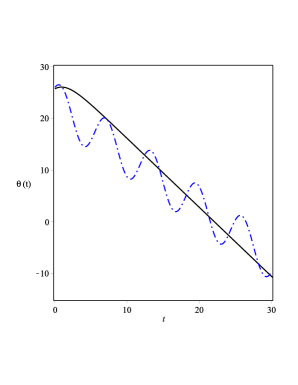
Figure 1: Qualitative behavior of the expansion scalar $\theta(t)$ as function of time for a typical choice of parameters for a beam of light which is initially diverging ($\theta(0)>0$). The solid black line shows the evolution for case 1 and blue dotted line for case 2. In both cases the effects of torsion causes $\theta(t)$ to vanish at some finite time and will be negative after that. If $\theta$ reaches $-\infty$ at some point along the beam trajectories, the beam starts converging after that time.

Remarkably the FRW torsion in the form of (32-33) does not change the shear tensor at all as the extra terms in the second term of R.H.S of (41) cancel out each other. By using equation (10) the evolution equation for the shear scalar $\sigma$ takes the form

$$\dot{\sigma}_{(0)}+2\theta_{(0)}\,\sigma_{(0)}=0$$ (45)

The vorticity changes as

$$\omega_{\alpha\beta}=\omega_{\alpha\beta(0)}-\frac{f(t)}{a(t)}$$ (46)

We are interested in the evolution of optical scalars. The equations (43) and (46) can be solved simultaneously to determine $\theta$ and $\sigma$. In reference DLP a modified form of the Frobenius’ theorem in the presence of torsion has been derived and it has been shown that in presence of torsion, hypersurface orthogonality of $k^{\mu}$ does not imply a vanishing vorticity tensor $\omega_{\alpha\beta}$ . However, in the special case of the homogenous and isotropic torsion (32-33) used here, the extra terms in eq. (B5) of reference DLP are canceled and one can set the vorticity to zero in this case. In order to solve the system of equations, the explicit form of the scale factor $a(t)$ and torsion function $h(t)$ are needed which one can get by solving the PGT field equations. The most general case involving seven unknown functions $q$, $s$, $h$ , $f$ , $\rho$ , $p$ and $a(t)$ is very complicated but there are several very interesting special cases which we will present here. For a full discussion of the solutions of the PGT field equations in various special cases see references Goen ; AQK ; Mink1 ; Mink2 ; Ao .

IV.1 Case 1

For an illustrative example we consider the solutions to the PGT field equations with zero spin density and axial torsion but non-vanishing vector torsion. In this case we set $f=s=q=0$ which represent reflection invariant solutions. The solution to the field equation also depends on the specific choice of coefficients $c_{1}-c_{5}$ in the Lagrangian (21) and also the value of $k$ in the metric (31). If $c_{1}+3c_{3}\neq 0$ then we have a solution with an effective cosmological constant in the form of $\Lambda=9c_{5}/(c_{1}+3c_{3})$. For the case of $\Lambda>0$ and $k=0$, the solutions are as follows

$$a(t)=a_{0}e^{\sqrt{\frac{\Lambda}{3}}t}$$ (47)

$$h(t)=\small{-\frac{\sqrt{3\Lambda}}{9}\frac{a(c\sqrt{3\Lambda}+3)e^{-c\sqrt{\frac{\Lambda}{3}}t}+b(d\sqrt{3\Lambda}+3)e^{-d\sqrt{\frac{\Lambda}{3}}t}}{ae^{-c\sqrt{\frac{\Lambda}{3}}t}+be^{-d\sqrt{\frac{\Lambda}{3}}t}}}$$ (48)

where $a$ and $b$ are constants of integration and $c$ and $d$ are some combination of coefficients. The solution for the scale factor in this case show a de Sitter expansion for the universe. Replacing this solutions to evolution equations for the optical scalars (42) and (45) and solving the system of equations, we find

$$\theta(t)=3a_{0}\sqrt{\frac{\Lambda}{3}}+\Bigg{[}(c+d+3)Ei\Bigg{(}1,\frac{(c+d+3)e^{-2\sqrt{\frac{\Lambda}{3}t}}}{2a^{2}_{0}}\Bigg{)}$$

$$+2\Lambda(c+d+3)^{3}e^{-2\sqrt{\frac{\Lambda}{3}t}}-2\Lambda(c+d+3)^{2}t$$

$$+\Big{(}27+4\Lambda(c+d+3)^{2}a^{2}_{0}\Big{)}e^{-\frac{1}{2}\frac{(c+d+3)^{3}}{a^{2}_{0}}e^{-2\sqrt{\frac{\Lambda}{3}t}}}\Bigg{]}$$

$$\times\Bigg{[}\sqrt{\Lambda}(2c+2d+6)\Bigg{]}^{-1}$$ (49)

Where $Ei(a,z)=z^{(a-1)}\Gamma(1-a,z)$ is the exponential integral. In the above relation, the first term on the R.H.S is the general relativistic result while all the other terms represent corrections due to the effects of torsion.

$$\sigma(t)=-\frac{21\Lambda}{16}(c+d+3)e^{-2\sqrt{\frac{\Lambda}{3}t}}+\frac{3}{70}Ei\Big{(}1,\frac{e^{-2\sqrt{\frac{\Lambda}{3}t}}}{4}\Big{)}$$

$$-\frac{(c+d+3)^{2}}{50}t^{2}+\frac{\sqrt{3\Lambda}}{32}\Bigg{(}t\,Ei\Big{(}1,\frac{1}{4}t\Big{)}-4e^{-\sqrt{\frac{3\Lambda}{4}}t}\Bigg{)}$$

The evolution of the expansion scalar $\theta$ in this case is shown in figure 1 for a typical choice of parameters (solid black line). We assumed that $\theta(0)>0$ which means that the beam is initially diverging. As one can see, $\theta$ will reach zero at some finite point in the affine parameter and will be negative after that. This means that the initially diverging beam will start converging at some point if $\theta$ reaches $-\infty$ at some finite affine parameter point along the trajectory of null geodesics. One can also find a relation for the angular diameter distance in this case by using relations (44) and (49).

IV.2 Case 2

For the specific case of $c_{1}=2$ and $c_{5}>0$ there is another possible interesting solution of PGT field equations as follows

$$a(t)=$$

$$\small{a_{0}\exp\Big{[}\frac{-\mu\,h_{0}\omega\,t+3H_{0}\omega\,t+\mu\,h_{0}\sin(\omega\,t)+3\alpha\,R_{0}\cos(\omega\,t)}{3\omega}\Big{]}}$$ (50)

and

$$h(t)=-\beta^{-1}R_{0}\sin(\omega\,t)+h_{0}\cos(\omega\,t)$$ (51)

where $\mu=c_{1}-c_{4}$, $\omega=\sqrt{\frac{2\mu}{c_{1}c_{5}}}$, $\alpha=\sqrt{\frac{c_{5}\mu}{72c_{1}}}$, $\beta=\sqrt{\frac{8\mu c_{1}}{c_{5}}}$ and $h_{0}$ and $H_{0}$ and $R_{0}$ are initial values of the torsion scalar $h$, the Hubble parameter and the curvature scalar respectively. In this case the optical scalars $\theta$ and $\sigma$ are given by solving the system of equations (42) and (45) as

$$\theta(t)=C_{1}e^{-t}$$

$$+\small{\Bigg{[}\Big{(}-18H_{0}\beta\,\omega^{2}-6\beta R_{0}\alpha\omega-2\beta h_{0}\mu+18R_{0}\omega\Big{)}\cos(\omega\,t)}$$

$$+\Big{(}18H_{0}\beta\,\omega-6\beta R_{0}\alpha-2\beta h_{0}\mu+18R_{0}\omega^{2}\Big{)}\sin(\omega\,t)$$

$$\small{+6\Big{(}\frac{1}{3}\mu h_{0}-H_{0}-\frac{1}{2}\Big{)}(1+\omega^{2})\beta\Bigg{]}\times\Bigg{[}6\beta(\omega^{2}+1)\Bigg{]}^{-1}}$$ (52)

the shear scalar in this case then is given by

$$\sigma(t)=C_{2}e^{\int\frac{\theta(t)a(t)}{C_{3}}dt}$$ (53)

where $C_{1-3}$ again are constants of integration. The behavior of the expansion scalar in this case is also depicted in figure 2 by the blue dotted line. Similar to case 1, the expansion scalar for an initially diverging beam reaches zero at some point along the ray trajectories and will be negative after that.

Let us now briefly discuss how the presence of torsion modify the evolution of the polarization vector defined in (37). It is a well known fact that in general relativity, the polarization vector is parallel transported along the trajectory of light rays. However it has been shown that in a spacetime with torsion this will not be the case in general Ritis . The Maxwell’s wave equation in the presence of torsion reads Ritis ; Pras

$$\nabla_{\nu}\nabla^{\nu}A^{\mu}-(2T^{\mu\nu\rho}+Q^{\mu\nu\rho})(\nabla_{\nu}A_{\rho}-\nabla_{\nu}A_{\rho})$$

$$-(2\nabla_{\nu}T_{~{}~{}\rho}^{\mu\nu}+2\nabla_{\nu}Q_{~{}~{}\rho}^{\mu\nu}+R_{~{}~{}\rho}^{\mu})A\rho=0$$ (54)

where

$$Q^{~{}~{}\rho}_{\mu\nu}\equiv T^{~{}~{}\rho}_{\mu\nu}+\delta^{\rho}_{\mu}T^{~{}~{}\sigma}_{\nu\sigma}-\delta^{\rho}_{\nu}T^{~{}~{}\sigma}_{\mu\sigma}$$ (55)

Using equation (37) we get the following equation for the evolution of the polarization vector

$$k^{\nu}\nabla_{\nu}\epsilon^{\mu}=\frac{1}{2}\epsilon^{\mu}\Big{[}(2T^{\rho\nu\sigma}+Q^{\sigma\nu\rho})(\epsilon_{\rho}^{*}k_{[\sigma}\epsilon_{\nu]}+\epsilon_{\rho}k_{[\sigma}\epsilon^{~{}~{}*}_{\nu]})$$

$$-\frac{1}{2}(2T^{\rho\nu\sigma}+Q^{\sigma\nu\rho})(k_{\sigma}\epsilon_{\nu}+k_{\sigma}\epsilon_{\nu})\Big{]}$$ (56)

substituting for torsion in the FRW background from equation (32) and (33) we see that the polarization vector is not parallel transported along the light ray trajectories.

V Conclusion and discussion

Geometric optics and the evolution of the optical scalars have found many interesting cosmological applications over the years. Any slight deviation from the general relativistic equations governing the light propagation, may have far reaching consequences in many areas of astrophysics and cosmology. For example, number and location of images from cosmological gravitational lenses, development of caustics, measurement of the angular diameter distance for cosmological objects and also study of the CMB spectrum are all directly dependent on the light propagation equations and the properties of the bundle of light rays. In Poincaré gauge theory of gravity, the gravitational interaction is described not only by curvature, but also by the torsion of spacetime. Torsion is also present in many other approaches to gravity such as string theory GSW , supergravity PT and theories involving twistors Pap . It has been shown that the presence of torsion will modify the Raychaudhuri equation for the expansion scalar and also equations governing the evolution of shear and vorticity tensors. Here, we derive the explicit form of the expansion and shear for a homogeneous and isotropic FRW background in the Poincaré gauge theory of gravity. We also solved the evolution equations for optical scalars and found the analytical solutions for two different cases in PGT. The result shows that in general, the evolution of optical scalars in a cosmological background will be different in spacetimes with torsion and in general relativity. This may provide an indirect test of torsion theories by carefully studying gravitational lensing and other similar effects.

References

- (1) A. K. Raychaudhuri, Phys. Rev. 98, 1123 (1955).
- (2) R. Penrose, Phys. Rev. Lett. 14, 57 (1965).
- (3) S. W. Hawking, Phys. Rev. Lett. 15, 689 (1965); Phys. Rev. Lett. 17, 444 (1966).
- (4) R. K. Sachs, Proc. Roy. Soc. (London) A 264, 309 (1961).
- (5) S. Hawking and G. F. R. Ellis, The Large Scale Structure of Space-Time (Cambridge University Press, Cambridge, 1973).
- (6) R.M. Wald, General Relativity, University of Chicago Press, Chicago U.S.A. (1984).
- (7) M. Sasaki, Prog. Theor. Phys. 90 (1993) 753.
- (8) P. Schneider, J. Ehlers and E.E. Falco, Gravitational Lenses, Springer-Verlag, New York U.S.A. (1992).
- (9) D. Puetzfeld and Y. N. Obukhov, Phys. Rev. D 76, 084025 (2007) Erratum: [Phys. Rev. D 79, 069902 (2009)].
- (10) P. B. Yasskin and W. R. Stoeger, Phys. Rev. D 21, 2081 (1980).
- (11) K. Nomura, T. Shirafuji and K. Hayashi, Prog. Theor. Phys. 87, 1275 (1992).
- (12) S. Capozziello, G. Lambiase , C. Stornaiolo, Ann. der Phys. 10, 713 (2001).
- (13) M. Blagojevic, Gravitation and Gauge Symmetries (IoP Publishing, Bristol, 2002).
- (14) K. Hayashi and T. Shirafuji, Prog. Theor. Phys. 64, 866 (1980); 64, 883 (1980); 64, 1435 (1980); 64, 2222 (1980); 65, 525 (1981); 66, 318 (1981); 66, 2258 (1981).
- (15) F. W. Hehl, P. von der Heyde, and G. D. Kerlick Phys. Rev. D 10, 1066 (1974).
- (16) R. Rauch, Phys. Rev. D26, 931 (1982).
- (17) M. Blagojevi c and F. W. Hehl (eds.), Gauge Theories of Gravitation. A Reader with Commentaries (Imperial College Press, London, 2013).
- (18) E. Poisson, A relativist s toolkit: the mathematics of black hole mechanics, (Cambridge University Press, Cambridge, UK, 2004).
- (19) M. I. Wanas and M. A. Bakry, Int. J. Mod. Phys. A 24, 5025 (2009).
- (20) S. Kar and S. Sengupta, Pramana 69, 49 (2007).
- (21) P. Luz and V. Vitagliano, Phys. Rev. D96 no.2, 024021 (2017).
- (22) K.-F. Shie, J. M. Nester, and H.-J. Yo, Phys. Rev. D 78, 023522 (2008).
- (23) M. Tsamparlis, Phys. Lett. A 75, 27 2 (1979).
- (24) G.G.A. Bauerle and CHR.J. Hanveld, Physica 12lA, 541-551(1983).
- (25) H. Goenner and F. M uller-Hoissen, Class. Quantum Grav. 1, 651 672 (1984).
- (26) V. I Kudin, A. V Minkevich and F. I Fedorov, Vesci Akad. Nauuk BSSR. Ser. Fiz.-Mat. Nauuk 4 59 ( 1981).
- (27) M. Gasperini, Phys. Rev. Lett. 56, 2873-2876 (1986).
- (28) I. S. Nurgaliev and V. N. Ponomariev, Phys. Lett. 1308, 378 (1983).
- (29) C. W. Misner, K.S. Thorne and J. A. Wheeler, Gravitation, W.H. Freeman and Company, New York U.S.A. (1973).
- (30) R. Dey, S. Liberati and D. Pranzetti, Phys. Rev. D 96, 124032 (2017)
- (31) S. Akhshabi, E. Ghorani and F. Khajenabi, EPL, 119 29002 (2017).
- (32) A.V Minkevich, Class. Quantum Grav. 23, 4237 (2006) ; Mod. Phys. Lett. A26, 259(2011); Int. J. Mod. Phys. A31 1641011, (2016).
- (33) A.V Minkevich, Class. Quantum Grav. 24, 5835 (2007); Phys. Lett. B678, 423 (2009).
- (34) X.-C. Ao, X.-Z. Li, and P. Xi, Phys. Lett. B694 186 190 (2010).
- (35) R. de Ritis, M. Lavorgna, C. Stornaiolo, Phys.Lett. 98A, 411 (1983).
- (36) A. R. Prasanna, Phys. Lett. 54A , 17 (1975).
- (37) M.B. Green, J.H. Schwarz, E. Witten, Superstring Theory, (Cambridge University Press, Cambridge, UK, 1987).
- (38) G. Papadopoulos, P.K. Townsend, Nucl. Phys. B444, 245 (1995).
- (39) G. Papadopoulos, Phys. Lett. 379B, 80 (1996).