Migration of Planets Into and Out of Mean Motion Resonances in Protoplanetary Discs: Overstability of Capture and Nonlinear Eccentricity Damping

Abstract

A number of multiplanet systems are observed to contain planets very close to mean motion resonances, although there is no significant pileup of precise resonance pairs. We present theoretical and numerical studies on the outcome of capture into first-order mean motion resonances (MMRs) using a parametrized planet migration model that takes into account nonlinear eccentricity damping due to planet-disk interaction. This parametrization is based on numerical hydrodynamical simulations and is more realistic than the simple linear parametrization widely used in previous analytic studies. We find that nonlinear eccentricity damping can significantly influence the stability and outcome of resonance capture. In particular, the equilibrium eccentricity of the planet captured into MMRs become larger, and the captured MMR state tends to be more stable compared to the prediction based on the simple migration model. In addition, when the migration is sufficiently fast or/and the planet mass ratio is sufficiently small, we observe a novel phenomenon of eccentricity overshoot, where the planet’s eccentricity becomes very large before settling down to the lower equilibrium value. This can lead to the ejection of the smaller planet if its eccentricity approaches unity during the overshoot. This may help explain the lack of low-mass planet companion of hot Jupiters when compared to warm Jupiters.

1 Introduction

The Kepler mission has discovered thousands of exoplanets, many of which are in multi-planet systems (Batalha et al., 2013; Coughlin et al., 2016). The period ratio distribution of the Kepler planets shows a significant excess of planet pairs with period ratio near mean motion resonances (MMRs) (Fabrycky et al., 2014). This excess of planets near (or in) MMRs, together with the discovery of several resonant chain systems, such as Kepler-223 (Mills et al., 2016) and TRAPPIST-1 (Luger et al., 2017), suggests that resonance capture during disk-driven migration can be common. However, the MMR capture rate predicted using a relatively “clean” migration model is much higher than the observed occurrence rate of MMRs. This discrepancy is often explained by the disruption of MMRs by physical processes after the resonance capture, including instability of the captured state during disk-driven migration (Goldreich & Schlichting, 2014; Deck & Batygin, 2015; Delisle et al., 2015; Xu & Lai, 2017), tidal dissipation in planets (Lithwick & Wu, 2012; Batygin & Morbidelli, 2013; Delisle et al., 2014), late time dynamical instability (Pu & Wu, 2015; Izidoro et al., 2017), and outward (divergent) migration due to planetesimal scattering (Chatterjee & Ford, 2015). Regardless of whether MMRs are maintained or destroyed by any of these processes, it is important to recognize that MMRs, even if temporarily maintained, play a significant role in the early evolution of planetary systems and can profoundly shape their final architectures.

A majority of the studies on the outcome of MMR capture (such as the impact of MMR on the orbital parameters of the planets and the stability of the resonance) include the effect of disk-driven migration using a simple parametrized migration model, the most commonly used being that given by Goldreich & Tremaine (1980). The choice of this parametrized migration model makes the equation of motion of the system relatively simple, which is ideal for long-term numerical integrations or analytical studies. However, this model only works well for small eccentricities ($e\lesssim H/r$, the aspect ratio of the disk). As we show in this paper, the eccentricities of the planets near MMR can often lie in the regime where the Goldreich & Tremaine (1980) result is no longer valid. This can impact the outcome of the resonance capture. There are also a number of studies that includes more realistic migration models, such as those using parametrized forcing in $N$-body integration (e.g. Terquem & Papaloizou 2007; Migaszewski 2015) or using self-consistent hydrodynamics (e.g. Kley et al. 2005; Papaloizou & Szuszkiewicz 2005; Crida et al. 2008; Zhang et al. 2014; André & Papaloizou 2016). However, these studies tend to focus on explaining the behaviors of particular systems and do not survey a sufficiently large parameter space to obtain various possible outcomes. The goal of our paper is to remedy this situation. In particular, we generalize previous analyses (Goldreich & Schlichting, 2014; Deck & Batygin, 2015; Delisle et al., 2015; Xu & Lai, 2017) by adopting a more realistic parametrization for the migration and eccentricity damping, and examine how different model parameters affect the outcome of the MMR capture.

This paper is organized as follows. Section 2 summarizes the parametrizations for the rates of orbit decay and eccentricity damping due to planet-disk interactions. In Section 3 we consider the simple case when one of the planets is massless and study how different parametrizations can affect the outcome of MMR capture. We find that using the more realistic migration model can sometimes cause the ejection of the small planet, but otherwise tend to increase the stability of the resonance. In Section 4 we study the more realistic case when both planets have finite masses. While most of the results from Section 3 can be generalized, we also observe several new phenomena that arise only when both planets have finite masses. In addition to analytical calculations, we use 3-body integrations to validate our results. We conclude in Section 5 and discuss how our results affect the architecture of multi-planet systems.

2 Parametrizations of the rates of orbit decay and eccentricity damping

Consider a small planet undergoing type I migration in a gaseous disk. At low eccentricity, the rates of orbit decay and eccentricity damping due to planet-disk interaction are approximately given by (Goldreich & Tremaine, 1980)

$$\frac{\dot{a}}{a}=-\frac{1}{T_{m}}-\frac{2pe^{2}}{T_{e}},$$ (1)

$$\frac{\dot{e}}{e}=-\frac{1}{T_{e}},$$ (2)

where $T_{m},T_{e}$ are independent of $e$ and $T_{m}\sim T_{e}h^{-2}$, with $h\equiv H(r)/r$ ($H$ is the disk’s scale height). The parameter $p$ characterizes the coupling between orbit decay and eccentricity damping; here we take $p=1$, which corresponds to eccentricity damping that conserves angular momentum. This is the parametrized migration model used in most studies of MMR capture (Goldreich & Schlichting, 2014; Deck & Batygin, 2015; Delisle et al., 2015; Xu & Lai, 2017).

However, this migration model is accurate only for small eccentricities, $e\lesssim h$. For larger eccentricities, hydrodynamic simulations (Cresswell et al., 2007; Cresswell & Nelson, 2008) show that the orbit decay rate and eccentricity damping rate both decrease. As an empirical fit to the numerical results, $T_{m}$ and $T_{e}$ are functions of $e/h$ given by (based on Eqs. 11 and 13 of Cresswell & Nelson 2008)

$$T_{m}=T_{m,0}\frac{1+(e/2.25h)^{1.2}+(e/2.84h)^{6}}{1-(e/2.02h)^{4}},$$ (3)

$$T_{e}=T_{e,0}\left(1-0.14\frac{e^{2}}{h^{2}}+0.06\frac{e^{3}}{h^{3}}\right),$$ (4)

$${\rm with~{}~{}}T_{m,0}\equiv\frac{t_{\rm wave}}{2.7+1.1\beta}h^{-2},~{}~{}T_{e,0}\equiv\frac{t_{\rm wave}}{0.78}.$$ (5)

Here we assume that the disk has a density profile $\Sigma(r)\propto r^{-\beta}$; we adopt $\beta=0$ (i.e. a disk with uniform surface density) unless otherwise specified. The timescale $t_{\rm wave}$ is given by (Takana & Ward 2004)

$$\begin{split}t_{\rm wave}=\frac{M_{\star}^{2}}{\Sigma a^{2}m}h^{4}\Omega^{-1},\end{split}$$ (6)

with $\Omega$ being the angular velocity of the unperturbed disk.

In this paper we compare two different migration models/ parametrizations: the “simple” model, with $T_{m}=T_{m,0}$ and $T_{e}=T_{e,0}$ independent of $e$, and the “realistic” model, with $T_{m},T_{e}$ given by equations (3) and (4). The two models are identical for $e/h\ll 1$, but can give very different orbit decay and eccentricity damping rates when $e/h$ is large. This is illustrated in Figure 1. In particular, for the realistic migration model, the eccentricity damping rate scales as $e^{-3}$ when $e/h\gg 1$.

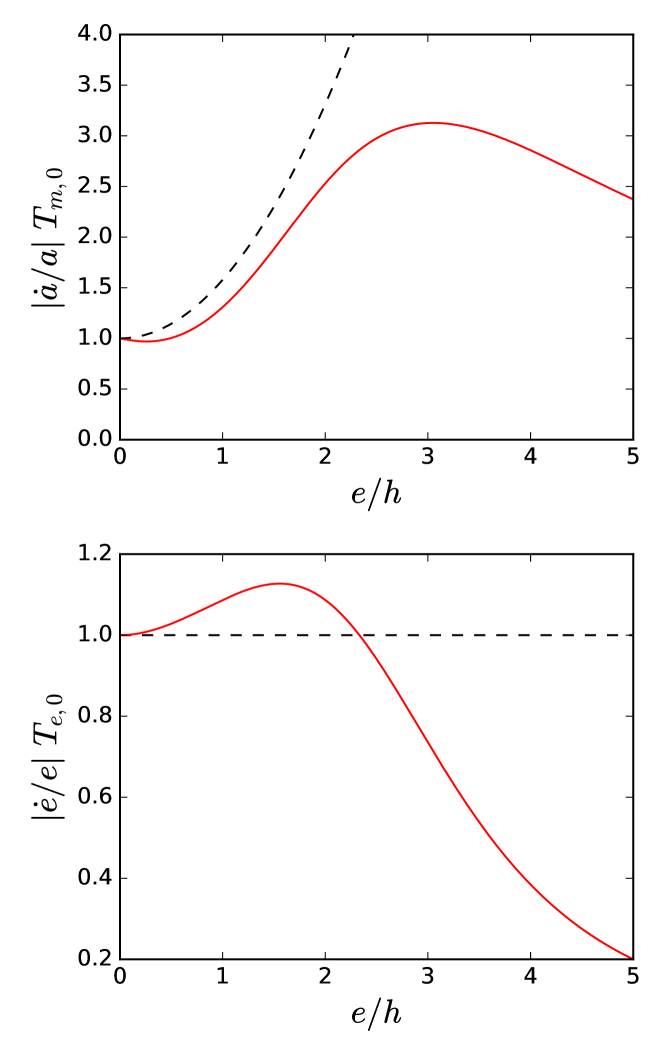
Figure 1: Orbit decay and eccentricity damping rates given by the simple migration model (eccentricity-independent $T_{e},T_{m}$, black dashed curves) and the realistic migration model (eccentricity-dependent $T_{e},T_{m}$, red solid curves). The difference becomes prominent when $e/h\gtrsim 3$.

3 Outcome of MMR capture: massless inner planet

To gain some analytical understanding to the general problem of MMR capture with comparable mass planets, in this section we consider a simpler case: a planet with negligible mass ($m$) perturbed by an outer massive planet ($m^{\prime}$) on a circular orbit near a first-order $j:j+1$ MMR. To this end, we take $T_{m}^{\prime}$, the orbit decay timescale of the outer planet, to be a free parameter. This allows us to explore how the equilibrium eccentricity (of the inner planet), which is determined by the net convergent migration rate, affects the outcome of the MMR capture. In reality, both planets undergo migration. For $m\ll m^{\prime}$ and Type I migration, we expect $T_{m},T_{e}h^{-2}\gg T_{m}^{\prime}$. The results in this section should qualitatively illustrate how the outcomes of MMR capture are affected when the realistic migration model is applied (see Section 4).

In this section, we also assume that the planet-disk interaction is weak, so that $T_{m},T_{e},T_{m}^{\prime}$ (note that $T_{e}^{\prime}$ is irrelevant since the outer planet’s orbit is always circular) are much greater than the timescale of libration, $T_{\rm res}$, given by

$$\begin{split}T_{\rm res}\approx 0.8j^{-4/3}(\mu^{\prime})^{-2/3}\frac{2\pi}{n},\end{split}$$ (7)

where $n$ is the mean motion of the inner planet and $\mu^{\prime}=m^{\prime}/M_{\star}$ the mass ratio between the outer planet and the star. (For the exact definition of $T_{\rm res}$, see Eq. B6 in Appendix B of Xu & Lai 2017.) For simplicity, we assume that $T_{e,0},T_{m,0},T_{m}^{\prime}$ remain constant (i.e. their variations due to the evolution of the planets’ semi-major axes are ignored).

3.1 Existence of equilibrium

We first study the eccentricity at the equilibrium state (and whether such equilibrium state exists). Near a first-order $j:j+1$ MMR, the resonant motion conserves

$$\begin{split}\alpha_{0}\equiv\alpha(1+je^{2}),\end{split}$$ (8)

where $\alpha=a/a^{\prime}<1$ is the semi-major axis ratio. When the system undergoes convergent migration, the inner planet can be captured into the resonance. It reaches an equilibrium state when $d\alpha_{0}/dt=0$, which corresponds to

$$\begin{split}T_{m,\rm eff}^{-1}=2(j+1)e^{2}T_{e}^{-1}.\end{split}$$ (9)

Here $T_{m,\rm eff}$ (which may depend on $e$) is the effective convergent migration rate given by $T_{m,\rm eff}^{-1}\equiv T_{m}^{\prime-1}-T_{m}^{-1}$. Note that when the outer planet is much more massive it should migrate much faster than the inner planet, so $T_{m,\rm eff}\approx T_{m}^{\prime}$.

For the simple migration model with constant $T_{e}=T_{e,0}$ and $T_{m}=T_{m,0}$, the equilibrium always exists, with the corresponding eccentricity given by (Goldreich & Schlichting, 2014)

$$\begin{split}e_{\rm eq,0}=\sqrt{\frac{T_{e,0}}{2(j+1)T_{m,\rm eff,0}}}\simeq\sqrt{\frac{T_{e,0}}{2(j+1)T_{m}^{\prime}}},\end{split}$$ (10)

where $T_{m,\rm eff,0}^{-1}\equiv T_{m}^{\prime-1}-T_{m,0}^{-1}$.

However, for the realistic migration model with eccentricity-dependent $T_{e}$ and $T_{m}$, the right-hand side of (9) has a finite maximum value because for $e\gtrsim$ a few $h$, $e^{2}T_{e}^{-1}\propto e^{-1}$ decreases as $e$ increases. Therefore, the equilibrium may not exist when the outer planet’s migration is too fast. The maximum value of $e^{2}T_{e}^{-1}$ occurs at $e\simeq 3h$, thus the equilibrium ceases to exist when

$$\begin{split}T_{m}^{\prime-1}\gtrsim 2(j+1)T_{e,0}^{-1}(3h)^{2}.\end{split}$$ (11)

Figure 2 gives an example of the evolution of the system when the equilibrium of resonance capture does not exist.

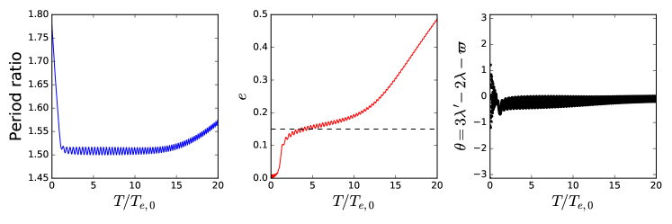
Figure 2: Evolution of a system near 2:3 MMR with $h=0.05$, $T_{m}^{\prime}=10T_{e,0}$, and the outer planet mass $\mu^{\prime}=m^{\prime}/M_{\star}=10^{-3}$. Left panel: period ratio. Center panel: eccentricity of the inner planet. The black dashed line shows $e=3h$ for reference. Right panel: resonant angle. The equilibrium does not exist and the planet’s eccentricity grows unboundedly as the system goes deeper into the resonance. This increasing eccentricity should ultimately cause ejection or collision of the planet.

3.2 Stability of capture

The migration model can also affect the stability of the captured (equilibrium) state.

For the simple migration model, the stability of the equilibrium state has been studied by Goldreich & Schlichting (2014). Under the assumption that planet-disk interaction is weak, the behavior of the system depends only on the ratio $\mu^{\prime}/e_{\rm eq,0}^{3}$, where $\mu^{\prime}=m^{\prime}/M_{\star}$ and $e_{\rm eq,0}$ is the previously defined equilibrium eccentricity. The equilibrium is stable when the outer planet is sufficiently massive (with $\mu^{\prime}\gtrsim e_{\rm eq,0}^{3}$); in this case the resonant angle librates with small amplitude. For $\mu^{\prime}\sim e_{\rm eq,0}^{3}$, the libration amplitude saturates at a finite value, and the system stays in resonance. For a less massive outer planet (with $\mu^{\prime}\lesssim e_{\rm eq,0}^{3}$), the equilibrium state is overstable (i.e. the amplitude of libration increases with time) and the system eventually escapes from resonance.

For the realistic migration model, however, the stability of the equilibrium state depends on not only $\mu^{\prime}/e_{eq,0}^{3}$ but also $e_{\rm eq,0}/h$; the latter parameter characterizes how significantly the system is affected by including the eccentricity dependence in the migration model.

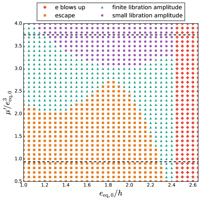
Figure 3: Regimes of different behaviors in the $e_{eq,0}/h$ - $\mu^{\prime}/e_{eq,0}^{3}$ parameter space for a 2:3 MMR. The two dashed lines mark the analytical estimates for the boundary between libration with small amplitude, libration with finite amplitude and escape given by Goldreich & Schlichting (2014) for the simple migration model.

Figure 3 plots the regimes of different behaviors in the $e_{eq,0}/h$ - $\mu^{\prime}/e_{eq,0}^{3}$ parameter space for a 2:3 MMR when the realistic migration model is applied. We integrate the equation of motion derived from the resonance Hamiltonian (see, e.g., Appendix B of Xu & Lai 2017), and include the dissipative terms associated with migration and eccentricity damping. We find that there are four possible outcomes/behaviors:

(i) When $e_{eq,0}$ is larger than $2.4h$, the equilibrium state of resonance capture does not exist because the eccentricity damping is too weak to balance the eccentricity excitation due to resonant interaction, and the planet’s eccentricity $e$ grows unboundedly until the system becomes unstable (red diamonds in Fig. 3).

(ii)-(iv) When $e_{eq,0}$ is small enough to allow the existence of an equilibrium state, this equilibrium can be stable or overstable. When it is stable, the system exhibits small libration around the equilibrium state with the libration amplitude converging to zero (purple circles in Fig. 3). When it is overstable, the system can either end up in a stable state with a finite libration amplitude (green triangles) or exit the resonance with damped eccentricity (orange squares). Only these three behaviors are possible in the simple migration model.

Although Figure 3 refers to the 2:3 MMR, we find that the results for other first-order MMRs are qualitatively similar.

Three-body simulations (see below) show that the results obtained from the resonant Hamiltonian in Figure 3 are qualitatively correct, with tolerable error for the boundaries between different behaviors. Note that the boundaries between the last three behaviors (stable libration with finite and small amplitude, and escape) depend sensitively on the migration model, since the stability of the equilibrium is affected by the derivatives of $T_{e}$ and $T_{m}$.

Figure 3 differs from the result based on the simple migration model (e.g. Goldreich & Schlichting 2014) in several aspects. First, as noted above, there exists a new regime where the planet’s eccentricity can grow unboundedly because of the decrease of eccentricity damping rate for $e\gtrsim h$. Second, near the boundary of this “eccentricity blowing up” regime ($2.3\lesssim e_{eq,0}/h\lesssim 2.45$), the stable finite-amplitude libration regime occupies a large parameter space; in particular, the system can stay in resonance with a finite-amplitude libration even when $\mu^{\prime}/e_{eq,0}^{3}$ is as small as $0.6$ (by contrast, the simple migration model would predict the system escape from the resonance due to overstability). Third, the boundaries between the different regimes, even at $e_{eq,0}/h\lesssim 2$ (for which $T_{m}$ and $T_{e}$ deviate little from the simple model), are significantly distorted due to the use of the more realistic migration model, showing that these boundaries are indeed sensitive to the migration model (and disk parameters). Note that for low eccentricity ($e_{\rm eq,0}/h\lesssim 1$) our result may not be accurate given that the fitting used to obtain equations (3) and (4) may introduce nontrivial error in the derivatives of $T_{m}$ and $T_{e}$ when $e\to 0$. Therefore, we do not expect our model to recover the analytical result of Goldreich & Schlichting (2014) for small $e_{\rm eq}$, and result for $e_{\rm eq}/h<1$ is not shown in Figure 3.

Figures 4-7 show the behavior of the system in each regime depicted in Fig. 3. These results are obtained by doing 3-body integrations using the MERCURY code (Chambers, 1999), with $h=0.025$, $a^{\prime}=1$ au and $T_{e,0}=10T_{\rm res}$ [with $T_{\rm res}$ given by equation (7)]. The other parameters of the system can be solved to match the given $e_{eq,0}/h$ and $\mu^{\prime}/e_{eq,0}^{3}$ values. In practice, to avoid having the planets migrate too far inward during the integration (which will make it necessary to choose a much smaller timestep to account for the planet’s short orbital period), we fix the outer planet and let the inner planet’s semi-major axis increase at the rate $\dot{a}/a=-1/T_{m}-2e^{2}/T_{e}+1/T_{m}^{\prime}$ — Note that this parameterized treatment is necessary because the overstability timescale of the equilibrium state can be $\gtrsim 10T_{m}^{\prime}$ in many cases.

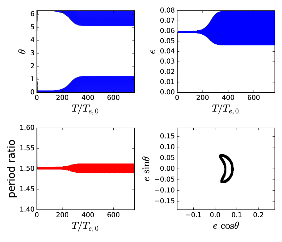
Figure 4: Evolution of a system captured into the 2:3 MMR with $e_{{\rm eq},0}/h=2.3$ and $\mu^{\prime}/e_{{\rm eq},0}^{3}=1$. The four panels plot the inner planet’s resonant angle, eccentricity, the two planet’s period ratio, and the inner planet’s trajectory in $e\cos\theta$ - $e\sin\theta$ phase space after reaching the equilibrium. The system ends up in a stable state with finite libration amplitude.

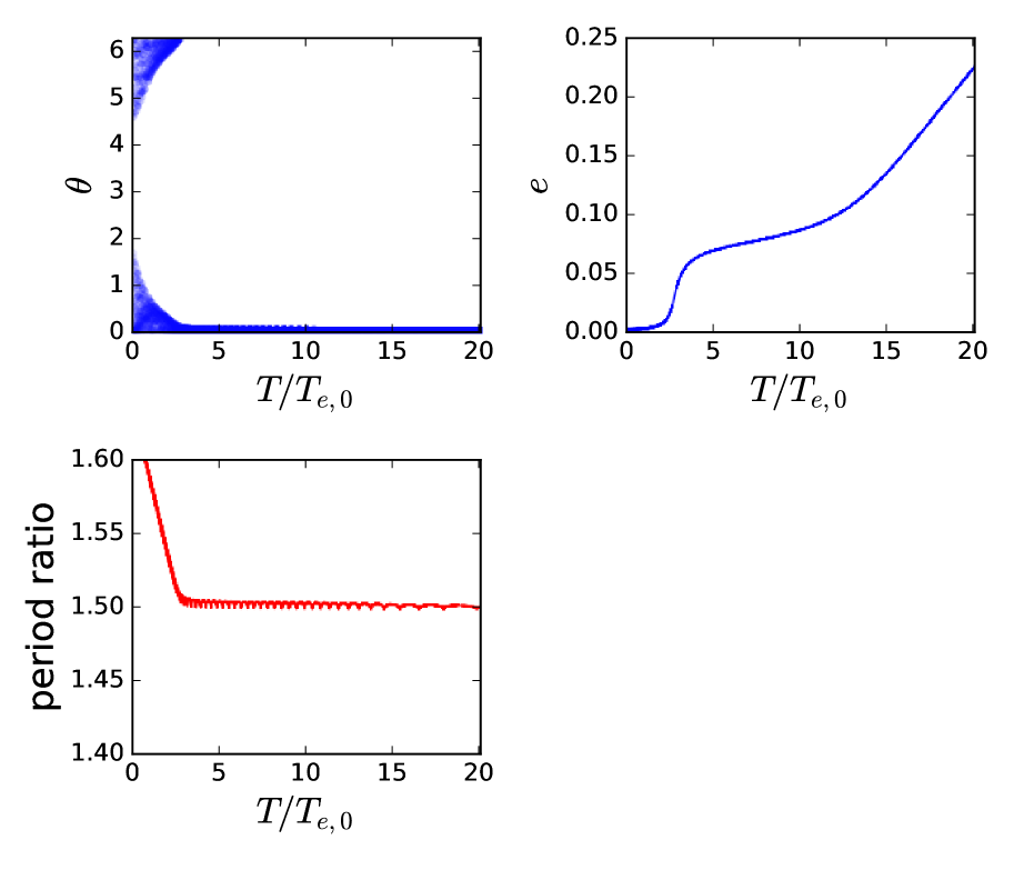
Figure 5: Same as Fig. 4, but with $e_{{\rm eq},0}/h=2.5$ and $\mu^{\prime}/e_{{\rm eq},0}^{3}=1$. Equilibrium no longer exists and the planet’s eccentricity grows unboundedly. The system eventually becomes unstable and the inner planet gets ejected shortly after $e$ reaches $\sim 0.8$.

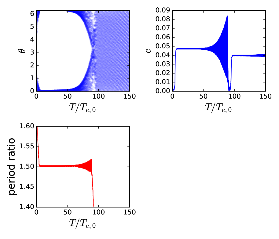
Figure 6: Same as Fig. 4, but with $e_{{\rm eq},0}/h=2$ and $\mu^{\prime}/e_{{\rm eq},0}^{3}=1$. The planet escapes from the resonance due to the overstability of the equilibrium state. Note that soon after the planet exits the 2:3 MMR, it gets captured into a 3:4 MMR.

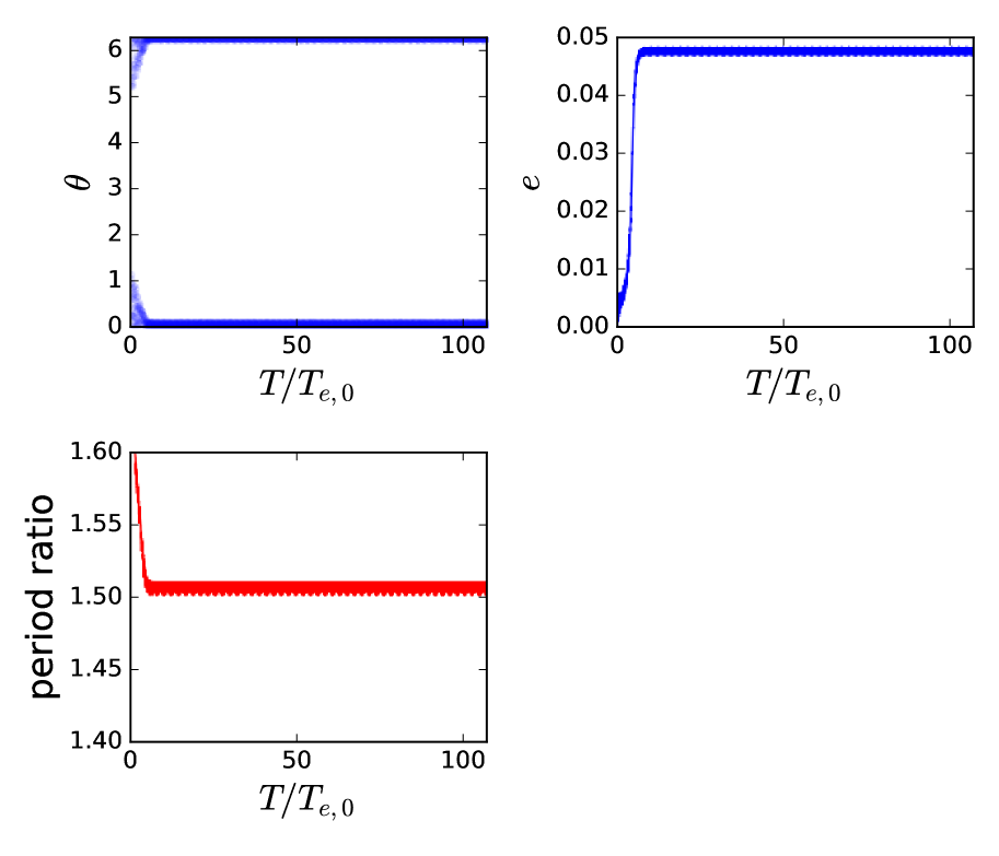
Figure 7: Same as Fig. 4, but with $e_{{\rm eq},0}/h=2$ and $\mu^{\prime}/e_{{\rm eq},0}^{3}=3.5$. The equilibrium state is stable and the libration of the resonant angle stays small.

4 Outcome of MMR capture: two massive planets

To apply our results to realistic systems, it is important to study the case where both planets have finite masses. As we will show in this section, the perturbation on the more massive planet from the smaller planet can qualitatively affect the outcome of resonance capture even when the mass ratio is very small. We will also discuss the effect of strong eccentricity damping rate and non-adiabatic evolution due to fast migration.

4.1 Existence and location of equilibrium

Consider two planets near a $j:j+1$ MMR, with both planets having finite masses. Let the inner (outer) planet have mass $m_{1}$ ($m_{2}$) and semi-major axis $a_{1}$ ($a_{2}$). The Hamiltonian of the system, to first order in eccentricity and with all non-resonant terms averaged out, is given by

$$\begin{split}H=&-\frac{GM_{\star}m_{1}}{2a_{1}}-\frac{GM_{\star}m_{2}}{2a_{2}}\\ &-\frac{Gm_{1}m_{2}}{a_{2}}\left(f_{j+1,27}\,e_{1}\cos\theta_{1}+\tilde{f}_{j+1,31}\,e_{2}\cos\theta_{2}\right).\end{split}$$ (12)

Here $\alpha=a_{1}/a_{2}$, and $f_{m,n}$ are functions of $\alpha$ (evaluated at $\alpha_{0}\equiv[j/(j+1)]^{2/3}$) given in Appendix B of Murray & Dermott (1999), with $\tilde{f}_{j+1,31}\equiv f_{j+1,31}-\delta_{j,1}2\alpha_{0}$. The interaction between the two planets conserves the total angular momentum

$$\begin{split}\mathcal{L}\equiv\Lambda_{1}\sqrt{1-e_{1}^{2}}+\Lambda_{2}\sqrt{1-e_{2}^{2}},\end{split}$$ (13)

where $\Lambda_{i}=m_{i}\sqrt{GM_{\star}a_{i}}$. The Hamiltonian (12) also admits a second constant of motion (Michtchenko & Ferraz-Mello, 2001),

$$\begin{split}\mathcal{K}\equiv\frac{j+1}{j}\Lambda_{1}+\Lambda_{2}.\end{split}$$ (14)

Combining the two ($\mathcal{L}$ and $\mathcal{K}$) produces a conserved quantity $\eta$, given by

$$\begin{split}\eta&\equiv-2(q\alpha_{0}^{-1}+1)\left[\frac{\mathcal{L}}{\mathcal{K}}-\left(\frac{\mathcal{L}}{\mathcal{K}}\right)_{\alpha=\alpha_{0},e_{i}=0}\right]\\ &\approx\frac{q}{j\alpha_{0}^{1/2}(q\alpha_{0}^{-1}+1)}(\alpha-\alpha_{0})+\alpha_{0}^{1/2}qe_{1}^{2}+e_{2}^{2},\end{split}$$ (15)

where $q=m_{1}/m_{2}$ is the mass ratio, and $\alpha_{0}=[j/(j+1)]^{2/3}$ is the semi-major axis ratio at resonance. In the second line of equation (15) we have expanded the result to the lowest order in $(\alpha-\alpha_{0})$ and $e_{i}^{2}$. The parameter $\eta$ characterizes how deep the system is inside the resonance when captured: For larger $\eta$, the system is deeper inside the resonance, and the fixed point (libration center) of the system corresponds to larger eccentricities.

Consider the evolution of $e_{i},\varpi_{1}-\varpi_{2}$ and $\eta$. At the equilibrium state, $\varpi_{1}-\varpi_{2}$ is constant because the resonant angles $\theta_{i}\equiv(j+1)\lambda_{2}-j\lambda_{1}-\varpi_{i}$ are constant; $\eta$, which is a function of $\alpha$ and $e_{i}$, should also be constant because $\alpha,e_{i}$ are constant. Therefore, $e_{i}$ and $\theta_{i}$ at the equilibrium state can be solved from the following equations:

$$\frac{de_{1}}{dt}=-\mu_{2}n_{1}\alpha_{0}f_{j+1,27}\sin\theta_{1}-\frac{e_{1}}{T_{e,1}}=0,$$ (16)

$$\frac{de_{2}}{dt}=-\mu_{1}n_{2}\tilde{f}_{j+1,31}\sin\theta_{2}-\frac{e_{2}}{T_{e,2}}=0,$$ (17)

$$\frac{d(\varpi_{1}-\varpi_{2})}{dt}\propto f_{j+1,27}e_{2}\cos\theta_{1}-\tilde{f}_{j+1,37}e_{1}q\alpha_{0}^{1/2}\cos\theta_{2}=0,$$ (18)

$$\frac{d\eta}{dt}=\frac{q\alpha_{0}^{1/2}}{j(q\alpha_{0}^{-1}+1)}\left(\frac{1}{T_{m,2}}-\frac{1}{T_{m,1}}+\frac{2e_{1}^{2}}{T_{e,1}}-\frac{2e_{2}^{2}}{T_{e,2}}\right)$$

$$~{}~{}~{}~{}~{}~{}~{}~{}-q\alpha_{0}^{1/2}\frac{2e_{1}^{2}}{T_{e,1}}-\frac{2e_{2}^{2}}{T_{e,2}}=0.$$ (19)

Note that since $\eta$ is conserved in the absence of dissipation (planet-disk interaction), equation (19) only includes contributions from planet-disk interactions. Equation (19) can be interpreted physically as that convergent migration tends to push the system deeper into resonance (i.e. increases $\eta$ and eccentricities) and while eccentricity damping (from planet-disk interaction) counters the effect of migration. Equilibrium is reached ($\eta$ ceases to evolve) when migration and eccentricity damping balance each other.

4.1.1 Weak eccentricity damping

First consider the case when the eccentricity damping is weak, i.e. $\mu_{2}n_{1}\gg e_{1}/T_{e,1}$ and $\mu_{1}n_{2}\gg e_{2}/T_{e,2}$. In this case, $|\cos\theta_{i}|\approx 1$, and equation (18) gives $e_{1}/e_{2}$ at the equilibrium. Note that $e_{1}/e_{2}\sim q^{-1}=m_{2}/m_{1}$ and is independent of $T_{e,i}$ and $T_{m,i}$. With $e_{1}/e_{2}$ known, and with $T_{e,i},T_{m,i}$ as a function of $e_{i}$ (see Section 2), we can solve equation (19) to obtain $e_{i}$ at the equilibrium.

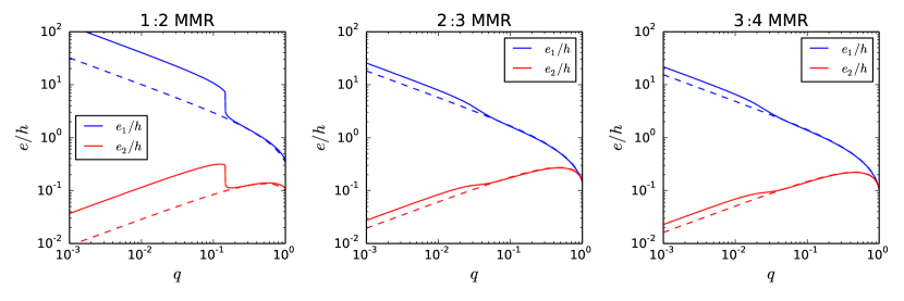
Figure 8: Equilibrium eccentricities vs mass ratio $q=m_{1}/m_{2}$ of the two planets captured into a first-order MMR in a disk with uniform surface density ($\beta=0$ in $\Sigma\propto r^{-\beta}$). Note that the $e_{i}/h$ value depends only on $q$ and is independent of the total mass of the planets and $h$. Only the $q<1$ region is plotted since convergent migration requires $q\lesssim 1$. The blue (red) curve shows the eccentricity of the inner (outer) planet. The solid (dashed) curve shows the eccentricity for the realistic (simple) migration model. These results are calculated under the assumption that eccentricity damping is weak.

Figure 8 shows the equilibrium eccentricities of the two planets calculated using the above method. For the simple migration model, equations (18) and (19) give $e_{1,\rm eq}\sim q^{-1/2}h$ and $e_{2,\rm eq}\sim q^{1/2}h$. At the equilibrium, the $e_{1}^{2}$ terms and the $e_{2}^{2}$ terms in equation (19) are comparable when $q\lesssim 1$: The eccentricity terms in the first line of (19) are comparable to or smaller than the corresponding eccentricity terms in the second line when $q\lesssim 1$, and $qe_{1}^{2}/T_{e,1}\sim e_{2}^{2}/T_{e,1}$ given that $T_{e,1}/T_{e,2}\sim q^{-1}$.

For the realistic migration model, the result is similar to that of the simple migration model when $q$ is relatively large ($q\gtrsim 0.15,0.04$ and $0.03$ for the 1:2, 2:3 and 3:4 MMR respectively). When $q$ is smaller, however, $e_{1,\rm eq}$ exceeds $\sim 3h$ and the damping rate $T_{e,1}^{-1}$ is reduced. Therefore, the equilibrium eccentricities of the planets must increase in order to satisfy equation (19).

The equilibrium always exists when both planets have finite masses, although it may correspond to $e_{1,\rm eq}\gtrsim 1$, which implies that the smaller planet can be ejected due to instability before reaching the equilibrium. This is very different from the “massless inner planet” case considered in Section 3, where the equilibrium state may not exist. The reason of such a difference is that while the eccentricity of the smaller planet can exceed $3h$, the eccentricity of the more massive planet always remains well below $3h$, so that the eccentricity damping from the more massive planet is able to balance migration, ensuring the existence of an equilibrium state.

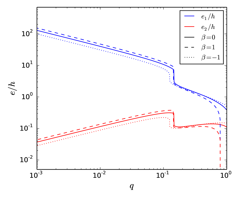
Figure 9: Equilibrium eccentricities of the two planets captured into a 1:2 MMR in disks with different $\beta$. The blue (red) curves show the eccentricities of the inner (outer) planet. The solid, dashed and dotted curves are the eccentricities for $\beta=0,1$ and $-1$ respectively. The results are similar for different values of $\beta$.

The equilibrium eccentricities also depend on the density profile of the disk, which is characterized by the parameter $\beta$ [assuming that the disk has $\Sigma(r)\propto r^{-\beta}$; note that we adopt $\beta=0$ everywhere else in this paper]. Figure 9 shows that the equilibrium eccentricities of the planets depend weakly on $\beta$.

4.1.2 Effect of strong eccentricity damping

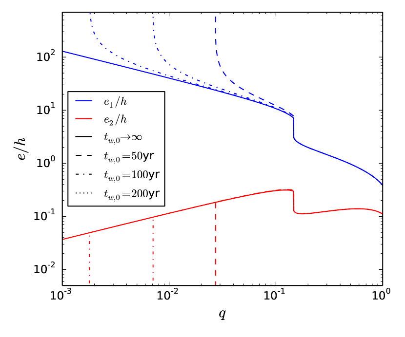
Figure 10: Equilibrium eccentricities of the two planets with $\mu_{1}+\mu_{2}=10^{-3},M_{\star}=1M_{\odot}$ and $a_{2}=1$ au captured into the 1:2 MMR in a disk with uniform surface density, for different strengths of eccentricity damping. The eccentricity damping rate is characterized by $t_{w,0}$, defined as $t_{\rm wave}$ (see Eqs. 3-6) evaluated at $m=m_{1}+m_{2}$ and $a=a_{2}$. The blue (red) curves show the eccentricity of the inner (outer) planet. Different line styles correspond to different $t_{w,0}$, with the solid curves corresponding to very slow migration ($t_{w,0}\to\infty$).

When $q$ is small, the resonant perturbation from the inner planet is no longer much stronger than the eccentricity damping of the outer planet, and the second term in (17) can no longer be ignored. In this regime, the equilibrium eccentricities can be significantly affected when the realistic migration model is applied.

For sufficiently small $q$ (which gives large $e_{1}/h$), the terms proportional to $e_{1}^{2}$ in equation (19) are negligible, so $e_{2,\rm eq}\sim q^{1/2}h$ can be determined directly from (19) and is independent of the strength of eccentricity damping. Meanwhile, equations (17) and (18) suggest that for smaller $\mu_{1}$ (or larger $1/T_{e,2}$), $|\sin\theta_{2}|$ increases, $|\cos\theta_{2}|$ decreases, and $e_{1,\rm eq}/e_{2,\rm eq}$ increases. In particular, when $\mu_{1}$ is sufficiently small (i.e. $\mu_{1}n_{2}\sim e_{2,\rm eq}/T_{e,2}\sim q^{1/2}h/T_{e,2}$), $|\cos\theta_{2}|\to 0$ and $e_{1,\rm eq}/e_{2,\rm eq}$ diverges. Since $e_{2,\rm eq}$ is finite, this means that $e_{1,\rm eq}$ diverges (i.e. ejection or collision of the smaller planet should happen before the equilibrium is reached.)

Figure 10 (based on numerical calculations of the equilibrium eccentricities) demonstrates this effect. For given $\mu_{1}+\mu_{2}$ and $n_{1},n_{2}$, the critical $q$ at which $e_{1,\rm eq}$ diverges is related to the characteristic eccentricity damping rate by $q_{\rm crit}\propto t_{w,0}^{-2}$, where $t_{w,0}$ is a timescale characterizing the migration and eccentricity damping defined as $t_{\rm wave}$ [see Eq. (6)] evaluated at $m=m_{1}+m_{2}$ and $a=a_{2}$. Note that $t_{w,0}$ is determined by the disk parameters, and is comparable to $T_{e,0}$ of the larger planet. This scaling for $q_{\rm crit}$ can be explained as follows: The eccentricity of the smaller planet $e_{1,\rm eq}$ diverges when $\cos\theta_{2}\to 0$ according to (18). When $\cos\theta_{2}\to 0$ (and $\sin\theta_{2}\to 1$), equation (17), together with the fact that $e_{2,\rm eq}\sim q^{1/2}h$, gives (assuming $q$ is small)

$$\begin{split}\mu_{1}n_{2}\sim e_{2,\rm eq}/T_{e,2}~{}~{}\Rightarrow~{}~{}q(\mu_{1}+\mu_{2})n_{2}\sim q^{1/2}h/t_{w,0},\end{split}$$ (20)

which then gives $q_{\rm crit}\propto t_{w,0}^{-2}$.

A major caveat of the above calcuation is that the Hamiltonian (12) and the equations for the equilibrium, (16)-(19), only include the lowest-order terms in eccentricities; i.e., we have effectively assumed $e_{1},e_{2}\ll 1$. For realistic systems, when $e_{1}$ becomes large, higher-order secular couplings may affect the result. We will discuss this issue in the next subsection.

4.2 Three-body simulations: effects of nonlinear eccentricities and non-adiabatic evolution

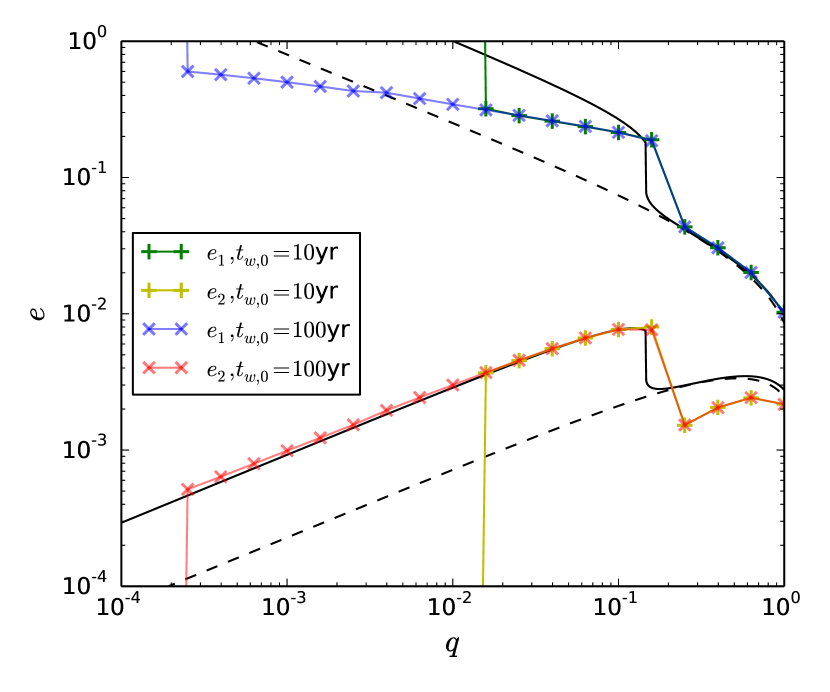
Figure 11: Equilibrium eccentricities of two planets with $\mu_{1}+\mu_{2}=10^{-3},M_{\star}=1M_{\odot}$ and initial $a_{2}=1$ au captured into the 1:2 MMR in a disk with uniform surface density and $h=0.025$. The black curves show our analytical results, as given in Fig. 8. The 3-body integration results for $t_{w,0}=10$ yr (100yr) are shown in crosses (saltires). For $t_{w,0}=10$ yr, $e_{1}$ ($e_{2}$) is marked by the blue (red) curve; for $t_{w,0}=100$ yr, $e_{1}$ ($e_{2}$) is marked by the green (yellow) curve. When the inner planet is ejected (or collides with the other planet or the star), we set $e_{1}=\infty$ and $e_{2}=0$.

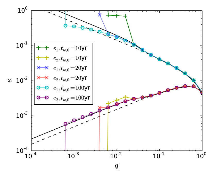
Figure 12: Same as Fig. 11, but for the 2:3 MMR. The behavior of the system is slightly different; see the text for more discussion.

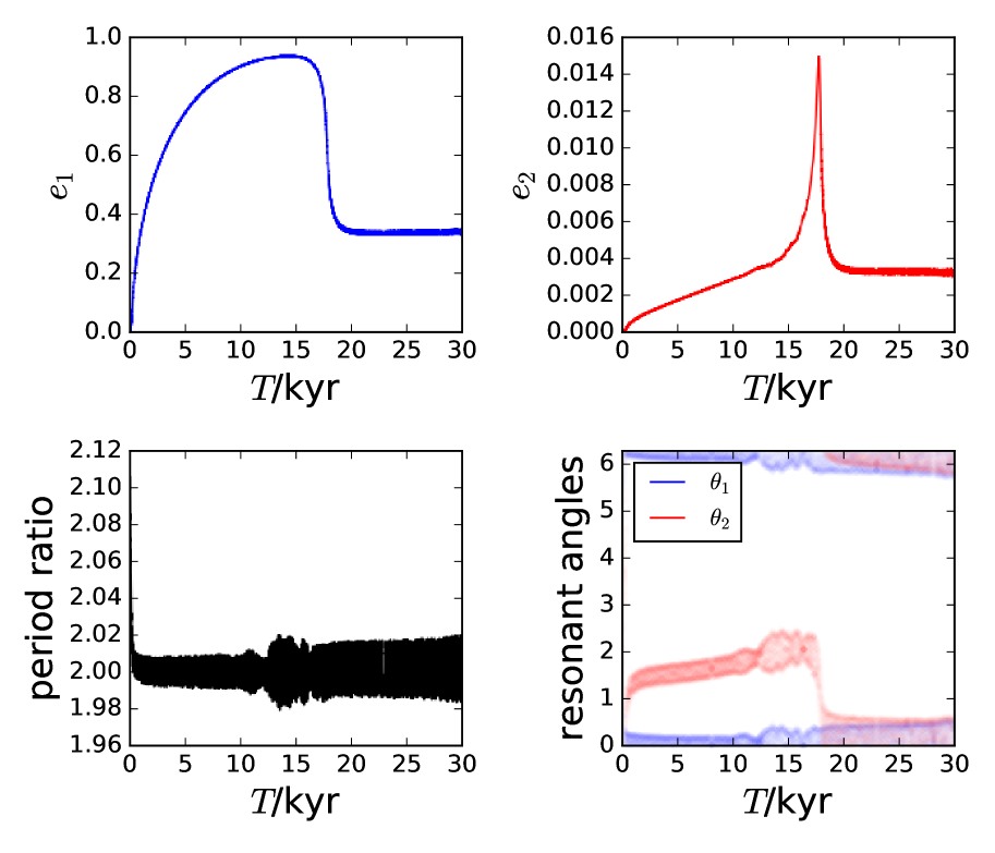
Figure 13: An example where the eccentricity $e_{1}$ overshoots to a large value before reaching equilibrium, for the system in Fig. 11 with $t_{w,0}=10$ yr and $q=0.125$. The different panels show the two planet’s eccentricities ($e_{1},e_{2}$), the period ratio and the resonant angles ($\theta_{1}=2\lambda_{2}-\lambda_{1}-\varpi_{1}$, $\theta_{2}=2\lambda_{2}-\lambda_{1}-\varpi_{2}$). In this example, $e_{1}$ reaches a maximum value of $0.935$ before decreasing to the equilibrium value. Note that for a slightly smaller $q$, the inner planet will have $e_{1}\to 1$ and become unstable during the overshoot.

We now use 3-body simulations to check our semi-analytical results obtained in the previous subsection. This is necessary since the Hamiltonian (12) assumes that the eccentricities are small, which may lead to nontrivial errors when $e_{1}$ attains large values. In addition, it is useful to use 3-body integrations to investigate at which point and for what reason(s) the inner planet becomes dynamically unstable at high eccentricities.

Figures 11 and 12 compare the 3-body integration results for the 1:2 and 2:3 MMRs using MERCURY with our analytical results. Forcing due to planet-disk interaction is implemented as described in Cresswell & Nelson (2008) to agree with equations (3) and (4). Overall, the 3-body integration results agree with our analytical results, showing the general trend that the equilibrium eccentricities increase (compared to the simple migration model) for small $q$. However, there are several important effects that the semi-anaytical linear theory fails to capture, and we discuss these effects below.

4.2.1 Effect of high-order coupling at large $e_{1}$

Figure 11 and the $t_{w,0}=100$yr curves in Figure 12 show that $e_{1,\rm eq}$ is smaller than the analytical prediction when $e_{1,\rm eq}\sim 1$. This is likely due to the higher-order secular coupling between the planets; such coupling prevents $e_{1}$ from reaching unity while $e_{2}$ remains finite. As a result, the divergence of $e_{1}$ due to finite eccentricity damping (discussed in Section 4.1.2) does not occur in real systems. (The ejection of the inner planet for small $q$ depicted in Figure 11 and Figure 12 are due to eccentricity overshoot, a phenomenon we will discuss next.)

4.2.2 Effect of non-adiabatic evolution: eccentricity overshoot

For sufficiently slow migration, the evolution of the system is adiabatic (i.e. the evolution of $\eta$, the “resonance depth” parameter, is sufficiently slow so that the system stays close to the libration center as the libration center moves in the phase space) and the eccentricities of both planets should slowly increase until they reach the equilibrium values. In this case, the equilibrium eccentricities are the maximum eccentricities that the planets can reach. However, when $q$ is small or when migration is fast (i.e. $t_{w,0}$ is small), the growth of $e_{2}$ is too slow, and the initial evolution of $e_{1}$ is similar to the restricted problem studied in Section 3: Due to the inefficient eccentricity damping, $\eta$ and $e_{1}$ both keep increasing, and $e_{1}$ can easily grow beyond the equilibrium value. The growth of $e_{1}$ stops only when it becomes so large that the secular interaction between the planets forces $e_{2}$ to increase. Since eccentricity damping of $e_{2}$ is still efficient, this stops the system from going deeper into the resonance (i.e. stops $\eta$ from further increasing). Eventually, the system will reach equilibrium, provided that the smaller planet has not become dynamically unstable during the high-$e_{1}$ phase.

Figure 13 shows an example. Before the system reaches equilibrium, the eccentricity $e_{1}$ first overshoots to a very large value, then decreases back to the equilibrium value. When $q$ is smaller (or when the migration is faster), the inner planet will be ejected because it reaches $e_{1}\to 1$ during this overshooting phase. This is the reason for the ejection of the smaller planet at low $q$ in Figures 11 and 12.

It is worth noting that significant eccentricity overshoot is a phenomenon unique to the realistic migration model. For the simple migration model, since the eccentricity damping of the inner planet is efficient (i.e. $e_{1}^{2}/T_{e,1}$ always increases as $e_{1}$ increases), the system will cease to go deeper into the resonance once the $e_{1}^{2}$ terms in equation (19) can balance the migration; this corresponds to an insignificant eccentricity overshoot.

4.2.3 Effect of non-adiabatic evolution: bifurcation of the equilibrium state

In Figure 12, we observe that the equilibrium eccentricity of the small planet increases abruptly when $q$ goes below $q\simeq 0.02$ (0.005) for $t_{w,0}=10$ yr (20 yr); at a somewhat smaller $q$ the system becomes unstable. It is likely that this abrupt change corresponds to a bifurcation, with the equilibrium states before and after the bifurcation corresponding to two different fixed points of the system. One possible reason for this bifurcation is that the finite migration rate, together with the more realistic migration model, affect the stability of the fixed points. This different equilibrium state with a higher equilibrium eccentricity is not captured by our analytical result. Also, for this new equilibrium state we observe less eccentricity overshoot.

As $t_{w,0}$ increases, the intermediate region where the system reaches this different equilibrium state with high eccentricity shrinks; when $t_{w,0}$ is sufficiently large the system always becomes unstable (due to eccentricity overshoot) before the bifurcation happens and this intermediate region disappears.

4.3 Stability of capture

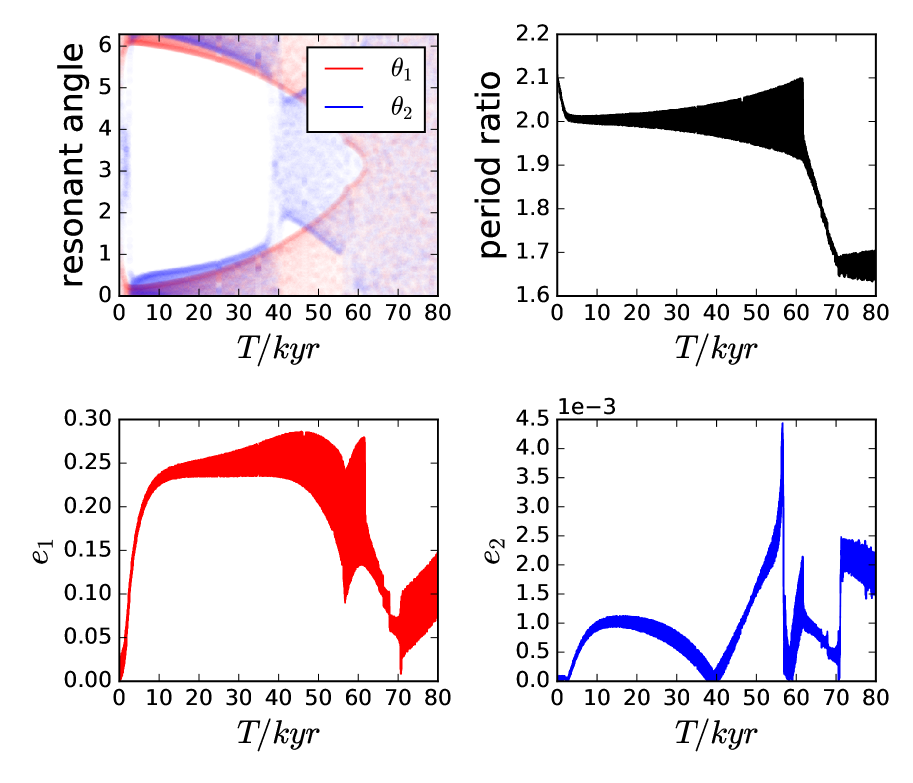
Figure 14: Outcome of the 1:2 MMR capture for the system depicted in Fig. 11 with $q=0.01$ and $t_{w,0}=100$ yr, using the simple migration model. We see that the system escapes the resonance at $t\simeq 60$ kyr.

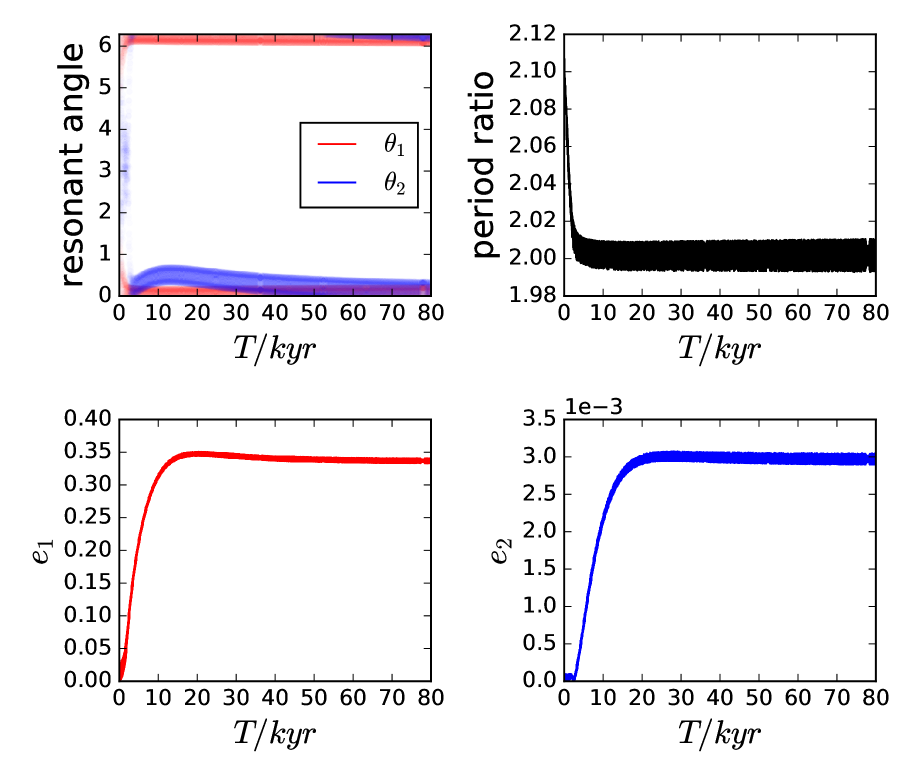
Figure 15: Same as Fig. 14, except that the realistic migration model is used. The equilibrium state is stable. Note that the equilibrium eccentricity also is increased compared to Figure 14.

Similar to the case when the smaller planet is massless (Section 3), using the realistic migration model affects the stability of MMR capture. We observe that when the equilibrium eccentricity is $\gtrsim$ a few $h$, the system tends to be more stable compared to the prediction of the simple migration model. Since it is difficult to do a thorough survey of the parameter space, we illustrate this by an example. Figures 14 and 15 show the different outcomes of a 1:2 MMR capture when the simple migration model (eccentricity-independent $T_{e}$ and $T_{m}$) and the realistic migration model (eccentricity-dependent $T_{e}$ and $T_{m}$) are used. For the simple migration model, the equilibrium state is overstable, and the system eventually escapes the resonance. For the realistic migration model, the equilibrium state becomes stable (the eccentricity at the equilibrium also increases compared to the simple migration model).

Moreover, all numerical examples summarized in Figs. 11 and 12 (except those caese where the inner planet is ejected) have stable equilibrium states. This suggests that for planets undergoing type-I migration, the capture into a first-order MMR is stable for typical disk configurations if we use the realistic migration model. By contrast, if we use the simple migration model for the systems in Figs. 11 and 12, the equilibrium state becomes unstable for $q\lesssim 0.1$.

Deck & Batygin (2015) have previously carried out an extensive study on the stability of the equilibrium state of first-order MMRs for general planet mass ratios. Their analysis was entirely based on the simple migration model. They found a region of the parameter space leading to overstability and proposed a criterion for overstability of the equilibrium state. Since an overstable system tends to evolve to an adjacent MMR equilibrium state, they concluded that the overstability of the equilibrium state cannot fully explain the observed paucity of resonant pairs in the Kepler sample.

However, the overstability criterion of Deck & Batygin (2015) cannot be directly generalized to the realistic migration model (with eccentricity-dependent $T_{m},T_{e}$). This is because the stability of the equilibrium state depends on both $\dot{a}/a,\dot{e}/e$ at the equilibrium and their partial derivatives with respect to the eccentricity. Although it is possible to tune the parameters of the simple migration model ($T_{e,0},~{}T_{m,0}$ for each planet and $p$) to obtain $\dot{a}/a,\dot{e}/e$ and $\partial(\dot{a}/a)/\partial e$ that locally match the values for the realistic migration model near the equilibrium, the local value of $\partial(\dot{e}/e)/\partial e$ in general cannot be matched by tuning the parameters of the simple migration model. Still, if we oversimplify the problem by plugging the local values of $T_{e},~{}T_{m}$ at the equilibrium into the overstability criterion of Deck & Batygin (2015), the stability does tend to increase compared to the simple migration model (with $T_{e}=T_{e,0},~{}T_{m}=T_{m,0}$) when $e_{1}\gtrsim$ a few $h$. This is mainly because $T_{e}$ of the inner planet for the realistic migration model is larger than that for the simple migration model, which pushes the system away from the instability zone (see Figures 2 and 3 of Deck & Batygin 2015). Note that this is only an intuitive explanation of our finding of the increased stability and cannot serve as a rigorous analysis.

5 Summary and discussion

5.1 Summary of key results

In this paper we have carried out theoretical and numerical studies on the outcomes of first-order MMR capture for planets undergoing convergent type-I migration. Unlike previous works (Goldreich & Schlichting, 2014; Deck & Batygin, 2015; Delisle et al., 2015; Xu & Lai, 2017) which adopted a simple migration model where the eccentricity damping rate and orbit decay rate [$T_{e}^{-1}$ and $T_{m}^{-1}$ respectively, see equations (1) and (2)] are independent of the planet’s eccentricity, we consider a more realistic model for $T_{e}$ and $T_{m}$ which captures their nonlinear eccentricity dependence when the eccentricity exceeds $\sim h$ (where $h\equiv H/r$ is the aspect ratio of the disk). We find that this more realistic migration model can significantly affect the outcomes of MMR capture and lead to several new dynamical behaviors.

First, the equilibrium eccentricities of planets captured into the MMR can be larger by a factor of a few than those predicted by the simple migration model (which assumes eccentricity-independent $T_{e},T_{m}$). This arises because when $e\gtrsim 3h$, eccentricity damping becomes weaker and the system migrates deeper into the resonance before reaching equilibrium. When the inner planet is massless, the equilibrium state no longer exists if the equilibrium eccentricity predicted using the simple migration model is $\gtrsim 3h$, and the planet’s eccentricity grows and eventually becomes unstable (Section 3.1). For general planet mass ratios (section 4), the more massive planet’s eccentricity stays below $3h$, and the eccentricity damping of this more massive planet ensures the existence of the equilibrium state. However, the equilibrium eccentricity is larger than the prediction using the simple migration model when the mass ratio $q=m_{1}/m_{2}$ is sufficiently small (Section 4.1). This increase in eccentricity is very significant for the 1:2 MMR, and less significant for other first-order MMRs (see Fig. 8). For typical disk parameters, the critical mass ratio below which such increase occur is around $0.03-0.15$ (see Figs. 8-9).

Second, the stability of the equilibrium state can be strongly affected by the migration model. Our analytical calculation and parameter survey for the case when the inner planet is massless (Section 3) show that the equilibrium state becomes more stable when the equilibrium eccentricity is $e_{\rm eq}\gtrsim 2h$ (Section 3.2; see Fig. 3). This increased level of stability of MMR is also seen when both planets have finite masses (Section 4.3). In particular, for realistic disk configurations, the simple migration model predicts that the equilibrium state is unstable for small $q$, while the realistic migration model predicts that the equilibrium state is virtually always stable (provided that the small planet does not suffer dynamical ejection at high eccentricities; see below).

Another new phenomenon we have found is that when the migration is fast and/or the inner planet’s mass is sufficiently small, the eccentricity growth of the more massive planet (due to the resonant perturbation from the inner, smaller planet) becomes too slow; this causes the eccentricity of the smaller planet to overshoot the equilibrium value before the system reaches the equilibrium state (Section 4.2.2; see Fig. 13). Such an overshoot can be very significant and may cause the smaller planet to be ejected at high eccentricities even when the equilibrium eccentricity is modest.

Overall, using the more realistic migration model tends to increase the equilibrium eccentricities of planets captured in MMRs and make the equilibrium state less prone to overstability. However, when migration is sufficiently fast (or the small planet has too small a mass), it also causes the ejection of the smaller planet during eccentricity overshoot — this behavior is much less significant when the simple migration model is used. All of these can affect the ways in which MMRs shape planetary system architecture.

5.2 Implications for multi-planet system architecture

5.2.1 Occurrence of MMRs

For planets with similar masses ($q\sim 1$), since the equilibrium eccentricities of the planets captured into MMRs are usually small, previous results concerning the stability of MMRs remain valid (Deck & Batygin, 2015; Delisle et al., 2015; Xu & Lai, 2017).

For smaller mass ratio ($q\lesssim 0.1$), however, the maximum eccentricity that the smaller planet can reach is much larger when the realistic migration model (with eccentricity-dependent $T_{e},~{}T_{m}$) is applied (compared to the results obtained with eccentricity-independent $T_{e},~{}T_{m}$) due to the increased equilibrium eccentricity and eccentricity overshoot. The large eccentricity can lead to the ejection of the smaller planet (when its eccentricity approaches unity) or make it scatter with a third planet in the system (if their orbits cross). This tends to reduce the multiplicity of the system when it initially hosts a pair of convergently migrating planets with small mass ratio. This effect also reduces the number of small-mass-ratio planet pairs in MMRs.

5.2.2 Loneliness of Hot Jupiters

The eccentricity overshoot phenomenon (which occurs when the mass ratio is small and the migration is sufficiently fast) provides an efficient way of removing super-Earth companions of fast migrating giant planets. This may help explain the loneliness (the lack of low-mass planet neighbors) of hot Jupiters (Huang et al., 2016) if they are formed through disk-driven migration. In this picture, hot Jupiters arrived at their current locations through fast type-II migration, with the migration timescale much less than the disk lifetime. If they had any inner low-mass companion (a super-Earth), it could be removed when captured into a MMR with the Jupiter during its migration due to the instability caused by eccentricity overshoot. On the other hand, warm Jupiters do commonly have low-mass planet companions (Huang et al. 2016). This may be explained by their slow migration rates: During such slow migration, their low-mass companions do not suffer eccentricity overshoot and therefore are kept in safety upon capture into MMRs. Note that the rate of type-II migration is sensitive to the property of the disk, especially its viscosity (Ward, 1997). Thus, in this scenario, whether a system forms hot Jupiters (without low-mass companions) or warm Jupiters (with low-mass companions) simply reflects the different disk properties and the resulting different migration history of giant planets.

Of course, hot Jupiters may also form by high-eccentricity migration, in which the eccentricity of a giant planet is excited by distant stellar or planetary companions, followed by tidal circularization and orbital decay (e.g. Dawson & Johnson 2018). In this scenario, the loneliness of hot Jupiters can be naturally explained because a giant planet undergoing high-amplitude eccentricity oscillations can easily eject smaller planets interior of its initial orbit. Our discussion here does not aim to prove or disprove any particular formation scenario; we simply argue that one should not rule out the disk-driven (low-eccentricity) migration scenario using solely the loneliness of Hot Jupiters.

References

- André & Papaloizou (2016) André Q., Papaloizou J. C. B., 2016, MNRAS, 461, 4406
- Batalha et al. (2013) Batalha N. M., et al., 2013, The Astrophysical Journal Supplement Series, 204, 24
- Batygin & Morbidelli (2013) Batygin K., Morbidelli A., 2013, AJ, 145, 1
- Chambers (1999) Chambers J. E., 1999, Monthly Notices of the Royal Astronomical Society, 304, 793
- Chatterjee & Ford (2015) Chatterjee S., Ford E. B., 2015, ApJ, 803, 33
- Coughlin et al. (2016) Coughlin J. L., et al., 2016, ApJS, 224, 12
- Cresswell & Nelson (2008) Cresswell P., Nelson R. P., 2008, A&A, 482, 677
- Cresswell et al. (2007) Cresswell P., Dirksen G., Kley W., Nelson R. P., 2007, A&A, 473, 329
- Crida et al. (2008) Crida A., Sándor Z., Kley W., 2008, A&A, 483, 325
- Dawson & Johnson (2018) Dawson R. I., Johnson J. A., 2018, preprint, (arXiv:1801.06117)
- Deck & Batygin (2015) Deck K. M., Batygin K., 2015, ApJ, 810, 119
- Delisle et al. (2014) Delisle J.-B., Laskar J., Correia A. C. M., 2014, A&A, 566, A137
- Delisle et al. (2015) Delisle J.-B., Correia A. C. M., Laskar J., 2015, A&A, 579, A128
- Fabrycky et al. (2014) Fabrycky D. C., et al., 2014, ApJ, 790, 146
- Goldreich & Schlichting (2014) Goldreich P., Schlichting H. E., 2014, AJ, 147, 32
- Goldreich & Tremaine (1980) Goldreich P., Tremaine S., 1980, ApJ, 241, 425
- Hasegawa & Ida (2013) Hasegawa Y., Ida S., 2013, ApJ, 774, 146
- Huang et al. (2016) Huang C., Wu Y., Triaud A. H., 2016, The Astrophysical Journal, 825, 98
- Izidoro et al. (2017) Izidoro A., Ogihara M., Raymond S. N., Morbidelli A., Pierens A., Bitsch B., Cossou C., Hersant F., 2017, MNRAS, 470, 1750
- Kley et al. (2005) Kley W., Lee M. H., Murray N., Peale S. J., 2005, A&A, 437, 727
- Lega et al. (2015) Lega E., Morbidelli A., Bitsch B., Crida A., Szulágyi J., 2015, MNRAS, 452, 1717
- Lithwick & Wu (2012) Lithwick Y., Wu Y., 2012, ApJ, 756, L11
- Luger et al. (2017) Luger R., et al., 2017, Nature Astronomy, 1, 0129
- Michtchenko & Ferraz-Mello (2001) Michtchenko T. A., Ferraz-Mello S., 2001, Icarus, 149, 357
- Migaszewski (2015) Migaszewski C., 2015, MNRAS, 453, 1632
- Mills et al. (2016) Mills S. M., Fabrycky D. C., Migaszewski C., Ford E. B., Petigura E., Isaacson H., 2016, Nature, 533, 509
- Murray & Dermott (1999) Murray C. D., Dermott S. F., 1999, Solar system dynamics. Cambridge university press
- Papaloizou & Szuszkiewicz (2005) Papaloizou J. C. B., Szuszkiewicz E., 2005, MNRAS, 363, 153
- Pu & Wu (2015) Pu B., Wu Y., 2015, ApJ, 807, 44
- Terquem & Papaloizou (2007) Terquem C., Papaloizou J. C. B., 2007, ApJ, 654, 1110
- Ward (1997) Ward W. R., 1997, Icarus, 126, 261
- Xu & Lai (2017) Xu W., Lai D., 2017, MNRAS, 468, 3223
- Zhang et al. (2014) Zhang X., Li H., Li S., Lin D. N. C., 2014, ApJ, 789, L23