GADAM: Genetic-Evolutionary ADAM for Deep Neural Network Optimization

Abstract

Deep neural network learning can be formulated as a non-convex optimization problem. Existing optimization algorithms, e.g., Adam, can learn the models fast, but may get stuck in local optima easily. In this paper, we introduce a novel optimization algorithm, namely Gadam (Genetic-Evolutionary Adam). Gadam learns deep neural network models based on a number of unit models generations by generations: it trains the unit models with Adam, and evolves them to the new generations with genetic algorithm. We will show that Gadam can effectively jump out of the local optima in the learning process to obtain better solutions, and prove that Gadam can also achieve a very fast convergence. Extensive experiments have been done on various benchmark datasets, and the learning results will demonstrate the effectiveness and efficiency of the Gadam algorithm.

1 Introduction

Adam (Adaptive Momentum Estimation) [17], with sound theoretic foundations, has been widely used as the optimization algorithm in many existing machine learning models, especially the deep neural networks with non-convex objective functions. Formally, learning the variables of deep neural network models can be formally represented as the following optimization problem:

$$\min_{\mathbf{w}\in\mathcal{W}}f(\mathbf{X},\mathbf{y};\mathbf{w}),$$ (1)

where $f(\cdot,\cdot;\mathbf{w})$ denotes the loss function parameterized by variable vector $\mathbf{w}\in\mathcal{W}$ and $\mathbf{X}$, $\mathbf{y}$ denote the features and labels of the data instances respectively. Set $\mathcal{W}$ represents the feasible solution space, which can be $\mathbb{R}^{n}$ for simplicity if there exist no other constraints on the variables.

Adam adopts an iterative learning scheme to update the model variables. In iteration $k$, given a training instance $(\mathbf{x}_{i},y_{i})$ from the training set, the updating equation of variable $\mathbf{w}$ can be represented as

$$\mathbf{w}_{k} =\mathbf{w}_{k-1}-\eta_{k}\frac{\sqrt{1-\beta^{k}_{2}}}{1-\beta^{k}_{1}}\frac{\mathbf{m}_{k-1}}{\sqrt{\mathbf{v}_{k-1}}+\epsilon},\mbox{ where}\begin{cases}\mathbf{m}_{k-1}&=\beta_{1}\mathbf{m}_{k-2}+(1-\beta_{1})\nabla f(\mathbf{x}_{i},{y}_{i};\mathbf{w}_{k-1});\\ \mathbf{v}_{k-1}&=\beta_{2}\mathbf{v}_{k-2}+(1-\beta_{2})\nabla f(\mathbf{x}_{i},{y}_{i};\mathbf{w}_{k-1})^{2}.\end{cases}$$ (2)

where $\mathbf{w}_{k}$ represents the variable in the $k_{th}$ iteration and $\nabla f(\mathbf{x}_{i},y_{i};\mathbf{w}_{k-1})$ denotes the computed gradient of the function regarding variable $\mathbf{w}$ based on the input training instance. Term $\eta_{k}$ is the learning rate, which is usually a small constant. Moment vectors $\mathbf{m}_{k_{1}}$ and $\mathbf{v}_{k-1}$ will be adapted in the learning process, and $\beta_{1}$ and $\beta_{2}$ are the corresponding momentum parameters.

Adam together with its many variants [6, 16] have been shown to be effective for optimizing a large group of problems. However, for the non-convex objective functions of deep learning models, Adam cannot guarantee to identify the globally optimal solutions, whose iterative updating process may inevitably get stuck in local optima. The performance of Adam is not very robust, which will be greatly degraded for the objective function with non-smooth shape or learning scenarios polluted by noisy data. Furthermore, the distributed computation process of Adam requires heavy synchronization, which may hinder its adoption in large-cluster based distributed computational platforms.

On the other hand, genetic algorithm (GA), a metaheuristic algorithm inspired by the process of natural selection in evolutionary algorithms, has also been widely used for learning the solutions of many optimization problems. In GA, a population of candidate solutions will be initialized and evolved towards better ones. Several attempts have also been made to use GA for training deep neural network models [33, 26, 3] instead of the gradient descent based methods. GA has demonstrated its outstanding performance in many learning scenarios, like non-convex objective function containing multiple local optima, objective function with non-smooth shape, as well as a large number of parameters and noisy environments. GA also fits the parallel/distributed computing setting very well, whose learning process can be easily deployed on parallel/distributed computing platforms. Meanwhile, compared with Adam, GA may take more rounds to converge in addressing optimization objective functions.

In this paper, we propose a new optimization algorithm, namely Gadam (Genetic Adaptive Momentum Estimation), which incorporates Adam and GA into a unified learning scheme. Instead of learning one single model solution, Gadam works with a group of potential unit model solutions. In the learning process, Gadam learns the unit models with Adam and evolves them to the new generations with genetic algorithm. In addition, Algorithm Gadam can work in both standalone and parallel/distributed modes, which will also be studied in this paper.

The following part of the paper is organized as follows. In Section 2, we will introduce the related research works about Adam and GA. The detailed learning algorithm Gadam will be introduced in Section 3, whose performance analysis is available in Section 4. In Section 5, we will provide the numerical experiments of Gadam compared with the existing learning algorithms in training several representative deep neural network models. Finally, we will conclude this paper in Section 6.

2 Related Works

Optimization Algorithms: In addressing the optimization problems, SGD (Stochastic Gradient Descent) [23] with sound theoretic foundations has been one of the most frequently used algorithms. Given an objective function $\min_{\mathbf{w}\in\mathcal{W}}f(\mathbf{w})$, SGD adopts an iterative updating schema to learn the model variables as follows:

$$\mathbf{w}_{k}=\mathbf{w}_{k-1}-\eta_{k-1}\cdot\nabla f(\mathbf{w}_{k-1}).$$ (3)

Here, the parameter $\eta_{k}$ is usually a small constant, which is referred to as the learning rate. Meanwhile, to further accelerate the learning process, a variant of SGD, namely SGDM (SGD with Momentum) [27], has been proposed, which updates the variables according to the following equations

$$\mathbf{w}_{k}=\mathbf{w}_{k-1}-\eta_{k}\cdot\mathbf{v}_{k}\mbox{, where }\mathbf{v}_{k}=\beta\cdot\mathbf{v}_{k-1}+\nabla f(\mathbf{w}_{k-1}).$$ (4)

In the equation, $\beta\in[0,1)$ is a momentum parameter and vector $\mathbf{v}_{0}$ is initialized with value $\mathbf{0}$.

SGD and SGDM scale the gradient uniformly in all directions (i.e., all the variables), which makes the tuning of learning rate $\eta_{k}$ very tedious and laborious. To resolve such a problem, several adaptive optimization methods have been proposed, including Adam [17], RMSprop [29] and Adagrad [7], which uses distinct learning rates for different variables. Formally, the variable updating equations adopted in Adagrad [7] and RMSprop [29] can be represented as follows respectively:

$$\begin{cases}&\mbox{\# Adagrad}\\ &\mathbf{w}_{k}=\mathbf{w}_{k-1}-\eta_{k}\cdot\frac{\nabla f(\mathbf{w}_{k-1})}{\sqrt{\mathbf{v}_{k-1}}+\epsilon},\\ &\mathbf{v}_{k-1}=\sum_{j=1}^{k-1}\nabla f(\mathbf{w}_{j})^{2}.\end{cases}\mbox{ }\begin{cases}&\mbox{\# RMSprop}\\ &\mathbf{w}_{k}=\mathbf{w}_{k-1}-\eta_{k}\cdot\frac{\nabla f(\mathbf{w}_{k-1})}{\sqrt{\mathbf{v}_{k-1}}+\epsilon},\\ &\mathbf{v}_{k-1}=\beta\cdot\mathbf{v}_{k-2}+(1-\beta)\cdot\nabla f(\mathbf{w}_{k-1})^{2}.\end{cases}$$ (5)

In Adagrad, vector $\mathbf{v}_{k}$ increases monotonically as the update iteration continues, and its scaling factor will keep decreasing when updating vector $\mathbf{w}_{k}$. RMSprop addresses the problem by employing an average scale instead of a cumulative scale, and Adam [17] resolves such a problem with a bias correction, which adopts an exponential moving average for the step in lieu of the gradient.

Genetic Algorithms: In the 50s in the last century, computer scientists proposed that evolutionary systems with the idea that evolution could be used as an optimization tool for engineering problems. The central idea in all these systems was to evolve a population of candidate solutions to a given problem with the operations inspired by the natural genetic variation and selection. Genetic algorithm [14] invented by John Holland is one of the most important algorithms proposed in the evolutionary computing. A detailed introduction to classic genetic algorithm is available in [21]. In recent years, some research works proposed to apply genetic to evolve neural network models. Eli et al. propose to extend previous work and propose a genetic algorithm assisted method for deep learning [2, 26]. In [33], Zhang et al. introduce a evolutionary network model as an alternative approach to deep learning models based on data sampling, genetic model learning and ensemble learning.

Deep Learning: The essence of deep learning is to compute hierarchical features or representations of the observational data [9, 19]. With the surge of deep learning research and applications in recent years, lots of research works have appeared to apply the deep learning methods, like deep belief network [12], deep Boltzmann machine [24], deep neural network [15, 18] and deep autoencoder model [30], in various applications. The representative deep neural network models studied nowadays include the convolutional neural network (CNN) [20, 18], recurrent neural network (RNN), long-short term memory (LSTM) [13], deep feedforward neural network [8], and deep auto-encoder model [30]. These deep neural network models have achieved remarkable performance in various application domains, like speech and audio processing [5, 11], language processing [1, 22], information retrieval [10, 24], computer vision [19], as well as multimodal and multi-task learning [31, 32].

3 Proposed Methods

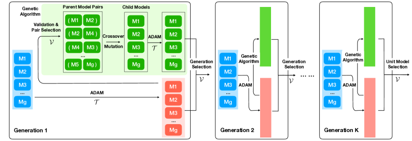
Figure 1: Overall Architecture of Gadam Model.

The overall framework of the model learning process in Gadam is illustrated in Figure 1, which involves multiple learning generations. In each generation, a group of unit model variable will be learned with Adam from the data, which will also get evolved effectively via the genetic algorithm. Good candidate variables will be selected to form the next generation. Such an iterative model learning process continues until convergence, and the optimal unit model variable at the final generation will be selected as the output model solution. For simplicity, in this paper, we will refer to unit models and their variables interchangeably without distinguishing their differences.

3.1 Model Population Initialization

Gadam learns the optimal model variables based on a set of unit models (i.e., variables of these unit models by default), namely the unit model population, where the initial unit model generation can be denoted as set $\mathcal{G}^{(0)}=\{M^{(0)}_{1},M^{(0)}_{2},\cdots,M^{(0)}_{g}\}$ ($g$ is the population size and the superscript represents the generation index). Based on the initial generation, Gadam will evolve the unit models to new generations, which can be represented as $\mathcal{G}^{(1)},\mathcal{G}^{(2)},\cdots,\mathcal{G}^{(K)}$ respectively. Here, parameter $K$ denotes the total generation number.

For each unit model in the initial generation $\mathcal{G}^{(0)}$, e.g., $M^{(0)}_{i}$, we can initialize its variables $\mathbf{w}^{(0)}_{i}$ with random values sampled from certain distributions (e.g., the standard normal distribution). These initial generation serve as the starting search points, from which Gadam will expand to other regions to identify the optimal solutions. Meanwhile, for the unit models in the following generations, their variable values will be generated via GA from their parent models respectively.

3.2 Model Learning with Adam

In the learning process, given any model generation $\mathcal{G}^{(k)}$ ($k\in\{1,2,\cdots,K\}$), Gadam will learn the (locally) optimal variables for each unit model with Adam. Formally, Gadam trains the unit models with several epochs. In each epoch, for each unit model $M^{(k)}_{i}\in\mathcal{G}^{(k)}$, a separated training batch will be randomly sampled from the training dataset, which can be denoted as $\mathcal{B}=\{(\mathbf{x}_{1},\mathbf{y}_{1}),(\mathbf{x}_{2},\mathbf{y}_{2}),\cdots,(\mathbf{x}_{b},\mathbf{y}_{b})\}\subset\mathcal{T}$ (here, $b$ denotes the batch size and $\mathcal{T}$ represents the complete training set). Let the loss function introduced by unit model $M^{(k)}_{i}$ for instance $(\mathbf{x}_{j},\mathbf{y}_{j})$ be $f(\mathbf{x}_{j},\mathbf{y}_{j};\mathbf{w}_{i}^{(k)})$, and we can represent the learned model variable vector by the training instance as

$$\bar{\mathbf{w}}_{i}^{(k)}=Adam\left(f(\mathbf{x}_{j},\mathbf{y}_{j};\mathbf{w}_{i}^{(k)});\mathcal{B}\right).$$ (6)

Depending on the specific unit models and application settings, the loss function will have different representations, e.g., mean square loss, hinge loss or cross entropy loss. In this paper, we will illustrate Gadam as a general learning algorithm without providing the concrete loss representations. Such a learning process continues until convergence, and we can represent the updated model generation $\mathcal{G}^{(k)}$ with (locally) optimal variables as $\bar{\mathcal{G}}^{(k)}=\{\bar{M}^{(k)}_{1},\bar{M}^{(k)}_{2},\cdots,\bar{M}^{(k)}_{g}\}$, whose corresponding variable vectors can be denoted as $\{\bar{\mathbf{w}}^{(k)}_{1},\bar{\mathbf{w}}^{(k)}_{2},\cdots,\bar{\mathbf{w}}^{(k)}_{g}\}$ respectively.

3.3 Model Evolution with Genetic Algorithm

In this part, based on the learned unit models, i.e., $\bar{\mathcal{G}}^{(k)}$, we propose to further search for better solutions for the unit models effectively via the genetic algorithm.

3.3.1 Model Fitness Evaluation

Unit models with good performance may fit the learning task better. Instead of evolving models randomly, Gadam proposes to pick good unit models from the current generation to evolve. Based on a sampled validation batch $\mathcal{V}\subset\mathcal{T}$, the fitness score of unit models, e.g., $\bar{M}^{(k)}_{i}$, can be effectively computed based on its loss terms introduced on $\mathcal{V}$ as follows

$$\mathcal{L}^{(k)}_{i}=\mathcal{L}(\bar{M}^{(k)}_{i};\mathcal{V})=\sum_{(\mathbf{x}_{j},\mathbf{y}_{j})\in\mathcal{V}}l(\mathbf{x}_{j},\mathbf{y}_{j};\bar{\mathbf{w}}_{i}^{(k)}).$$ (7)

Based on the computed loss values, the selection probability of unit model $\bar{M}^{(k)}_{i}$ can be defined with the following softmax equation

$$P(\bar{M}^{(k)}_{i})=\frac{\exp^{(-\hat{\mathcal{L}}^{(k)}_{i})}}{\sum_{j=1}^{g}\exp^{(-\hat{\mathcal{L}}^{(k)}_{j})}}.$$ (8)

Necessary normalization of the loss values is usually required in real-world applications, as $\exp^{(-{\mathcal{L}}^{(k)}_{i})}$ may approach $0$ or $\infty$ for extremely large positive or small negative loss values ${\mathcal{L}}^{(k)}_{i}$. As indicated in the probability equation, the normalized loss terms of all unit models can be formally represented as $[\hat{\mathcal{L}}^{(k)}_{1},\hat{\mathcal{L}}^{(k)}_{2},\cdots,\hat{\mathcal{L}}^{(k)}_{g}]^{\top}$, where $\hat{\mathcal{L}}^{(k)}_{i}\in[0,1],\forall i\in\{1,2,\cdots,g\}$. According to the computed probabilities, from the unit model set $\bar{\mathcal{G}}^{(k)}$, $g$ pairs of unit models will be selected with replacement as the parent models for evolution, which can be denoted as $\mathcal{P}=\{(\bar{M}^{(k)}_{i_{1}},\bar{M}^{(k)}_{j_{1}}),(\bar{M}^{(k)}_{i_{2}},\bar{M}^{(k)}_{j_{2}}),\cdots,(\bar{M}^{(k)}_{i_{g}},\bar{M}^{(k)}_{j_{g}})\}$.

3.3.2 Unit Model Crossover

Given a unit model pair, e.g., $(\bar{M}^{(k)}_{i_{p}},\bar{M}^{(k)}_{j_{p}})\in\mathcal{P}$, Gadam inherits their variables to the child model via the crossover operation. In crossover, the parent models, i.e., $\bar{M}^{(k)}_{i_{p}}$ and $\bar{M}^{(k)}_{j_{p}}$, will also compete with each other, where the parent model with better performance tend to have more advantages. We can represent the child model generated from $(\bar{M}^{(k)}_{i_{p}},\bar{M}^{(k)}_{j_{p}})$ as $\tilde{M}^{(k)}_{p}$. For each entry in the weight variable $\tilde{\mathbf{w}}^{(k)}_{p}$ of the child model $\tilde{M}^{(k)}_{p}$, Gadam initializes its values as follows:

$$\tilde{w}^{(k)}_{p}[m]=\mathbbm{1}(\mbox{rand}\leq p_{i_{p},j_{p}}^{(k)})\cdot\bar{w}^{(k)}_{i_{p}}[m]+\mathbbm{1}(\mbox{rand}>p_{i_{p},j_{p}}^{(k)})\cdot\bar{w}^{(k)}_{j_{p}}[m].$$ (9)

In the equation, binary function $\mathbbm{1}(\cdot)$ returns $1$ iff the condition holds. Term “rand” denotes a random number in $[0,1]$. The probability threshold $p_{i_{p},j_{p}}^{(k)}$ is defined based on the parent models’ performance:

$$p_{i_{p},j_{p}}^{(k)}=\frac{\exp^{(-\hat{\mathcal{L}}^{(k)}_{i_{p}})}}{\exp^{(-\hat{\mathcal{L}}^{(k)}_{i_{p}})}+\exp^{(-\hat{\mathcal{L}}^{(k)}_{j_{p}})}}.$$ (10)

If $\hat{\mathcal{L}}^{(k)}_{i_{p}}>\hat{\mathcal{L}}^{(k)}_{j_{p}}$, i.e., model $\bar{M}_{i_{p}}^{(k)}$ introduces a larger loss than $\bar{M}_{j_{p}}^{(k)}$, we will have $0<p_{i_{p},j_{p}}^{(k)}<\frac{1}{2}$.

With such a process, based on the whole parent model pairs in set $\mathcal{P}$, we will be able to generate the children model set as set $\tilde{\mathcal{G}}^{(k)}=\{\tilde{M}^{(k)}_{1},\tilde{M}^{(k)}_{2},\cdots,\tilde{M}^{(k)}_{g}\}$.

3.3.3 Unit Model Mutation

To avoid the unit models getting stuck in local optimal points, Gadam adopts an operation called mutation to adjust variable values of the generated children models in set $\{\tilde{M}^{(k)}_{1},\tilde{M}^{(k)}_{2},\cdots,\tilde{M}^{(k)}_{g}\}$. Formally, for each child model $\tilde{M}^{(k)}_{q}$ parameterized with vector $\tilde{\mathbf{w}}^{(k)}_{q}$, we propose to mutate the variable vector according to the following equation, where its $m_{th}$ entry can be updated as

$$\tilde{{w}}^{(k)}_{q}[m]=\mathbbm{1}(\mbox{rand}\leq p_{q})\cdot\mbox{rand}(0,1)+\mathbbm{1}(\mbox{rand}>p)\cdot\tilde{{w}}^{(k)}_{q}[m],$$ (11)

In the equation, term $p_{q}$ denotes the mutation rate, which is strongly correlated with the parent models’ performance:

$$p_{q}=p\cdot\left(1-P(\bar{M}^{(k)}_{i_{q}})-P(\bar{M}^{(k)}_{j_{q}})\right).$$ (12)

For the child models with good parent models, they will have lower mutation rates. Term $p$ denotes the base mutation rate which is usually a small value, e.g., $0.01$, and probabilities $P(\bar{M}^{(k)}_{i_{q}})$ and $P(\bar{M}^{(k)}_{j_{q}})$ are defined in Equ 8. These unit models will be further trained with Adam until convergence, which will lead to the $k_{th}$ children model generation $\tilde{\mathcal{G}}^{(k)}=\{\tilde{M}^{(k)}_{1},\tilde{M}^{(k)}_{2},\cdots,\tilde{M}^{(k)}_{g}\}$.

3.4 New Generation Selection and Evolution Stop Criteria

Among these learned unit models in sets $\bar{\mathcal{G}}^{(k)}=\{\bar{M}^{(k)}_{1},\bar{M}^{(k)}_{2},\cdots,\bar{M}^{(k)}_{g}\}$ and $\tilde{\mathcal{G}}^{(k)}=\{\tilde{M}^{(k)}_{1},\tilde{M}^{(k)}_{2},\cdots,\tilde{M}^{(k)}_{g}\}$, we will re-evaluate their fitness scores based on a shared new validation batch. Among all the unit models in $\bar{\mathcal{G}}^{(k)}\cup\tilde{\mathcal{G}}^{(k)}$, the top $g$ unit models will be selected to form the $(k+1)_{th}$ generation, which can be formally represented as set $\mathcal{G}^{(k+1)}=\{M^{(k+1)}_{1},M^{(k+1)}_{2},\cdots,M^{(k+1)}_{g}\}$. Such an evolutionary learning process will stop if the maximum generation number has reached or there is no significant improvement between consequential generations, e.g., $\mathcal{G}^{(k)}$ and $\mathcal{G}^{(k+1)}$:

$$\Bigg{|}\sum_{M^{(k)}_{i}\in\mathcal{G}^{(k)}}\mathcal{L}^{(k)}_{i}-\sum_{M^{(k+1)}_{i}\in\mathcal{G}^{(k+1)}}\mathcal{L}^{(k+1)}_{i}\Bigg{|}\leq\theta,$$ (13)

The above equation defines the stop criterion of Gadam, where $\theta$ is the evolution stop threshold.

4 Optimization Algorithm Analysis

Figure 2: Analysis of Gadam Algorithm.

In this section, we will analyze the optimization algorithm Gadam from the performance, convergence and parallel/distributed deployment perspectives respectively.

4.1 Learning Algorithm Performance Analysis

The optimization algorithm Gadam proposed in this paper actually incorporate the advantages of both Adam and genetic algorithm. With Adam, the unit models can effectively achieve the (locally/globally) optimal solutions very fast with a few training epochs. Meanwhile, via genetic algorithm based on a number of unit models, it will also provide the opportunity to search for solutions from multiple starting points and jump out from the local optima.

In Figure 2, we compare Gadam with Adam to illustrate its advantages. First of all, as shown in the left 2 plots in Figure 2, different from the traditional Adam algorithm with one single starting point, Gadam involves multiple starting points (i.e., multiple unit models) to search for the optima simultaneously. Both Adam and Gadam are based on the adaptive gradient descent to update the variables by following the function gradient. With more starting points, Gadam will have a larger chance to achieve the globally optimal solution, i.e., the green dot.

In the right two plots, we use a 2-variable function to illustrate that Gadam may jump out from the local optima via crossover and mutation. As shown in the plots, the loss function $f(\cdot,[w_{1},w_{2}])$ is non-convex and has multiple local minima and one global minimum (i.e., the green dot). In the $3_{rd}$ plot, given two starting points (i.e., the grey dots), by following the gradient direction, Gadam will be able to update its variables and move to the local minima (i.e., dots $A$ and $B$). Via crossover, a child model can be generated from the parent models, which is denoted by the blue dot in the plot. For the new child unit model, it inherits $w_{1}$ value from $A$ and $w_{2}$ value from $B$, which lies in a new region. By following the gradient from the new point, the global optimal point will be reached. Meanwhile, in the right plot, given a generated child model parameterized by the blue dot, via the mutation operation, it will be able to jump out from the local minimal region to point $C$, from which the global optimum will be achieved.

Optimization Algorithms	Avg. Loss	Accuracy Rate%
Gadam	0.0396	99.37
Adam	0.0662	99.18
SGD	0.2166	94.51
RMSProp	0.0745	99.00
AdaGrad	0.1720	95.96
AdaDelta	1.8888	66.08
Existing Methods	Avg. Loss	Accuracy Rate%
LeNet-5 (GD)	N.A.	99.05 [20]
gcForest	N.A.	99.26 [34]
Deep Belief Net	N.A.	98.75 [12]
Random Forest	N.A.	96.8 [34]
SVM (rbf)	N.A.	98.60 [4]

Table 1: Performance of Comparison Optimization Algorithms on the Testing Set.

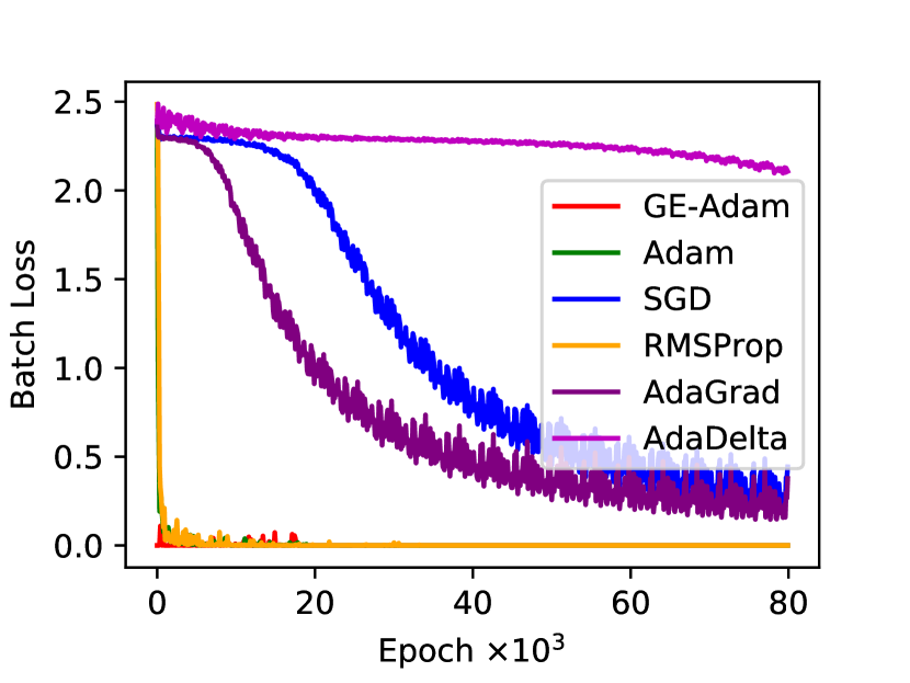
Table 2: Training Loss of Comparison Optimization Algorithms.

4.2 Convergence Analysis

According to [17], for a smooth function, Adam will converge as the function gradient vanishes. On the other hand, the genetic algorithm can also converge according to [28]. Based on these prior knowledge, we can prove the convergence of Gadam as follows.

Theorem 1

Model Gadam will converge in a finite number of evolution rounds.

Proof 1

To prove the above theorem, we only need to prove that the loss term $\mathcal{L}^{(k)}$ for generation $\mathcal{G}^{(k)}$ in Gadam will keep decreasing. Given the $k_{th}$ model generations $\mathcal{G}^{(k)}$, we can denote their introduced loss terms before and after model learning (with Adam) as follows:

$$\mathcal{L}^{(k)}=\sum_{M^{(k)}_{i}\in\mathcal{G}^{(k)}}\mathcal{L}^{(k)}_{i}\mbox{, and }\bar{\mathcal{L}}^{(k)}=\sum_{\bar{M}^{(k)}_{i}\in\bar{\mathcal{G}}^{(k)}}\mathcal{L}^{(k)}_{i}.$$ (14)

According to [17], the variables learned by Adam will converge in variable learning, and we have loss term $\bar{\mathcal{L}}^{(k)}$ after learning will be relatively lower than $\mathcal{L}^{(k)}$, i.e., $\bar{\mathcal{L}}^{(k)}\leq{\mathcal{L}}^{(k)}$.

Meanwhile, in the model evolution, we know that generation $\mathcal{G}^{(k+1)}$ involves the top $g$ unit models selected from its previous generation $\bar{\mathcal{G}}^{(k+1)}\cup\tilde{\mathcal{G}}^{(k+1)}$. Therefore, we have

$$\mathcal{L}^{(k+1)}\leq\bar{\mathcal{L}}^{(k)}\mbox{, where }\mathcal{L}^{(k+1)}=\sum_{M^{(k+1)}_{i}\in\mathcal{G}^{(k+1)}}\mathcal{L}^{(k+1)}_{i}.$$ (15)

In other words, we know $\mathcal{L}^{(k+1)}\leq\mathcal{L}^{(k)}$ and the loss term $\mathcal{L}^{(k)}$ will keep decreasing as the number of iterations continues. $\square$

4.3 Parallelization of the Learning Algorithm

The training of unit models with Gadam can be effectively deployed on parallel/distributed computing platforms, where each unit model involved in Gadam can be learned with a separate process/server. Among the processes/servers, the communication costs are minor, which exist merely in the crossover step. Literally, among all the $g$ unit models in each generation, the communication costs among them is $O(k\cdot g\cdot|\mathbf{w}|)$, where $|\mathbf{w}|$ denotes the length of vector $\mathbf{w}$ and $k$ denotes the required training epochs to achieve convergence by Adam. In the experiment section, we will test the running time of Gadam based on a server with multi-thread CPUs.

5 Numerical Experiments

To test the effectiveness of Gadam, extensive numerical experiments will be done in this section on several benchmark datasets, including MNIST, ORL, YEAST, ADULT and LETTER. Many existing state-of-the-art baseline methods will be compared with Gadam to show its advantages, and the detailed analyses about convergence, learning settings, time costs will be provided as well.

5.1 LeNet-5 Learning with Gadam

The MNIST dataset involves $60,000$ training instances and $10,000$ testing instances, where each instance is a $28\times 28$ image with labels denoting their corresponding numbers. Several existing optimization algorithms will be compared with Gadam, which are based on the identical LeNet-5 model architecture introduced in [20] and a $20\%$ dropout rate is imposed on the fully connection layers in the model. The training batches involve $128$ data instances. In Figure 2, we show the introduced loss by different optimization algorithms on the training batch at each learning epoch $[1,80,000]$ (here, $80,000$ epochs will pass the whole training set for about $170$ rounds). From the results, Gadam, Adam and RMSProp can converge in merely $1,000$ epochs by passing the training set with only $2$ rounds. Meanwhile, via evolution, Gadam can identify a very good starting point (i.e., initial values) and converge much faster than Adam and RMSProp.

In the experiments, Adam, SGD, RMSProp, AdaGrad and AdaDelta are very sensitive to the variable initialization, while Gadam can perform very stably. In Table 2, we show the best evaluation results on record of these optimization algorithms with $80,000$ epochs on the testing set, where the testing instance average loss and the accuracy rate are provided. Besides these optimization algorithm baselines, we also compare Gadam based LeNet-5 with other proposed models in the recent papers at the lower part of Table 2. According to the results, Gadam based LeNet-5 can also outperform these methods with very significant advantages.

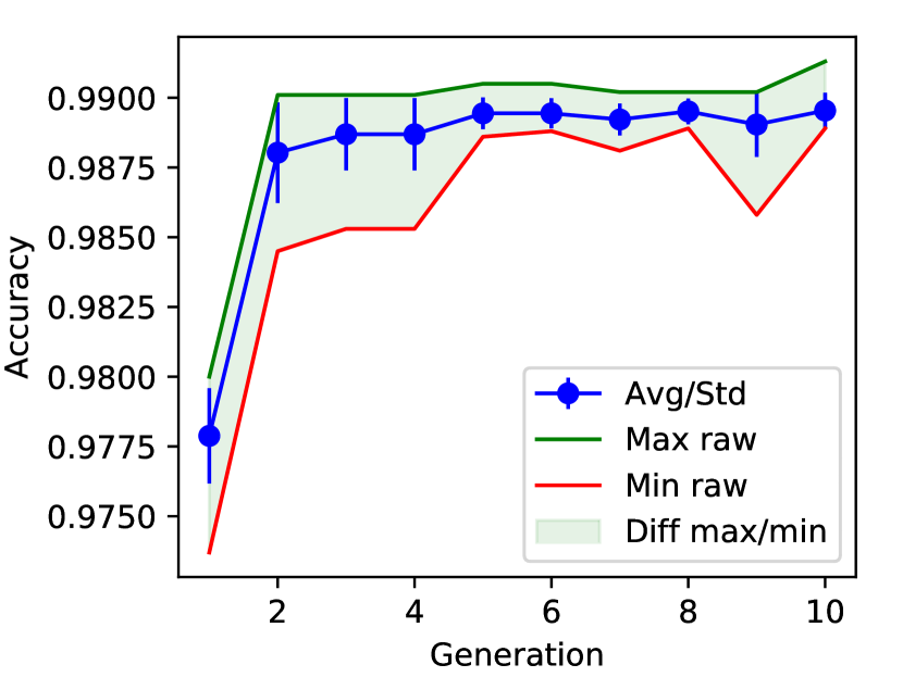
(a) Parent: Accuracy

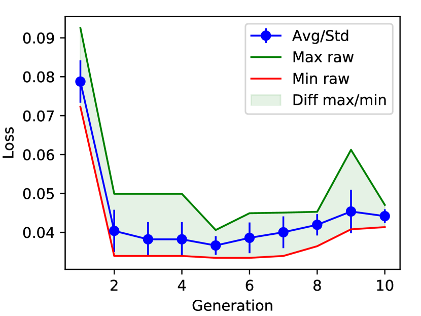
(b) Parent: Loss

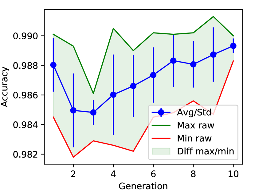
(c) Child: Accuracy

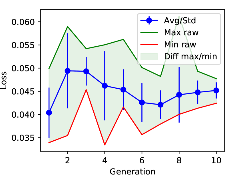
(d) Child: Loss

Figure 3: Generation Analysis of Gadam.

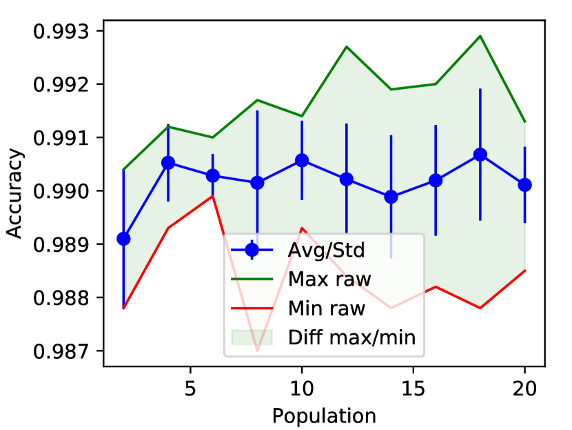
(a) Parent: Accuracy

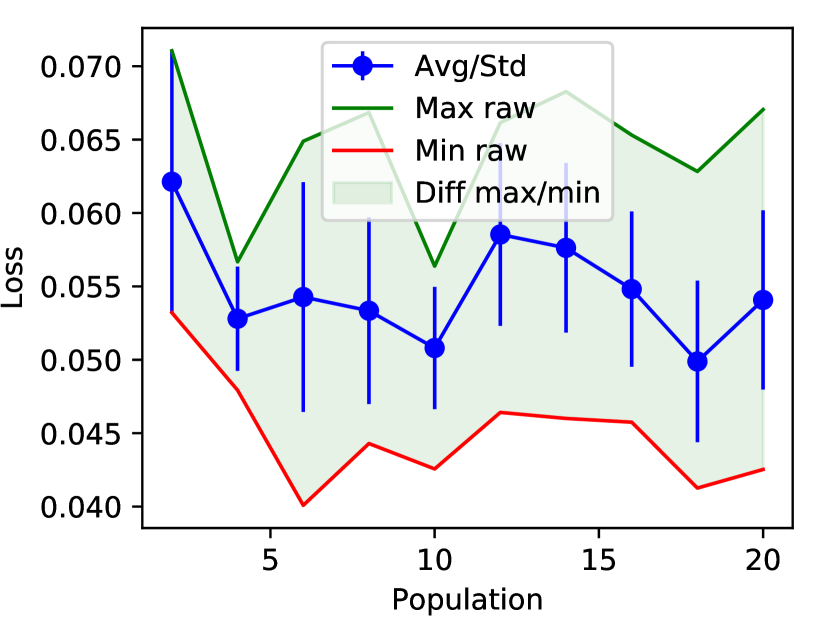
(b) Parent: Loss

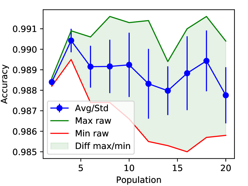
(c) Child: Accuracy

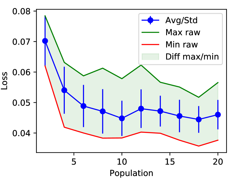
(d) Child: Loss

Figure 4: Population Analysis of Gadam.

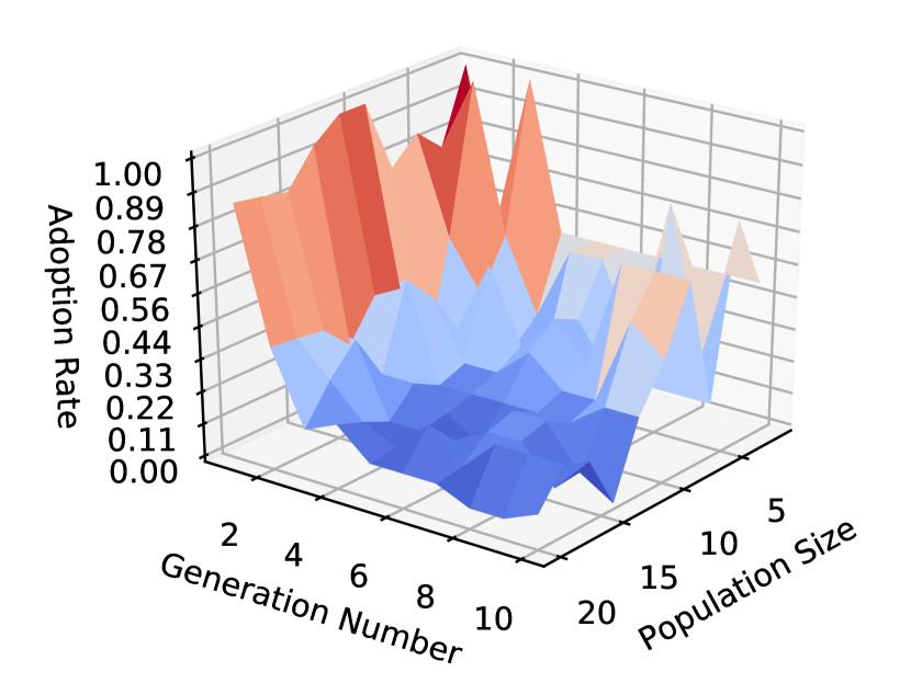
Figure 5: Child Model Adoption Rate in Different Settings.

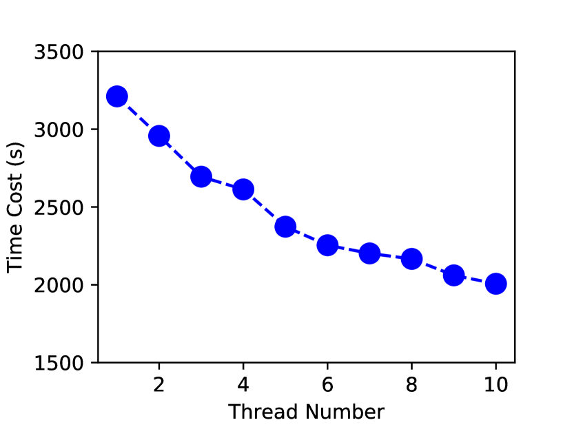
Figure 6: Learning Efficiency Analysis of Gadam on Parallel Computing Platform.

5.2 Learning Setting Analysis of Gadam

In this section, we will provide the analysis of Gadam learning setting parameters, including both the generation number and population size. In Figure 4, we provide the analysis about the generation number impact on the performance of Gadam in learning the LeNet-5 model, where the generation number is selected from $\{1,2,\cdots,10\}$. According to the results, as the generation number increases, the performance of both the parent and child models will get improved first and then remain stable. It indicates that Gadam can also achieve very fast convergence in generations. In Figure 4, we will analyze the affect of the population size parameter on the learning performance of Gadam, where the population size is selected from $\{2,4,\cdots,20\}$. According to the results, as a large population of unit models are involved in the Gadam algorithm, the average unit model learning performance of Gadam may vary slightly. Meanwhile, their standard deviation gets larger and larger, and some of the unit models will achieve very outstanding performance, which will be more likely to be selected for evolution to improve the learning performance.

Besides the learning performance of the Gadam algorithm in different settings, we are also interested in the child model adoption rate in the model evolution process, whose results are illustrated in Figure 6. According to the plot, for the Gadam algorithm at the beginning generations, the child models can generally outperform the parent model, and child model adoption rate is very high. Meanwhile, as the generation continues, the parent model will dominate the evolution process. The impact of population on the adoption rate is not significant. As illustrated in the plot, with a larger population, the unit model in Gadam may have various learning performance, while the child model adoption rate is relatively lower.

5.3 Efficiency Analysis of Gadam

In Figure 6, we study the learning efficiency of Gadam based on the parallel computing setting. Here, the experiments are carried on the Dell T630 EdgePower standalone server with 256 GB memory, 2 Intel E5-2698 CPUs (20 core/40 thread each) and Ubuntu 16.04. Among the generations, the computation is sequential and it is hard to parallelize. Therefore, in the experiments, we just need to test the intra-generation computation efficiency. We set the training epoch number as $5K$ and the unit model population as $10$, but change the number of involved threads with values in $\{1,2,\cdots,10\}$. According to the results, as more threads are used in the computing platform, the time cost used by Gadam in learning the LeNet-5 model will decrease first consistently.

5.4 Experimental Results of on Other Dataset

In Table 4, we show the performance of CNN learned with Gadam with several other baseline methods on the ORL dataset. The ORL dataset [25] contains 400 gray-scale facial images of 40 persons. Here, similar to LeNet-5, the CNN model consist of 2 convolutional layers with $16$ and $32$ feature maps of $5\times 5$ kernels, and two 2 $\times$ 2 max-pooling layers. Two full connection layers with $1024$ and $40$ hidden units will connect the convolutional layers with the output layer, where ReLU, cross-entropy and $0.5$-dropout rate are adopted. Here, 5/7/9 images for each person are randomly sampled for model training, and the results on the remaining testing images are provided in Table 4.

Table 3: Experiment Results on ORL Dataset.

Comparison Methods	Settings
	5 images	7 images	9 images
CNN (Gadam)	97.00	99.17	100.00
CNN (Adam)	96.50	97.50	98.50
gcForest	91.00	96.67	97.50
Random Forest	91.00	93.33	95.00
SVM (rbf)	80.50	82.50	85.00
kNN (k=3)	76.00	83.33	92.50

Table 4: Experiment Results on Other Datasets.

Comparison Methods	Datasets
	YEAST	ADULT	LETTER
MLP (Gadam)	63.70	87.05	96.90
MLP (Adam)	62.05	85.03	96.70
gcForest	63.45	86.40	97.40
Random Forest	60.44	85.63	96.28
SVM (rbf)	40.76	76.41	97.06
kNN (k=3)	48.80	76.00	95.23

Besides these image datasets and the CNN model, we also carried the empirical experiments on several other types of benchmark datasets and models, whose results are summarized in Table 4. The datasets used in the experiments include YEAST, ADULT and LETTER, which can be downloaded from the sites at the footnote. Here, we use MLP as the unit model to be learned with Gadam, and we also compare it with several other baseline methods. According to the results, Gadam can also learn better MLP model than Adam. Furthermore, compared with the other baseline methods, MLP (Gadam) can effectively outperform them except the LETTER dataset, where gcForest performs slightly better than MLP (Gadam).

6 Conclusion

In this paper, we have introduced a novel optimization algorithm, i.e., Gadam, which is capable to learn the variables for deep learning models both effectively and efficiently. By combining Adam and genetic algorithm together, Gadam can learn the unit models with Adam and evolve them with the genetic algorithm. At the same time, Gadam also integrates the advantages of Adam and genetic algorithm, which can converge fast, avoid sinking into the local optima, and be effectively deployable on parallel/distributed computing platforms. Extensive experiments have been done on many real-world benchmark datasets, and the experimental results show that Gadam can outperform the existing optimization algorithms in deep neural network learning in terms of both its effectiveness and efficiency.

References

- [1] E. Arisoy, T. Sainath, B. Kingsbury, and B. Ramabhadran. Deep neural network language models. In WLM, 2012.
- [2] O. E. D. and I. G. Genetic algorithms for evolving deep neural networks. In GECCO Comp ’14, 2014.
- [3] E. David and I. Greental. Genetic algorithms for evolving deep neural networks. CoRR, abs/1711.07655, 2017.
- [4] D. Decoste and B. Schölkopf. Training invariant support vector machines. Mach. Learn., 2002.
- [5] L. Deng, G. Hinton, and B. Kingsbury. New types of deep neural network learning for speech recognition and related applications: An overview. In ICASSP, 2013.
- [6] T. Dozat. Incorporating nesterov momentum into adam. In ICLR Workshop, 2016.
- [7] J. Duchi, E. Hazan, and Y. Singer. Adaptive subgradient methods for online learning and stochastic optimization. J. Mach. Learn. Res., 2011.
- [8] X. Glorot and Y. Bengio. Understanding the difficulty of training deep feedforward neural networks. In AISTATS, 2010.
- [9] I. Goodfellow, Y. Bengio, and A. Courville. Deep Learning. MIT Press, 2016. http://www.deeplearningbook.org.
- [10] G. Hinton. A practical guide to training restricted boltzmann machines. In Neural Networks: Tricks of the Trade (2nd ed.). 2012.
- [11] G. Hinton, L. Deng, D. Yu, G. Dahl, A. Mohamed, N. Jaitly, A. Senior, V. Vanhoucke, P. Nguyen, T. Sainath, and B. Kingsbury. Deep neural networks for acoustic modeling in speech recognition. IEEE Signal Processing Magazine, 2012.
- [12] G. Hinton, S. Osindero, and Y. Teh. A fast learning algorithm for deep belief nets. Neural Comput., 2006.
- [13] S. Hochreiter and J. Schmidhuber. Long short-term memory. Neural Comput., 1997.
- [14] J. Holland. Genetic algorithms. Scientific American, 1992.
- [15] H. Jaeger. Tutorial on training recurrent neural networks, covering BPPT, RTRL, EKF and the “echo state network” approach. Technical report, Fraunhofer Institute for Autonomous Intelligent Systems (AIS), 2002.
- [16] N. Keskar and R. Socher. Improving generalization performance by switching from adam to SGD. CoRR, abs/1712.07628, 2017.
- [17] D. Kingma and J. Ba. Adam: A method for stochastic optimization. CoRR, abs/1412.6980, 2014.
- [18] A. Krizhevsky, I. Sutskever, and G. Hinton. Imagenet classification with deep convolutional neural networks. In NIPS, 2012.
- [19] Y. LeCun, Y. Bengio, and G. Hinton. Deep learning. Nature, 521, 2015. http://dx.doi.org/10.1038/nature14539.
- [20] Y. Lecun, L. Bottou, Y. Bengio, and P. Haffner. Gradient-based learning applied to document recognition. Proceedings of the IEEE, 1998.
- [21] M. Mitchell. An Introduction to Genetic Algorithms. MIT Press, 1998.
- [22] A. Mnih and G. Hinton. A scalable hierarchical distributed language model. In NIPS. 2009.
- [23] H. Robbins and S. Monro. A stochastic approximation method. The annals of mathematical statistics, 1951.
- [24] R. Salakhutdinov and G. Hinton. Semantic hashing. International Journal of Approximate Reasoning, 2009.
- [25] F. Samaria and A. C. Harter. Parameterisation of a stochastic model for human face identification. In WACV, 1994.
- [26] F. Such, V. Madhavan, E. Conti, J. Lehman, K. Stanley, and J. Clune. Deep neuroevolution: Genetic algorithms are a competitive alternative for training deep neural networks for reinforcement learning. CoRR, abs/1712.06567, 2017.
- [27] I. Sutskever, J. Martens, G. Dahl, and G. Hinton. On the importance of initialization and momentum in deep learning. In ICML, 2013.
- [28] D. Thierens and D. Goldberg. Convergence models of genetic algorithm selection schemes. In Y. Davidor, H. Schwefel, and R. Männer, editors, Parallel Problem Solving from Nature — PPSN III, 1994.
- [29] T. Tieleman and G. Hinton. Lecture 6.5—RmsProp: Divide the gradient by a running average of its recent magnitude. COURSERA: Neural Networks for Machine Learning, 2012.
- [30] P. Vincent, H. Larochelle, I. Lajoie, Y. Bengio, and P. Manzagol. Stacked denoising autoencoders: Learning useful representations in a deep network with a local denoising criterion. J. Mach. Learn. Res., 2010.
- [31] J. Weston, S. Bengio, and N. Usunier. Large scale image annotation: Learning to rank with joint word-image embeddings. Journal of Machine Learning, 2010.
- [32] J. Weston, S. Bengio, and N. Usunier. Wsabie: Scaling up to large vocabulary image annotation. In IJCAI, 2011.
- [33] J. Zhang, L. Cui, and F. Gouza. segen: Sample-ensemble genetic evolutional network model. CoRR, abs/1803.08631, 2018.
- [34] Z. Zhou and J. Feng. Deep forest: Towards an alternative to deep neural networks. In IJCAI, 2017.