Tell Me Something New:
A New Framework for Asynchronous Parallel Learning

Abstract

We present a novel approach for parallel computation in the context of machine learning that we call “Tell Me Something New” (TMSN). This approach involves a set of independent workers that use broadcast to update each other when they observe “something new”. TMSN does not require synchronization or a head node and is highly resilient against failing machines or laggards. We demonstrate the utility TMSN by applying it to learning boosted trees. We show that our implementation is 10 times faster than XGBoost [1] and LightGBM [2] on the splice-site prediction problem [3, 4].

1 Introduction

Ever-larger training sets call for ever faster learning algorithms. On the other hand, computer clock rates are unlikely to increase beyond 4 GHz in the foreseeable future. As a result there is a keen interest in parallelized machine learning algorithms [5].

The most common approach to parallel ML is based on Valiant’s bulk synchronous [6] model. This approach calls for a set of workers and a master. The system works in (bulk) iterations. In each iteration the master sends a task to each worker and then waits for its response. Once all machines responded, the master proceeds to the next iteration. Thus the head node enforces synchronization (at the iteration level) and maintains a state that is shared by all of the workers.

Unfortunately, bulk synchronization does not scale well to more than 10–20 computers. Network congestion, latencies due to synchronization, laggards, and failing computers result in diminishing benefits from adding more workers to the cluster [7, 8].

There have been several attempts to break out of the bulk-synchronized framework, most notably the work of Recht et al. on Hogwild [9] and Lian et al. on asynchronous stochastic descent [10]. Hogwild significantly reduces the synchronization penalty by using asynchronous updates and parameter servers. The basic idea is to decentralize the task of maintaining a global state and relying on sparse updates to limit the frequency of update clashes.

Tell Me Something New

Our first contribution is a new approach for parallelizing ML algorithms which eliminates synchronization and the global state and instead uses a distributed policy that guarantees progress. We call this approach “Tell Me Something New” (TMSN). To explain TMSN we start with an analogy.

Consider a team of a hundred investigators that is going through thousands of documents to build a criminal case where time is of the issue. Assume also that most of the documents contain little or no new information. How should the investigators communicate their findings with each other? We contrast the bulk-synchronous (BS) approach and the TMSN approach. In the BS approach, each investigator takes a stack of documents to their cubicle and reads through it. Then all of the investigator meet in a room and tell each other what they found. Once they are done, the process repeats. One problem with this approach is that the fast readers have to wait for the slow readers. Another is that a decision needs to be made as to how many documents or pages, to put in each stack. Too many and the iterations would be very slow, too few and all of the time would be spent in meetings.

The TMSN approach is radically different. In this approach, each investigator gets documents independently according to their speed of reading and work habits. There is no meeting either. Instead, when an investigator finds a piece of information that she believes is new, she stands up in her cubicle and tells all of the other workers about it. This has several advantages: nobody is ever waiting for anybody else; the new information is broadcasted as soon as it is available, and the system is fault resilient — somebody falling asleep has little effect on the others. The analogy to parallel ML maps investigators to computers, “case” to “model”, and “new information” to “improved model”.

More concretely, TMSN for model learning works as follows. Each worker has a model $H$ and an upper bound $L$ on the true loss of $H$. The worker searches for a better model $H^{\prime}$ whose loss upper bound is $L^{\prime}$. If $L^{\prime}$ is significantly smaller than $L$, then the worker takes two actions. First, $H^{\prime},L^{\prime}$ replaces $H,L$. Second $(H^{\prime},L^{\prime})$ is broadcast to all other workers. Each worker also listens to the broadcast channel. If it receives pair $(H^{\prime},L^{\prime})$ it checks whether $L^{\prime}$ is significantly lower than its own upper bound $L$. If it is, the worker replaces $(H,L)$ with $(H^{\prime},L^{\prime})$. Otherwise, the worker discards the pair.

Boosting trees using TMSN

Our second contribution is an application of TMSN to boosted decision trees. Boosted trees is a highly effective and widely used machine learning method. In recent years there have been several implementations of boosting that greatly improve over previous implementations in terms of running time, in particular, XGBoost [1] and LightGBM [2]. These implementations scale up to training sets of many millions, or even billions of training examples. Both implementations can run in one of two configurations: a memory-only configuration where all of the training data is stored in main memory, and a memory and disk configuration where the data is on disk and is copied into memory when needed. The memory-only version is significantly faster, but require a machine with very large memory.

We present an implementation of boosting tree learning using TMSN that we call Sparrow. This is a disk and memory implementation, which requires only a fraction of the training data to be stored in memory. Yet, as our comparative experiments show, it is about 10 times faster than XGBoost and LightGBM using the memory only configuration.

The rest of the paper is divided into four sections. First we give a general description of TMSN in Section 2. Then we introduce a special application of our algorithm, namely Sparrow, in Section 3. After that we describe in more details of the algorithms and the system design of Sparrow in Section 4. Finally, we present empirical results in Section 5.

2 Tell Me Something New

We start with a general description of TMSN which will be followed by a description of TMSN for boosting. To streamline our presentation we consider binary classification, but other supervised or unsupervised learning problem can be accommodated with little change.

We are given

• A set of classifiers ${\cal H}$, each classifier $H\in{\cal H}$ is a mapping from an input space $X$ to a binary label $\{-1,+1\}$.

• A stream of labeled examples $(x_{1},y_{1}),(x_{2},y_{2}),\ldots$, $x_{i}\in X$, $y_{i}\in\{-1,+1\}$, generated IID according to a fixed but unknown distribution ${\cal D}$.

The goal of the algorithm is to find a classifier $H\in{\cal H}$ that minimized the error probability $\mbox{err}(H)\doteq P_{(x,y)\sim{\cal D}}[H(x)\neq y]$

All workers start from the same initial classifier $H_{0}$ which is improved iteratively. Some iterations end with the worker finding a better classifier by itself, others end with the worker receiving a better classifier from another worker. The sequences of classifiers corresponding to different workers can be different, but with high probability they all converge to the same classifier.

Denote each worker by an index $i=1,\ldots,n$. On iteration $t$ each worker has its current classifier $H_{i}(t)$ and a set of $m$ candidate classifiers $G_{i}^{j}(t)$. An error upper bound $\widehat{\mbox{err}}(H_{i}(t))$ is associated with $H_{i}(t)$ so that with high probability $\widehat{\mbox{err}}(H_{i}(t))\geq\mbox{err}(H_{i}(t))$.

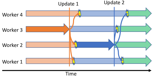
Figure 1: Execution timeline of a TMSN system System consists of four workers. The first update occurs when worker 3 identifies a better classifier $H_{1}$. It then replaces $H_{0}$ with $H_{1}$ and broadcasts $(H_{1},z_{1})$ to the other workers. The other workers receive the message the at different times, depending on network congestion. At that time they interrupt the scanner (yellow explosions) and start using $H_{1}$. Next, worker 2 identifies an improved rule $H_{2}$ and the same process ensues.

The worker reads examples from the stream and uses them to estimate the errors of the candidates. It stops when it finds a candidate that, with high probability, has an error smaller than $\widehat{\mbox{err}}(H_{i}(t))-\epsilon$ for some constant “gap” parameter $\epsilon>0$.

More precisely, the worker uses a stopping rule that chooses a stopping time and a candidate rule and has the property that, with high probability, the chosen candidate rule has an error smaller than $\widehat{\mbox{err}}(H_{i}(t))-\epsilon$. This candidate then replaces the current classifier, the new upper bound is set to be $\widehat{\mbox{err}}(H_{i}(t+1))=\widehat{\mbox{err}}(H_{i}(t))-\epsilon$, a new set of candidates is chosen and the worker proceeds to the next iteration. At the same time the worker broadcasts the pair $(H_{i}(t+1),\widehat{\mbox{err}}(H_{i}(t+1))$.

A separate process in each worker listens to broadcasts of this type. When worker $i$ receives a pair $(H,\widehat{\mbox{err}}(H))$ it compares the upper bound $\widehat{\mbox{err}}(H)$ with the upper bound associated with it’s current classifier $\widehat{\mbox{err}}(h_{i}(t))$. If $\widehat{\mbox{err}}(H)<\widehat{\mbox{err}}(h_{i}(t))-\epsilon$, it interrupts the current search and sets $H_{i}(t+1)=H$. If not the received pair is discarded.

Note that the only assumption that the workers make regarding the incoming messages is that the upper bound $\widehat{\mbox{err}}(H)$ is sound. In other words that, with hight probability, it is an upper bound on the true error $\mbox{err}(H)$. There is no synchronization and if a worker is slow or fails, the effect on the other workers is minimal.

Different implementations of TMSN differ in the way that they generate candidate classifiers and in the stopping rules that they use. For TMSN to be effective, the stopping rule should be both sound and tight. If it is not sound, then the scheme falls apart, and if it is not tight, then the stopping rules stop later than needed, slowing down convergence.

Next, we describe how TMSN is applied to boosting.

3 TMSN for Boosting

Boosting algorithms [11] are iterative, they generate a sequence of strong rules of increasing accuracy. The strong rule at iteration $T$ is a weighted majority over $T$ of the the weak rules in $\mathcal{W}$.

$$H_{T}(x)=\mbox{sign}\left(\sum_{t=1}^{T}\alpha_{t}h_{t}(x)\right)$$

For the purpose of TMSN we define ${\cal H}$ to be the set of strong rules combining any number of weak rules from $\mathcal{W}$.

Boosting algorithms can be interpreted as gradient descent algorithm [12]. Specifically, if we define the potential of the strong rule $H$ with respect to the training set ${\cal S}$ to be

$$Z_{{\cal S}}(H_{T})\doteq\frac{1}{n}\sum_{i=1}^{n}e^{-y_{i}H_{T}(x_{i})},$$

then AdaBoost is equivalent to coordinate-wise gradient descent, where the coordinates are the elements of $\mathcal{W}$. Suppose we have the strong rule $H$ and consider changing it to $H+\alpha h$ for some $h\in\mathcal{W}$ and for some small $\alpha$. The derivative of the potential wrt $\alpha$ is:

$$\left.\frac{\partial}{\partial\alpha}\right|_{\alpha=0}Z_{{\cal S}}(H+\alpha h)=\frac{1}{n}\sum_{i=1}^{n}\left.\frac{\partial}{\partial\alpha}\right|_{\alpha=0}e^{-y_{i}(H(x_{i})+\alpha h(x_{i}))}=\frac{1}{n}\sum_{i=1}^{n}-y_{i}h(x_{i})e^{-y_{i}H(x_{i})}$$

Our goal is to minimize the average potential $Z_{{\cal S}}(H_{T+1})$, therefor our goal is to find a weak rule $h$ that makes the gradient negative. Another way of expressing this goal is to find a weak rule with a large empirical edge:

$$\hat{\gamma}(h)\doteq\sum_{i=1}^{n}w_{i}y_{i}h(x_{i})\mbox{ where }w_{i}=\frac{1}{Z}e^{-y_{i}H(x_{i})};Z=\sum_{i=1}^{n}e^{-y_{i}H(x_{i})}$$ (1)

$w_{i}$ defines a distribution over the training examples, with respect to which we are measuring the correlation between $h(x_{i})$ and $y_{i}$. This is the original view of boosting, which is the process of finding weak rules with significant edges with respect to different distributions. We distinguish between the empirical edge $\hat{\gamma}(h)$, which depends on the sample, and the true edge, which depends on the underlying distribution:

$$\gamma(h)\doteq E_{(x,y)\sim{\cal D}}(w(x,y)yh(x))\mbox{ where }w(x,y)=\frac{1}{Z}{\cal D}(x,y)e^{-yH(x)}$$ (2)

and $Z$ is the normalization factor with respect the the true distribution ${\cal D}$.

A small but important observation is that boosting does not require finding the weak rule with the largest edge at each iteration. Rather, it is enough to find a rule for which we are sure that it has a significant (but not necessarily maximal) advantage. More precisely, we want to know that, with high probability over the choice of ${\cal S}\sim{\cal D}^{n}$ the rule $h$ has a significant true edge $\gamma(h)$.

Sequential Analysis and Early Stopping

The standard approach when looking for the best weak rule is to compute the error of candidate rules using all available data, and then select the rule $h$ that maximizes the empirical edge $\hat{\gamma}(h)$. However, as described above, this can be over-kill. Observe that if the true edge $\gamma(h)$ is large it can be identified as such using a small number of examples.

Bradley and Schapire [13] and Domingo and Watanabe [14] proposed using early stopping to take advantage of such situations. The idea is simple: instead of scanning through all of the training examples when searching for the next weak rule, a stopping rule is checked for each $h\in\mathcal{W}$ after each training example, and if this stopping rule “fires” then the scan is terminated and the $h$ that caused the rule to fire is added to the strong rule. We use early stopping in our algorithm.

For reasons that will be explained in the next section, we use a different stopping rule than [13] or [14]. We use a stopping rule proposed in [15] for which they prove the following

Theorem 1 (based on [15] Theorem 4)

Let $M_{t}$ be a martingale $M_{t}=\sum_{i}^{t}X_{i}$, and suppose there are constants $\{c_{k}\}_{k\geq 1}$ such that for all $i\geq 1$, $|X_{i}|\leq c_{i}$ w.p. 1. For $\forall\sigma>0$, with probability at least $1-\sigma$ we have

$$\forall t:|M_{t}|\leq C\sqrt{\left(\sum_{i=1}^{t}c_{i}^{2}\right)\left(\log\log\left(\frac{\sum_{i=1}^{t}c_{i}^{2}}{|M_{t}|}\right)+\log\frac{1}{\sigma}\right)},$$

where $C$ is a universal constant.

Effective Sample Size

Equation 2 defines $\hat{\gamma}(h)$, which is an estimate of $\gamma(h)$. How accurate is this estimate? Our initial gut reaction is that if ${\cal S}$ contains $n$ examples the error should be about $1/\sqrt{n}$. However, when the examples are weighted this is clearly wrong. Suppose, for example that $k$ out of the $n$ examples have weight one and the rest have weight zero. Obviously in this case we cannot hope for an error smaller than $1/\sqrt{k}$.

A more quantitative analysis follows. Suppose that the weights of the examples in the training set ${\cal S}=\{(x_{1},y_{1}),\ldots,(x_{n},y_{n})\}$ are $w_{1}=w(x_{1},y_{1}),\ldots,w_{n}=w(x_{n},y_{n})$. Thinking of finding a good weak rule in terms of hypothesis testing, the null hypothesis is that the weak rule $h$ has no edge. Finding a rule that is significantly better than random corresponds to rejecting the hypothesis that $\gamma(h)=0$. Assuming the null hypothesis, $y_{i}h(x_{i})$ is $+1$ with probability 1/2 and $-1$ with probability $1/2$. From central limit theorem and assuming $n$ is larger than $100$, we get that the null distribution for $\hat{\gamma}(h)=\sum_{i=1}^{n}w_{i}y_{i}h(x_{i})$ is normal with zero mean and standard deviation $\sum_{i=1}^{n}w_{i}^{2}$. The statistical test one would use in this case is the ${\mathbf{Z}}$-test for

$${\mathbf{Z}}=\frac{\hat{\gamma}(h)}{\sqrt{\sum_{i=1}^{n}w_{i}^{2}}}=\frac{\sum_{i=1}^{n}w_{i}y_{i}h(x_{i})}{\sqrt{\sum_{i=1}^{n}w_{i}^{2}}}$$ (3)

As should be expected, the value of ${\mathbf{Z}}$ remains the same whether or not $\sum_{i=1}^{n}w_{i}=1$. Based on Equation 3 we define the effective number of examples corresponding to the un-normalized weights $w_{1},\ldots,w_{n}$ as:

$${n_{\mbox{eff}}}\doteq\frac{\left(\sum_{i=1}^{n}w_{i}\right)^{2}}{\sum_{i=1}^{n}w_{i}^{2}}$$ (4)

Owen [16] used a different line of argument to arrived at a similar measure of the effective samples size for a weighted sample.

The quantity ${n_{\mbox{eff}}}$ plays a similar role in large deviation bounds such as the Hoeffding bound [17] (details ommitted). It also plays a central role in Theorem 1 and thus in the stopping rule that we use.

To understand the important role that ${n_{\mbox{eff}}}$ plays in our algorithm, supppose the training set is of size $n$ and that only $m\ll n$ examples can fit in memory. Our approach is to start by placing a random subset of size $m$ into memory and then run multiple boosting iterations using this subset. As the strong rule improves, ${n_{\mbox{eff}}}$ decreases and as a result the stopping rule based on Theorem 1 requires increasingly more examples before it is triggered. When ${n_{\mbox{eff}}}/m$ crosses a pre-specified threshold the algorithm flushes out the training examples currently in memory and samples a new set of $m$ examples using acceptance probability proportional to their weights. The new examples have uniform weights and therefor after sampling ${n_{\mbox{eff}}}=m$.

Intuitively, weighted sampling utilizes the computer’s memory better than uniform sampling because it places in memory more difficult examples and fewer easy examples. The result is better estimates of the edges of specialist weak rules that make predictions on high-weight difficult examples.

Another concern is the fraction of the examples that are selected. In the method described here the expected fraction is $(\frac{1}{n}\sum_{i=1}^{n}w_{i})/(\max_{i}w_{i})$.

4 System architecture and Algorithms

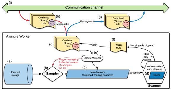
Figure 2: The Sparrow system architecture.

The Sparrow distributed system consists of a collection of independent workers connected through a shared communication channel. There is no synchronization between the workers and no identified “head node” to coordinate the workers. The result is a highly resilient system in which there is no single point of failure and the overall slowdown resulting from machine slowness or failure is proportional to the fraction of faulty machines.

Each worker is responsible for a finite (small) set of weak rules. This is a type of feature-based parallelization [18]. The worker’s task is to identify a weak rule, based on one of the features in the set, that has a significant edge.

We assume each worker stores all of the training examples on it’s local disk (element (a) in Figure 2).

Our description of Sparrow is in two parts. First, we describe the design of a single Sparrow worker. Following that, we describe how concurrent workers use the TMSN protocol to update each other. Figure 2 depicts the architecture of a single computer and its interaction with the communication channel. Pseudocode with additional detail is provided in the supplementary material to this paper.

4.1 A single Sparrow worker

As was said above, each worker is responsible for a set of the weak rules. The worker’s task is to identify a rule that has a significant edge (Equation 2). The worker consists of two subroutines that can execute in parallel: a Scanner (d) and a Sampler (b). We describe each subroutine in turn.

The Scanner

(element (d) in Figure 2) The Scanner’s task is to read training examples sequentially and stop when it has identified one of the rules to be a good rule. More specifically, at any time point the Scanner stores the current strong rule $H_{t}$, a set of candidate weak rules ${\cal W}$ (which define the candidate strong rules of TMSN) and a target edge $\gamma_{t}$. The scanner scans the training examples stored in memory sequentially, one at a time. It computes the weight of the examples using $H_{t}$ and then updates a running estimate of the edge of each weak rule $h\in{\cal W}$.

The scan stops when the stopping rule determine that the true edge of a particular weak rule $\gamma(h_{t})$ is, with high probability, larger than a threshold $\gamma$. The worker then adds the identified weak rule $h_{t}$ (f) to the current strong rule $H_{t}$ to create a new strong rule $H_{t+1}$ (g).

The worker computes a “performance score” $z_{t+1}$ which is an upper bound on the $Z$-score the strong rule by adding the weak rule to it. The pair $(H_{t+1},z_{t+1})$ is broadcast to the other workers (i). The worker then resumes it’s search using the strong rule $H_{t+1}$.

The Sampler

Our assumption is that the entire training dataset does not fit into main memory and is therefore stored in external storage (a). As boosting progresses, the weights of the examples become increasingly skewed, making the dataset in memory effectively smaller. To counteract that skew, the Sampler prepares a new training set, in which all of the examples have equal weight, by using selective sampling. When the effective number of examples associated with the old training set becomes too small, the scanner stops using the old training set and starts using the new one.

The sampler uses selective sampling by which we mean that the probability that an example $(x,y)$ is added to the sample is proportional to $w(x,y)$. Each added example is assigned an initial weight of $1$.

Incremental Updates:

Our experience shows that the most time consuming part of our algorithms is the computation of the predictions of the strong rules $H_{t}$. A natural way to reduce this computation is to perform it incrementally. In our case this is slightly more complex than in XGBoost or LightGBM, because Scanner scans only a fraction of the examples at each iteration. To implement incremental update we store for each example, whether it is on disk or in memory, the results of the latest update. Specifically, we store for each training example the tuple $(x,y,w_{s},w_{l},H_{l})$, Where $x,y$ are the feature vector and the label, $H_{l}$ is the strong rule last used to calculate the weight of the example. $w_{l}$ is the weight last calculated, and $w_{s}$ is example’s weight when it was last sampled by the sampler. In this way Scanner and Sampler share the burden of computing the weights, a cost that turns out to be the lion’s share of the total run time for our system.

4.2 Communication between workers

Communication between the workers is based on the TMSN protocol. As explained in Section 4.1, when a worker identifies a new strong rule, it broadcasts $(H_{t+1},z_{t+1})$ to all of the other workers. Where $H_{t+1}$ is the new strong rule and $z_{t+1}$ is an upper bound on the true $Z$-value of $H_{t+1}$. One can think of $z_{t+1}$ as a “certificate of quality” for $H_{t+1}$.

When a worker receives a message of the form $(H,z)$, it either accepts or rejects it. Suppose that the worker’s current strong rule is $H_{t}$ whose performance score is $z_{t}$. If $z_{t}<z$ then the worker interrupts the Scanner and restarts it with $(H_{t},z_{t})\leftarrow(H,z)$. If $z_{t}\geq z$ then $(H,z)$ is discarded and the scanner continues running uninterrupted.

5 Experiments

In this section we describe the results of experiments comparing the run time of Sparrow with those of two leading implementations of boosted trees: XGBoost and LightGBM.

Algorithm	Instance	Instance Memory	Training (minutes)
XGBoost, in-memory	x1e.xlarge	122 GB	414.6
XGBoost, off-memory	r3.xlarge	30.5 GB	1566.1
LightGBM, in-memory	x1e.xlarge	122 GB	341.6
LightGBM, off-memory	r3.xlarge	30.5 GB	449.7
TMSN, sample 10%	c3.xlarge	7.5 GB	57.4 (1 worker)
			17.7 (10 workers)

Table 1: Experiments on the Splice Site Detection Task

Setup

We use a large dataset that was used in other studies of large scale learning on detecting human acceptor splice site [3, 4]. The learning task is binary classification. We use the same training dataset of 50 M samples as in the other work, and validate the model on the testing data set of 4.6 M samples. The training dataset on disk takes over 27 GB in size.

As the code is not fully developed yet, we restrict our trees to one level so-called “decision stumps”. We plan to perform comparisons using multi-level trees and more than two labels. We expect similar runtime performance there. To generate comparable models, we also train decision stumps in XGBoost and LightGBM (by setting the maximum tree depth to 1).

Both XGBoost and LightGBM are highly optimized, and support multiple tree construction algorithms. For XGBoost, we selected approximate greedy algorithm for the efficiency purpose. LightGBM supports using sampling in the training, which they called Gradient-based One-Side Sampling (GOSS). GOSS keeps a fixed percentage of examples with large gradients, and then randomly sample from remaining examples with small gradients. We selected GOSS as the tree construction algorithm for LightGBM.

All algorithms in comparison optimize the exponential loss as defined in AdaBoost. We also evaluated the final model by calculating its area under precision-recall curve (AUPRC) on the testing dataset.

Finally, the experiments are all conducted on EC2 instances from Amazon Web Services. Since XGBoost requires 106 GB memory space for training this dataset in memory, we used instances with 120 GB memory for such setting. Detailed description of the setup is listed in Table 1.

Evaluation

Performance of each of the algorithm in terms of the exponential loss as a function of time on the testing dataset is given in Figure 3. Observe that all algorithms achieve similar final loss, but it takes them different amount of time to reach that final loss. We summarize these differences in Table 1 by using the convergence time to an almost optimal loss of $0.061$. Observe XGBoost off-memory is about 27 times slower than a single Sparrow worker which is also off-memory. That time improves by another factor of 3.2 by using 10 machines instead of 1.

In Figure 4 we perform the comparison in terms of AUPRC. The results are similar in terms of speed. However, in this case XGBoost and LightGBM ultimately achieve a slightly better AUPRC. This is baffling, because all algorithms work by minimizing exponential loss.

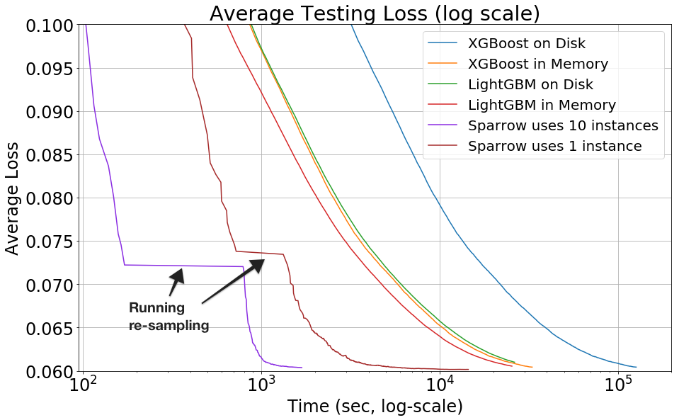
Figure 3: Comparing the average loss on the testing data using Sparrow, XGBoost, and LightGBM, lower is better. The period of time that the loss is constant for Sparrow is when the algorithm is generating a new sample set.

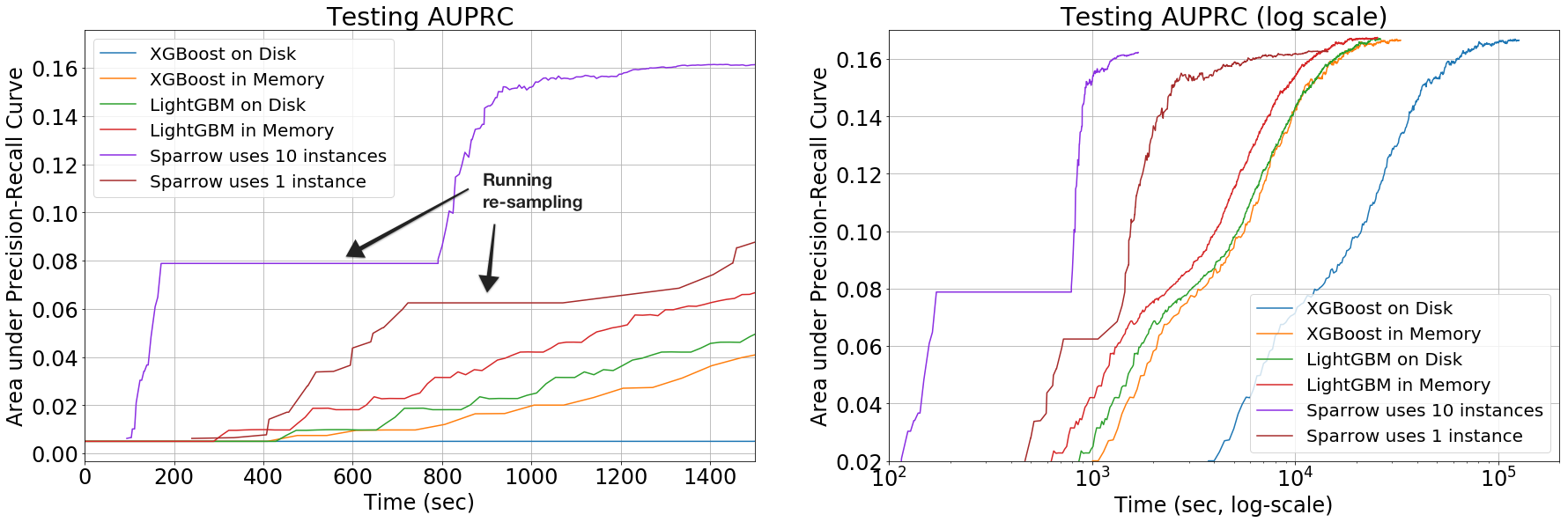
Figure 4: Comparing the area under the precision-recall curve (AUPRC) on the testing data using Sparrow, XGBoost, and LightGBM, higher is better. (left) Normal scale, clipped on right. (right) Log scale, clipped on left. The period of time that the AUPRC is constant for Sparrow is when the algorithm is generating a new sample set.

Conclusions

While the results are exciting plenty of work remains. We plan to extend the algorithm to boosting full trees as well as other types of classifiers. In addition, we observe that run time is now dominated by the time it takes to create new samples, we have some ideas for how to significantly reduce the sampling time.

Appendix

Algorithm 1 Procedures for the main algorithm and communication

Procedure MainAlgorithm

Initialize $H=0,L=0$

Create initial sample $S$ by calling Sample

for $k:=1\ldots K$ do

     $Ret\leftarrow\textsc{Scanner}(\gamma_{0},M,i,H,{\cal W})$

     if $Ret$ is Fail then

         Call Sample to Get a New Sample.

     else

         $i^{\prime},h,\gamma\leftarrow Ret$

         $i\leftarrow i^{\prime}$

         $H\leftarrow H+\frac{1}{2}\log\frac{1/2+\gamma}{1/2-\gamma}h$

         Update $L$      

Procedure Communication

(broadcasting out local models)

when $H$ is updated in this worker do

     broadcast $(H,L)$ to all other workers

(receiving remote models from others)

when received an $\left(H_{\mbox{new}},L_{\mbox{new}}\right)$ pair do

     if $L_{\mbox{new}}<L$ then

         Interrupt Scanner

         Replace $\left(H,L\right)$ with $\left(H_{\mbox{new}},L_{\mbox{new}}\right)$

         Restart Scanner

     else

         Discard $\left(H_{\mbox{new}},L_{\mbox{new}}\right)$      

Algorithm 2 Functions for the Scanner and Sampler

In-memory sampled set $S$ is defined globally

function Scanner($\gamma_{0},M,i_{0},H,{\cal W}$)

     $\gamma\leftarrow\gamma_{0},m\leftarrow 0,i\leftarrow i_{0}$

     $V\leftarrow 0,W\leftarrow 0$

     $\forall h\in{\cal W}:m[h]=0$

     while True do

         $(x,y,w_{s},w_{l},H_{l})\leftarrow S[i]$

         $i\leftarrow(i+1)\mbox{ mod }|S|$

         if $i=i_{0}$ then

              return Fail          

         $m\leftarrow m+1$

         if $m>M$ then

              $\gamma\leftarrow\gamma/2$, $m\leftarrow 0$          

         $w\leftarrow\textsc{UpdateWeight}($

                   $x,y,w_{l},H_{l},w_{s},H,i)$

         $V\leftarrow V+w^{2}$, $W\leftarrow W+|w|$

         for all $h\in{\cal W}$ do

              $m[h]\leftarrow m[h]+wyh(x)$

              $ret\leftarrow\textsc{StoppingRule}($

                            $W,V,m[h],\gamma)$

              if $ret=\textbf{True}$ then

                  return $i,h,\gamma$                             

function UpdateWeight($x,y,w_{l},H_{l},w_{s},H,i$)

     Calculate score update $s\leftarrow H(x)-H_{l}(x)$

     Calculate new weight $w\leftarrow w_{l}\exp{(ys)}$

     Update Sample: $S[i]=(x,y,w_{s},w,H)$

     return $w/w_{s}$

function StoppingRule($W,V,m,\gamma$)

     $C,\delta$ are global parameters.

     $M\leftarrow|m-2\gamma W|$

     return $M>C\sqrt{V(\log\log{V\over M_{0}}+\log{1\over\delta}}$

function Sample

     Input: Randomly permuted, disk-resident training-set.

     Input Current model $H$

     $S\leftarrow\{\}$

     for all  available training data $(x,y)$  do

         $w_{s}\leftarrow\exp{(-yH(x))}$

         With the probability proportional to $w_{s}$,

              $S\leftarrow S+\{(x,y,w_{s},w_{s},H)\}$.      

     return S

References

- [1] Tianqi Chen and Carlos Guestrin. XGBoost: A Scalable Tree Boosting System. In Proceedings of the 22Nd ACM SIGKDD International Conference on Knowledge Discovery and Data Mining, KDD ’16, pages 785–794, New York, NY, USA, 2016. ACM.
- [2] Guolin Ke, Qi Meng, Thomas Finley, Taifeng Wang, Wei Chen, Weidong Ma, Qiwei Ye, and Tie-Yan Liu. LightGBM: A Highly Efficient Gradient Boosting Decision Tree. In I. Guyon, U. V. Luxburg, S. Bengio, H. Wallach, R. Fergus, S. Vishwanathan, and R. Garnett, editors, Advances in Neural Information Processing Systems 30, pages 3146–3154. Curran Associates, Inc., 2017.
- [3] Soeren Sonnenburg and Vojtěch Franc. COFFIN: A Computational Framework for Linear SVMs. In Proceedings of the 27th International Conference on International Conference on Machine Learning, ICML’10, pages 999–1006, USA, 2010. Omnipress.
- [4] Alekh Agarwal, Oliveier Chapelle, Miroslav Dudík, and John Langford. A Reliable Effective Terascale Linear Learning System. Journal of Machine Learning Research, 15:1111–1133, 2014.
- [5] Ron Bekkerman, Mikhail Bilenko, and John Langford. Scaling Up Machine Learning: Parallel and Distributed Approaches. Cambridge University Press, 2012. Google-Books-ID: c5v5USMvcMYC.
- [6] Leslie G. Valiant. A Bridging Model for Parallel Computation. Commun. ACM, 33(8):103–111, August 1990.
- [7] Matei Zaharia, Reynold S. Xin, Patrick Wendell, Tathagata Das, Michael Armbrust, Ankur Dave, Xiangrui Meng, Josh Rosen, Shivaram Venkataraman, Michael J. Franklin, Ali Ghodsi, Joseph Gonzalez, Scott Shenker, and Ion Stoica. Apache Spark: A Unified Engine for Big Data Processing. Commun. ACM, 59(11):56–65, October 2016.
- [8] Frank McSherry, Michael Isard, and Derek G. Murray. Scalability! But at what COST? In 15th Workshop on Hot Topics in Operating Systems (HotOS XV), Kartause Ittingen, Switzerland, 2015. USENIX Association.
- [9] Benjamin Recht, Christopher Re, Stephen Wright, and Feng Niu. Hogwild: A Lock-Free Approach to Parallelizing Stochastic Gradient Descent. In J. Shawe-Taylor, R. S. Zemel, P. L. Bartlett, F. Pereira, and K. Q. Weinberger, editors, Advances in Neural Information Processing Systems 24, pages 693–701. Curran Associates, Inc., 2011.
- [10] Xiangru Lian, Yijun Huang, Yuncheng Li, and Ji Liu. Asynchronous Parallel Stochastic Gradient for Nonconvex Optimization. In C. Cortes, N. D. Lawrence, D. D. Lee, M. Sugiyama, and R. Garnett, editors, Advances in Neural Information Processing Systems 28, pages 2737–2745. Curran Associates, Inc., 2015.
- [11] Robert E. Schapire and Yoav Freund. Boosting: Foundations and Algorithms. MIT Press, 2012. Google-Books-ID: blSReLACtToC.
- [12] Llew Mason, Jonathan Baxter, Peter Bartlett, and Marcus Frean. Boosting Algorithms As Gradient Descent. In Proceedings of the 12th International Conference on Neural Information Processing Systems, NIPS’99, pages 512–518, Cambridge, MA, USA, 1999. MIT Press.
- [13] Joseph K. Bradley and Robert E. Schapire. FilterBoost: Regression and Classification on Large Datasets. In Proceedings of the 20th International Conference on Neural Information Processing Systems, NIPS’07, pages 185–192, USA, 2007. Curran Associates Inc.
- [14] Carlos Domingo and Osamu Watanabe. Scaling Up a Boosting-Based Learner via Adaptive Sampling. In Knowledge Discovery and Data Mining. Current Issues and New Applications, Lecture Notes in Computer Science, pages 317–328. Springer, Berlin, Heidelberg, April 2000.
- [15] Akshay Balsubramani. Sharp Finite-Time Iterated-Logarithm Martingale Concentration. arXiv:1405.2639 [cs, math, stat], May 2014. arXiv: 1405.2639.
- [16] Art B. Owen. Monte Carlo Theory, Methods and Examples. 2013.
- [17] Wassily Hoeffding. Probability Inequalities for Sums of Bounded Random Variables. Journal of the American Statistical Association, 58(301):13–30, 1963.
- [18] Doina Caragea, Adrian Silvescu, and Vasant Honavar. A Framework for Learning from Distributed Data Using Sufficient Statistics and Its Application to Learning Decision Trees. International Journal of Hybrid Intelligent Systems, 1(1-2):80–89, January 2004.
- [19] Genshiro Kitagawa. Monte Carlo Filter and Smoother for Non-Gaussian Nonlinear State Space Models. Journal of Computational and Graphical Statistics, 5(1):1–25, 1996.