Optimal DR-Submodular Maximization and Applications to Provable Mean Field Inference

Abstract

Mean field inference in probabilistic models is generally a highly nonconvex problem. Existing optimization methods, e.g., coordinate ascent algorithms, can only generate local optima.

In this work we propose provable mean field methods for probabilistic log-submodular models and its posterior agreement (PA) with strong approximation guarantees. The main algorithmic technique is a new Double Greedy scheme, termed DR-DoubleGreedy, for continuous DR-submodular maximization with box-constraints. This one-pass algorithm achieves the optimal 1/2 approximation ratio, which may be of independent interest. We validate the superior performance of our algorithms with baseline results on both synthetic and real-world datasets.

1 Introduction

Consider the following scenario: You want to build a recommender system for $n$ products to sell. Let $\mathcal{V}$ contain all the products. The system is expected to recommend a subset of products $S\subseteq\mathcal{V}$ to the user. This recommendation should reflect relevance and diversity of the user’s choice, such that it will raise the readiness to buy. The two most important components in building such a system are (1) learning a utility function $F(S)$, which measures the utility of any subset of products, and (2) inference, i.e., finding the subset $\Omega^{*}$ with the highest utility given the learnt function $F(S)$. The above task can be achieved using a class of probabilistic graphical models that devise a distribution on all subsets of $\mathcal{V}$. Such a distribution is known as a point process. Specifically, it defines $p(S)\propto\exp(F(S))$, which renders subset of products $S$ with high utility to be very likely suggested. In general, inference in point processes is #P-hard. One resorts to approximate inference methods via either variational techniques [39] or sampling.

In this paper we develop mean field methods with provable guarantees. Both of the two components in the recommender system example above can be achieved via provable mean field methods since (i) the latter provide approximate inference given a utility function and, (ii) by using proper differentiation techniques, the iterative process of mean field approximation can be unrolled to serve as a differentiable layer [41], thus enabling the backpropagation of the training error to parameters of $F(S)$. Thereby, learning $F(S)$ in an end-to-end fashion can utilize modern deep learning and stochastic optimization techniques.

The most important property which we require on $F(S)$ is submodularity, which naturally models relevance and diversity. Djolonga et al. [14] have used submodular functions $F(S)$ to define two classes of point processes: $p(S)\propto\exp(F(S))$ is termed probabilistic log-submodular models, while $p(S)\propto\exp(-F(S))$ is called probabilistic log-supermodular models. They are strict generalizations of classical point processes, such as DPPs [29]. The variational techniques from Djolonga & Krause [14]; Djolonga et al. [16] focus on giving tractable upper bounds of the log-partition functions. This work provides provable lower bounds through mean field approximation, which also completes the picture of variational inference for probabilistic submodular models (PSMs).

The most frequently used algorithm for mean field approximation is the CoordinateAscent algorithm. It maximizes the ELBO objective in a coordinate-wise manner. CoordinateAscent has been shown to reach stationary points/local optima. However, local optima may be arbitrarily poor, as we demonstrate in §​ A, and CoordinateAscent would get stuck in these poor local optima without extra techniques, which motivates our pursuit to develop provable methods.

We firstly investigate the properties of mean field approximation for probabilistic log-submodular models, and show that it falls into a general class of nonconvex problem, called continuous DR-submodular maximization with box-constraints. Continuous submodular optimization is a class of well-behaved nonconvex programs, which has attracted increasingly more attention recently. Then we propose a new one-epoch algorithm for this general class of nonconvex problem, called DR-DoubleGreedy. It achieves the optimal $1/2$ approximation ratio in linear time. Lastly, we extend one-epoch algorithms to multiple epochs, resulting in provable mean field algorithms, termed DG-MeanField.

Typical Application Domains. Recommender systems are just one illustrating example. There are numerous scenarios that can benefit from the mean field method in this work. These settings include, but not limited to, existing applications of submodular models, such as diversity models [37; 16], experimental design using approximate submodular objectives [2], variable selection [28], data summarization [30], dictionary learning [26] etc. Another category of applications is conducting model validation using information-theoretic criteria. In order to infer the hyperparamters in the model $F(S)$, practitioners do validation by splitting the training data into multiple folds, and then train models on them. Posterior-Agreement (PA, [7; 5]) provides an information-theoretic criterion for the models trained on these folds, to measure the fitness of one specific hyperparameter configuration. We show in §​ 2.1 that PA can be efficiently approximated by the techniques developed in this work.

Contributions.

Motivated by the broad applicability of mean field approximation, we contribute in the following respects: i) We propose the first optimal algorithm for the general problem of continuous DR-submodular maximization with box-constraints, which runs in linear time. ii) Based on the optimal algorithm, we propose provable mean field approaches for probabilistic log-submodular models and its PA. iii) We also present efficient polynomial methods to evaluate the multilinear extensions for a large category of practical objectives, which are used for optimizing the mean field objectives.

1.1 Problem Statement and Related Work

Notation. Boldface letters, e.g. $\mathbf{x}$, represent vectors. Boldface capital letters, e.g. $\mathbf{A}$, denote matrices. $x_{i}$ is the $i^{\text{th}}$ entry of $\mathbf{x}$, $A_{ij}$ the $(ij)^{\text{th}}$ entry of $\mathbf{A}$. We use $\mathbf{e}_{i}$ to denote the standard $i^{\text{th}}$ basis vector. $f(\cdot)$ is used to specify a continuous function, and $F(\cdot)$ to represent a set function. $[n]:=\{1,...,n\}$. Given two vectors $\mathbf{x},\mathbf{y}$, $\mathbf{x}\leq\mathbf{y}$ means $\forall i,\,x_{i}\leq y_{i}$. $\mathbf{x}\vee\mathbf{y}$ and $\mathbf{x}\wedge\mathbf{y}$ is defined as coordinate-wise maximum and coordinate-wise minimum, respectively. Finally, $\mathbf{x}|_{i}k$ is the operation of setting the $i^{\text{th}}$ entry of $\mathbf{x}$ to $k$, while keeping all the others unchanged, i.e., $\mathbf{x}|_{i}k=\mathbf{x}-x_{i}\mathbf{e}_{i}+k\mathbf{e}_{i}$.

All of the mean field approximation problems investigated in this work fall into the following nonconvex maximization problem:

$$\underset{{\mathbf{x}\in[\mathbf{a},\;\mathbf{b}]}}{{\text{maximize}}}\;\;f(\mathbf{x}),$$ (P)

where $f:{\cal X}\rightarrow{\mathbb{R}}$ is continuous DR-submodular, ${\cal X}=\prod_{i=1}^{n}{\cal X}_{i}$, each ${\cal X}_{i}$ is an interval [1; 3]. Continuous DR-submodular functions define a subclass of continuous submodular functions with the additional diminishing returns (DR) property: $\forall\mathbf{a}\leq\mathbf{b}\in{\cal X}$, $\forall i\in[n],\forall k\in{\mathbb{R}}_{+}$ it holds $f(k\mathbf{e}_{i}+\mathbf{a})-f(\mathbf{a})\geq f(k\mathbf{e}_{i}+\mathbf{b})-f(\mathbf{b})$. If $f$ is differentiable, DR-submodularity is equivalent to $\nabla f$ being an antitone mapping from ${\mathbb{R}}^{n}$ to ${\mathbb{R}}^{n}$. If $f$ is twice-differentiable, DR-submodularity is equivalent to all of the entries of $\nabla^{2}f(\mathbf{x})$ being non-positive. A function $f$ is DR-supermodular iff $-f$ is DR-submodular.

Background & Related Work. Submodularity is one of the most important properties in combinatorial optimization and many applications for machine learning, with strong implications for both guaranteed minimization and approximate maximization in polynomial time [27]. Continuous extensions of submodular set functions play an important role in submodular optimization, representative instances include Lovász extension [32], multilinear extension [9; 38; 11; 12] and the softmax extension for DPPs [19]. These guaranteed optimizations have been advanced to continuous domains recently, for both minimization [1; 36] and maximization [3; 4; 40; 13; 33]. Specifically, Bach [1] studies continuous submodular minimization without constraints. He also discusses the possibility of using the technique for mean field inference of probabilistic log-supermodular models. [3; 4] characterize continuous submodularity using the DR property and propose provable algorithms for maximization.

Most related to this work is the classical problem of unconstrained submodular maximization (USMs), which has been studied in binary [6], integer [35] and continuous domains [3]. For the general problem P, at first glance one may consider discretization-based methods: Discretizing the continous domain and transform P to be an integer optimization problem, then solve it using the reduction [17] or the integer Double Greedy algorithm [35]. However, discretization-based methods are not practical for P: Firstly discretization will inevitably introduce errors for the original continuous problem P; Secondly, the computational cost is too high. Thus we turn to continuous methods. The shrunken Frank-Wolfe in [4] provides $1/e$ approximation guarantee and sublinear rate of convergence for P, but it is still computationally too expensive: In each iteration it has to calculate the full gradient, which costs $n$ times as much as computing a partial derivative.

Based on the above analysis, the most promising algorithm to consider would be the Double Greedy algorithm [3], which needs to solve $\mathcal{O}\!\left(n\right)$ 1-D subproblems, and achieves $1/3$ guarantee for continuous submodular maximization. Since it only needs $f(\mathbf{x})$ to be continuous submodular, we call it Submodular-DoubleGreedy in the sequel. In this work we propose a new Double Greedy scheme, achieving the optimal $1/2$ approximation ratio of P.

Posterior-Agreement (PA) is developed as an information-theoretic criterion for model selection [21] and algorithmic validation [23; 5]. It originates from the approximation set coding framework proposed by [7]. Recently, [8] prove rigorous asymptotics of PA on two typical combinatorial problems: Sparse minimum bisection and Lawler’s quadratic assignment problem. [14; 15] study variational inference for PSMs, they propose L-Field to give upper bounds for log-supermodular models through optimizing the subdifferentials. However, they did not give tractable lower bounds for probabilistic log-submodular models.

Along with the development of this work, [34] proposed an optimal algorithm for DR-submodular maximization. Their algorithm (Algorithm 4 in [34], termed BSCB: Binary-Search Continuous Bi-greedy) needs to estimate the partial derivative of the objective, which is not needed in our algorithm. Furthermore, our algorithm is arguably easier to interpret and implement than BSCB. We did extensive experiments (see §​ 5 for details on experimental statistics) to compare them, the results show that both algorithms generate promising solutions, however, our algorithm produces better solutions than BSCB in most of the experiments.

2 Applications to Mean Field Approximation

Mean field inference aims to approximate the intractable distribution $p(S)\propto\exp(F(S))$ by a fully factorized surrogate distribution $q(S|{\mathbf{x}}):=\prod_{i\in S}x_{i}\prod_{j\notin S}(1-x_{j}),\mathbf{x}\in[0,1]^{n}$. This can be achieved by maximizing the (ELBO) objective, which provides a lower bound for the log-partition function, $\text{(ELBO)}\leq\log\text{Z}=\log\sum_{S\subseteq\mathcal{V}}\exp(F(S))$. Specifically, the optimization problem is,

$$\max_{\mathbf{x}\in[\mathbf{0},\mathbf{1}]}f(\mathbf{x}) :=\overbrace{{\mathbb{E}}_{q(S|\mathbf{x})}[F(S)]}^{\text{multilinear extension of }F(S):f_{\text{mt}}(\mathbf{x})}$$

$$-\sum\nolimits_{i=1}^{n}[x_{i}\log x_{i}+(1-x_{i})\log(1-x_{i})]$$

$$\;=f_{\text{mt}}(\mathbf{x})+\sum\nolimits_{i\in\mathcal{V}}H(x_{i}),\quad\text{({\color[rgb]{0.6015625,0,0}ELBO})}$$ (1)

where $H(x_{i}):=-[x_{i}\log x_{i}+(1-x_{i})\log(1-x_{i})]$ is the binary entropy function and by default $0\log 0=0$. $f_{\text{mt}}(\mathbf{x}):={\mathbb{E}}_{q(S|\mathbf{x})}[F(S)]$ is the multilinear extension [10] of $F(S)$. The above (ELBO) is continuous DR-submodular w.r.t. $\mathbf{x}$, thus falling into the general problem class P. At first glance, $f_{\text{mt}}(\mathbf{x})$ seems to require an exponential number of operations for evaluation; we show in §​ 4 that $f_{\text{mt}}(\mathbf{x})$ and its gradients can be computed precisely in polynomial time for many classes of practical objectives, such as facility location, FLID [37], set cover [31] and graph cuts. Maximizing (ELBO) to optimality provides the tightest lower bound of $\log\text{Z}$ in terms of the KL divergence $\mathbb{KL}(q\|p)$. We put details in §​ C.

In addition to the traditional mean field objective (ELBO) in 1, here we further formulate a second class of mean field objectives. They come from Posterior-Agreement (PA) for probabilistic log-submodular models, which is an information-theoretic criterion to conduct model and algorithmic validation [7; 8; 5].

2.1 Mean Field Inference of Posterior-Agreement (PA)

Let us again consider the recommender example: usually there are some hyperparameters in the model/utility function $F(S)$ that require adaptation to the input data. One natural way to do so is through model validation: Split the training data into multiple folds, train a model on each fold D one would infer a “noisy” posterior distribution $p(S|\text{D})$. PA measures the agreement between these “noisy” posterior distributions.

Assume w.l.o.g. that there are two folds of data $\text{D}^{\prime},\text{D}^{\prime\prime}$ in the sequel. In the PA framework, we have two consecutive targets: 1) Direct inference based on the two posterior distributions $p(S|\text{D}^{\prime})$ and $p(S|\text{D}^{\prime\prime})$. This task amounts to find the MAP solution of the PA distribution (which is discussed in the next paragraph), it can be approximated by standard mean field inference. 2) Use the PA objective 3 as a criterion for model validation/selection. Since in general the PA objective 3 is intractable, we will still use mean field lower bounds and some upper bounds in [14] to provide estimations for it.

Mean Field Approximation of the Posterior-Agreement Distribution. A probabilistic log-submodular model is a special case of a Gibbs random field with unit temperature and $-F(S)$ as the energy function. In PA framework, we explicitly keep $\beta$ as the inverse temperature, $p_{\beta}(S|\text{D}):=\frac{\exp(\beta F(S|\text{D}))}{\sum_{\tilde{S}\subseteq\mathcal{V}}\exp(\beta F(\tilde{S}|\text{D}))},\forall S\subseteq\mathcal{V}$, where D is the dataset used to train the model $F(S|\text{D})$. The PA distribution is defined as,

$$p^{\text{PA}}(S)\propto p_{\beta}(S|\text{D}^{\prime})p_{\beta}(S|\text{D}^{\prime\prime})\propto\exp[\beta(F(S|\text{D}^{\prime})+F(S|\text{D}^{\prime\prime}))].$$

Note that its log partition function is still intractable. In order to approximate $p^{\text{PA}}(S)$, we use mean field approximation with a surrogate distribution $q(S|{\mathbf{x}}):=\prod_{i\in S}x_{i}\prod_{j\notin S}(1-x_{j})$,

$$\log\text{Z}^{\text{PA}}=\log\sum\nolimits_{S\subseteq\mathcal{V}}\exp[\beta(F(S|\text{D}^{\prime})+F(S|\text{D}^{\prime\prime}))]$$

$$\geq\beta\ \mathbb{E}_{q(S|{\mathbf{x}})}[F(S|\text{D}^{\prime})]+\beta\ \mathbb{E}_{q(S|{\mathbf{x}})}[F(S|\text{D}^{\prime\prime})]$$ (2)

$$\quad+\sum\nolimits_{i\in\mathcal{V}}H(x_{i}).\quad\quad\qquad\qquad\qquad\text{({\color[rgb]{0.6015625,0,0}PA-ELBO})}$$

Maximizing (PA-ELBO) in 2 still falls into the general problem class P (see §​ C for details). Maximizing (PA-ELBO) also serves as a building block for the second target below.

Lower Bounds for the Posterior-Agreement Objective. The PA objective is used to measure the agreement between the two posterior distributions motivated by an information-theoretic analogy [8; 5]. By introducing the same surrogate distribution $q(S|\mathbf{x})$, one can easily derive that,

$$\mathrm{log}\sum\nolimits_{S\subseteq\mathcal{V}}p_{\beta}(S|\text{D}^{\prime})p_{\beta}(S|\text{D}^{\prime\prime})\quad\text{(PA\ objective)}$$ (3)

$$\!\!\!\!\!\!\geq\underbrace{{\mathbb{H}}(q)\!+\!\beta\ {{\mathbb{E}}}_{q}F(S|\text{D}^{\prime})\!+\!\beta\ {{\mathbb{E}}}_{q}F(S|\text{D}^{\prime\prime})}_{\text{(PA-ELBO) in \lx@cref{refnum}{pa_elbo}}}$$

$$-\log\text{Z}(\beta;\text{D}^{\prime})-\log\text{Z}(\beta;\text{D}^{\prime\prime})$$

where ${\mathbb{H}}(q)$ is the entropy of $q$, $\text{Z}(\beta;\text{D}^{\prime})$ and $\text{Z}(\beta;\text{D}^{\prime\prime})$ are the partition functions of the two noisy distributions, respectively. In order to find the best lower bound for PA, one need to maximize w.r.t. $q(S|\mathbf{x})$ the (PA-ELBO) objective, at the same time, find the upper bounds for $\log\text{Z}(\beta;\text{D}^{\prime})+\log\text{Z}(\beta;\text{D}^{\prime\prime})$. The latter can be achieved using techniques from [14]. We summarize the details in §​ D to make it self-contained.

3 An Optimal Algorithm for Continuous DR-Submodular Maximization

Unfortunately, problem P is generally hard: The $1/2$ hardness result [3, Proposition 5] can be easily translated to P with details deferred to §​ B.1. The following question arises naturally: Is it possible to achieve the optimal $1/2$ approximation ratio (unless RP=NP) by properly utilizing the extra DR propety in P? To affirmatively answer this question, we propose a new Double Greedy algorithm for continuous DR-submodular maximization called DR-DoubleGreedy and prove a $1/2$ approximation ratio.

3.1 A Deterministic $1/2$-Approximation for Continuous DR-Submodular Maximization

Input: $\max_{\mathbf{x}\in[\mathbf{a},\mathbf{b}]}f(\mathbf{x})$, $f(\mathbf{x})$ is DR-submodular, $[\mathbf{a},\mathbf{b}]\subseteq{\cal X}$

1 $\mathbf{x}^{0}\leftarrow\mathbf{a}$, $\mathbf{y}^{0}\leftarrow\mathbf{b}$;

2 for $k=1\rightarrow n$ do

3       let $v_{k}$ be the coordinate being operated;

4       find $u_{a}$ such that $f(\mathbf{x}^{k-1}|_{v_{k}}u_{a})\geq\max_{u^{\prime}}f(\mathbf{x}^{k-1}|_{v_{k}}u^{\prime})-\frac{\delta}{n}$,

5      $\delta_{a}\leftarrow f(\mathbf{x}^{k-1}|_{v_{k}}u_{a})-f(\mathbf{x}^{k-1}$) ;

6      

7      find $u_{b}$ such that $f(\mathbf{y}^{k-1}|_{v_{k}}u_{b})\geq\max_{u^{\prime}}f(\mathbf{y}^{k-1}|_{v_{k}}u^{\prime})-\frac{\delta}{n}$,

8      $\delta_{b}\leftarrow f(\mathbf{y}^{k-1}|_{v_{k}}u_{b})-f(\mathbf{y}^{k-1})$ ;

9      

      $\mathbf{x}^{k}\leftarrow\mathbf{x}^{k-1}|_{v_{k}}(\frac{\delta_{a}}{\delta_{a}+\delta_{b}}u_{a}+\frac{\delta_{b}}{\delta_{a}+\delta_{b}}u_{b})$;

        // update $v_{k}^{\text{th}}$ coordinate to be a convex combination of $u_{a}$ & $u_{b}$

10      

11      $\mathbf{y}^{k}\leftarrow\mathbf{y}^{k-1}|_{v_{k}}(\frac{\delta_{a}}{\delta_{a}+\delta_{b}}u_{a}+\frac{\delta_{b}}{\delta_{a}+\delta_{b}}u_{b})$;

12      

Output: $\mathbf{x}^{n}$ or $\mathbf{y}^{n}\;(\mathbf{x}^{n}=\mathbf{y}^{n})$

Algorithm 1 DR-DoubleGreedy$(f,\mathbf{a},\mathbf{b})$

The pseudocode of DR-DoubleGreedy as summarized in Alg. 1 describes a one-epoch algorithm, sweeping over the $n$ coordinates in one pass. Like the previous Double Greedy algorithms, the procedure maintains two solutions $\mathbf{x},\mathbf{y}$, that are initialized as the lower bound $\mathbf{a}$ and the upper bound $\mathbf{b}$, respectively. In iteration $k$, it operates on coordinate $v_{k}$, and solves the two 1-D subproblems $\max_{u^{\prime}}f(\mathbf{x}^{k-1}|_{v_{k}}u^{\prime})$ and $\max_{u^{\prime}}f(\mathbf{y}^{k-1}|_{v_{k}}u^{\prime})$, based on $\mathbf{x}^{k-1}$ and $\mathbf{y}^{k-1}$, respectively. It also allows solving 1-D subproblems approximately with additive error $\delta\geq 0$ ($\delta=0$ recovers the error-free case). Let $u_{a}$ and $u_{b}$ be the solutions of these 1-D subproblems.

Unlike previous Double Greedy algorithms, we change coordinate $v_{k}$ of $\mathbf{x}^{k-1}$ and $\mathbf{y}^{k-1}$ to be a convex combination of $u_{a}$ and $u_{b}$, weighted by respective gains $\delta_{a}$, $\delta_{b}$. This convex combination is the key step that utilizes the DR property of $f$, and it also plays a crucial role in the proof.

Note that the 1-D subproblem has a closed-form solution for ELBO 1 (and similarly for PA-ELBO 2). For coordinate $i$, the partial derivative of the multilinear extension is $\nabla_{i}f_{\text{mt}}(\mathbf{x})$, and for the entropy term, it is $\nabla H(x_{i})=\log\frac{1-x_{i}}{x_{i}}$. Then $x_{i}$ should be updated as $x_{i}\leftarrow\sigma(\nabla_{i}f_{\text{mt}}(\mathbf{x}))=\bigl{(}1+\exp(-\nabla_{i}f_{\text{mt}}(\mathbf{x})\bigr{)}^{-1}$, where $\sigma$ is the logistic sigmoid function.

Theorem 1.

Assume the optimal solution of $\max_{\mathbf{x}\in[\mathbf{a},\mathbf{b}]}f(\mathbf{x})$ is $\mathbf{x}^{*}$, then for Alg. 1 it holds,

$$f(\mathbf{x}^{n})\geq\frac{1}{2}f(\mathbf{x}^{*})+\frac{1}{4}[f(\mathbf{a})+f(\mathbf{b})]-\frac{5\delta}{4}.$$ (4)

Proof Sketch. The high level proof strategy is to bound the change of an intermediate variable $\mathbf{o}^{k}:=(\mathbf{x}^{*}\vee\mathbf{x}^{k})\wedge\mathbf{y}^{k}$ through the course of Alg. 1, which is the common framework in the analysis of all existing Double Greedy variants [6; 22; 3; 35]. The novelty of our method results from the update of $\mathbf{x}$, $\mathbf{y}$, which plays a key role in achieving the optimal $1/2$ approximation ratio. Furthermore, in the analysis we find a way to utilize the DR property directly, resulting in a succinct proof. We document the details in §​ B.2, and summarize a sketch here. Firstly, using DR-submodularity, we prove that in each iteration, if we were to flip the 1-D subproblem solutions of $\mathbf{x}$ and $\mathbf{y}$, it still does not decrease the function value (in the error-free case $\delta=0$).

Lemma 1.

For all $k=1,...,n$, it holds that,

$$f(\mathbf{x}^{k-1}|_{v_{k}}u_{b})-f(\mathbf{x}^{k-1})\geq-{\delta}/{n},$$ (5)

$$f(\mathbf{y}^{k-1}|_{v_{k}}u_{a})-f(\mathbf{y}^{k-1})\geq-{\delta}/{n}.$$

Then using the new update rule and the DR property, we show that the loss on intermediate variables $f(\mathbf{o}^{k-1})-f(\mathbf{o}^{k})$ can be upper bounded by the increase of the objective value in $\mathbf{x}$ and $\mathbf{y}$ times $1/2$.

Lemma 2.

For all $k=1,...,n$, it holds that,

$$f(\mathbf{o}^{k-1})-f(\mathbf{o}^{k})$$ (6)

$$\leq \frac{1}{2}\left[f(\mathbf{x}^{k})-f(\mathbf{x}^{k-1})+f(\mathbf{y}^{k})-f(\mathbf{y}^{k-1})\right]+\frac{2.5\delta}{n}.$$

Given Lemma 2, let us sum for $k=1,...,n$. After rearrangement it reaches the final conclusion.

3.2 Multi-epoch Extensions

Though DR-DoubleGreedy reaches the optimal $1/2$ guarantee with one epoch, in practice it usually helps to use its output as an initializer, and continue optimizing coordinate-wisely for additional epochs. Since each step of coordinate update will never decrease the function value, the approximation guarantees will hold. We call this class of algorithms DoubleGreedy-MeanField, abbreviated as DG-MeanField, and summarize the pseudocode in Alg. 2.

Input: $\max_{\mathbf{x}\in[\mathbf{a},\mathbf{b}]}f(\mathbf{x})$, e.g., from the ELBO 1 or PA-ELBO 2 objective

1 Option I: DG-MeanField-$1/3$: run Submodular-DoubleGreedy [3] to get a ${1}/{3}$ initializer $\hat{\mathbf{x}}$

2Option II: DG-MeanField-$1/2$: run DR-DoubleGreedy to get a $1/2$ initializer $\hat{\mathbf{x}}$ ;

3 beginning with $\hat{\mathbf{x}}$, optimize $f(\mathbf{x})$ coordinate by coordinate for $T$ epochs ;

Algorithm 2 DG-MeanField-$1/2$ & DG-MeanField-$1/3$

4 Efficient Methods for Calculating Multilinear Extension & Gradients

In this section we present guaranteed methods to efficiently calculate the multilinear extension $f_{\text{mt}}(\mathbf{x})$ and its gradients in polynomial time. Remember that the multilinear extension is the expected value of $F(S)$ under the surrogate distribution: $f_{\text{mt}}(\mathbf{x}):={\mathbb{E}}_{q(S|\mathbf{x})}[F(S)]=\sum_{S\subseteq\mathcal{V}}F(S)\prod_{i\in S}x_{i}\prod_{j\notin S}(1-x_{j}).$ One can verify that the partial derivative of $f_{\text{mt}}(\mathbf{x})$ is,

$$\nabla_{i}f_{\text{mt}}(\mathbf{x}) ={\mathbb{E}}_{q(S|\mathbf{x},x_{i}=1)}[F(S)]-{\mathbb{E}}_{q(S|\mathbf{x},x_{i}=0)}[F(S)]$$

$$=f_{\text{mt}}(\mathbf{x}|_{i}1)-f_{\text{mt}}(\mathbf{x}|_{i}0)$$

$$=\sum_{S\subseteq\mathcal{V},S\ni i}F(S)\prod_{j\in S\backslash\{i\}}x_{j}\prod_{j^{\prime}\notin S}(1-x_{j^{\prime}})$$

$$\quad-\sum_{S\subseteq\mathcal{V}\backslash\{i\}}\ F(S)\prod_{j\in S}x_{j}\prod_{j^{\prime}\notin S,j^{\prime}\neq i}(1-x_{j^{\prime}}).$$

4.1 Gibbs Random Fields with Finite Order of Interactions

Let us use $\mathbf{v}\in\{0,1\}^{\mathcal{V}}$ to equivalently denote the $n$ binary random variables. $F(\mathbf{v})$ corresponds to the negative energy function in Gibbs random fields. If the energy function is parameterized with a finite order of interactions, i.e., $F(\mathbf{v})=\sum_{s\in\mathcal{V}}\theta_{s}v_{s}+\sum_{(s,t)\in\mathcal{V}\times\mathcal{V}}\theta_{s,t}v_{s}v_{t}+...+\sum_{(s_{1},s_{2},...,s_{d})}\theta_{s_{1},s_{2},...,s_{d}}v_{s_{1}}\cdots v_{s_{d}},\;d<\infty$, then one can verify that its multilinear extension has the following closed form,

$$f_{\text{mt}}(\mathbf{x})=\sum_{s\in\mathcal{V}}\theta_{s}x_{s}+\sum_{(s,t)\in\mathcal{V}\times\mathcal{V}}\theta_{s,t}x_{s}x_{t}+...$$ (7)

$$+\sum_{(s_{1},s_{2},...,s_{d})}\theta_{s_{1},s_{2},...,s_{d}}x_{s_{1}}\cdots x_{s_{d}}\,.$$

The gradient of this expression can also be easily derived. Given this observation, one can quickly derive the multilinear extensions of a large category of energy functions of Gibbs random fields, e.g., graph cut, hypergraph cut, Ising models, etc. Details are in §​ E.

4.2 Facility Location & FLID (Facility Location Diversity)

FLID is a diversity model [37] that has been designed as a computationally efficient alternative to DPPs. It is in a more general form than facility location. Let $\mathbf{W}\in{\mathbb{R}}_{+}^{|\mathcal{V}|\times D}$ be the weights, each row correponds to the latent representation of an item, with $D$ as the dimensionality. Then

$$F(S):= \sum\nolimits_{i\in S}u_{i}+\sum\nolimits_{d=1}^{D}(\max_{i\in S}W_{i,d}-\sum\nolimits_{i\in S}W_{i,d})$$

$$= \sum\nolimits_{i\in S}u^{\prime}_{i}+\sum\nolimits_{d=1}^{D}\max_{i\in S}W_{i,d},$$ (8)

which models both coverage and diversity, and $u^{\prime}_{i}=u_{i}-\sum_{d=1}^{D}W_{i,d}$. If $u^{\prime}_{i}=0$, one recovers the facility location objective. The computational complexity of evaluating its partition function is $\mathcal{O}\!\left(|\mathcal{V}|^{D+1}\right)$ [37], which is exponential in terms of $D$.

We now show the technique such that $f_{\text{mt}}(\mathbf{x})$ and $\nabla_{i}f_{\text{mt}}(\mathbf{x})$ can be evaluated in $\mathcal{O}\!\left(Dn^{2}\right)$ time. Firstly, for one $d\in[D]$, let us sort $W_{i,d}$ such that $W_{i_{d}(1),d}\leq W_{i_{d}(2),d}\leq\cdots\leq W_{i_{d}(n),d}$. After this sorting, there are $D$ permutations to record: $i_{d}(l),l=1,...,n,\forall d\in[D]$. Now, one can verify that,

$$f_{\text{mt}}(\mathbf{x})$$

$$=\sum_{i\in[n]}u^{\prime}_{i}x_{i}+\sum_{d}\sum_{S\subseteq\mathcal{V}}\max_{i\in S}W_{i,d}\prod_{m\in S}x_{m}\prod_{m^{\prime}\notin S}(1-x_{m^{\prime}})$$

$$=\sum_{i\in[n]}u^{\prime}_{i}x_{i}+\sum_{d}\sum_{l=1}^{n}W_{i_{d}(l),d}x_{i_{d}(l)}\prod_{m=l+1}^{n}[1-x_{i_{d}(m)}].$$

Sorting costs $\mathcal{O}\!\left(Dn\log n\right)$, and from the above expression, one can see that the cost of evaluating $f_{\text{mt}}(\mathbf{x})$ is $\mathcal{O}\!\left(Dn^{2}\right)$. By the relation that $\nabla_{i}f_{\text{mt}}(\mathbf{x})=f_{\text{mt}}(\mathbf{x}|_{i}1)-f_{\text{mt}}(\mathbf{x}|_{i}0)$, the cost is also $\mathcal{O}\!\left(Dn^{2}\right)$. For $\nabla_{i}f_{\text{mt}}(\mathbf{x})$, there exists a refined way to calculate this derivative, which we explain in §​ E.

4.3 Set Cover Functions

Suppose there are $|C|=\{c_{1},...,c_{|C|}\}$ concepts, and $n$ items in $\mathcal{V}$. Give a set $S\subseteq\mathcal{V}$, $\Gamma(S)$ denotes the set of concepts covered by $S$. Given a modular function $\mathbf{m}:2^{C}\mapsto{\mathbb{R}}_{+}$, the set cover function is defined as $F(S)=\mathbf{m}(\Gamma(S))$. This function models coverage in maximization, and also the notion of complexity in minimization problems [31]. Let us define an inverse map $\Gamma^{-1}$, such that for each concept $c$, $\Gamma^{-1}(c)$ denotes the set of items $v$ such that $\Gamma^{-1}(c)\ni v$. So the multilinear extension is,

$$f_{\text{mt}}(\mathbf{x}) =\sum\nolimits_{i\in\mathcal{V}}\mathbf{m}(\Gamma(S))\prod\nolimits_{m\in S}x_{m}\prod\nolimits_{m^{\prime}\notin S}(1-x_{m^{\prime}})$$

$$=\sum\nolimits_{c\in C}m_{c}\left[1-\prod\nolimits_{i\in\Gamma^{-1}(c)}(1-x_{i})\right].$$ (9)

The last equality is achieved by considering the situations where a concept $c$ is covered. One can observe that both $f_{\text{mt}}(\mathbf{x})$ and $\nabla_{i}f_{\text{mt}}(\mathbf{x})$ can be evaluated in $\mathcal{O}\!\left(n|C|\right)$ time.

4.4 General Case: Approximation by Sampling

In the most general case, one may only have access to the function values of $F(S)$. In this scenario, one can use a polynomial number of sample steps to estimate $f_{\text{mt}}(\mathbf{x})$ and its gradients. Specifically: 1) Sample $k$ times $S\sim q(S|\mathbf{x})$ and evaluate function values for them, resulting in $F(S_{1}),...,F(S_{k})$. 2) Return the average $\frac{1}{k}\sum_{i=1}^{k}F(S_{i})$. According to the Hoeffding bound [24], one can easily derive that $\frac{1}{k}\sum_{i=1}^{k}F(S_{i})$ is arbitrarily close to $f_{\text{mt}}(\mathbf{x})$ with increasingly more samples: With probability at least $1-\exp(-k\epsilon^{2}/2)$, it holds that $|\frac{1}{k}\sum_{i=1}^{k}F(S_{i})-f_{\text{mt}}(\mathbf{x})|\leq\epsilon\max_{S}|F(S)|$, for all $\epsilon>0$.

5 Experiments

The objectives under investigation are ELBO 1 and PA-ELBO 2 (We set $\beta=1$ in PA-ELBO). We tested on the representative FLID model on the following algorithms and baselines:

The first category is one-epoch algorithms, including \footnotesize1⃝ Submodular-DoubleGreedy from [3] with $1/3$ guarantee, \footnotesize2⃝ BSCB (Algorithm 4 in [34], termed Binary-Search Continuous Bi-greedy, where we chose $\epsilon=10^{-3}$) with $1/2$ guarantee and \footnotesize3⃝ DR-DoubleGreedy (Alg. 1) with $1/2$ guarantee.

The second category contain multiple-epoch algorithms: \footnotesize4⃝ CoordinateAscent-0: initialized as $\mathbf{0}$ and coordinate-wisely improving the solution; CoordinateAscent-1: initialized as $\mathbf{1}$; CoordinateAscent-Random: initialized as a uniform vector $U(\mathbf{0},\mathbf{1})$. \footnotesize5⃝ DG-MeanField-${1}/{3}$. \footnotesize6⃝ DG-MeanField-${1}/{2}$ from Alg. 2. \footnotesize7⃝ BSCB-Multiepoch, which is the multi-epoch extension of BSCB: After the first epoch of running BSCB, it continues to improve the solution coordinate-wisely. For all algorithms, we use the same random order to process the coordinates within each epoch.

Table 1: Summary of results on ELBO objective 1 and PA-ELBO objective 2. Sub-DG stands for Submodular-DoubleGreedy, DR-DG stands for DR-DoubleGreedy. Boldface numbers indicate the best mean of function values returned. For ELBO, the mean and standard deviation were calculated for 10 FLID models trained on 10 folds of the data. For PA-ELBO, the mean and standard deviation were calculated for models trained over $45$ pairs of folds. More details are in the experimental section.

		ELBO objective 1			PA-ELBO objective 2
Category	$D$	Sub-DG	BSCB	DR-DG	Sub-DG	BSCB	DR-DG
furniture	2	2.078$\pm$0.091	2.771$\pm$0.123	3.035$\pm$0.059	0.918$\pm$0.768	2.287$\pm$0.399	2.402$\pm$0.159
	3	1.835$\pm$0.156	2.842$\pm$0.128	3.026$\pm$0.099	1.296$\pm$1.176	2.536$\pm$0.439	2.693$\pm$0.181
$n$=32	10	1.375$\pm$0.194	2.951$\pm$0.161	2.917$\pm$0.103	1.504$\pm$1.110	2.764$\pm$0.405	2.882$\pm$0.248
carseats	2	2.089$\pm$0.166	2.863$\pm$0.090	3.045$\pm$0.069	1.015$\pm$1.081	2.106$\pm$0.228	2.348$\pm$0.219
	3	1.890$\pm$0.146	3.003$\pm$0.110	3.138$\pm$0.082	1.309$\pm$1.218	2.414$\pm$0.267	2.707$\pm$0.208
$n$=34	10	1.390$\pm$0.232	3.100$\pm$0.140	3.003$\pm$0.157	1.599$\pm$1.317	2.684$\pm$0.271	2.915$\pm$0.250
safety	2	1.934$\pm$0.402	2.727$\pm$0.212	2.896$\pm$0.098	1.370$\pm$1.203	2.049$\pm$0.280	2.341$\pm$0.161
	3	1.867$\pm$0.453	2.830$\pm$0.191	2.970$\pm$0.110	1.706$\pm$1.296	2.288$\pm$0.297	2.619$\pm$0.167
$n$=36	10	1.546$\pm$0.606	2.916$\pm$0.191	2.920$\pm$0.149	1.948$\pm$1.353	2.467$\pm$0.270	2.738$\pm$0.187
strollers	2	2.042$\pm$0.181	2.829$\pm$0.144	2.928$\pm$0.060	0.865$\pm$0.952	1.933$\pm$0.256	2.202$\pm$0.226
	3	1.814$\pm$0.264	2.958$\pm$0.146	2.978$\pm$0.077	1.172$\pm$1.063	2.181$\pm$0.297	2.543$\pm$0.254
$n$=40	10	1.328$\pm$0.544	3.065$\pm$0.162	2.910$\pm$0.140	1.702$\pm$1.334	2.480$\pm$0.304	2.767$\pm$0.336
media	2	3.221$\pm$0.066	3.309$\pm$0.055	3.493$\pm$0.051	0.372$\pm$0.286	1.477$\pm$0.128	1.336$\pm$0.101
	3	3.276$\pm$0.082	3.492$\pm$0.083	3.712$\pm$0.079	0.418$\pm$0.366	1.736$\pm$0.177	1.762$\pm$0.095
$n$=58	10	2.840$\pm$0.183	3.894$\pm$0.122	3.924$\pm$0.114	0.653$\pm$0.727	2.309$\pm$0.244	2.524$\pm$0.130
health	2	3.197$\pm$0.067	3.174$\pm$0.074	3.516$\pm$0.043	0.548$\pm$0.282	1.655$\pm$0.122	1.650$\pm$0.073
	3	3.231$\pm$0.055	3.306$\pm$0.108	3.707$\pm$0.064	0.649$\pm$0.413	1.903$\pm$0.173	2.025$\pm$0.083
$n$=62	10	2.633$\pm$0.115	3.508$\pm$0.120	3.675$\pm$0.110	0.768$\pm$0.628	2.233$\pm$0.196	2.375$\pm$0.101
toys	2	3.543$\pm$0.047	3.454$\pm$0.091	3.856$\pm$0.044	0.597$\pm$0.480	1.731$\pm$0.182	1.761$\pm$0.133
	3	3.362$\pm$0.055	3.412$\pm$0.070	3.736$\pm$0.051	0.578$\pm$0.520	1.738$\pm$0.192	1.802$\pm$0.151
$n$=62	10	3.037$\pm$0.138	3.706$\pm$0.108	3.859$\pm$0.119	0.758$\pm$0.871	2.140$\pm$0.242	2.330$\pm$0.177
diaper	2	3.500$\pm$0.058	3.517$\pm$0.058	3.636$\pm$0.043	0.295$\pm$0.158	1.119$\pm$0.063	0.665$\pm$0.116
	3	3.739$\pm$0.080	3.753$\pm$0.065	3.974$\pm$0.065	0.337$\pm$0.240	1.429$\pm$0.111	1.141$\pm$0.120
$n$=100	10	3.423$\pm$0.110	4.150$\pm$0.120	4.203$\pm$0.086	0.386$\pm$0.504	1.969$\pm$0.201	2.009$\pm$0.199
feeding	2	3.942$\pm$0.041	3.808$\pm$0.024	3.970$\pm$0.036	0.393$\pm$0.034	0.894$\pm$0.022	0.501$\pm$0.029
	3	4.333$\pm$0.031	4.095$\pm$0.032	4.390$\pm$0.031	0.503$\pm$0.072	1.232$\pm$0.041	0.893$\pm$0.046
$n$=100	10	4.611$\pm$0.053	4.553$\pm$0.079	4.860$\pm$0.056	0.608$\pm$0.239	1.808$\pm$0.087	1.820$\pm$0.078
gear	2	3.311$\pm$0.046	3.150$\pm$0.037	3.430$\pm$0.040	0.232$\pm$0.068	1.019$\pm$0.048	0.590$\pm$0.043
	3	3.538$\pm$0.048	3.347$\pm$0.045	3.721$\pm$0.050	0.303$\pm$0.132	1.257$\pm$0.085	1.020$\pm$0.064
$n$=100	10	3.065$\pm$0.083	3.550$\pm$0.050	3.670$\pm$0.067	0.312$\pm$0.232	1.566$\pm$0.130	1.514$\pm$0.072
bedding	2	3.406$\pm$0.080	3.374$\pm$0.088	3.620$\pm$0.062	0.525$\pm$0.121	1.932$\pm$0.194	2.001$\pm$0.080
	3	3.648$\pm$0.106	3.564$\pm$0.083	3.876$\pm$0.081	2.499$\pm$0.972	2.250$\pm$0.269	2.624$\pm$0.066
$n$=100	10	3.355$\pm$0.161	3.799$\pm$0.144	3.912$\pm$0.082	3.919$\pm$0.045	2.578$\pm$0.358	3.157$\pm$0.091
apparel	2	3.560$\pm$0.094	3.527$\pm$0.046	3.784$\pm$0.059	0.268$\pm$0.109	1.552$\pm$0.141	1.513$\pm$0.191
	3	3.878$\pm$0.092	3.755$\pm$0.062	4.140$\pm$0.063	0.490$\pm$0.677	1.900$\pm$0.237	2.225$\pm$0.136
$n$=100	10	3.751$\pm$0.087	4.084$\pm$0.075	4.425$\pm$0.066	0.820$\pm$1.372	2.351$\pm$0.337	2.967$\pm$0.150
bath	2	2.957$\pm$0.087	3.024$\pm$0.032	3.198$\pm$0.056	0.197$\pm$0.090	1.101$\pm$0.083	0.795$\pm$0.078
	3	3.062$\pm$0.085	3.195$\pm$0.058	3.448$\pm$0.058	0.247$\pm$0.163	1.368$\pm$0.134	1.269$\pm$0.059
$n$=100	10	2.497$\pm$0.135	3.426$\pm$0.076	3.438$\pm$0.089	0.327$\pm$0.312	1.711$\pm$0.183	1.742$\pm$0.098

We are trying to understand: 1) In terms of continuous DR-submodular maximization, how good are the solutions returned by one-epoch algorithms? 2) How good are the realized lower bounds? For small scale problems we can calculate the true log-partitions exhaustively, which servers as a natural upper bound of ELBO. All algorithms and subroutines are implemented in Python3, and source code will be released soon.

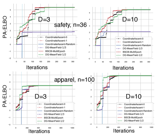
Figure 1: PA-ELBO on Amazon data. The figures trace trajectories of multi-epoch algorithms. Cyan vertical line shows the one-epoch point.

Real-world Dataset. We tested the mean field methods on the trained FLID models from [37] on Amazon Baby Registries dataset. After preprocessing, this dataset has 13 categories, e.g., “feeding” & “furniture”. One category contains a certain number of registries over the ground set of this category, e.g., “strollers” has 5,175 registries with $n=40$. One can refer to Table 1 for specific dimensionalities on each of the category. For each category, three classes of models were trained, with latent dimensions $D=2,3,10$, repectively, on 10 folds of the data.

5.1 Results on One-epoch Algorithms

Table 1 summarizes the outputs of one-epoch algorithms for both ELBO and PA-ELBO objectives. For each category, the results of FLID models with three dimensionalities ($D=2,3,10$) are reported.

ELBO Objective.

The results are summarized in columns 3 to 5 in Table 1. The mean and standard deviation are calculated for 10 FLID models trained on 10 folds of the data. One can observe that both DR-DoubleGreedy and BSCB improve over the baseline Submodular-DoubleGreedy, which has only a 1/3 approximation guarantee. Furthermore, DR-DoubleGreedy generates better solutions than BSCB for almost all of the cases, though they have the same approximation guarantee.

PA-ELBO objective.

The results are summarized in columns 6 to 8 in Table 1. For each category, out of the 10 folds of data, we have ${10\choose 2}=45$ pairs of folds. The mean and standard deviation are computed for these $45$ pairs for each category and each latent dimensonality $D$. One can still observe that DR-DoubleGreedy and BSCB significantly improve over Submodular-DoubleGreedy. Moreover, DR-DoubleGreedy produces better solutions than BSCB in most of the experiments.

5.2 Results on Multi-epoch Algorithms

PA-ELBO Objective.

Figure 1 shows representative results on PA-ELBO objectives. One can see that after one epoch, DG-MeanField-$1/2$ almost always returns the best solution. In most of the experiments, DG-MeanField-$1/2$ was the fastest algorithm to converge. However, CoordinateAscent is quite sensitive to initializations. After sufficiently many iterations, most multi-epoch algorithms converge to similar ELBO values. This is consistent with the intuition since after one epoch, all algorithms are using the same strategy: conducting coordinate-wise maximization. However, for CoordinateAscent with unlucky initializations, e.g., for category “safety” (row 1), it may get stuck in poor local optima.

The results on ELBO objectives are put into §​ F.1.

6 Conclusions

Probabilistic structured models play an eminent role in machine learning today, especially models with submodular costs. Validating such models and their parameters remains an open issue in applications. We have proposed provable mean field algorithms for probabilistic log-submodular models and their posterior agreement score. A novel Double Greedy scheme with optimal $1/2$ approximation ratio for the general problem of box-constrained continuous DR-submodular maximization has been proposed and analyzed on real-world data. We plan to generalize the guaranteed mean field approaches to probabilistic graphical models with a larger class of energy functions.

Acknowledgments

YAB would like to thank Nico Gorbach and Josip Djolonga for fruitful discussions, to thank Sebastian Tschiatschek for sharing the source code and data. This research was partially supported by the Max Planck ETH Center for Learning System

Appendix

Appendix A There Exist Poor Local Optima

If one only assume the objective function $f(\mathbf{x})$ to be continuous DR-submodular, and considering that the multilinear extension of a submodular set function is continuous DR-submodular, we can take the examples from literatures on combinatorial optimization, e.g., [18], to show that bad local optima exist.

Here we provide a stronger example, where we assume that the objective function $f(\mathbf{x})$ has the same structure as the ELBO objective 1. And still there exist bad local optima. These local optima have arbitrarily small objective value compared to the global optimum. And CoordinateAscent will get stuck in this local optimum without extra techniques.

Suppose that we have a directed graph $G=(\mathcal{V},A)$ with four vertices, $\mathcal{V}=\{1,2,3,4\}$ and four arcs, $A=\{(1,2),(2,3),(3,2),(3,4)\}$. The weights of the arcs are (let $b,c$ be large positive numbers): $w_{1,2}=c$, $w_{2,3}=c$, $w_{3,4}=c$, $w_{3,2}=bc$. Let $F(S)$ denote the sum of weights of arcs leaving $S$. Consider its ELBO (using techniques from §​ 4.1),

$$f(\mathbf{x}) =f_{\text{mt}}(\mathbf{x})+\sum_{i\in\mathcal{V}}H(x_{i})$$ (10)

$$=\sum_{(i,j)\in A}w_{ij}x_{i}(1-x_{j})+\sum_{i\in\mathcal{V}}H(x_{i})$$ (11)

$$=cx_{1}(1-x_{2})+cx_{2}(1-x_{3})+cx_{3}(1-x_{4})+bcx_{3}(1-x_{2})+\sum_{i\in\mathcal{V}}H(x_{i}).$$ (12)

Consider the point $\mathbf{y}=[0.5,1,0,0.5]^{\top}$, it has function value $f(\mathbf{y})=c+2\log 2$. Consider a second point $\bar{\mathbf{x}}=[1,0,1,0]^{\top}$, while the global optimum $f(\mathbf{x}^{\star})$ must be greater than $f(\bar{\mathbf{x}})=(2+b)c$. When $b$ becomes large, the ratio $\frac{f(\mathbf{y})}{f(\mathbf{x}^{\star})}\leq\frac{c+2\log 2}{(2+b)c}$ can be arbitrarily small.

CoordinateAscent may get stuck on the point $\mathbf{y}=[0.5,1,0,0.5]^{\top}$. This can be illustrated by considering the course of CoordinateAscent. Suppose wlog. that CoordinateAscent processes coordinates in the order of $1\rightarrow 4$ (actually it is the same with any orders).

For coordinate 1, $\nabla_{1}f_{\text{mt}}(\mathbf{x})=c(1-x_{2})$, so $\nabla_{1}f_{\text{mt}}(\mathbf{y})=0$, after applying $\sigma(\nabla_{1}f_{\text{mt}}(\mathbf{y}))$, $y_{1}$ remains to be $0.5$.

For coordinate 2, $\nabla_{2}f_{\text{mt}}(\mathbf{x})=c(1-x_{3})-bcx_{3}$, so $\nabla_{2}f_{\text{mt}}(\mathbf{y})=c$. When $c$ is sufficiently large (approaching infinity), after applying $\sigma(\nabla_{2}f_{\text{mt}}(\mathbf{y}))$, $y_{2}$ will still be 1.

For coordinate 3, $\nabla_{3}f_{\text{mt}}(\mathbf{x})=-cx_{2}+c(1-x_{4})+bc(1-x_{2})$, so $\nabla_{3}f_{\text{mt}}(\mathbf{y})=-0.5c$. When $c$ is sufficiently large (approaching infinity), after applying $\sigma(\nabla_{3}f_{\text{mt}}(\mathbf{y}))$, $y_{3}$ will still be 0.

For coordinate 4, $\nabla_{4}f_{\text{mt}}(\mathbf{x})=-cx_{3}$, so $\nabla_{4}f_{\text{mt}}(\mathbf{y})=0$, after applying $\sigma(\nabla_{4}f_{\text{mt}}(\mathbf{y}))$, $y_{4}$ remains to be $0.5$.

Appendix B Proofs for DR-DoubleGreedy

B.1 Hardness of Problem P

Observation 1.

The problem of maximizing a generally non-monotone DR-submodular continuous function subject to box-constraints is NP-hard. Furthermore, there is no $(1/2+\epsilon)$-approximation for any $\epsilon>0$, unless RP = NP.

The proof is very similar to the that of [3, Proposition 5], so we just briefly explain here. One observation is that the multilinear extension of a submodular set function is also continuous DR-submodular, so we can use the same reduction as in [3, Proposition 5] to prove the hardness results as above.

B.2 Detailed Proof of Theorem 1

See 1

Proof of Theorem 1.

Define $\mathbf{o}^{k}:=(\mathbf{x}^{*}\vee\mathbf{x}^{k})\wedge\mathbf{y}^{k}$. It is clear that $\mathbf{o}^{0}=\mathbf{x}^{*}$ and $\mathbf{o}^{n}=\mathbf{x}^{n}=\mathbf{y}^{n}$. One can notice that as Alg. 1 progresses, $\mathbf{o}^{k}$ moves from $\mathbf{x}^{*}$ to $\mathbf{x}^{n}$ (or $\mathbf{y}^{n}$).

Let $r_{a}=\frac{\delta_{a}}{\delta_{a}+\delta_{b}},r_{b}=1-r_{a}$, $u=r_{a}u_{a}+(1-r_{a})u_{b}$.

See 1

Proof of Lemma 1.

One can observe that $\mathbf{x}^{k-1}\leq\mathbf{y}^{k-1}$, so from DR-submodularity: $f(\mathbf{x}^{k-1}|_{v_{k}}u_{b})-f(\mathbf{x}^{k-1})\geq f(\mathbf{y}^{k-1}|_{v_{k}}u_{b})-f(\mathbf{y}^{k-1}|_{v_{k}}a_{v_{k}})\geq-\frac{\delta}{n}$.

Similarly, because of $\mathbf{x}^{k-1}\leq\mathbf{y}^{k-1}$ and $u_{a}\leq b_{v_{k}}$, from DR-submodularity: $f(\mathbf{y}^{k-1}|_{v_{k}}u_{a})-f(\mathbf{y}^{k-1})\geq f(\mathbf{x}^{k-1}|_{v_{k}}u_{a})-f(\mathbf{x}^{k-1}|_{v_{k}}b_{v_{k}})\geq-\frac{\delta}{n}$. ∎

See 2

Proof of Lemma 2.

Step I:

Let us try to lower bound the RHS of Lemma 2.

$$f(\mathbf{x}^{k})-f(\mathbf{x}^{k-1}) =f(\mathbf{x}^{k-1}|_{v_{k}}r_{a}u_{a}+r_{b}u_{b})-f(\mathbf{x}^{k-1})$$

$$\overset{\footnotesize1⃝}{\geq}r_{a}f(\mathbf{x}^{k-1}|_{v_{k}}u_{a})+r_{b}f(\mathbf{x}^{k-1}|_{v_{k}}u_{b})-f(\mathbf{x}^{k-1})$$

$$=r_{a}[f(\mathbf{x}^{k-1}|_{v_{k}}u_{a})-f(\mathbf{x}^{k-1})]+r_{b}[f(\mathbf{x}^{k-1}|_{v_{k}}u_{b})-f(\mathbf{x}^{k-1})]$$

$$\overset{\footnotesize2⃝}{\geq}r_{a}\delta_{a}-r_{b}\frac{\delta}{n},$$

where \footnotesize1⃝ is because of that $f$ is concave along one coordinate, \footnotesize2⃝ is from Lemma 1.

Similarly,

$$f(\mathbf{y}^{k})-f(\mathbf{y}^{k-1}) =f(\mathbf{y}^{k-1}|_{v_{k}}r_{a}u_{a}+r_{b}u_{b})-f(\mathbf{y}^{k-1})$$

$$\geq r_{a}f(\mathbf{y}^{k-1}|_{v_{k}}u_{a})+r_{b}f(\mathbf{y}^{k-1}|_{v_{k}}u_{b})-f(\mathbf{y}^{k-1})$$

$$=r_{a}[f(\mathbf{y}^{k-1}|_{v_{k}}u_{a})-f(\mathbf{y}^{k-1})]+r_{b}[f(\mathbf{y}^{k-1}|_{v_{k}}u_{b})-f(\mathbf{y}^{k-1})]$$

$$\geq-r_{a}\frac{\delta}{n}+r_{b}\delta_{b}.$$

So it holds that

$$f(\mathbf{x}^{k})-f(\mathbf{x}^{k-1})+f(\mathbf{y}^{k})-f(\mathbf{y}^{k-1})\geq r_{a}\delta_{a}+r_{b}\delta_{b}-\frac{\delta}{n}=\frac{\delta_{a}^{2}+\delta_{b}^{2}}{\delta_{a}+\delta_{b}}-\frac{\delta}{n}.$$ (13)

Step II:

Now let us upper bound the LHS of Lemma 2.

Notice that $\mathbf{o}^{k-1}:=(\mathbf{x}^{*}\vee\mathbf{x}^{k-1})\wedge\mathbf{y}^{k-1}$. For $\mathbf{o}^{k-1}$, its $v_{k}$-th coordinate is $x^{\star}_{v_{k}}$. From $\mathbf{o}^{k-1}$ to $\mathbf{o}^{k}$, its $v_{k}$-th coordinate changes to be $u$. So,

$$f(\mathbf{o}^{k-1})-f(\mathbf{o}^{k}) =f(\mathbf{\mathbf{o}}^{k-1}|_{v_{k}}x^{\star}_{v_{k}})-f(\mathbf{\mathbf{o}}^{k-1}|_{v_{k}}u)$$ (14)

Let us consider the following two situations:

1. $x^{\star}_{v_{k}}\leq u$.

   In this case:

   $$f(\mathbf{o}^{k-1})-f(\mathbf{o}^{k})$$

   $$=f(\mathbf{\mathbf{o}}^{k-1}|_{v_{k}}x^{\star}_{v_{k}})-f(\mathbf{\mathbf{o}}^{k-1}|_{v_{k}}u)$$

   $$\overset{\footnotesize3⃝}{\leq}f(\mathbf{y}^{k-1}|_{v_{k}}x^{\star}_{v_{k}})-f(\mathbf{y}^{k-1}|_{v_{k}}u)$$

   $$=f(\mathbf{y}^{k-1}|_{v_{k}}x^{\star}_{v_{k}})-f(\mathbf{y}^{k-1}|_{v_{k}}r_{a}u_{a}+r_{b}u_{b})$$

   $$\overset{\footnotesize4⃝}{\leq}r_{a}[f(\mathbf{y}^{k-1}|_{v_{k}}x^{\star}_{v_{k}})-f(\mathbf{y}^{k-1}|_{v_{k}}u_{a})]+r_{b}[f(\mathbf{y}^{k-1}|_{v_{k}}x^{\star}_{v_{k}})-f(\mathbf{y}^{k-1}|_{v_{k}}u_{b})]$$

   $$\leq r_{a}[f(\mathbf{y}^{k-1}|_{v_{k}}x^{\star}_{v_{k}})-f(\mathbf{y}^{k-1}|_{v_{k}}u_{a})]+r_{b}\frac{\delta}{n}\quad\text{(selection rule of \lx@cref{creftype~refnum}{alg_cont_doublegreedy})}$$

   $$\overset{\footnotesize5⃝}{\leq}r_{a}[f(\mathbf{y}^{k-1}|_{v_{k}}u_{b})+\frac{\delta}{n}-(f(\mathbf{y}^{k-1})-\frac{\delta}{n})]+r_{b}\frac{\delta}{n}$$

   $$\leq r_{a}\delta_{b}+(2r_{a}+r_{b})\frac{\delta}{n},$$

   where \footnotesize3⃝ is because $\mathbf{o}^{k-1}\leq\mathbf{y}^{k-1}$ and DR-submodularity of $f$, \footnotesize4⃝ is from concavity of $f$ along one coordinate, \footnotesize5⃝ is because of the selection rule of Alg. 1 and Lemma 1.

2. $x^{\star}_{v_{k}}>u$:

   In this case:

   $$f(\mathbf{o}^{k-1})-f(\mathbf{o}^{k})$$

   $$=f(\mathbf{\mathbf{o}}^{k-1}|_{v_{k}}x^{\star}_{v_{k}})-f(\mathbf{\mathbf{o}}^{k-1}|_{v_{k}}u)$$

   $$\leq f(\mathbf{x}^{k-1}|_{v_{k}}x^{\star}_{v_{k}})-f(\mathbf{x}^{k-1}|_{v_{k}}u)\text{\quad($\mathbf{o}^{k-1}\geq\mathbf{x}^{k-1}$ \& DR-submodularity)}$$

   $$=f(\mathbf{x}^{k-1}|_{v_{k}}x^{\star}_{v_{k}})-f(\mathbf{x}^{k-1}|_{v_{k}}r_{a}u_{a}+r_{b}u_{b})$$

   $$\leq r_{a}[f(\mathbf{x}^{k-1}|_{v_{k}}x^{\star}_{v_{k}})-f(\mathbf{x}^{k-1}|_{v_{k}}u_{a})]+r_{b}[f(\mathbf{x}^{k-1}|_{v_{k}}x^{\star}_{v_{k}})-f(\mathbf{x}^{k-1}|_{v_{k}}u_{b})]$$

   $$\leq r_{a}\frac{\delta}{n}+r_{b}[f(\mathbf{x}^{k-1}|_{v_{k}}x^{\star}_{v_{k}})-f(\mathbf{x}^{k-1}|_{v_{k}}u_{b})]$$

   $$\leq r_{a}\frac{\delta}{n}+r_{b}[(f(\mathbf{x}^{k-1}|_{v_{k}}u_{a})+\frac{\delta}{n})-(f(\mathbf{x}^{k-1})-\frac{\delta}{n})]$$

   $$=r_{b}\delta_{a}+(2r_{b}+r_{a})\frac{\delta}{n}$$

We can conclude that in both the above cases, it holds that

$$f(\mathbf{o}^{k-1})-f(\mathbf{o}^{k})\leq\frac{\delta_{a}\delta_{b}}{\delta_{a}+\delta_{b}}+\frac{2\delta}{n}$$ (15)

Combining Equation 13 and Equation 15 we can get,

$$\frac{1}{2}[f(\mathbf{x}^{k})-f(\mathbf{x}^{k-1})+f(\mathbf{y}^{k})-f(\mathbf{y}^{k-1})]\geq f(\mathbf{o}^{k-1})-f(\mathbf{o}^{k})-\frac{2.5\delta}{n}$$ (16)

Thus we reach Lemma 2.

∎

Now we can finalize the proof. For Lemma 2, let us sum for $k=1,...,n$, we can get,

$$f(\mathbf{x}^{*})-f(\mathbf{x}^{n})\leq\frac{1}{2}[f(\mathbf{x}^{n})-f(\mathbf{a})+f(\mathbf{y}^{n})-f(\mathbf{b})]+2.5\delta$$ (17)

After rearrangement, one can show that $f(\mathbf{x}^{n})\geq\frac{1}{2}f(\mathbf{x}^{*})+\frac{1}{4}[f(\mathbf{a})+f(\mathbf{b})]-\frac{5\delta}{4}$.

∎

Appendix C Mean Field Lower Bounds for PSMs

Log-submodular models [14] are a class of probabilistic point processes over subsets of a ground set $\mathcal{V}=[n]$, where the log-densities are submodular set functions $F(S)$: $p(S)=\frac{1}{\text{Z}}\exp(F(S))$, where $\text{Z}=\sum_{S\subseteq\mathcal{V}}\exp(F(S))$ is the partition function.

Mean-field inference aims to approximate $p(S)$ by a fully factorized product distribution $q(S|{\mathbf{x}}):=\prod_{i\in S}x_{i}\prod_{j\notin S}(1-x_{j}),\mathbf{x}\in[0,1]^{n}$, by minimizing the distance measured w.r.t. the Kullback-Leibler divergence between $q$ and $p$, i.e., $\mathbb{KL}(q\|p)=\sum_{S\subseteq\mathcal{V}}q(S|{\mathbf{x}})\log\frac{q(S|{\mathbf{x}})}{p(S)}$. $\mathbb{KL}(q\|p)$ is non-negative, so

$$0\leq\mathbb{KL}(q\|p)=\sum_{S\subseteq\mathcal{V}}q(S|{\mathbf{x}})\log\frac{q(S|{\mathbf{x}})}{p(S)}$$

$$=-{\mathbb{E}}_{q(S|{\mathbf{x}})}[\log p(S)]+\mathbb{H}(q(S|{\mathbf{x}}))$$ (18)

$$=-\sum_{S\subseteq\mathcal{V}}F(S)\prod_{i\in S}x_{i}\prod_{j\notin S}(1-x_{j})+\sum\nolimits_{i=1}^{n}[x_{i}\log x_{i}+(1-x_{i})\log(1-x_{i})]+\log\text{Z}.$$ (19)

where $\mathbb{H}(\cdot)$ is the entropy. So one can get $\log\text{Z}\geq\sum_{S\subseteq\mathcal{V}}F(S)\prod_{i\in S}x_{i}\prod_{j\notin S}(1-x_{j})-\sum\nolimits_{i=1}^{n}[x_{i}\log x_{i}+(1-x_{i})\log(1-x_{i})]=(\text{ELBO})$.

Multilinear extension $f_{\text{mt}}(\mathbf{x})$ of a submodular set function is continuous DR-submodular [1], and $-\sum\nolimits_{i=1}^{n}[x_{i}\log x_{i}+(1-x_{i})\log(1-x_{i})]$ is seperable and concave on each coordinate, so $(\text{ELBO})$ is DR-submodular w.r.t. $\mathbf{x}$. Maximizing $(\text{ELBO})$ amounts to minimizing the Kullback-Leibler divergence.

For (PA-ELBO) 2 , it is the sum of two multilinear extensions (weighted by $\beta>0$) and the binary entropy term, since the non-negative sum of two DR-submodular functions is still DR-submodular, so (PA-ELBO) in 2 is also continuous DR-submodular. Thus it fits into the general optimization problem P.

Appendix D Full Lower Bounds of PA Objective

By giving upper bounds for $\log\text{Z}(\beta;\text{D}^{\prime})+\log\text{Z}(\beta;\text{D}^{\prime\prime})$, we can get the full lower bounds of the PA objective.

Let us take one $\log\text{Z}(\beta;\text{D}^{\prime})$ for example. This can be achieved using techniques from [14], which is done by optimizing supergradients [14] of $F(S|\text{D}^{\prime})$. A representative supergradient is the bar supergradient, which is defined as: if $i\in A$, $\bar{\mathbf{s}}^{A}=F_{\mathcal{V}-\{i\}}(\{i\}|\text{D}^{\prime})$, if $i\notin A$, $\bar{\mathbf{s}}^{A}=F(\{i\}|\text{D}^{\prime})$, where $F_{B}(A|\text{D}^{\prime})$ is the marginal gain of $A$ based on $B$. Then,

$$\log\text{Z}(\beta;\text{D}^{\prime})\leq\min_{A}\log\text{Z}^{+}(\bar{\mathbf{s}}^{A},F(A|\text{D}^{\prime})-\bar{\mathbf{s}}^{A}(A))=\min_{A}F(A|\text{D}^{\prime})+\mathbf{m}(A|\text{D}^{\prime}),$$ (20)

where $\mathbf{m}({\{i\}|\text{D}^{\prime}})=\log(1+e^{-F_{\mathcal{V}-\{i\}}(\{i\}|\text{D}^{\prime})})-\log(1+e^{F(\{i\}|\text{D}^{\prime})})$.

So the full lower bound of PA objective in 3 is,

$$\mathrm{log}\sum\nolimits_{S\subseteq\mathcal{V}}p_{\beta}(S|\text{D}^{\prime})p_{\beta}(S|\text{D}^{\prime\prime})\quad\text{(\text{Posterior-Agreement}\ objective)}$$ (21)

$${=}-\left[\sum\nolimits_{S\subseteq\mathcal{V}}q(S|\mathbf{x})\right]\mathrm{log}\frac{\sum_{S\subseteq\mathcal{V}}q(S|\mathbf{x})}{\sum\nolimits_{S\subseteq\mathcal{V}}p_{\beta}(S|\text{D}^{\prime})p_{\beta}(S|\text{D}^{\prime\prime})}$$

$$\stackrel{{\scriptstyle\text{log-sum inequality}}}{{\geq}}-\sum\nolimits_{S\subseteq\mathcal{V}}q(S|\mathbf{x})\ \mathrm{log}\frac{q(S|\mathbf{x})}{p_{\beta}(S|\text{D}^{\prime})p_{\beta}(S|\text{D}^{\prime\prime})}={\mathbb{H}}(q)+\mathbb{E}_{q}\mathrm{log}\ p_{\beta}(S|\text{D}^{\prime})+\mathbb{E}_{q}\log\ p_{\beta}(S|\text{D}^{\prime\prime})$$

$$=\underbrace{{\mathbb{H}}(q)+\beta\ \mathbb{E}_{q}F(S|\text{D}^{\prime})+\beta\ \mathbb{E}_{q}F(S|\text{D}^{\prime\prime})}_{\text{(PA-ELBO) in \lx@cref{refnum}{pa_elbo}}}\!-\log\text{Z}(\beta;\text{D}^{\prime})-\!\log\text{Z}(\beta;\text{D}^{\prime\prime})$$

$$\geq\max_{q}\underbrace{{\mathbb{H}}(q)+\beta\ \mathbb{E}_{q}F(S|\text{D}^{\prime})+\beta\ \mathbb{E}_{q}F(S|\text{D}^{\prime\prime})}_{\text{(PA-ELBO) in \lx@cref{refnum}{pa_elbo}}}-\min_{A}\left[F(A|\text{D}^{\prime})+\mathbf{m}(A|\text{D}^{\prime})\right]-\min_{A}\left[F(A|\text{D}^{\prime\prime})+\mathbf{m}(A|\text{D}^{\prime\prime})\right]$$ (22)

Appendix E Detailed Multilinear Extension in Closed Form

E.1 More on Sampling

Lemma 3 (Hoeffding Bound, Theorem 2 in [24]).

Let $X_{1},...,X_{m}$ be independent random variables such that for each $i,a\leq X_{i}\leq b$, with $a,b\in{\mathbb{R}}$. Let $\bar{X}=\frac{1}{m}\sum_{i=1}^{m}X_{i}$. Then

$$\Pr[|\bar{X}-{\mathbb{E}}(X)|>t]\leq e^{-\frac{2t^{2}m}{(b-a)^{2}}}.$$ (23)

According to the Hoeffding bound [24], one can easily derive that $\frac{1}{k}\sum_{i=1}^{k}F(S_{i})$ is arbitrarily close to $f_{\text{mt}}(\mathbf{x})$ with increasingly more samples: With probability at least $1-e^{-k\epsilon^{2}/2}$, it holds that $|\frac{1}{k}\sum_{i=1}^{k}F(S_{i})-f_{\text{mt}}(\mathbf{x})|\leq\epsilon\max_{S}|F(S)|$, for all $\epsilon>0$.

E.2 Some Gibbs Random Fields

Undirected MaxCut.

For MaxCut, its objective is $F(\mathbf{v})=\frac{1}{2}\sum_{(i,j)\in E}w_{ij}(v_{i}+v_{j}-2v_{i}v_{j}),\mathbf{v}\in\{0,1\}^{\mathcal{V}}$. Its multilinear extension is $f_{\text{mt}}(\mathbf{x})=\frac{1}{2}\sum_{(i,j)\in E}w_{ij}(x_{i}+x_{j}-2x_{i}x_{j}),\mathbf{x}\in[0,1]^{\mathcal{V}}$.

Directed MaxCut.

Its objective is $F(\mathbf{v})=\sum_{(i,j)\in E}w_{ij}v_{i}(1-v_{j}),\mathbf{v}\in\{0,1\}^{\mathcal{V}}$. Its multilinear extension is $f_{\text{mt}}(\mathbf{x})=\frac{1}{2}\sum_{(i,j)\in E}w_{ij}x_{i}(1-x_{j}),\mathbf{x}\in[0,1]^{\mathcal{V}}$.

Ising models. For Ising models with non-positive pairwise interactions, $F(\mathbf{v})=\sum_{s\in\mathcal{V}}\theta_{s}v_{s}+\sum_{(s,t)\in E}\theta_{st}v_{s}v_{t}$, $\mathbf{v}\in\{0,1\}^{\mathcal{V}}$, this objective can be easily verified to be submodular. Its multilinear extension is:

$$f_{\text{mt}}(\mathbf{x})=\sum_{s\in\mathcal{V}}\theta_{s}x_{s}+\sum_{(s,t)\in E}\theta_{st}x_{s}x_{t}$$ (24)

Lower bound of its log-partition function is $f_{\text{mt}}(\mathbf{x})+\sum_{s\in\mathcal{V}}H_{s}(x_{s}),\mathbf{x}\in[0,1]^{\mathcal{V}}$. When updating $x_{s}$ and fix all other coordinates, it is easy to see that

$$x_{s}\leftarrow\sigma(\theta_{s}+\sum_{t\in N(s)}\theta_{st}x_{t}),$$ (25)

where $N(s)$ are the neighbors of $s$.

E.3 More on FLID-style Objectives

The more refined way to compute partial directives can be expressed by considering the following derivation,

$$\nabla_{i}\left(f_{\text{mt}}(\mathbf{x})-\sum_{i\in[n]}u^{\prime}_{i}x_{i}\right)$$

$$=\sum_{S\subseteq\mathcal{V},S\ni i}F(S)\prod_{j\in S\backslash\{i\}}x_{j}\prod_{j^{\prime}\notin S}(1-x_{j^{\prime}})-\sum_{S\subseteq\mathcal{V}\backslash\{i\}}\ F(S)\prod_{j\in S}x_{j}\prod_{j^{\prime}\notin S,j^{\prime}\neq i}(1-x_{j^{\prime}})$$

$$=\sum_{d=1}^{D}\left[\sum_{S\subseteq\mathcal{V},S\ni i}\max_{i\in S}W_{i,d}\prod_{j\in S\backslash\{i\}}x_{j}\prod_{j^{\prime}\notin S}(1-x_{j^{\prime}})-\sum_{S\subseteq\mathcal{V}\backslash\{i\}}\ \max_{i\in S}W_{i,d}\prod_{j\in S}x_{j}\prod_{j^{\prime}\notin S,j^{\prime}\neq i}(1-x_{j^{\prime}})\right]$$

$$=\sum_{d=1}^{D}[W_{i_{d}(l_{i}),d}\prod_{m=l_{i}+1}^{n}(1-x_{m})+\sum_{l=l_{i}+1}^{n}W_{i_{d}(l),d}x_{i_{d}(l)}\prod_{m=l+1}^{n}(1-x_{m})$$

$$-\sum_{l=1}^{l(i)}W_{i_{d}(l),d}x_{i_{d}(l)}\prod_{m=l+1,m\neq l(i)}^{n}(1-x_{m})-\sum_{l=l(i)+1}^{n}W_{i_{d}(l),d}x_{i_{d}(l)}\prod_{m=l+1}^{n}(1-x_{m})]$$

E.4 Approximation for Concave Over Modular Functions

A general form is,

$$F(S) =\sum_{j=1}^{M}w_{j}\psi(\mathbf{m}^{j}(S))$$

$$=\sum_{j=1}^{M}w_{j}[\mathbf{m}^{j}(S)]^{a}.$$

$\psi()$ is a concave function, a common choice is $\psi(y)=y^{a},a\in(0,1]$. A simple approximation is $\hat{F}(S)=\sum_{j=1}^{M}w_{j}\sum_{i\in S}(m^{j}_{i})^{a}$, which approximates $F(S)$ up to a factor of $\mathcal{O}\!\left(|S|^{1-a}\right)$ [25]. Since $\hat{F}(S)$ is modular, one can directly get its multilinear extension.

Appendix F More Experimental Results

We put more results in this section. It includes experiments on both synthetic datasets and real-world datasets.

F.1 ELBO Objective

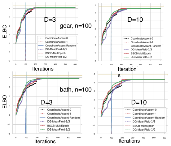
Figure 2: Typical trajectories of multi-epoch algorithms on ELBO objective for Amazon data. 1st row: “gear”; 2nd row: “bath”. Cyan vertical line shows the one-epoch point. Yellow line shows the true log-partition.

Figure 2 records typical trajectories of multi-epoch algorithms for ELBO objectives. Note that the cyan vertical lines indicate the one-epoch point. It shows that after one epoch, DG-MeanField-$1/2$ almost always returns the best solution, and it is also the fastest one to converge. However, CoordinateAscent is quite sensitive to initializations. After sufficiently many iterations, all multi-epoch algorithms converge to similar ELBO values. This is consistent with the intuition because after one epoch, all algorithms are conducting coordinate-wise maximization. One can also observe that the obtained ELBO is close to the true log partition functions (yellow lines).

F.2 Experiments on Shrunken Frank-Wolfe

Though shrunken FW method is not only computationally too expensive, but also have worse approximation guarantee, we still would like to see whether it would produces good solution with more computational resources. In order to verify this, we run all multi-epoch algorithms for 6 epochs, while run shrunken FW for 60 epochs, results are shown in the figure bellow: even with 10 times more computations, shrunken FW still performs worse than the proposed algorithm DG-MeanField-1/2. Sometimes shrunken FW has comparable performance with coordinate descent variant.

F.3 Synthetic Results

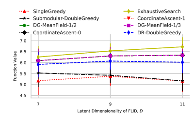
(a) $n=10$

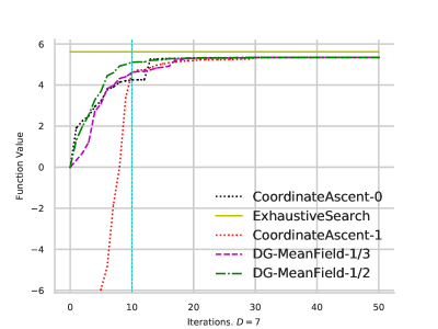
(b) $D=7$

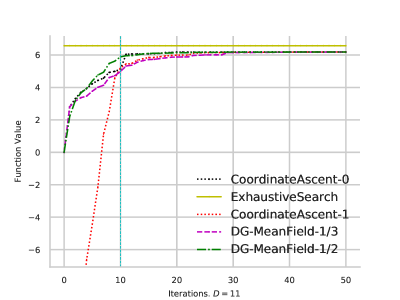
(c) $D=11$

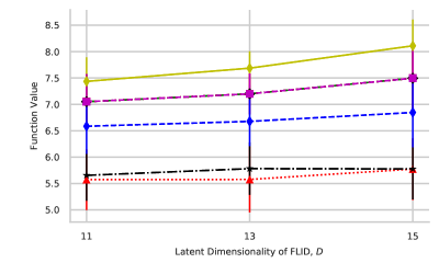
(d) $n=14$

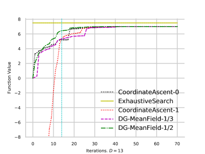
(e) $D=13$

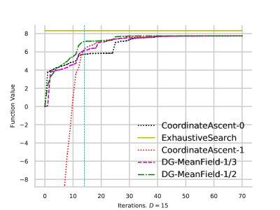
(f) $D=15$

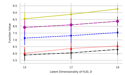
(g) $n=18$

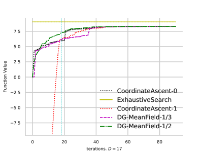
(h) $D=17$

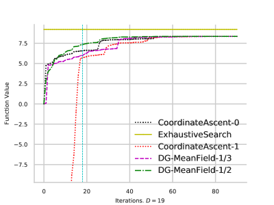
(i) $D=19$

Figure 3: FLID synthetic results. First column shows the function values returned by different algorithms. The other columns show trajectories of multi-epoch algorithms. Cyan vertical line shows one-epoch. Yellow line indicates the true log-partition.

We generate FLID models in the following manner: We firstly generate the latent representation matrix $\mathbf{W}\in{\mathbb{R}}^{n\times D}$ such that each entry of $W_{i,d}\sim U(0,1)$. It is clear that for FLID, $F(\emptyset)=0$. We then set $\mathbf{u}$ to be proportional to $D$ in a random way $\mathbf{u}=0.1D*\mathbf{1}*U(0,1)$ so the objective is non-monotone. Figure 3 records the results: one row corresponds to the results for a specific $n$. First column is the function value returned by the algorithms, which are the average of 10 repeated experiments. The other columns are trajectories of multi-epoch algorithms, since behavior is similar for different repeated experiments, we plot the first one here. Yellow lines are the true log-partition returned by exhaustive search, cyan vertical lines shows the one-epoch point. One can see that for one-epoch algorithms, DR-DoubleGreedy returns the highest value. For multi-epoch algorithms, DG-MeanField-$1/2$ is the fasted one to converge. After sufficiently many epoches, the three multi-epoch algorithms converge to solutions with similar function value.

F.4 More Results on ELBO Objective

See Figure 4 for more results on the ELBO objective from Amazon data.

(a) Legend for subfigs (b,d,g)

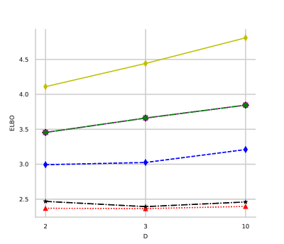
(b) “strollers”, $n=40$

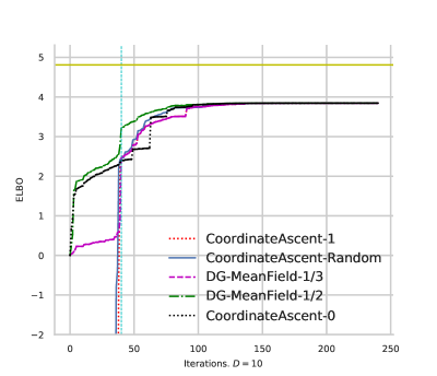
(c) $D=10$

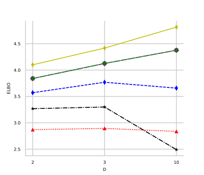
(d) “health”, $n=62$

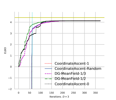
(e) $D=3$

(f) $D=10$

(g) “bath”, $n=100$

(h) $D=3$

(i) $D=10$

Figure 4: ELBO objective on Amazon data. 1st row: “strollers”; 2nd row: “health”. 3rd row: “bath”; Subfigs (b,d,g) shows the ELBO returned by all algorithms, other columns traces trajectories of multi-epoch algorithms. Cyan vertical line show the one-epoch point. Yellow line shows the true log-partition.

F.5 More Results on PA-ELBO Objective

Figure 5 illustrates more results on the PA-ELBO objective from Amazon data.

(a) Legend for subfigs (b,d,g)

(b) “furniture”, $n=40$, folds (6,10)

(c) $D=10$

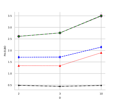
(d) “toys”, $n=62$, folds (6,8)

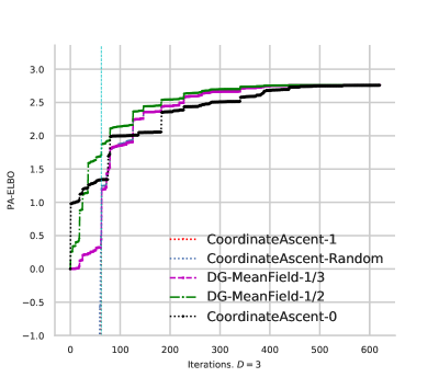
(e) $D=3$

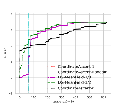
(f) $D=10$

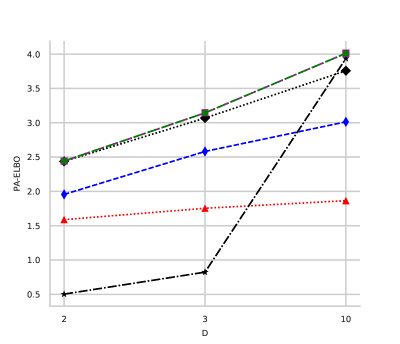
(g) “bedding”, $n=100$, folds (7,9)

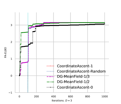
(h) $D=3$

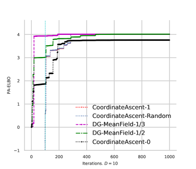
(i) $D=10$

Figure 5: PA-ELBO objective on Amazon data. First row: “furniture”; second row: “toys”; third row: “bedding”. Subfigs (b,d,g) show the PA-ELBO returned by all algorithms, other columns traces trajectories of multi-epoch algorithms. Cyan vertical line shows the one-epoch point.

References

- Bach [2015] Bach, Francis. Submodular functions: from discrete to continuous domains. arXiv preprint arXiv:1511.00394, 2015.
- Bian et al. [2017a] Bian, A. An, Buhmann, Joachim M., Krause, Andreas, and Tschiatschek, Sebastian. Guarantees for greedy maximization of non-submodular functions with applications. In International Conference on Machine Learning (ICML), 2017a.
- Bian et al. [2017b] Bian, A. An, Mirzasoleiman, Baharan, Buhmann, Joachim M., and Krause, Andreas. Guaranteed non-convex optimization: Submodular maximization over continuous domains. In International Conference on Artificial Intelligence and Statistics (AISTATS), pp. 111–120, 2017b.
- Bian et al. [2017c] Bian, An, Levy, Kfir Y., Krause, Andreas, and Buhmann, Joachim M. Continuous dr-submodular maximization: Structure and algorithms. In Advances in Neural Information Processing Systems (NIPS), pp. 486–496, 2017c.
- Bian et al. [2016] Bian, Yatao, Gronskiy, Alexey, and Buhmann, Joachim M. Information-theoretic analysis of maxcut algorithms. In IEEE Information Theory and Applications Workshop (ITA), pp. 1–5, 2016. URL http://people.inf.ethz.ch/ybian/docs/pa.pdf.
- Buchbinder et al. [2012] Buchbinder, Niv, Feldman, Moran, Naor, Joseph, and Schwartz, Roy. A tight linear time (1/2)-approximation for unconstrained submodular maximization. In Foundations of Computer Science (FOCS), 2012 IEEE 53rd Annual Symposium on, pp. 649–658. IEEE, 2012.
- Buhmann [2010] Buhmann, Joachim M. Information theoretic model validation for clustering. In Information Theory Proceedings (ISIT), 2010 IEEE International Symposium on, pp. 1398–1402. IEEE, 2010.
- Buhmann et al. [2018] Buhmann, Joachim M, Dumazert, Julien, Gronskiy, Alexey, and Szpankowski, Wojciech. Posterior agreement for large parameter-rich optimization problems. to appear in TCS, 2018. URL https://www.cs.purdue.edu/homes/spa/papers/tcs-sub.pdf.
- Clinescu et al. [2007] Clinescu, Gruia, Chekuri, Chandra, Pál, Martin, and Vondrák, Jan. Maximizing a submodular set function subject to a matroid constraint. In Integer programming and combinatorial optimization, pp. 182–196. Springer, 2007.
- Calinescu et al. [2007] Calinescu, Gruia, Chekuri, Chandra, Pál, Martin, and Vondrák, Jan. Maximizing a submodular set function subject to a matroid constraint (extended abstract). In IPCO, pp. 182–196, 2007.
- Chekuri et al. [2014] Chekuri, Chandra, Vondrák, Jan, and Zenklusen, Rico. Submodular function maximization via the multilinear relaxation and contention resolution schemes. SIAM Journal on Computing, 43(6):1831–1879, 2014.
- Chekuri et al. [2015] Chekuri, Chandra, Jayram, TS, and Vondrák, Jan. On multiplicative weight updates for concave and submodular function maximization. In Proceedings of the 2015 Conference on Innovations in Theoretical Computer Science, pp. 201–210. ACM, 2015.
- Chen et al. [2018] Chen, Lin, Hassani, Hamed, and Karbasi, Amin. Online continuous submodular maximization. In International Conference on Artificial Intelligence and Statistics (AISTATS), pp. 1896–1905, 2018.
- Djolonga & Krause [2014] Djolonga, Josip and Krause, Andreas. From map to marginals: Variational inference in bayesian submodular models. In Neural Information Processing Systems (NIPS), 2014.
- Djolonga & Krause [2015] Djolonga, Josip and Krause, Andreas. Scalable variational inference in log-supermodular models. In International Conference on Machine Learning (ICML), 2015.
- Djolonga et al. [2016] Djolonga, Josip, Tschiatschek, Sebastian, and Krause, Andreas. Variational inference in mixed probabilistic submodular models. In Advances in Neural Information Processing Systems (NIPS), pp. 1759–1767, 2016.
- Ene & Nguyen [2016] Ene, Alina and Nguyen, Huy L. A reduction for optimizing lattice submodular functions with diminishing returns. arXiv preprint arXiv:1606.08362, 2016.
- Feige et al. [2011] Feige, Uriel, Mirrokni, Vahab S, and Vondrak, Jan. Maximizing non-monotone submodular functions. SIAM Journal on Computing, 40(4):1133–1153, 2011.
- Gillenwater et al. [2012] Gillenwater, Jennifer, Kulesza, Alex, and Taskar, Ben. Near-optimal map inference for determinantal point processes. In Advances in Neural Information Processing Systems, pp. 2735–2743, 2012.
- Gillenwater et al. [2014] Gillenwater, Jennifer A, Kulesza, Alex, Fox, Emily, and Taskar, Ben. Expectation-maximization for learning determinantal point processes. In Advances in Neural Information Processing Systems (NIPS), pp. 3149–3157, 2014.
- Gorbach et al. [2017] Gorbach, Nico S, Bian, A. An, Fischer, Benjamin, Bauer, Stefan, and Buhmann, Joachim M. Model selection for Gaussian process regression. In German Conference on Pattern Recognition, pp. 306–318, 2017.
- Gottschalk & Peis [2015] Gottschalk, Corinna and Peis, Britta. Submodular function maximization on the bounded integer lattice. In Approximation and Online Algorithms, pp. 133–144. Springer, 2015.
- Gronskiy & Buhmann [2014] Gronskiy, Alexey and Buhmann, Joachim M. How informative are minimum spanning tree algorithms? In Information Theory (ISIT), 2014 IEEE International Symposium on, pp. 2277–2281. IEEE, 2014.
- Hoeffding [1963] Hoeffding, Wassily. Probability inequalities for sums of bounded random variables. Journal of the American statistical association, 58(301):13–30, 1963.
- Iyer & Bilmes [2015] Iyer, Rishabh and Bilmes, Jeffrey. Submodular point processes with applications to machine learning. In Artificial Intelligence and Statistics, pp. 388–397, 2015.
- Krause & Cevher [2010] Krause, Andreas and Cevher, Volkan. Submodular dictionary selection for sparse representation. In Proceedings of the 27th International Conference on Machine Learning (ICML), pp. 567–574, 2010.
- Krause & Golovin [2012] Krause, Andreas and Golovin, Daniel. Submodular function maximization. Tractability: Practical Approaches to Hard Problems, 3:19, 2012.
- Krause & Guestrin [2005] Krause, Andreas and Guestrin, Carlos. Near-optimal nonmyopic value of information in graphical models. In 21st conference on uncertainty in artificial intelligence (UAI), 2005.
- Kulesza et al. [2012] Kulesza, Alex, Taskar, Ben, et al. Determinantal point processes for machine learning. Foundations and Trends® in Machine Learning, 5(2–3):123–286, 2012.
- Lin & Bilmes [2011a] Lin, Hui and Bilmes, Jeff. A class of submodular functions for document summarization. In Proceedings of the 49th Annual Meeting of the Association for Computational Linguistics: Human Language Technologies-Volume 1, pp. 510–520. Association for Computational Linguistics, 2011a.
- Lin & Bilmes [2011b] Lin, Hui and Bilmes, Jeff. Optimal selection of limited vocabulary speech corpora. In Twelfth Annual Conference of the International Speech Communication Association, 2011b.
- Lovász [1983] Lovász, László. Submodular functions and convexity. In Mathematical Programming The State of the Art, pp. 235–257. Springer, 1983.
- Mokhtari et al. [2018] Mokhtari, Aryan, Hassani, Hamed, and Karbasi, Amin. Decentralized submodular maximization: Bridging discrete and continuous settings. arXiv preprint arXiv:1802.03825, 2018.
- Niazadeh et al. [2018] Niazadeh, Rad, Roughgarden, Tim, and Wang, Joshua R. Optimal algorithms for continuous non-monotone submodular and dr-submodular maximization. arXiv preprint arXiv:1805.09480, 2018.
- Soma & Yoshida [2017] Soma, Tasuku and Yoshida, Yuichi. Non-monotone dr-submodular function maximization. In AAAI, volume 17, pp. 898–904, 2017.
- Staib & Jegelka [2017] Staib, Matthew and Jegelka, Stefanie. Robust budget allocation via continuous submodular functions. In Proceedings of the 34th International Conference on Machine Learning (ICML), 2017.
- Tschiatschek et al. [2016] Tschiatschek, Sebastian, Djolonga, Josip, and Krause, Andreas. Learning probabilistic submodular diversity models via noise contrastive estimation. In Proc. International Conference on Artificial Intelligence and Statistics (AISTATS), 2016.
- Vondrák [2008] Vondrák, Jan. Optimal approximation for the submodular welfare problem in the value oracle model. In Proceedings of the 40th Annual ACM Symposium on Theory of Computing, pp. 67–74, 2008.
- Wainwright et al. [2008] Wainwright, Martin J, Jordan, Michael I, et al. Graphical models, exponential families, and variational inference. Foundations and Trends® in Machine Learning, 1(1–2):1–305, 2008.
- Wilder [2017] Wilder, Bryan. Risk-sensitive submodular optimization. In AAAI, 2017.
- Zheng et al. [2015] Zheng, Shuai, Jayasumana, Sadeep, Romera-Paredes, Bernardino, Vineet, Vibhav, Su, Zhizhong, Du, Dalong, Huang, Chang, and Torr, Philip HS. Conditional random fields as recurrent neural networks. In Proceedings of the IEEE International Conference on Computer Vision, pp. 1529–1537, 2015.