Projection-Free Bandit Convex Optimization

Abstract

In this paper, we propose the first computationally efficient projection-free algorithm for bandit convex optimization (BCO). We show that our algorithm achieves a sublinear regret of $O(nT^{4/5})$ (where $T$ is the horizon and $n$ is the dimension) for any bounded convex functions with uniformly bounded gradients. We also evaluate the performance of our algorithm against baselines on both synthetic and real data sets for quadratic programming, portfolio selection and matrix completion problems.

1 Introduction

The online learning setting models a dynamic optimization process in which data becomes available in a sequential manner and the learning algorithm has to adjust and update its predictor as more data is disclosed. It can be best formulated as a repeated two-player game between a learner and an adversary as follows. At each iteration $t$, the learner commits to a decision $\Bx_{t}$ from a constraint set $\mathcal{K}\subseteq\mathbb{R}^{n}$. Then, the adversary selects a cost function $f_{t}$ and the learner suffers the loss $f_{t}(\Bx_{t})$ in addition to receiving feedback. In the online learning model, it is generally assumed that the learner has access to a gradient oracle for all loss functions $f_{t}$, and thus knows the loss had she chosen a different point at iteration $t$. The performance of an online learning algorithm is measured by a game theoretic metric known as regret which is defined as the gap between the total loss that the learner has incurred after $T$ iterations and that of the best fixed decision in hindsight.

In online learning, we are usually interested in sublinear regret as a function of the horizon $T$. To this end, other structural assumptions are made. For instance, when all the loss functions $f_{t}$, as well as the constraint set $\mathcal{K}$, are convex, the problem is known as Online Convex Optimization (OCO) (Zinkevich, 2003). This framework has received a lot of attention due to its capability to model diverse problems in machine learning and statistics such as spam filtering, ad selection for search engines, and recommender systems, to name a few. It is known that the online projected gradient descent algorithm achieves a tight $O(\sqrt{T})$ regret bound (Zinkevich, 2003). However, in many modern machine learning scenarios, one of the main computational bottlenecks is the projection onto the constraint set $\mathcal{K}$. For example, in recommender systems and matrix completion, projections amount to expensive linear algebraic operations. Similarly, projections onto matroid polytopes with exponentially many linear inequalities are daunting tasks in general. This difficulty has motivated the use of projection-free algorithms  (Hazan and Kale, 2012; Hazan, 2016; Chen et al., 2018) for which the most efficient one achieves $O(T^{3/4})$ regret.

In this paper, we consider a more difficult, and very often more realistic, OCO setting where the feedback is incomplete. More precisely, we consider a bandit feedback model where the only information observed by the learner at iteration $t$ is the loss $f_{t}(\Bx_{t})$ at the point $\Bx_{t}$ that she has chosen. In particular, the learner does not know the loss had she chosen a different point $\Bx_{t}$. Therefore, the learner has to balance between exploiting the information that she has gathered and exploring the new data. This exploration-exploitation balance has been done beautifully by (Flaxman et al., 2005) to achieve $O(T^{3/4})$ regret. With extra assumption on the loss functions (e.g., strong convexity), the regret bound has been recently improved to $\tilde{O}(T^{1/2})$  (Hazan and Li, 2016; Bubeck et al., 2015, 2017). Again, all these works either rely on the computationally expensive projection operations or inverting the Hessian matrix of a self-concordant barrier. In addition, regret bounds usually have a very high polynomial dependency on the dimension.

In this paper, we develop the first computationally efficient projection-free algorithm with a sublinear regret bound of $O(T^{4/5})$ on the expected regret. We also show that the dependency on the dimension is linear. The regret bounds in different OCO settings are summarized in Table 1.

[t] Online Bandit Projection $O(T^{1/2})$^$\dagger$ $O(T^{3/4})$^$\ddagger$, $\tilde{O}(T^{1/2})$^$\sharp$ Projection-free $O(T^{3/4})$^$\flat$ $O(T^{4/5})$ (this work)

• Zinkevich (2003)

• Flaxman et al. (2005)

• Hazan and Li (2016); Bubeck et al. (2015, 2017)

• Hazan and Kale (2012)(Hazan, 2016, Alg. 24)

Table 1: Regret bounds in various settings of adversarial online convex optimization.

Our Contributions

Sublinear regret with computational efficiency. While there is a line of recent work that attains the minimax bound (Hazan and Li, 2016; Bubeck et al., 2015, 2017), these algorithms have computationally expensive parts, such as inverting the Hessian of the self-concordant barrier. In contrast to these works that seek the lowest regret bound, we try to find a computationally efficient solution that attains a sublinear regret bound. Therefore, we have to avoid computationally expensive techniques like projection, Dikin ellipsoid and self-concordant barrier. As is shown in the experiments, our algorithm is simple and effective as it only requires solving a linear optimization problem, while preserving a sublinear regret bound.

Techniques. The Frank-Wolfe (FW) algorithm may perform arbitrarily poorly with stochastic gradients even in the offline setting (Hassani et al., 2017). Since the one-point estimator of gradient has a large variance, a simple combination of online FW (Hazan and Kale, 2012) and one-point estimator (Flaxman et al., 2005) may not work. This is in fact shown empirically in Fig 1(a) when the loss functions are quadratic. In addition, the online FW algorithm of Hazan and Kale (2012) is infeasible in the bandit setting. Basically, in each iteration of the online FW, the linear objective is the average gradient of all previous functions at a new point $x_{t}$. Note that in the bandit setting, it is impossible to evaluate the gradient of $f_{i}$ at $x_{t}$ ($i<t$), even with one-point estimators of Flaxman et al. (2005).

Our work has two major differences with (Hazan and Kale, 2012). First, to make it a bandit algorithm, our linear objective is the sum of previously estimated gradients ($\sum_{\tau=1}^{t-1}\Bg_{\tau}$, where $\Bg_{\tau}$ is the one-point estimator of $\nabla f_{\tau}(\Bx_{\tau})$), rather than $\sum_{\tau=1}^{t-1}\nabla f_{\tau}(\Bx_{t-1})$. Second, we add a regularizer to stabilize the prediction.

2 Preliminaries

Notation

We let $S^{n}\triangleq\{\Bx\in\mathbb{R}^{n}:\|\Bx\|=1\}$ and $B^{n}\triangleq\{\Bx\in\mathbb{R}^{n}:\|\Bx\|\leq 1\}$ denote the unit sphere and the unit ball in the $n$-dimensional Euclidean space, respectively. Let $\Bv$ be a random vector. We write $\Bv\sim S^{n}$ and $\Bv\sim B^{n}$ to indicate that $\Bv$ is uniformly distributed over $S^{n}$ and $B^{n}$, respectively.

For any point set $\CD\subseteq\mathbb{R}^{n}$ and $\alpha>0$, we denote $\{\Bx\in\mathbb{R}^{n}:\frac{1}{\alpha}\Bx\in\CD\}$ by $\alpha\CD$. Let $f:\CD\to\mathbb{R}$ be a real-valued function on domain $\CD\subseteq\mathbb{R}^{n}$. Its sup norm is given by $\|f\|_{\infty}\triangleq\sup_{\Bx\in\CD}|f(\Bx)|$. We say that the function $f:\CD\to\mathbb{R}$ is $\alpha$-strongly convex (Nesterov, 2003, pp. 63–64) if $f$ is continuously differentiable, $\CD$ is a convex set, and the following inequality holds for $\forall\Bx,\By\in\CD$

$$f(\By)\geq(\Bx)+\nabla f(\Bx)^{\top}(\By-\Bx)+\frac{1}{2}\alpha\|\By-\Bx\|^{2}.$$

An equivalent definition of strong convexity is $(\nabla f(\Bx)-\nabla f(\By))^{\top}(\Bx-\By)\geq\alpha\|\Bx-\By\|^{2},$ for all $\Bx,\By\in\CD$. We say that $f$ is $G$-Lipschitz if $\forall\Bx,\By\in\CD$, $\|f(\Bx)-f(\By)\|\leq G\|\Bx-\By\|$. In this paper, we assume that the loss functions are all convex and bounded, meaning that there is a finite $M$ such that $\|f\|_{\infty}\leq M$. We also assume that they are differentiable with uniformly bounded gradients, i.e., there exists a finite $G$ such that $\|\nabla f\|_{\infty}\leq G$.

Bandit Convex Optimization

Online convex optimization is performed in a sequence of consecutive rounds, where at round $t$, a learner has to choose an action $\Bx_{t}$ from a convex decision set $\mathcal{K}\subseteq\mathbb{R}^{n}$. Then, an adversary chooses a loss function $f_{t}$ from a family $\CF$ of bounded convex functions. Once the action and the loss function are determined, the learner suffers a loss $f_{t}(\Bx_{t})$. The aim is to minimize regret which is the gap between the accumulated loss and the minimum loss in hindsight. More formally, the regret of a learning algorithm $\CA$ after $T$ rounds is given by

$$\CR_{\CA,T}\triangleq\sup_{\{f_{1},\dots,f_{T}\}\subseteq\CF}\left\{\sum_{t=1}^{T}f_{t}(\Bx_{t})-\min_{\Bx\in\CD}\sum_{t=1}^{T}f_{t}(\Bx)\right\}.$$

In the full information setting, the learner receives the loss function $f_{t}$ as a feedback (usually by having access to the gradient of $f_{t}$ at any feasible decision domain). In the bandit setting, however, the feedback is limited to the loss at the point that she has chosen, i.e., $f_{t}(\Bx_{t})$. In this paper, we consider the bandit setting where the family $\CF$ consists of bounded convex functions with uniformly bounded gradients. Under these conditions, we propose a projection-free algorithm $\CA$ that achieves an expected regret of $\operatorname{\mathbb{E}}[\CR_{\CA,T}]=O(T^{4/5})$.

Smoothing

A key ingredient of our solution relies on constructing the smoothed version of loss functions. Formally, for a function $f$, its $\delta$-smoothed version is defined by

$$\hat{f}_{\delta}(\Bx)=\operatorname{\mathbb{E}}_{\Bv\sim B^{n}}[f(\Bx+\delta\Bv)],$$

where $\Bv$ is drawn uniformly at random from the $n$-dimensional unit ball $B^{n}$. Here, $\delta$ controls the radius of the ball that the function $f$ is averaged over. Since $\hat{f}_{\delta}$ is a smoothed version of $f$, it inherits analytical properties from $f$. Lemma 1 formalizes this idea.

Lemma 1 (Lemma 2.6 in (Hazan, 2016)).

Let $f:\CD\subseteq\mathbb{R}^{n}\to\mathbb{R}$ be a convex, $G$-Lipschitz continuous function and let $\CD_{0}\subseteq\CD$ be such that $\forall\Bx\in\CD_{0},\Bv\in S^{n}$, $\Bx+\delta\Bv\in\CD$. Let $\hat{f}_{\delta}$ be the $\delta$-smoothed function defined above. Then $\hat{f}_{\delta}$ is also convex, and $\|\hat{f}_{\delta}-f\|_{\infty}\leq\delta G$ on $\CD_{0}$.

Since $\hat{f}_{\delta}$ is an approximation of $f$, if one finds a minimizer of $\hat{f}_{\delta}$, Lemma 1 implies that it also minimizes $f$ approximately. Another advantage of considering the smoothed version is that it admits one-point gradient estimates of $\hat{f}_{\delta}$ based on samples of $f$. This idea was first introduced in (Flaxman et al., 2005) for developing an online gradient descent algorithm without having access to gradients.

Lemma 2 (Lemma 6.4 in (Hazan, 2016)).

Let $\delta>0$ be any fixed positive real number and $\hat{f}_{\delta}$ be the $\delta$-smoothed version of function $f$. The following equation holds

$$\nabla\hat{f}_{\delta}(\Bx)=\operatorname{\mathbb{E}}_{\Bu\sim S^{n}}\left[\frac{n}{\delta}f(\Bx+\delta\Bu)\Bu\right].$$ (1)

Lemma 2 suggests that in order to sample the gradient of $\hat{f}_{\delta}$ at a point $\Bx$, it suffices to evaluate $f$ at a random point $\Bx+\delta\Bu$ around the point $\Bx$.

3 Algorithms and Main Results

The first key idea of our proposed algorithm is to construct a follow-the-regularized-leader objective

$$F_{t}(\Bx)=\eta\sum_{\tau=1}^{t-1}\nabla f_{\tau}(\Bx_{\tau})^{\top}\Bx+\|\Bx-\Bx_{1}\|^{2}.$$ (2)

Instead of minimizing $F_{t}$ directly (as it is done in follow-the-regularized-leader algorithm), the learner first solves a linear program over the decision set $\mathcal{K}$

$$\Bv_{t}=\min_{\Bx\in\mathcal{K}}\{\nabla F_{t}(\Bx_{t})\cdot\Bx\},$$ (3)

and then updates its decision as follows

$$\Bx_{t+1}\leftarrow(1-\sigma_{t})\Bx_{t}+\sigma_{t}\Bv_{t}.$$ (4)

Note that minimizing $F_{t}$ requires solving a quadratic optimization problem, which is as computationally prohibitive as a projection operation. In contrast, since the update in Eq. 4 is a convex combination between $\Bv_{t}$ and $\Bx_{t}$, the iterates always lie inside the convex decision set $\mathcal{K}$, thus no projection is needed. This is the main idea behind the online conditional gradient algorithm (Algorithm 24 in (Hazan, 2016)). In the bandit setting (the focus of this paper), the gradients $\nabla f_{\tau}(\Bx_{\tau})$ are unavailable, hence the learner cannot perform steps (2) and (3). To tackle this issue, we introduce the second ingredient of our algorithm, namely, the smoothing and one-point gradient estimates (Flaxman et al., 2005). Formally, at the $t$-th iteration, rather than selecting $\Bx_{t}$, the learner plays a random point $\By_{t}$ that is $\delta$-close to $\Bx_{t}$ and in return observes the cost $f_{t}(\By_{t})$. As shown in Lemma 2, $f_{t}(\By_{t})$ can be used to construct an unbiased estimate $\Bg_{t}$ for the gradient of the $\delta$-smoothed version of $f_{t}$ at point $\Bx_{t}$, i.e., $\operatorname{\mathbb{E}}[\Bg_{t}]=\nabla\hat{f}_{t,\delta}(\Bx_{t})$, where $\hat{f}_{t,\delta}(\Bx_{t})\triangleq\operatorname{\mathbb{E}}_{\Bv\sim B^{n}}[f_{t}(\Bx_{t}+\delta\Bv)]$. This observation suggests that we can replace $\nabla f_{t}(\Bx_{t})$ by $\Bg_{t}$ in the follow-the-regularized-leader objective (2) to obtain a variant that relies on the one-point gradient estimate, i.e.,

$$F_{t}(\Bx)=\eta\sum_{\tau=1}^{t-1}\Bg_{\tau}^{\top}\Bx+\|\Bx-\Bx_{1}\|^{2}.$$ (5)

Note that forming $F_{t}(\Bx)$ in (5) is fully realizable for a learner in a bandit setting. The full description of our algorithm is outlined in Algorithm 1. Even though the objective function $F_{t}(\Bx)$ relies on the unbiased estimates of the smoothed versions of $f_{t}$ (rather than $f_{t}$ itself), it is not far off from the original objective (shown in Eq. 2) if the distance between the random point $\By_{t}$ and the point $\Bx_{t}$ is properly chosen. Therefore, minimizing the sum of smoothed versions of $f_{t}$ (as it is done by Algorithm 1) will end up minimizing the actual regret. This intuition is formally proven in Theorem 1. Without loss of generality, we assume additionally that the constraint $\mathcal{K}$ contains a ball of radius $r$ centered at the origin (this is always achievable by shrinking the constraint set as long as it has a non-empty interior).

1:horizon $T$, constraint set $\mathcal{K}$

2:$\By_{1},\By_{2},\dots,\By_{T}$

3:$\Bx_{1}\in(1-\alpha)\mathcal{K}$

4:for $t=1,\ldots,T$ do

5:     $\By_{t}\leftarrow\Bx_{t}+\delta\Bu_{t}$, where $\Bu_{t}\sim S^{n}$

6:     Play $\By_{t}$ and observe $f_{t}(\By_{t})$

7:     $\Bg_{t}\leftarrow\frac{n}{\delta}f_{t}(\By_{t})\Bu_{t}$ $\triangleright$ $\Bg_{t}$ is an unbiased estimator of $\nabla\hat{f}_{t,\delta}(\Bx_{t})$

8:     $F_{t}(\Bx)\leftarrow\eta\sum_{\tau=1}^{t-1}\Bg_{\tau}^{\top}\Bx+\|\Bx-\Bx_{1}\|^{2}$

9:     $\Bv_{t}\leftarrow\operatorname*{arg\,min}_{\Bx\in(1-\alpha)\mathcal{K}}\{\nabla F_{t}(\Bx_{t})\cdot\Bx\}$$\triangleright$ Solve a linear optimization problem

10:     $\Bx_{t+1}\leftarrow(1-\sigma_{t})\Bx_{t}+\sigma_{t}\Bv_{t}$

11:end for

Algorithm 1 Projection-Free Bandit Convex Optimization

Theorem 1 (Proof in Section 5).

Assume that for every $t\in\mathbb{N}_{\geq 1}$, $f_{t}$ is convex, $\|f_{t}\|_{\infty}\leq M$ on $\mathcal{K}$, $\sup_{\Bx\in\mathcal{K}}\|\nabla f_{t}(\Bx)\|\leq G$, $rB^{n}\subseteq\mathcal{K}\subseteq RB^{n}$, and that the diameter of $\mathcal{K}$ is $D<\infty$. If we set $\eta=\frac{D}{\sqrt{2}nM}T^{-4/5}$, $\sigma_{t}=t^{-2/5}$, $\delta=cT^{-1/5}$, and $\alpha=\delta/r<1$ in Algorithm 1, where $c>0$ is a constant, we have $\By_{t}\in\mathcal{K},\forall 1\leq t\leq T$. Moreover, the expected regret $\operatorname{\mathbb{E}}[\CR_{\CA,T}]$ up to horizon $T$ is at most

$$\frac{\sqrt{2}nMD}{c^{2}}T^{3/5}+(\sqrt{2}nMD+\frac{5\sqrt{2}}{4}DG+3cG+cRG/r)T^{4/5}.\\$$

Note that the regret bound of Algorithm 1 depends linearly on the dimension $n$.

A minor drawback of Algorithm 1 is that it requires the knowledge of the horizon $T$. This problem can be easily circumvented via the doubling trick while preserving the regret bound of Theorem 1. The doubling trick was first proposed in (Auer et al., 1995) and its key idea is to invoke the base algorithm repeatedly with a doubling horizon. Algorithm 2 outlines an anytime algorithm for BCO using the doubling trick. Theorem 2 shows that for any $t\geq 1$, the expected regret of Algorithm 2 by the end of the $t$-th iteration is bounded by $O(t^{4/5})$.

1:constraint set $\mathcal{K}$

2:$\By_{1},\By_{2},\dots$

3:for $m=0,1,2,\ldots$ do

4:     Run Algorithm 1 with horizon $2^{m}$ from the $2^{m}$-th iteration (inclusive) to the $(2^{m+1}-1)$-th iteration (inclusive).

5:     Let $\By_{2^{m}},\dots,\By_{2^{m+1}-1}$ be the points that Algorithm 1 selects for the objectives $f_{2^{m}},\dots,f_{2^{m+1}-1}$.

6:end for

Algorithm 2 Anytime Projection-Free Bandit Convex Optimization

Theorem 2 (Proof in Appendix B).

If the regret bound of Algorithm 1 for horizon $T$ is $\beta T^{4/5}$, then for any $t\geq 1$, the expected regret of Algorithm 2 by the end of the $t$-th iteration is at most

$$\operatorname{\mathbb{E}}[\CR_{\CA,T}]=\frac{\beta}{1-2^{-4/5}}(t+1)^{4/5}=O(t^{4/5}).$$

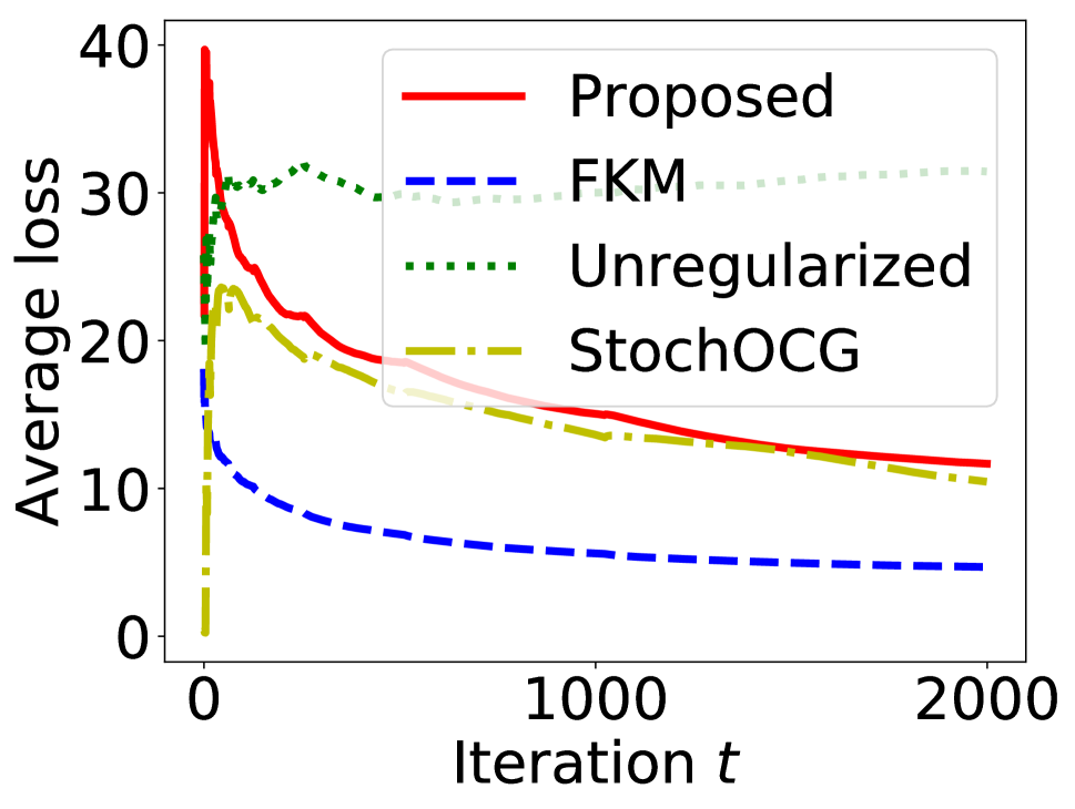
(a) Quadratic programming

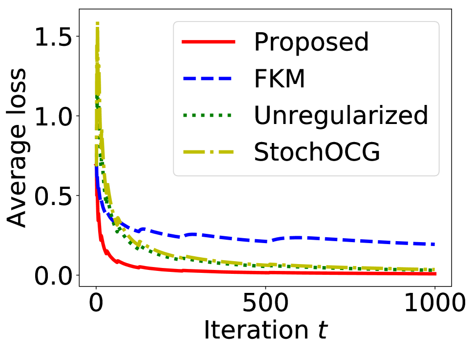
(b) Portfolio selection

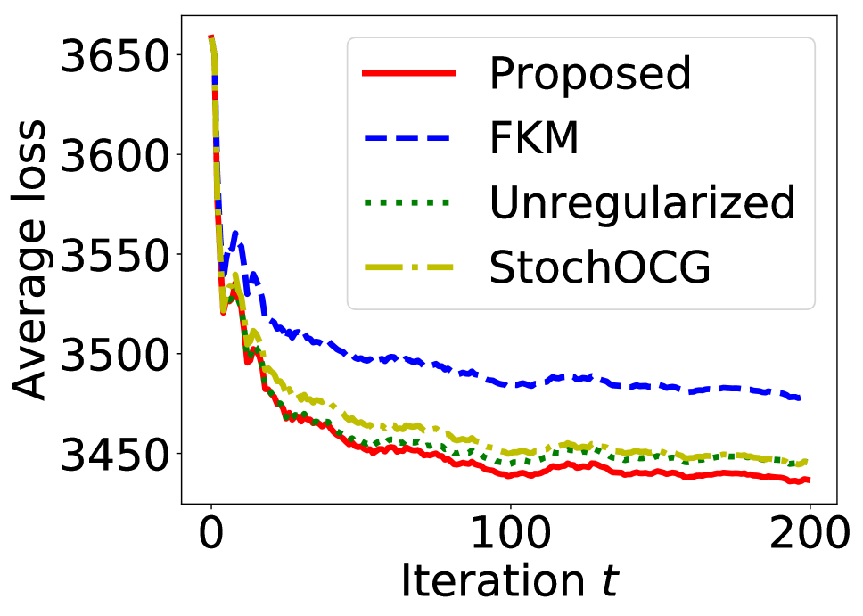
(c) Matrix completion

(d) Relative execution time

Figure 1: In Figs. 1(a), 1(b) and 1(c), we show the average loss versus the number of iterations in the three sets of experiments. The relative execution time is shown in Fig. 1(d), where the execution time of the proposed algorithm is set to $1$.

4 Experiments

In our set of experiments, we compare Algorithm 2 with the following baselines:

• FKM: Online projected gradient descent with spherical gradient estimators (Flaxman et al., 2005).

• Unregularized: A variant of our proposed algorithm without the regularizer $\|\Bx-\Bx_{1}\|^{2}$ in line 8 of Algorithm 1.

• StochOCG: Online conditional gradient (Hazan, 2016) with stochastic gradients (not a bandit algorithm). Such stochastic gradients are formed by adding Gaussian noise with standard deviation $n$ to the exact gradients.

The anytime version of the algorithms (obtained via the doubling trick) is used. Therefore the horizon $T$ is unknown to the algorithms. Note that the standard deviation of the point estimate used in FKM and our proposed method is proportional to the dimension $n$. This is why the standard deviation of the Gaussian noise in StochOCG is set to $n$ to make the noise in the gradients comparable.

We performed three sets of experiments in total. In all of them we report the average loss defined as $\operatorname{\mathbb{E}}[\sum_{t=1}^{T}f_{t}(\Bx_{t})]/T$.

Quadratic programming: In the first experiment, the loss functions are quadratic, i.e., $f_{t}(\Bx)=\frac{1}{2}\Bx^{\top}\BG_{t}^{\top}\BG_{t}\Bx+\Bw_{t}^{\top}\Bx$. Each entry of $\BG_{t}$ and $\Bw_{t}$ is sampled from the standard normal distribution. The convex constraint of this problem is a polytope $\{\Bx:\bm{0}\leq\Bx\leq\bm{1},\BA\Bx\leq\bm{1}\}$ and each entry of $\BA$ is sampled from the uniform distribution on $[0,1]$. The average loss is illustrated in Fig. 1(a). We observe that the average loss of our proposed algorithm declines as the number of iterations increases. This agrees with the theoretical sublinear regret bound. StochOCG has a similar performance while FKM exhibits the lowest loss. In contrast, the loss of Unregularized appears to be linear which shows the significance of regularization to achieve low regret. This observation also suggests that simply combining (Hazan and Kale, 2012) and smoothing may not work in practice.

Portfolio selection: For this experiment, we randomly select $n=100$ stocks from Standard & Poor’s 500 index component stocks and consider their prices during the business days between February 18th, 2013 and November 27th, 2017. We follow the formulation in (Hazan, 2016, Section 1.2). Let $\Br_{t}\in\mathbb{R}^{n}$ be a vector such that $\Br_{t}(i)$ is the ratio of the price of stock $i$ on day $t+1$ to its price on day $t$. An investor is trying maximize her wealth by investing on different stock options. If $W_{t}$ denotes her wealth on day $t$, then we have the following recursion: $W_{t+1}=W_{t}\cdot\Br_{t}^{\top}\Bx_{t}$. After $T$ days of investments, the total wealth will be $W_{T}=W_{1}\cdot\prod_{t=1}^{T}\Br_{t}^{\top}\Bx_{t}$. To maximize the wealth, the investor has to maximize $\sum_{t=1}^{T}\log(\Br_{t}^{\top}\Bx_{t})$, or equivalently minimize its negation. Thus, we can define $f_{t}(\Bx_{t})\triangleq-\log(\Br_{t}^{\top}\Bx_{t})$. FKM requires that the constraint set contains the unit ball. To this end, we set $\By_{t}=2n\Bx_{t}-1$ so that $\By_{t}$ lies in an enlarged region $\Delta^{\prime}_{n}\triangleq\{\By\in\mathbb{R}^{n}:-1\leq\By(i)\leq 2n-1,\sum_{i=1}^{n}\By(i)\leq n\}$. In addition, the objective functions $f_{t}$ are viewed as functions of $\By_{t}$ rather than $\Bx_{t}$. The average losses versus the number of iterations are presented in Fig. 1(b). Our proposed algorithm has the lowest loss in this set of experiments while FKM has the largest.

Matrix completion: Let $\{\BM_{t}\}_{t=1}^{T}$ be symmetric positive semi-definite (PSD) matrices, where $\BM_{t}=\BN_{t}^{\top}\BN_{t}$ and every entry of $\BN_{t}\in\mathbb{R}^{k\times n}$ obeys the standard normal distribution. At each iteration, half of the entries of $\BM_{t}$ are observed. We set $n=20$ and $k=18$. We denote the entries of $\BM_{t}$ disclosed at the $t$-th iteration by $O_{t}$. We want to minimize $f_{t}(\BX_{t})\triangleq\frac{1}{2}\sum_{(i,j)\in O_{t}}(\BX_{t}[i,j]-\BM_{t}[i,j])^{2}$ subject to $\|\BX_{t}\|_{*}\leq k$, where $\BX_{t}$ is of the same shape as $\BM_{t}$ and $\|\cdot\|_{*}$ denotes the nuclear norm. The nuclear norm constraint is a standard convex relaxation of the rank constraint $\operatorname{rank}(\BX)\leq k$. The linear optimization step in 9 of Algorithm 1 has a closed-form solution $\Bv_{t}=k\Bv_{\max}\Bv_{\max}^{\top}$, where $\Bv_{\max}$ is the eigenvector of the largest eigenvalue of $-\nabla f_{t}(\BX_{t})$ (Hazan, 2016, Section 7.3.1). The largest eigenvector can be computed very efficiently using power iterations, whilst it is extremely costly to perform projection onto a convex subset of the space of PSD matrices. As shown in Fig. 1(d), the efficiency of the proposed algorithm is $61$ times that of the projection-based FKM algorithm. The average loss of the algorithms is shown in Fig. 1(c). Our proposed algorithm outperforms the other baselines while FKM suffers the largest loss.

We also observe rises of the curves at their initial stage in Fig. 1. They are due to the doubling trick (Algorithm 2) and a small denominator of the average loss. The unknown horizon is divided into epochs with a doubling size (1, 2, 4, and so forth). When the algorithm starts a new epoch, everything is reset and the algorithm learns from scratch. Furthermore, the denominator of the average loss is small (it is initially 1, and then becomes 2, 3, 4, and so forth) at the initial stage. Therefore, due to the frequent resets and a small denominator, the behavior is less stable. As the epoch size and denominator grow, the average loss declines steadily.

The execution time is shown in Fig. 1(d). It was measured on eight Intel Xeon E5-2660 V2 cores and the algorithms were implemented in Julia. 50 repeated experiments were run in parallel. It can be observed that our proposed algorithm runs significantly faster than the FKM algorithm (mostly by avoiding the projection steps). Specifically, its efficiency is almost 7 times, 5 times, and 61 times that of the FKM algorithm in the three sets of experiments, respectively. StochOCG requires computation of gradients and is also slower than the proposed algorithm.

5 Proof of Theorem 1

First we show $\By_{t}\in\mathcal{K}$. Since $\Bv_{t}\in(1-\alpha)\mathcal{K}$, $\Bx_{1}\in(1-\alpha)\mathcal{K}$ and $\Bx_{t+1}=(1-\sigma_{t})\Bx_{t}+\sigma_{t}\Bv_{t}$, by induction and the convexity of $\mathcal{K}$, we have $\Bx_{t}\in(1-\alpha)\mathcal{K}$ for every $t$. Recall that $\By_{t}=\Bx_{t}+\delta\Bu_{t}$, where $\Bu_{t}\in S^{n}$ and $\alpha=\delta/r$. Since $\mathcal{K}$ is convex and $rS^{n}\subseteq rB^{n}\subseteq\mathcal{K}$, we have $\By_{t}\in(1-\alpha)\mathcal{K}+\alpha rS^{n}\subseteq(1-\alpha)\mathcal{K}+\alpha\mathcal{K}=\mathcal{K}.$

Let $\Bx_{t}^{*}\triangleq\operatorname*{arg\,min}_{\Bx\in(1-\alpha)\mathcal{K}}F_{t}(\Bx)$ and $\hat{f}_{t,\delta}(\Bx_{t})\triangleq\operatorname{\mathbb{E}}_{\Bv\sim B^{n}}[f_{t}(\Bx_{t}+\delta\Bv)]$. The first step is to derive a bound on $\sum_{t=1}^{T}\Bg_{t}^{\top}(\Bx_{t}^{*}-\Bz)$. We need the following lemma.

Lemma 3 (Lemma 2.3 in (Shalev-Shwartz, 2012)).

Let $\Bw_{1},\Bw_{2},\ldots$ be a sequence of vectors in $(1-\alpha)\mathcal{K}$ such that $\forall t,\Bw_{t}=\operatorname*{arg\,min}_{\Bw\in(1-\alpha)\mathcal{K}}\sum_{i=1}^{t-1}f_{i}(\Bw)+R(\Bw)$. Then for every $\Bz\in(1-\alpha)\mathcal{K}$, we have $\sum_{t=1}^{T}(f_{t}(\Bw_{t})-f_{t}(\Bz))\leq R(\Bz)-R(\Bw_{1})+\sum_{t=1}^{T}(f_{t}(\Bw_{t})-f_{t}(\Bw_{t+1})).$

By Lemma 3 and in light of the fact that $\Bx_{1}^{*}=\Bx_{1}$, $\forall\Bz\in(1-\alpha)\mathcal{K}$, we have

$$\sum_{t=1}^{T}\Bg_{t}^{\top}(\Bx_{t}^{*}-\Bz)\leq\|\Bz-\Bx_{1}\|^{2}/\eta-\|\Bx_{1}^{*}-\Bx_{1}\|^{2}/\eta+\sum_{t=1}^{T}\Bg_{t}^{\top}(\Bx_{t}^{*}-\Bx_{t+1}^{*})=\|\Bz-\Bx_{1}\|^{2}/\eta+\sum_{t=1}^{T}\Bg_{t}^{\top}(\Bx_{t}^{*}-\Bx_{t+1}^{*}).$$ (6)

Let $\CF_{t}$ be the $\sigma$-field generated by $\Bx_{1},\Bg_{1},\Bx_{2},\Bg_{2},\ldots,\Bx_{t-1},\Bg_{t-1},\Bx_{t}$. Note that $\Bx_{t}^{*}$ is a function of $\Bg_{1},\dots,\Bg_{t-1}$ and thus measurable with respect to $\CF_{t}$. Therefore we have $\operatorname{\mathbb{E}}[\Bg_{t}^{\top}(\Bx_{t}^{*}-\Bz)]=\operatorname{\mathbb{E}}[\operatorname{\mathbb{E}}[\Bg_{t}^{\top}(\Bx_{t}^{*}-\Bz)|\CF_{t}]]=\operatorname{\mathbb{E}}[\operatorname{\mathbb{E}}[\Bg_{t}|\CF_{t}]^{\top}(\Bx_{t}^{*}-\Bz)]=\operatorname{\mathbb{E}}[\nabla\hat{f}_{t,\delta}(\Bx_{t})^{\top}(\Bx_{t}^{*}-\Bz)].$ To bound the second term on the right-hand side of Eq. 6, note that $\Bg_{t}^{\top}(\Bx_{t}^{*}-\Bx_{t+1}^{*})\leq 2\eta\|\Bg_{t}\|^{2}$ (we will show it in Appendix A). Therefore we have $\sum_{t=1}^{T}\Bg_{t}^{\top}(\Bx_{t}^{*}-\Bx_{t+1}^{*})\leq 2\eta\sum_{t=1}^{T}\|\Bg_{t}\|^{2}\leq 2\eta n^{2}M^{2}T/\delta^{2}$. Combining it with Eq. 6, we deduce $\sum_{t=1}^{T}\Bg_{t}^{\top}(\Bx_{t}^{*}-\Bz)\leq D^{2}/\eta+2\eta n^{2}M^{2}T/\delta^{2}$. Since

$$\sum_{t=1}^{T}\operatorname{\mathbb{E}}[f_{t}(\By_{t})-f_{t}(\Bz)]=\sum_{t=1}^{T}\operatorname{\mathbb{E}}[f_{t}(\By_{t})-f_{t}(\Bx_{t})]+\sum_{t=1}^{T}\operatorname{\mathbb{E}}[f_{t}(\Bx_{t})-f_{t}(\Bz)],$$ (7)

and the norm of the gradient of $f_{t}$ is assumed to be at most $G$

$$\sum_{t=1}^{T}\operatorname{\mathbb{E}}[f_{t}(\By_{t})-f_{t}(\Bx_{t})]=\sum_{t=1}^{T}\operatorname{\mathbb{E}}[f_{t}(\Bx_{t}+\delta\Bu_{t})-f_{t}(\Bx_{t})]\leq\delta TG,$$ (8)

we only need to obtain an upper bound of the second term on the right hand side of Eq. 7, which is

$$\begin{split}&\sum_{t=1}^{T}\operatorname{\mathbb{E}}[f_{t}(\Bx_{t})-f_{t}(\Bz)]\\ =&\operatorname{\mathbb{E}}[\sum_{t=1}^{T}(\hat{f}_{t,\delta}(\Bx_{t})-\hat{f}_{t,\delta}(\Bz))+\sum_{t=1}^{T}(f_{t}(\Bx_{t})-\hat{f}_{t,\delta}(\Bx_{t}))\\ &\qquad-\sum_{t=1}^{T}(f_{t}(\Bz)-\hat{f}_{t,\delta}(\Bz))]\\ \stackrel{{\scriptstyle(a)}}{{\leq}}&\operatorname{\mathbb{E}}\left[\sum_{t=1}^{T}(\hat{f}_{t,\delta}(\Bx_{t})-\hat{f}_{t,\delta}(\Bz))\right]+2\delta GT\\ \stackrel{{\scriptstyle(b)}}{{\leq}}&\sum_{t=1}^{T}\operatorname{\mathbb{E}}[\nabla\hat{f}_{t,\delta}(\Bx_{t})^{\top}(\Bx_{t}-\Bz)]+2\delta GT.\end{split}$$

Inequality $(a)$ is due to Lemma 1. We used the convexity of $\hat{f}_{t,\delta}$ in $(b)$. We split $\nabla\hat{f}_{t,\delta}(\Bx_{t})^{\top}(\Bx_{t}-\Bz)$ into $\nabla\hat{f}_{t,\delta}(\Bx_{t})^{\top}(\Bx^{*}_{t}-\Bz)+\nabla\hat{f}_{t,\delta}(\Bx_{t})^{\top}(\Bx_{t}-\Bx^{*}_{t})$ and thus obtain

$$\begin{split}&\sum_{t=1}^{T}\operatorname{\mathbb{E}}[f_{t}(\Bx_{t})-f_{t}(\Bz)]\\ \leq&\sum_{t=1}^{T}\operatorname{\mathbb{E}}[\nabla\hat{f}_{t,\delta}(\Bx_{t})^{\top}(\Bx^{*}_{t}-\Bz)]\\ &\qquad+\sum_{t=1}^{T}\operatorname{\mathbb{E}}[\nabla\hat{f}_{t,\delta}(\Bx_{t})^{\top}(\Bx_{t}-\Bx^{*}_{t})]+2\delta GT\\ =&\sum_{t=1}^{T}\operatorname{\mathbb{E}}[\Bg_{t}^{\top}(\Bx_{t}^{*}-\Bz)]+\sum_{t=1}^{T}\operatorname{\mathbb{E}}[\nabla\hat{f}_{t,\delta}(\Bx_{t})^{\top}(\Bx_{t}-\Bx^{*}_{t})]\\ &\qquad+2\delta GT\\ \leq&D^{2}/\eta+2\eta n^{2}M^{2}T/\delta^{2}+\sum_{t=1}^{T}\operatorname{\mathbb{E}}[\nabla\hat{f}_{t,\delta}(\Bx_{t})^{\top}(\Bx_{t}-\Bx^{*}_{t})]\\ &\qquad+2\delta GT.\end{split}$$ (9)

The next step is to bound $\nabla\hat{f}_{t,\delta}(\Bx_{t})^{\top}(\Bx_{t}-\Bx^{*}_{t})$. To this end, we need an auxiliary inequality as stated in Lemma 4.

Lemma 4.

The inequality $-4t^{2/5}(t+1)^{2/5}+4t^{4/5}-2t^{1/5}(t+1)^{1/5}+3(t+1)^{2/5}\geq 0$ holds for any $t=1,2,3,\dots$.

Proof.

We verify the inequality when $t=1$ or $2$. When $t\geq 3$, we have

$$(1+1/t)^{2/5}\geq 1\geq\frac{8}{5}t^{-3/5}.$$

Since $2(1+1/t)^{2/5}\geq 2(1+1/t)^{1/5}$, we obtain

$$3(1+1/t)^{2/5}\geq 2(1+1/t)^{1/5}+\frac{8}{5}t^{-3/5}.$$

Therefore, we have

$$3(1+1/t)^{2/5}-2(1+1/t)^{1/5}-\frac{8}{5}t^{-3/5}\geq 0.$$ (10)

Let $g(t)=t^{2/5}$. Since $g(t)$ is concave, we have $g(t+1)-g(t)\leq g^{\prime}(t)$, which gives $(t+1)^{2/5}-t^{2/5}\leq\frac{2}{5}t^{-3/5}.$ Combining the above inequality with Eq. 10, we see

$$3(1+1/t)^{2/5}-2(1+1/t)^{1/5}+4t^{2/5}-4(t+1)^{2/5}\geq 0.$$

Multiplying both sides with $t^{2/5}$, we complete the proof. ∎

In light of the inequality, we have

$$\begin{split}&t^{3/5}(t+1)^{1/5}\left(\frac{3}{2t^{4/5}}-\frac{2}{t^{2/5}}+\frac{2}{(t+1)^{2/5}}\right)\\ =&\frac{-4t^{2/5}(t+1)^{2/5}+4t^{4/5}+3(t+1)^{2/5}}{2t^{1/5}(t+1)^{1/5}}\\ \geq&1.\end{split}$$

By algebraic manipulation, we see

$$\begin{split}&\frac{2\sigma_{t+1}-2\sigma_{t}+(3/2)\sigma_{t}^{2}}{\sqrt{2\sigma_{t+1}}}\\ =&\frac{1}{\sqrt{2}}(t+1)^{1/5}\left(\frac{3}{2t^{4/5}}-\frac{2}{t^{2/5}}+\frac{2}{(t+1)^{2/5}}\right)\\ \geq&\frac{1}{\sqrt{2}}t^{-3/5}.\end{split}$$ (11)

If $1\leq t\leq T$, we deduce

$$\frac{1}{\sqrt{2}}t^{-3/5}\geq\frac{1}{\sqrt{2}}T^{-3/5}=\frac{\eta nM}{\delta D}\geq\frac{\eta}{D}\|\Bg_{s}\|,\quad\forall 1\leq s\leq T.$$ (12)

Combining Eq. 11 and Eq. 12, we deduce

$$\eta\leq D\frac{2\sigma_{t+1}-2\sigma_{t}+(3/2)\sigma_{t}^{2}}{\|\Bg_{t+1}\|\sqrt{2\sigma_{t+1}}},\quad\forall 1\leq t\leq T.$$

The above inequality is equivalent to

$$\begin{split}&2(1-\sigma_{t})D^{2}\sigma_{t}+\frac{D^{2}}{2}\sigma_{t}^{2}+(\eta\|\Bg_{t+1}\|/2)^{2}\\ \leq&2D^{2}\sigma_{t+1}+(\eta\|\Bg_{t+1}\|/2)^{2}-\eta\|\Bg_{t+1}\|\sqrt{2D^{2}\sigma_{t+1}}.\end{split}$$

Before taking the square root of both sides, we need the following Lemma 5.

Lemma 5.

Under the assumptions of Theorem 1, $\sqrt{2D^{2}\sigma_{t+1}}\geq\eta\|\Bg_{t+1}\|/2$ holds for any $1\leq t\leq T$.

Proof.

By the definition of $\Bg_{t+1}$, we have $\|\Bg_{t+1}\|\leq nM/\delta$. It suffices to show $\sqrt{2D^{2}\sigma_{t+1}}\geq n\eta M/(2\delta)$. By the definition of $\sigma_{t+1}$, $\eta$, and $\delta$, it is equivalent to $4T^{3/5}-(t+1)^{1/5}\geq 0$. Since $1\leq t\leq T$, we only need to show $4T^{3/5}-(T+1)^{1/5}\geq 0$. We define $f(T)=4T^{3/5}-(T+1)^{1/5}$. Its derivative is $f^{\prime}(T)=\frac{12(T+1)^{4/5}-T^{2/5}}{5T^{2/5}(T+1)^{4/5}}$. We have

$$\frac{12(T+1)^{4/5}}{T^{2/5}}=12\left(T+\frac{1}{T}+2\right)^{2/5}\geq 12\cdot 4^{2/5}\geq 1$$

if $T\geq 1$. Therefore, we know that $f^{\prime}(T)\geq 0$ if $T\geq 1$. Thus $f$ is non-decreasing on $[1,\infty]$. This immediately yields $f(T)\geq f(1)\geq 0$, which completes the proof. ∎

Since $\sqrt{2D^{2}\sigma_{t+1}}\geq\eta\|\Bg_{t+1}\|/2$, taking the square root of both sides, we obtain $\sqrt{2(1-\sigma_{t})D^{2}\sigma_{t}+\frac{D^{2}}{2}\sigma_{t}^{2}+(\eta\|\Bg_{t+1}\|/2)^{2}}\leq\sqrt{2D^{2}\sigma_{t+1}}-\eta\|\Bg_{t+1}\|/2,$ which is equivalent to

$$\begin{split}&\sqrt{2(1-\sigma_{t})D^{2}\sigma_{t}+\frac{D^{2}}{2}\sigma_{t}^{2}+(\eta\|\Bg_{t+1}\|/2)^{2}}+\eta\|\Bg_{t+1}\|/2\\ \leq&\sqrt{2D^{2}\sigma_{t+1}}.\end{split}$$ (13)

We define $h_{t}(\Bx)\triangleq F_{t}(\Bx)-F_{t}(\Bx_{t}^{*})$ and $h_{t}\triangleq h_{t}(\Bx_{t})$. We have

$$h_{t}(\Bx_{t+1})$$

$$= F_{t}(\Bx_{t+1})-F_{t}(\Bx_{t}^{*})$$

$$= F_{t}((1-\sigma_{t})\Bx_{t}+\sigma_{t}\Bv_{t})-F_{t}(\Bx_{t}^{*})$$

$$= F_{t}(\Bx_{t}+\sigma_{t}(\Bv_{t}-\Bx_{t}))-F_{t}(\Bx_{t}^{*})$$

$$\leq F_{t}(\Bx_{t})-F_{t}(\Bx_{t}^{*})+\sigma_{t}\nabla F_{t}(\Bx_{t})^{\top}(\Bv_{t}-\Bx_{t})+D^{2}\sigma_{t}^{2}/2$$

$$\leq F_{t}(\Bx_{t})-F_{t}(\Bx_{t}^{*})+\sigma_{t}\nabla F_{t}(\Bx_{t})^{\top}(\Bx_{t}^{*}-\Bx_{t})+D^{2}\sigma_{t}^{2}/2$$

$$\leq F_{t}(\Bx_{t})-F_{t}(\Bx_{t}^{*})+\sigma_{t}(F_{t}(\Bx_{t}^{*})-F_{t}(\Bx_{t}))+D^{2}\sigma_{t}^{2}/2$$

$$= (1-\sigma_{t})(F_{t}(\Bx_{t})-F_{t}(\Bx_{t}^{*}))+D^{2}\sigma_{t}^{2}/2$$

$$= (1-\sigma_{t})h_{t}+D^{2}\sigma_{t}^{2}/2.$$

By the definition of $h_{t}$ and $F_{t}$ and in light of the fact that $\Bx_{t}^{*}$ is the minimizer of $F_{t}$, we obtain

$$h_{t+1}= F_{t}(\Bx_{t+1})-F_{t}(\Bx_{t+1}^{*})+\eta\Bg_{t+1}(\Bx_{t+1}-\Bx_{t+1}^{*})$$

$$\leq F_{t}(\Bx_{t+1})-F_{t}(\Bx_{t}^{*})+\eta\Bg_{t+1}(\Bx_{t+1}-\Bx_{t+1}^{*})$$

$$= h_{t}(\Bx_{t+1})+\eta\Bg_{t+1}(\Bx_{t+1}-\Bx_{t+1}^{*})$$

$$\leq h_{t}(\Bx_{t+1})+\eta\|\Bg_{t+1}\|\|\Bx_{t+1}-\Bx_{t+1}^{*}\|.$$

Notice that $F_{t}$ is $2$-strongly convex and that $\Bx_{t}^{*}$ is the minimizer of $F_{t}$. We have $\|\Bx-\Bx_{t}^{*}\|^{2}\leq F_{t}(\Bx)-F_{t}(\Bx_{t}^{*})$. Therefore we obtain

$$h_{t+1}\leq(1-\sigma_{t})h_{t}+D^{2}\sigma_{t}^{2}/2+\eta\|\Bg_{t+1}\|\sqrt{F_{t+1}(\Bx_{t+1})-F_{t+1}(\Bx_{t+1}^{*})}=(1-\sigma_{t})h_{t}+D^{2}\sigma_{t}^{2}/2+\eta\|\Bg_{t+1}\|\sqrt{h_{t+1}}.$$

We will show $h_{\tau}\leq 2D^{2}\sigma_{\tau}$ holds for $\forall 1\leq\tau\leq T$ by induction. Since $h_{1}=F_{1}(\Bx_{1})-F_{1}(\Bx_{1}^{*})=0$, it holds if $t=1$. Assume that it holds for $\tau=t$. Now we set $\tau=t+1$. By the induction hypothesis, we have

$$h_{t+1}\leq 2(1-\sigma_{t})D^{2}\sigma_{t}+D^{2}\sigma_{t}^{2}/2+\eta\|\Bg_{t+1}\|\sqrt{h_{t+1}}.$$

By completing the square, we obtain $(\sqrt{h_{t+1}}-\eta\|\Bg_{t+1}\|/2)^{2}\leq 2(1-\sigma_{t})D^{2}\sigma_{t}+D^{2}\sigma_{t}^{2}/2+(\eta\|\Bg_{t+1}\|/2)^{2}.$ Therefore,

$$\begin{split}\sqrt{h_{t+1}}\leq&\sqrt{2(1-\sigma_{t})D^{2}\sigma_{t}+D^{2}\sigma_{t}^{2}/2+(\eta\|\Bg_{t+1}\|/2)^{2}}\\ &\qquad+\eta\|\Bg_{t+1}\|/2.\end{split}$$

By Eq. 13, the right-hand side is at most $\sqrt{2D^{2}\sigma_{t+1}}$. Thus we conclude that $h_{t+1}\leq 2D^{2}\sigma_{t+1}$. Then we are able to bound $\|\Bx_{t}-\Bx_{t}^{*}\|$ as follows: $\|\Bx_{t}-\Bx_{t}^{*}\|\leq\sqrt{F_{t}(\Bx_{t})-F_{t}(\Bx_{t}^{*})}\leq\sqrt{2D^{2}\sigma_{t}}=\sqrt{2}Dt^{-1/5}.$ By LABEL:eq:bound_regret, and since $\|\nabla\hat{f}_{t,\delta}(\Bx_{t})\|\leq\operatorname{\mathbb{E}}_{\Bv\sim B^{n}}[\|\nabla f_{t}(\Bx_{t}+\delta\Bv)\|]\leq G$, we obtain

$$\sum_{t=1}^{T}\operatorname{\mathbb{E}}[f_{t}(\Bx_{t})-f_{t}(\Bz)]$$

$$\leq D^{2}/\eta+2\eta n^{2}M^{2}T/\delta^{2}+G\sum_{t=1}^{T}\operatorname{\mathbb{E}}[\|\Bx_{t}-\Bx^{*}_{t}\|]+2\delta GT$$

$$\leq \sqrt{2}nMDT^{4/5}+\frac{\sqrt{2}nMD}{c^{2}}T^{3/5}+\frac{5\sqrt{2}}{4}DGT^{4/5}$$

$$\qquad+2cGT^{4/5}$$

$$= \frac{\sqrt{2}nMD}{c^{2}}T^{3/5}+(\sqrt{2}nMD+\frac{5\sqrt{2}}{4}DG+2cG)T^{4/5}.$$

In the above equation, we use the fact that $\sum_{t=1}^{T}t^{-1/5}\leq\frac{5}{4}T^{4/5}$. Adding Eq. 8 to the inequality above, we have

$$\sum_{t=1}^{T}\operatorname{\mathbb{E}}[f_{t}(\By_{t})-f_{t}(\Bz)]$$ (14)

$$\leq \frac{\sqrt{2}nMD}{c^{2}}T^{3/5}+(\sqrt{2}nMD+\frac{5\sqrt{2}}{4}DG+3cG)T^{4/5}.$$ (15)

Let $\Bx^{*}\triangleq\operatorname*{arg\,min}_{\Bx\in\mathcal{K}}\sum_{t=1}^{T}f_{t}(\Bx)$ and $\Pi(\Bx^{*})\triangleq\operatorname*{arg\,min}_{\Bx\in(1-\alpha)\mathcal{K}}\|\Bx-\Bx^{*}\|$. We have $\|\Bx^{*}-\Pi(\Bx^{*})\|\leq\|\Bx^{*}-(1-\alpha)\Bx^{*}\|\leq\alpha R.$ If we set $\Bz=\Pi(\Bx^{*})$ in Eq. 14, we have

$$\sum_{t=1}^{T}\operatorname{\mathbb{E}}[f_{t}(\By_{t})-f_{t}(\Bx^{*})]$$

$$= \sum_{t=1}^{T}\operatorname{\mathbb{E}}[f_{t}(\By_{t})-f_{t}(\Pi(\Bx^{*}))+f_{t}(\Pi(\Bx^{*}))-f_{t}(\Bx^{*})]$$

$$\leq \frac{\sqrt{2}nMD}{c^{2}}T^{3/5}+(\sqrt{2}nMD+\frac{5\sqrt{2}}{4}DG+3cG)T^{4/5}$$

$$+\alpha RGT.$$

In light of $\alpha=\delta/r$, we conclude that the regret is at most

$$\frac{\sqrt{2}nMD}{c^{2}}T^{3/5}+(\sqrt{2}nMD+\frac{5\sqrt{2}}{4}DG+3cG+cRG/r)T^{4/5}.$$

6 Further Related Work

Zinkevich (2003) introduced the online convex optimization (OCO) problem and proposed online gradient descent. OCO generalizes existing models of online learning, including the universal portfolios model (Cover, 1991) and prediction from expert advice (Littlestone and Warmuth, 1994). For strongly convex functions, an algorithm that achieves a logarithmic regret was proposed in (Hazan et al., 2007). Regularization-based methods applied to OCO problems were investigated in  (Grove et al., 2001; Kivinen and Warmuth, 1998). The follow-the-perturbed-leader algorithm was introduced and analyzed in (Kalai and Vempala, 2005). Thereafter, the follow-the-regularized-leader (FTRL) was independently considered in  (Shalev-Shwartz, 2007; Shalev-Shwartz and Singer, 2007) and (Abernethy et al., 2008). Hazan and Kale (2010) showed the equivalence of FTRL and online mirror descent.

For projection-free convex optimization, the Frank-Wolfe algorithm (also known as the conditional gradient method) was originally proposed in (Frank and Wolfe, 1956), and was further analyzed in (Jaggi, 2013). The online conditional gradient method was investigated in (Hazan and Kale, 2012). A distributed online conditional gradient algorithm was proposed in (Zhang et al., 2017). Conditional gradient methods are very sensitive to noisy gradients. This issue was recently resolved in centralized (Mokhtari et al., 2018) and online settings (Chen et al., 2018).

A special case of bandit convex optimization (BCO) with linear objectives was studied in (Awerbuch and Kleinberg, 2008; Bubeck et al., 2012a; Karnin and Hazan, 2014). The general problem of BCO was considered in (Flaxman et al., 2005) and was further studied in  (Dani et al., 2008; Agarwal et al., 2011; Bubeck et al., 2012b; Bubeck and Eldan, 2016). A near-optimal regret algorithm for the BCO problem with strongly-convex and smooth losses was introduced in (Hazan and Levy, 2014), while BCO with Lipschitz-continuous convex losses was analyzed in (Kleinberg, 2005). Regret rate $\tilde{O}(T^{2/3})$ was achieved in (Saha and Tewari, 2011) for convex and smooth loss functions, and in (Agarwal et al., 2010) for strongly-convex loss functions, and was improved to $\tilde{O}(T^{5/8})$ in (Dekel et al., 2015). For strongly-convex and smooth loss functions, a lower bound of $\Omega(\sqrt{T})$ was attained in (Shamir, 2013). Bubeck et al. (2017) proposed the first $\mathrm{poly}(n)\sqrt{T}$-regret algorithm whose running time is polynomial in horizon $T$. Zero-order optimization is relevant to BCO. Interested readers are referred to (Conn et al., 2009; Duchi et al., 2015; Yu et al., 2016).

7 Conclusion

In this paper, we presented the first computationally efficient projection-free bandit convex optimization algorithm that requires no knowledge of the horizon $T$ and achieve an expected regret at most $O(nT^{4/5})$, where $n$ is the dimension. Our experimental results show that our proposed algorithm exhibits a sublinear regret and runs significantly faster than the other baselines.

Appendix A Proof of $\Bg_{t}^{\top}(\Bx_{t}^{*}-\Bx_{t+1}^{*})\leq 2\eta\|\Bg_{t}\|^{2}$

Lemma 6 (Theorem 5.1 in [Hazan, 2016]).

Let $\Bx_{t}^{*}=\operatorname*{arg\,min}_{\Bx\in(1-\alpha)\mathcal{K}}F_{t}(\Bx)$. We have $\Bg_{t}^{\top}(\Bx_{t}^{*}-\Bx_{t+1}^{*})\leq 2\eta\|\Bg_{t}\|^{2}$.

Proof.

We denote the regularizer in line 8 of Algorithm 1 by $R(\Bx)\triangleq\|\Bx-\Bx_{1}\|^{2}$ and define the Bregman divergence with respect the function $F$ by

$$B_{F}(\Bx\|\By)=F(\Bx)-F(\By)-\nabla F(\By)^{\top}(\Bx-\By).$$ (16)

Since $\Bx_{t+1}^{*}$ is a minimizer of $F_{t+1}$ and $F_{t+1}$ is convex, we have

$$\begin{split}F_{t+1}(\Bx_{t}^{*})&=F_{t+1}(\Bx_{t+1}^{*})+(\Bx_{t}^{*}-\Bx_{t+1}^{*})^{\top}\nabla F_{t+1}(\Bx_{t+1}^{*})\\ &\qquad+B_{F_{t+1}}(\Bx_{t}^{*}\|\Bx_{t+1}^{*})\\ &\geq F_{t+1}(\Bx_{t+1}^{*})+B_{F_{t+1}}(\Bx_{t}^{*}\|\Bx_{t+1}^{*})\\ &=F_{t+1}(\Bx_{t+1}^{*})+B_{R}(\Bx_{t}^{*}\|\Bx_{t+1}^{*})\end{split}$$

In the last equation, we use the fact that the Bregman divergence is not influenced by the linear terms in $F$. Using again the fact that $\Bx_{t}^{*}$ is the minimizer of $F_{t}$, we further deduce

$$\begin{split}B_{R}(\Bx_{t}^{*}\|\Bx_{t+1}^{*})&\leq F_{t+1}(\Bx_{t}^{*})-F_{t+1}(\Bx_{t+1}^{*})\\ &=(F_{t}(\Bx_{t}^{*})-F_{t}(\Bx_{t+1}^{*}))+\eta\Bg_{t}^{\top}(\Bx_{t}^{*}-\Bx_{t+1}^{*})\\ &\leq\eta\Bg_{t}^{\top}(\Bx_{t}^{*}-\Bx_{t+1}^{*}).\end{split}$$

On the other hand, applying Taylor’s theorem in several variables with the remainder given in Lagrange’s form, we know that there exists $\bm{\xi}_{t}\in[\Bx^{*}_{t},\Bx^{*}_{t+1}]\triangleq\{\lambda\Bx^{*}_{t}+(1-\lambda)\Bx^{*}_{t+1}:\lambda\in[0,1]\}$ such that

$$B_{R}(\Bx^{*}_{t}\|\Bx^{*}_{t+1})=\frac{1}{2}(\Bx^{*}_{t}-\Bx^{*}_{t+1})^{\top}\BH(\bm{\xi}_{t})(\Bx^{*}_{t}-\Bx^{*}_{t+1}),$$

where $\BH(\bm{\xi}_{t})$ denotes the Hessian matrix of $R$ at point $\bm{\xi}_{t}$. Notice that the Hessian matrix of $R$ is the identity matrix everywhere. Therefore $B_{R}(\Bx^{*}_{t}\|\Bx^{*}_{t+1})=\frac{1}{2}\|\Bx^{*}_{t}-\Bx^{*}_{t+1}\|^{2}$. By Cauchy-Schwarz inequality, we obtain

$$\begin{split}\Bg_{t}^{\top}(\Bx_{t}^{*}-\Bx_{t+1}^{*})&\leq\|\Bg_{t}\|\cdot\|\Bx_{t}^{*}-\Bx_{t+1}^{*}\|\\ &=\|\Bg_{t}\|\cdot\sqrt{2B_{R}(\Bx_{t}^{*}\|\Bx_{t+1}^{*})}\\ &\leq\|\Bg_{t}\|\cdot\sqrt{2\eta\Bg_{t}^{\top}(\Bx_{t}^{*}-\Bx_{t+1}^{*})}\end{split},$$

which immediately yields

$$\Bg_{t}^{\top}(\Bx_{t}^{*}-\Bx_{t+1}^{*})\leq 2\eta\|\Bg_{t}\|^{2}$$

∎

Appendix B Proof of Theorem 2

Proof.

The regret of Algorithm 2 by the end of the $t$-th iteration is at most

$$\begin{split}\sum_{m=0}^{\lceil\log_{2}(t+1)\rceil-1}\beta(2^{m})^{4/5}&=\beta\frac{\left(2^{\lceil\log_{2}(t+1)\rceil}\right)^{4/5}-1}{2^{4/5}-1}\\ &\leq\frac{\beta}{1-2^{-4/5}}(t+1)^{4/5}.\end{split}$$

∎

References

• Abernethy et al. [2008] Jacob D Abernethy, Elad Hazan, and Alexander Rakhlin. Competing in the dark: An efficient algorithm for bandit linear optimization. In COLT, pages 263–274, 2008.
• Agarwal et al. [2010] Alekh Agarwal, Ofer Dekel, and Lin Xiao. Optimal algorithms for online convex optimization with multi-point bandit feedback. In COLT, pages 28–40. Citeseer, 2010.
• Agarwal et al. [2011] Alekh Agarwal, Dean P Foster, Daniel J Hsu, Sham M Kakade, and Alexander Rakhlin. Stochastic convex optimization with bandit feedback. In NIPS, pages 1035–1043, 2011.
• Auer et al. [1995] Peter Auer, Nicolo Cesa-Bianchi, Yoav Freund, and Robert E Schapire. Gambling in a rigged casino: The adversarial multi-armed bandit problem. In FOCS, pages 322–331. IEEE, 1995.
• Awerbuch and Kleinberg [2008] Baruch Awerbuch and Robert Kleinberg. Online linear optimization and adaptive routing. Journal of Computer and System Sciences, 74(1):97–114, 2008.
• Bubeck and Eldan [2016] Sébastien Bubeck and Ronen Eldan. Multi-scale exploration of convex functions and bandit convex optimization. In COLT, pages 583–589, 2016.
• Bubeck et al. [2012a] Sébastien Bubeck, Nicolo Cesa-Bianchi, and Sham Kakade. Towards minimax policies for online linear optimization with bandit feedback. In COLT, volume 23, pages 41.1–41.14, 2012a.
• Bubeck et al. [2012b] Sébastien Bubeck, Nicolo Cesa-Bianchi, et al. Regret analysis of stochastic and nonstochastic multi-armed bandit problems. Foundations and Trends® in Machine Learning, 5(1):1–122, 2012b.
• Bubeck et al. [2015] Sébastien Bubeck, Ofer Dekel, Tomer Koren, and Yuval Peres. Bandit convex optimization:$\sqrt{T}$ regret in one dimension. In COLT, pages 266–278, 2015.
• Bubeck et al. [2017] Sébastien Bubeck, Yin Tat Lee, and Ronen Eldan. Kernel-based methods for bandit convex optimization. In STOC, pages 72–85. ACM, 2017.
• Chen et al. [2018] Lin Chen, Christopher Harshaw, Hamed Hassani, and Amin Karbasi. Projection-free online optimization with stochastic gradient: From convexity to submodularity. In ICML, page to appear, 2018.
• Conn et al. [2009] Andrew R Conn, Katya Scheinberg, and Luis N Vicente. Introduction to derivative-free optimization, volume 8. Siam, 2009.
• Cover [1991] Thomas M Cover. Universal portfolios. Mathematical Finance, 1(1):1–29, 1991.
• Dani et al. [2008] Varsha Dani, Sham M Kakade, and Thomas P Hayes. The price of bandit information for online optimization. In Advances in Neural Information Processing Systems, pages 345–352, 2008.
• Dekel et al. [2015] Ofer Dekel, Ronen Eldan, and Tomer Koren. Bandit smooth convex optimization: Improving the bias-variance tradeoff. In NIPS, pages 2926–2934, 2015.
• Duchi et al. [2015] John C Duchi, Michael I Jordan, Martin J Wainwright, and Andre Wibisono. Optimal rates for zero-order convex optimization: The power of two function evaluations. IEEE Transactions on Information Theory, 61(5):2788–2806, 2015.
• Flaxman et al. [2005] Abraham D Flaxman, Adam Tauman Kalai, and H Brendan McMahan. Online convex optimization in the bandit setting: gradient descent without a gradient. In SODA, pages 385–394, 2005.
• Frank and Wolfe [1956] Marguerite Frank and Philip Wolfe. An algorithm for quadratic programming. Naval Research Logistics (NRL), 3(1-2):95–110, 1956.
• Grove et al. [2001] Adam J Grove, Nick Littlestone, and Dale Schuurmans. General convergence results for linear discriminant updates. Machine Learning, 43(3):173–210, 2001.
• Hassani et al. [2017] Hamed Hassani, Mahdi Soltanolkotabi, and Amin Karbasi. Gradient methods for submodular maximization. arXiv preprint arXiv:1708.03949, 2017.
• Hazan [2016] Elad Hazan. Introduction to online convex optimization. Foundations and Trends® in Optimization, 2(3-4):157–325, 2016.
• Hazan and Kale [2010] Elad Hazan and Satyen Kale. Extracting certainty from uncertainty: Regret bounded by variation in costs. Machine learning, 80(2-3):165–188, 2010.
• Hazan and Kale [2012] Elad Hazan and Satyen Kale. Projection-free online learning. In ICML, pages 1843–1850, 2012.
• Hazan and Levy [2014] Elad Hazan and Kfir Levy. Bandit convex optimization: Towards tight bounds. In NIPS, pages 784–792, 2014.
• Hazan and Li [2016] Elad Hazan and Yuanzhi Li. An optimal algorithm for bandit convex optimization. arXiv preprint arXiv:1603.04350, 2016.
• Hazan et al. [2007] Elad Hazan, Amit Agarwal, and Satyen Kale. Logarithmic regret algorithms for online convex optimization. Machine Learning, 69(2):169–192, 2007.
• Jaggi [2013] Martin Jaggi. Revisiting frank-wolfe: Projection-free sparse convex optimization. In ICML, pages 427–435, 2013.
• Kalai and Vempala [2005] Adam Kalai and Santosh Vempala. Efficient algorithms for online decision problems. Journal of Computer and System Sciences, 71(3):291–307, 2005.
• Karnin and Hazan [2014] Zohar Karnin and Elad Hazan. Hard-margin active linear regression. In ICML, pages 883–891, 2014.
• Kivinen and Warmuth [1998] Jyrki Kivinen and Manfred K Warmuth. Relative loss bounds for multidimensional regression problems. In NIPS, pages 287–293, 1998.
• Kleinberg [2005] Robert D Kleinberg. Nearly tight bounds for the continuum-armed bandit problem. In NIPS, pages 697–704, 2005.
• Littlestone and Warmuth [1994] Nick Littlestone and Manfred K Warmuth. The weighted majority algorithm. Information and computation, 108(2):212–261, 1994.
• Mokhtari et al. [2018] Aryan Mokhtari, Hamed Hassani, and Amin Karbasi. Stochastic conditional gradient methods: From convex minimization to submodular maximization. arXiv preprint arXiv:1804.09554, 2018.
• Nesterov [2003] Yurii Nesterov. Introductory Lectures on Convex Optimization: A Basic Course, volume 87. Springer Science & Business Media, 2003.
• Saha and Tewari [2011] Ankan Saha and Ambuj Tewari. Improved regret guarantees for online smooth convex optimization with bandit feedback. In AISTATS, pages 636–642, 2011.
• Shalev-Shwartz [2007] Shai Shalev-Shwartz. Online learning: Theory, algorithms, and applications. PhD thesis, The Hebrew University of Jerusalem, 2007.
• Shalev-Shwartz [2012] Shai Shalev-Shwartz. Online learning and online convex optimization. Foundations and Trends® in Machine Learning, 4(2):107–194, 2012.
• Shalev-Shwartz and Singer [2007] Shai Shalev-Shwartz and Yoram Singer. A primal-dual perspective of online learning algorithms. Machine Learning, 69(2-3):115–142, 2007.
• Shamir [2013] Ohad Shamir. On the complexity of bandit and derivative-free stochastic convex optimization. In COLT, pages 3–24, 2013.
• Yu et al. [2016] Yang Yu, Hong Qian, and Yi-Qi Hu. Derivative-free optimization via classification. In AAAI, pages 2286–2292, 2016.
• Zhang et al. [2017] Wenpeng Zhang, Peilin Zhao, Wenwu Zhu, Steven C. H. Hoi, and Tong Zhang. Projection-free distributed online learning in networks. In ICML, pages 4054–4062, 2017.
• Zinkevich [2003] Martin Zinkevich. Online convex programming and generalized infinitesimal gradient ascent. In ICML, pages 928–936, 2003.