Progressive Ensemble Networks for Zero-Shot Recognition

Abstract

Despite the advancement of supervised image recognition algorithms, their dependence on the availability of labeled data and the rapid expansion of image categories raise the significant challenge of zero-shot learning. Zero-shot learning (ZSL) aims to transfer knowledge from labeled classes into unlabeled classes to reduce human labeling effort. In this paper, we propose a novel progressive ensemble network model with multiple projected label embeddings to address zero-shot image recognition. The ensemble network is built by learning multiple image classification functions with a shared feature extraction network but different label embedding representations, which enhance the diversity of the classifiers and facilitate information transfer to unlabeled classes. A progressive training framework is then deployed to gradually label the most confident images in each unlabeled class with predicted pseudo-labels and update the ensemble network with the training data augmented by the pseudo-labels. The proposed model performs training on both labeled and unlabeled data. It can naturally bridge the domain shift problem in visual appearances and be extended to the generalized zero-shot learning scenario. We conduct experiments on multiple ZSL datasets and the empirical results demonstrate the efficacy of the proposed model.

1 Introduction

Despite the effectiveness of deep convolutional neural networks (CNNs) on supervised image classification problems, zero shot learning (ZSL) remains a challenging and fundamental problem due to the rapid expansion of image categories and the lacking in labeled training data. As a special unsupervised domain adaptation, ZSL aims to transfer information from the source domain, a set of training classes with labeled data, to make predictions in the target domain, a set of test classes with only unlabeled data. Different from standard domain adaptation, in ZSL the labeled training classes and unlabeled test classes have no overlaps – they are entirely disjoint. Based on the visibility of the instance labels, the training classes and the test classes are usually referred to as seen and unseen classes respectively.

Existing zero-shot image recognitions have centered on deploying label embeddings in a common semantic space, e.g., in terms of high level visual attributes, to bridge the domain gap between seen and unseen classes. For example, animals share some common characteristics such as ‘black’, ‘yellow’, ‘spots’, ‘stripes’ and so on. Thus each animal class, either seen or unseen, can be represented as a binary vector in the semantic attribute space, with each element denoting the appearance/absence of certain attribute. Much ZSL effort in this direction has focused on developing effective mapping models from the input visual feature space to the semantic label embedding space  [24, 10, 6, 19], or learning suitable compatibility functions between the two spaces [2, 27, 33], to facilitate prediction information transfer from the seen classes to the unseen classes. However, these methods identify visual-semantic mappings only on the labeled seen class data, which poses a fundamental domain shift problem due to the appearance variations of visual attributes across seen and unseen classes, and has negative impact on cross-class generalization (i.e., ZSL performance) [11, 18].

In this paper, we propose a novel ZSL framework with an progressive ensemble network to address the domain shift problem and improve the generalization ability of ZSL. Existing ZSL works rely on a single set of label embeddings to build inter-class label relations for knowledge transfer, which can hardly to be suitable for all the unseen classes. Instead we construct a deep ensemble network that consists of multiple image classification functions with a shared feature extraction convolutional neural network and different label embedding representations. Each label embedding representation facilitates information transfer from the seen classes to a subset of unseen classes, while enhancing the diversity of the multiple classifiers. By exploiting multiple classifiers in an ensemble manner, we expect the ensemble network can overcome the prediction noise and class bias in the original label embeddings to gain robust zero-shot predictions. Moreover, we exploit the unlabeled data from unseen classes in a progressive ensemble framework to overcome the domain shift problem. In each iteration, we select the most confidently predicted unlabeled instances from each unseen class under the current ensemble network, and combine these selected instances and their predicted pseudo-labels with the original labeled seen class data together to refine the ensemble network parameters, especially its feature extraction component. By incorporating the unseen class instances into the ensemble network training and dynamically refine the selected instances in each iteration, we expect the dynamic progressive training process can effectively avoid the issue of overfitting to the seen classes and improve the generalization ability of the ensemble network on unseen classes. With the ensemble network directly handling multi-class classification over all classes, the proposed approach can be conveniently extended to address generalized ZSL. We conduct experiments on three standard ZSL datasets under both conventional ZSL and generalized ZSL settings. The empirical results demonstrate the proposed approach outperforms the state-of-the-art ZSL methods.

2 Related Work

2.1 Zero-Shot Learning

Deploying label embeddings in a common semantic space, e.g., visual attributes, to bridge the gap between seen and unseen classes is the key of ZSL. Existing ZSL methods have mostly centered on learning a transferable mapping function between the input visual feature space and the semantic label space. ALE [1] and DeViSE [10] both use a linear projection to map visual features into the semantic space. LatEm [33] uses non-linear compatibility functions to match the two spaces, while some other works learn bilinear compatibility functions  [2, 24]. Neural networks are used in [35, 3] to embed semantic information, while Semantic Auto-Encoders (SAE) with reconstruction loss is used in [29, 19] to learn better projections to the semantic space. SynC [8] and ConSE [22] embed unseen instances as a linear combination of seen class embeddings.

Despite the differences in embedding techniques, these methods are trained only on seen classes and have no clue about the visual appearance variations in unseen classes. They suffer from the aforementioned domain shift problem. Some most recent advances try to solve ZSL in a generative style. The work in [9] uses a linear projection to map an unseen semantic attribute vector into a visual feature space, which can be used for generating instances of the unseen classes. The work of [7] uses a generative moment matching network to generate unseen class instances, on which a classifier is directly trained for classification. In [37] the authors used a GAN to synthesize visual features from noisy texts. However the generated features in these works are not guaranteed to align well with the true unseen visual features, and can still suffer from the domain shift problem.

2.2 Transductive Zero-Shot Learning

Different from the standard zero-shot learning setting where unlabeled instances from unseen classes are treated as inaccessible in the training phase, transductive ZSL refers to the setting that unseen class instances are available during training. As none of the unseen class instances are labeled, this setting does not violate the ‘zero-shot’ principle. The existing transductive ZSL works have improved standard ZSL by exploiting the unseen class instances to overcome the domain shift problem. In [12] the authors adopted a two-step procedure. They first used CCA to project both visual feature and class prototypes into a multi-view embedding space, and then used test instances to build a hypergraph in the embedded space for label propagation. The authors of [18] proposed to solve ZSL from the viewpoint of unsupervised domain adaptation with sparse coding. In [14] the authors proposed to learn a shared model space on seen and unseen data to facilitate knowledge transfer between classes. The work in [29] uses auto-encoders to learn joint embeddings of visual and semantic vectors. It exploits unseen class instances to minimize a prediction loss for better adaptation. The work in [13] proposes to assign pseudo-labels to test instances and train embedding matrix on both seen and unseen class data. It nevertheless uses a single projection matrix to project visual features into the semantic space. More recently, the authors of [30] proposed to learn generative models to predict data distribution of seen and unseen classes from their attribute vectors, and used unlabeled test data to refine the distribution parameters of target classes. The work in [28] trains an end-to-end network that optimizes the loss on both seen class data and unseen test data, by minimizing the Quasi-Fully Supervised Learning loss, which uses target class data to reduce seen/unseen bias of the model during training.

Our proposed work belongs to transductive zero-shot learning, but differs from the existing transductive ZSL works in two major aspects: (1) Instead of using one set of label embeddings that are not optimized for any target unseen class, our ensemble network uses multiple sets of label embeddings, each of which is produced by enhancing the inter-label relations between the seen classes and a subset of unseen classes. An ensemble combination of multiple classification functions with different output representations can facilitate robust knowledge transfer to all the unseen classes. (2) We use a progressive ZSL framework that dynamically incorporates a subset of unlabeled instances selected from the unseen classes and their predicted pseudo-labels to gradually improve the ensemble network and prevent domain shift. In each iteration, with our dynamic instance selection procedure, new instances can be selected and previous ones might be dropped, which provides the ability to ‘correct’ potential bad predictions in previous iterations.

2.3 Progressive Training with Pseudo-Labels

Exploiting unlabeled data by assigning them predicted pseudo-labels in a static progressive training procedure has been deployed in standard classification settings in the literature. A notable example is the well-known co-training method [5], which uses two different classifiers to produce pseudo-labels on unlabelled data. Sharing similar ideas with co-training, a recent Tri-training method [36] also exploited outputs of three different classifiers. In [26], the authors applied tri-training in solving unsupervised domain adaptation problems. In [4], progressive curriculum learning is used to train a model on "easy-to-hard" samples with a pre-defined scheme. The self-paced co-training work in [21] uses a progressive "easy-to-hard" strategy as well as two views of the data for training. The authors of [32] proposed a progressive sampling scheme for video retrieval task. Distinct from these works above, our proposed work proposes a novel ensemble network that contains multiple classification functions with different label embeddings to address a more challenging zero-shot learning problem using a progressive procedure.

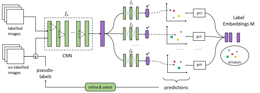
Figure 1: The deep architecture of the proposed progressive ensemble network. The ensemble network consists of multiple ($K$) image classification functions, each of which is a composition of a shared image feature extraction function $f_{v}$ and an individual semantic embedding function $f_{k}$, i.e., $f_{k}\circ f_{v}(x)$, with $k\in\{1,\cdots,K\}$. We use the ResNet-34 [15] as the feature extraction convolutional neural network $f_{v}$ and use a multilayer perceptron with two hidden layers (512 units) and ReLU activation functions as each embedding function $f_{k}$. The progressive training procedure iteratively and dynamically selects unlabeled instances and their predicted pseudo-labels to augment the training data and refine the ensemble network.

3 Approach

We consider zero-shot image recognition in the following setting. We have a set of $N^{s}$ labeled images, $\mathcal{D}_{s}=\{(x_{i},y_{i})\}_{i=1}^{N^{s}}$, from $L^{s}$ seen classes $\mathcal{S}=\{1,\cdots,L^{s}\}$ such that $y_{i}\in\mathcal{S}$. We also have a set of $N^{u}$ images, $\mathcal{D}_{u}=\{(x_{j},y_{j})\}_{j=1}^{N^{u}}$, from $L^{u}$ unseen classes $\mathcal{U}=\{L^{s}+1,\cdots,L\}$ such that $L=L^{s}+L^{u}$, where the labels, $\{y_{j}\in\mathcal{U}\}$, are unavailable during training. We aim to transfer information from the labeled data to predict the labels of the unlabeled instances. To bridge the gap between seen and unseen classes, we also assume we have a semantic label representation matrix $M\in\mathbb{R}^{m\times L}$, e.g., semantic attribute vectors, for all the $L$ seen and unseen classes.

In this section, we present a novel progressive ensemble network model for zero-shot image recognition. The proposed end-to-end framework is depicted in Figure 1. It consists of multiple image classification functions with a shared feature extraction network but different label embedding representations. A progressive training framework is deployed to iteratively refine the overall ensemble network by incorporating unlabeled instances with their predicted pseudo-labels in a dynamic and ensemble manner.

3.1 Ensemble Networks

Following the standard ZSL scheme, we can use a convolutional neural network (CNN) $f_{v}$ to extract high level visual features from an image $x$, and then use an embedding network $f$ to embed the visual features $f_{v}(x)$ into the semantic space, e.g., the attribute space, of label embeddings $\mathbb{R}^{m}$. Here the overall deep network $f\circ f_{v}(x)$ (“$\circ$" denotes a composition operation) forms an image classification function for all classes, $\mathcal{S}\cup\mathcal{U}$, which can categorize an image $x$ to the nearest class in the semantic label embedding space $\mathbb{R}^{m}$. However, though a semantic label embedding matrix $M$ can enable zero-shot information transfer from the seen classes to the unseen classes, the effectiveness of such information transfer can vary substantially for different unseen classes due to their various association levels with the seen classes in the given semantic label embedding space. It is hard to optimize the semantic associations between the seen classes and all unseen classes simultaneously with one fixed label embedding matrix $M$. Hence we propose to project the label embeddings $M$ into $K$ different embedding spaces, $\{\mathcal{P}_{k}:\mathbb{R}^{m}\rightarrow\mathbb{R}^{h}\;|k=1,\cdots,K\}$, to induce $K$ sets of different label embeddings $\{\mathcal{P}_{k}(M)\}$ to facilitate information transfer to the unseen classes. For each label embedding matrix $\mathcal{P}_{k}(M)$, we can produce an embedding network $f_{k}$, e.g., a multilayer perceptron, to map $f_{v}(x)$ into the corresponding label embedding space, which forms a zero-shot classification function $f_{k}\circ f_{v}(x)$. By employing the $K$ classification functions in an ensemble manner we expect the overall ensemble network can effectively reduce the impact of noise and class bias of the original label embeddings $M$ to produce robust zero-shot image recognitions.

3.1.1 Label Embedding Projection

We aim to use different label embeddings to capture different label associations between seen and unseen classes. Towards this goal, we perform the $k$-th label embedding projection $\mathcal{P}_{k}$ adaptively by maximizing the weighted similarity score between the seen classes, $\mathcal{S}$, and a randomly selected subset of the unseen classes, $\mathcal{Z}_{k}\subset\mathcal{U}$, in the projected label embedding space. In particular, we assume a linear projection function $\mathcal{P}_{k}(M)=P^{(k)}M$, where the projection matrix $P^{(k)}\in\mathbb{R}^{h\times m}$ has orthogonal rows, i.e., $P^{(k)}P^{(k)\top}=I$. We formulate the label embedding projection as the following maximization problem:

$$\max_{P^{(k)}} \sum_{i\in\mathcal{S},j\in\mathcal{Z}_{k}}\mbox{tr}(P^{(k)}M_{:i}A_{ij}M_{:j}^{\top}P^{(k)\top})$$ (1)

subject to $$\quad P^{(k)}P^{(k)^{\top}}=I$$

where $M_{:i}$ denotes the $i$-th column of matrix $M$ and tr$(\cdot)$ denotes a trace function, the association weight $A_{ij}$ is defined as the cosine similarity between the corresponding $i$-th and $j$-th classes in the original label representation space. This maximization problem has a closed-form solution:

$$P^{(k)}=[\mathbf{u}_{1},\mathbf{u}_{2},...,\mathbf{u}_{h}]^{\top}$$ (2)

where $\{\mathbf{u}_{i}\}_{i=1}^{h}$ are the top $h$ eigenvectors of matrix $\sum_{i\in\mathcal{S},j\in\mathcal{Z}_{k}}\frac{1}{2}(M_{:i}A_{ij}M_{:j}^{\top}+M_{:j}A_{ij}M_{:i}^{\top})$.

We can produce $K$ different label embedding projection matrices $\{P^{(k)}\}_{k=1}^{K}$ by randomly selecting $K$ different subsets of unseen classes, $\{\mathcal{Z}_{k}\}_{k=1}^{K}$. Each resulting label embedding matrix $P^{(k)}M$ encodes a different knowledge transfer structure between the seen and unseen classes.

3.1.2 Loss Function of the Ensemble Network

Given labeled training instances $\mathcal{D}_{train}=\{(x_{i},y_{i})\}_{i=1}^{N}$, the deep ensemble neural network with $K$ classification functions, $\{f_{k}\circ f_{v}(x)\}_{k=1}^{K}$, can be trained by minimizing the following negative log-likelihood loss function:

$$\mathcal{L}(\omega_{v},\omega_{1},...,\omega_{K})=\frac{1}{N}\sum_{i=1}^{N}\sum_{k=1}^{K}\ell_{k}(\mathbf{v}_{i}^{k},y_{i})$$ (3)

where $(\omega_{v},\omega_{1},...,\omega_{K})$ denote the model parameters, $\mathbf{v}_{i}^{k}=f_{k}\circ f_{v}(x_{i})$ denotes the $k$-th classifier’s prediction vector of instance $x_{i}$ in its label embedding space, and $\ell_{k}(\cdot,\cdot)$ is a negative log-likelihood loss function computed over the softmax prediction scores of the $k$-th classifier:

$$\ell_{k}(\mathbf{v}_{i}^{k},c) =-\mathrm{log}\ p_{k}(c|\mathbf{v}_{i}^{k})$$

$$=-\mathrm{log}\frac{\text{exp}(\mathbf{v}_{i}^{k\top}P^{(k)}M_{:c})}{\sum_{c^{\prime}\in\mathcal{S}\cup\mathcal{U}}\text{exp}(\mathbf{v}_{i}^{k\top}P^{(k)}M_{:c^{\prime}})}$$ (4)

Note the softmax function above is defined over both seen and unseen classes. It is designed to include training instances from both seen and unseen classes. Hence, although initially the labeled training data only contain the labeled instances from the seen classes, such that $\mathcal{D}_{train}=\mathcal{D}_{s}$ and $N=N^{s}$, we will expand it to include pseudo-labeled set from unseen classes through progressive training below.

3.1.3 Ensemble Zero-Shot Prediction

With the multiple classification functions learned in the ensemble network, we can integrate the $K$ classification functions to perform zero-shot prediction on each unlabeled instance $x_{i}$ from unseen classes. We first make predictions using each of the $K$ classifiers based on similarity scores:

$$\hat{y}_{i}^{(k)}=\mathop{\mathrm{arg\ max}}_{c\in\mathcal{Z}_{k}}\quad\langle f_{k}\circ f_{v}(x_{i}),\ P^{(k)}M_{:c}\rangle$$ (5)

where $\langle\cdot,\cdot\rangle$ denotes the inner product of two vectors. As the $k$-th set of label embeddings are produced by maximizing the label associations of seen classes and the subset of unseen classes $\mathcal{Z}_{k}$, we hence only use the $k$-th classifier for zero-shot predictions on the subset of unseen classes $\mathcal{Z}_{k}$. Then we ensemble all the $K$ predictions to determine the predicted class using a normalized majority voting strategy:

$$\hat{y}_{i} =\mathop{\mathrm{arg\ max}}_{c}\quad\phi(x_{i},c)$$ (6)

where $$\phi(x_{i},c)=\frac{\sum_{k=1}^{K}\mathbb{I}{[c=\hat{y}_{i}^{(k)}]}}{\sum_{k=1}^{K}\mathbb{I}{[c\in\mathcal{Z}_{k}]}}$$ (7)

and $\mathbb{I}[\cdot]$ denotes an indicator function that returns value 1 when the given condition is true.

In the case of generalized ZSL, where a test instance $x_{i}$ can be from either a seen or an unseen class, we still compute the voting score of $x_{i}$ belonging to an unseen class $c$ using the normalized voting score in Eq.(7), but we compute the voting score of $x_{i}$ belonging to a seen class $c$ as its average prediction score on this class by all the $K$ classifiers, i.e., $\phi(x_{i},c)=\frac{1}{K}\sum_{k=1}^{K}\langle f_{k}\circ f_{v}(x_{i}),\ P^{(k)}M_{:c}\rangle$.

3.2 Progressive Ensemble Networks

Training with only labeled instances from the seen classes can suffer from the aforementioned domain shift problem. Meanwhile our ensemble network provides a natural foundation for making voting-based predictions on the unseen class instances and incorporating pseudo-labeled instances from the unseen classes in the training process. We hence propose to deploy a progressive training procedure that iteratively and dynamically exploits pseudo-labeled unseen class instances to refine the ensemble network initially trained on the labeled data from seen classes, $\mathcal{D}_{s}$.

The progressive training algorithm is summarized in Algorithm 1. In each iteration, it uses the current ensemble network to predict the pseudo-label $\hat{y}_{i}$ with Equation (6) for each unlabeled instance $x_{i}$ from the unseen classes. Then for each unseen class $c\in\mathcal{U}$, it selects the top $N_{pseudo}$ instances with the largest prediction scores $\phi(x_{i},c)$. The instances selected from all the unseen classes together with their predicted labels form a pseudo-set $\mathcal{D}_{pseudo}=\{(x_{i},\hat{y}_{i})\}_{i=1}^{N_{p}}$. The ensemble network parameters are then refined by minimizing a loss function in Equation (3) over an augmented training set $\mathcal{D}_{train}=\mathcal{D}_{s}\cup\mathcal{D}_{pseudo}$. As the augmented training set contains data from both the seen classes and unseen classes, we expect the refined ensemble network can overcome the domain shift problem in terms of visual appearances of semantic features and improve zero-shot prediction performance. Moreover, instead of gradually increasing the pseudo-set, we dynamically update this set in each iteration with the progressively improved ensemble network to correct potential label mistakes in the previous pseudo-set.

Algorithm 1 Progressive Training of Ensemble Networks

Input: labeled data from seen classes $\mathcal{D}_{s}$, unlabeled data from unseen classes $\mathcal{D}_{u}$, and label embedding matrix $M$.

Initialization:

 $\mathcal{D}_{train}\leftarrow\mathcal{D}_{s}$, $\mathcal{D}_{pseudo}\leftarrow\emptyset$;

 perform label embedding projection for $\{P^{(k)}\}_{k=1}^{K}$;

 train an end-to-end deep ensemble network on $\mathcal{D}_{train}$.

repeat

     predict pseudo-labels of $\mathcal{D}_{u}$ by Eq.(6) and (7);

     generate a pseudo-labeled set $\mathcal{D}_{pseudo}$ by selecting the

   top $N_{pseudo}$ instances from each unseen class;

     update the training set: $\mathcal{D}_{train}\leftarrow\mathcal{D}_{s}\cup\mathcal{D}_{pseudo}$;

     refine the ensemble network parameters on $\mathcal{D}_{train}$.

until $\mathtt{MaxIter}$

4 Experiments

To investigate the empirical performance of our proposed approach, we conducted experiments under both conventional ZSL and generalized ZSL settings. In this section, we present our experimental results and discussions.

4.1 Experiment Settings

4.1.1 Datasets

We used three widely used ZSL datasets with label attribute vectors to conduct experiments. The first one is the Caltech-UCSD-Birds 200-2011 (CUB) dataset [31]. It is a fine-grained dataset of bird species, containing 11,788 images of birds from 200 different species. Each image is also annotated with 312 attributes. The second one is the SUN dataset [23], which contains 14,340 images from 717 different scenes. In this dataset each image is annotated with 102 attributes. The third dataset is the Animal with Attributes 2 (AWA2) dataset [34], which is an updated version of the previous AWA [20] dataset. AWA2 consists of 37,322 images from 50 animal classes. It also provides 85 numerical attribute values for each class. We used AWA2 instead of AWA as the raw image data of AWA is not publicly available any more. Following previous ZSL works, we extracted the label embedding matrix $M$ from the attribute vectors.

4.1.2 Seen/Unseen Splits

In order to perform ZSL, a dataset needs to be split into two disjoint subsets, the seen classes $\mathcal{S}$ and the unseen classes $\mathcal{U}$. To perform scientific ZSL study and maintain the ‘zero-shot’ principle, a ZSL model should never have access to the true label information of the unseen class instances during the training phase. However many ZSL approaches have used CNN models pre-trained on the ImageNet [25] for image feature extraction. If the pre-trained ImageNet classes have overlaps with the ZSL test classes, it should be considered as violating the ‘zero-shot’ rule. As pointed out in the comprehensive evaluation study [34], standard splits (SS) on the ZSL datasets have unseen class overlaps with the 1K classes of ImageNet, which can lead to superior performance on these classes. Therefore in this study we also used the ZSL splits proposed in [34] (PS), which has the same number of test classes as the SS splits but ensures no class in ImageNet appears in the test set of ZSL. For the SUN dataset, except for the split with 72 test classes, there is another split with 10 test classes from [16], which is also used in some previous works. We denote this split as SUN10 and the split with 72 test classes as SUN72. The overview of these datasets and seen/unseen class splits are summarized in Table 1.

Table 1: Summary of three attribute datasets for ZSL.

Dataset	Images	Avg.	Classes	Attr.
CUB	11788	$\sim$60	200 (150+50)	312
SUN	14340	$\sim$20	717 (645+72)	102
AWA2	37322	$\sim$750	50 (40+10)	85

Table 2: Conventional ZSL results. $\dagger$ denotes numbers cited from [34]. Methods in the top part of the table reported the Top-1 accuracy results (TOP-1), while those in the bottom part reported the multi-class accuracy (MACC) results. Numbers in bracket denote results on AWA instead of AWA2. Best results are shown in bold font and second best in italic font.

	Methods	CUB		AWA2		SUN72		SUN10
		SS	PS	SS	PS	SS	PS
Top-1	DeViSE [10]$\dagger$	53.2	52.0	68.6	59.7	57.5	56.5	-
	SynC [8]$\dagger$	54.1	55.6	71.2	46.6	59.1	56.3	-
	ALE [1]$\dagger$	53.2	54.9	80.3	62.5	59.1	58.1	-
	SJE [2]$\dagger$	55.3	53.9	69.5	61.9	57.1	53.7	-
	SAE [19]$\dagger$	33.4	33.3	80.7	54.1	42.4	40.3	-
	ReViSE [29]	65.4	-	(93.4)	-	-	-	-
	GFZSL [30]	63.8	-	(94.3)	-	-	-	87.0
	QFSL [28]	69.7	72.1	84.8	79.7	61.7	58.3	-
	Progressive Training	54.0	49.8	73.2	57.8	49.6	47.9	76.6
	PrENw/oProj	64.7	61.4	88.5	66.6	61.1	60.1	84.4
	PrEN (proposed)	66.9	66.4	95.7	74.1	63.3	62.9	86.3
mAcc	UDA [18]	40.6	-	(75.6)	-	-	-	-
	DCL [13]	-	-	(81.9)	-	-	-	84.4
	Progressive Training	53.7	49.9	73.0	53.8	49.5	48.0	76.7
	PrENw/oProj	64.4	61.4	89.4	65.7	61.0	60.2	84.5
	PrEN (proposed)	66.6	66.4	96.1	78.6	63.2	62.8	86.4

4.1.3 Evaluation Metric

We adopted the popularly used Top-1 accuracy to evaluate the ZSL prediction performance. The Top-1 accuracy counts the proportion of correctly labeled instances in each test class and then takes an average over all these classes. To compare with some literature works, we also reported the multi-class classification accuracy results when needed.

4.1.4 Implementation Details

For an input image, we resized it to $224\times 224$ and fed it to ResNet-34 [15]. The 512 dimensional vector from the last average pooling layer of ResNet is used as visual features of the image. The ResNet is initialized by the pre-trained model on ImageNet. We used multilayer perceptrons (MLPs) with two hidden layers (each with size 512) and one output layer (with size $h$) as the consequent embedding functions. ReLU activation is applied after each layer. We used Adam [17] to train our model, with the default parameter setting $\beta_{1}=0.9$, $\beta_{2}=0.999$ and learning rate $\eta=0.001$. We set $\mathtt{MaxIter}=20$. In each iteration the model is trained with 100 batches with batch size 64. For the progressive training procedure, we used $N_{pseudo}=\mathtt{min}(\rho N_{avg},N_{max})$, where $N_{avg}$ is the average number of images in each training class, $\rho$ and $N_{max}$ are set to 0.25 and 20 respectively. We used $K=50$ different label embeddings (i.e., the number of classifiers). For $\{\mathcal{Z}_{k}\}_{k=1}^{K}$, which are the randomly selected subsets of unseen classes for producing the label embedding projection matrices, we set the size of each $\mathcal{Z}_{k}$ as half of the unseen class number. We projected the original label embeddings to a lower dimension space such $h<m$. We used h=70 in the experiments if not specifically noted.

4.2 Conventional ZSL Results

4.2.1 Comparison Methods

We compared the proposed Progressive Ensemble Network (PrEN) model with a number of state-of-the-art ZSL methods. These methods can be divided into two groups: DeViSE [10], SynC [8], ALE [1], SJE [2], and SAE [19] belong to inductive ZSL methods, while the transductive methods include UDA [18], DCL [13], ReViSE [29], GFZSL [30], and QFSL [28]. All the comparison methods used the standard fixed splits. We hence take the convenience to cite the results from [34] and the literature for fair comparisons.

In order to separate the impact of the progressive training principle from our proposed ensemble framework, we also compared with a Progressive Training baseline variant of the proposed model, which drops the ensemble framework to use only one classifier with the original label embeddings. Moreover, to investigate the effectiveness of multiple adaptive label embedding projections, we also tested another ensemble baseline variant, which deviates from the proposed model only by using the same original label embeddings for the $K$ classifiers without any projection. We denote this baseline variant as PrEN_w/oProj.

4.2.2 Result Analysis

We summarized the comparison results in Table 2. As two different evaluation metrics, Top-1 Accuracy and multi-class accuracy, are used in the comparison works, we divide the table into two parts, where the top part presents Top-1 accuracy results and the bottom part presents multi-class accuracy results. We reported the results of our proposed PrEN method in terms of both evaluation metrics. From the table, we notice that most results under ‘PS’ are worse than their counterpart results under ‘SS’, especially on the AWA2 datasets. This indicates that the overlapping of test classes with ImageNet 1K classes did bring extra benefit in performance. However, the transductive ZSL methods we found are mostly evaluated under the ‘SS’ setting, we hence expect their missing results under ‘PS’ can only be worse than the reported ‘SS’ results. Moreover, the transductive works, ReViSE, GFZSL, UDA and DCL, reported results on CUB, AWA or SUN10, but not on AWA2 and SUN72. Since AWA2 is nearly a drop-in-replacement of AWA [34], we included their results on AWA just for reference.

From the comparison results in terms of Top-1 accuracy, we can see that PrEN outperforms all the five inductive methods across all datasets. Comparing with the transductive methods, PrEN produced the second best results on CUB, SUN10, and the ‘PS’ split of AWA2, where QFSL performs the best. Nevertheless, PrEN produced the best results in all the other cases, the ‘SS’ split of AWA2, both ‘SS’ and ‘PS’ splits of SUN72. In particular, on the more challenging scene classification dataset SUN72 (more unseen classes and less training data for each class), PrEN achieves 63.3% and 62.9% on ‘SS’ and ‘PS’ splits, and outperforms all the other methods with notable performance gains. In terms of multi-class accuracy, our proposed PrEN largely outperforms the two transductive ZSL methods, UDA and DCL. For example, PrEN achieves 66.6% on CUB and 86.4% on SUN10, which are much better than the 40.6% reported by UDA on CUB and the 84.4% reported by DCL on SUN10 respectively. These results demonstrate the efficacy of the proposed approach for conventional zero-shot image recognition tasks.

By comparing the proposed PrEN with the baseline variants, we notice there are large performance gaps between the proposed full model PrEN and the two variants, Progressive-Training baseline variant and PrEN_w/oProj. Without the ensemble architecture and the diverse label embeddings, the progressive training procedure alone cannot produce any effective model. Even by just dropping the label embedding projection but maintaining the ensemble architecture, PrEN_w/oProj still yields much inferior performance than PrEN. These suggest that the proposed ensemble network architecture with the essential label embedding projections forms a solid and critical foundation for incorporating pseudo-labels through progressive training.

Table 3: Generalized ZSL results in terms of average Top-1 accuracy. $\dagger$ denotes numbers cited from [34]. ‘u’ and ‘s’ denotes Top-1 accuracies on unseen and seen classes, respectively. ‘H’ denotes the harmonic mean of them.

Methods	CUB			AWA2			SUN72
	u	s	H	u	s	H	u	s	H
DeViSE [10]$\dagger$	23.8	53.0	32.8	17.1	74.7	27.8	16.9	27.4	20.9
SynC [8]$\dagger$	11.5	70.9	19.8	10.0	90.5	18.0	7.9	43.3	13.4
ALE [1]$\dagger$	23.7	62.8	34.4	16.8	76.1	27.5	21.8	33.1	26.3
SJE [2]$\dagger$	23.5	59.2	33.6	8.0	73.9	14.4	14.7	30.5	19.8
SAE [19]$\dagger$	7.8	54.0	13.6	1.1	82.2	2.2	8.8	18.0	11.8
PrEN (proposed)	35.2	55.8	43.1	32.4	88.6	47.4	35.4	27.2	30.8

Empirical Computational Complexity.

From above, we can see that tremendous performance gain has been achieved by the proposed PrEN model over its baseline Progressive Training variant. As PrEN involves training multiple classifiers, $K=50$ in our experiments, while the Progressive Training variant has $K=1$, a natural question to ask is that how much additional computational cost is required to yield such performance gain. Here we use the number of floating-point operations (FLOPs), i.e., the total number of multiplication and addition operations, involved in passing one image from the input of the deep network architecture to the outputs as an empirical measure of the computational complexity induced by each deep model. Both models share the same ResNet34 backbone structure which involves 3.6 billion FLOPs, while PrEN has 49 more MLP components than the Progressive baseline, and each component has around 0.8 million FLOPs. Comparing to the 3.6 billion FLOPs in the backbone ResNet, the additional 49$\times$0.8 million $\approx$ 0.04 billion FLOPs induced by the proposed PrEN is relatively negligible, which however contributed to the average $16.9\%$ and $17.9\%$ performance gain in terms of Top-1 accuracy and multi-class accuracy respectively. This again validates the suitability and efficacy of the proposed ensemble architecture with localized adaptive label embedding projections.

4.3 Parameter Sensitivity Analysis

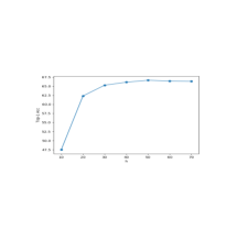
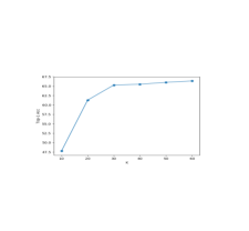
Figure 2: Parameter sensitivity analysis.

In this section, we investigate the sensitivity of the proposed model with respect to its two hyper-parameters, $K$ and $h$. $K$ is the number of projected label embeddings as well as the number of classifiers, while $h$ is the dimension of projected label embeddings.

To study how does $h$ affect the test performance, we performed conventional ZSL on the CUB dataset with the ‘PS’ split. We fixed $K=50$ and repeated the experiment for each $h$ value from the set $\{10,20,30,...,70\}$. The test accuracies are reported on the left side of Figure 2. We can see that the test ZSL accuracies increase quickly from $h=10$ to $h=30$ and then the increase becomes very small. Nevertheless the best performance is achieved at $h=50$. This suggests that larger dimension does help preserve useful information in the projected label embeddings. But even with a very small fraction of the original dimension, e.g., 10%, our model can achieve very good performance; on CUB a $h$ value within $(30,70]$ would be a safe choice.

We also performed sensitivity analysis for $K$ on CUB. We fixed $h=70$ and tested different $K$ values from $\{10,20,...,60\}$. The test accuracy results with different $K$ values are reported in the right subfigure of Figure 2. It is easy to observe that the ZSL accuracy is very poor when $K$ has a small value $10$. Then the ZSL performance dramatically increases with $K$ increasing from 10 to 30, and the change becomes very small with $K$ further increasing to 60. These results suggest our proposed model is not very sensitive to the hyper-parameters $K$ as long as it is set to values within the reasonable range, such as $K>30$.

4.4 Generalized ZSL Results

Majority of ZSL works in the literature has focused on the conventional ZSL setting, where the test classes are assumed to consist of only unseen classes. This assumption can be overly strict. Hence here we conducted experiments to compare the test performance of the proposed progressive ensemble network (PrEN) with related methods under the generalized ZSL (GZSL) setting, where the test instances can come from both seen and unseen classes. As the classifiers within our PrEN model perform multi-class classification over all the classes, it can be conveniently extended to address GZSL. For GZSL the main problem is that many unseen class instances can be wrongly classified into seen classes. Hence we only select pseudo instances for unseen classes in the first few iterations of the progressive training process, while selecting pseudo instances for both seen and unseen classes in later iterations to achieve balanced performance. To evaluate our model under GZSL, we follow the comprehensive study in [34] to use the ‘PS’ splits, and separate a random 20% of the instances for each seen class and add these into the test set. We evaluated the top-1 test accuracy on unseen and seen classes separately, and compute their harmonic mean as the GZSL accuracy result. We compared to five ZSL methods that have addressed GZSL in the literature. Although the authors of [28] also reported their GZSL results of the transductive method QFSL, they conducted GZSL in a non-standard and limited general setting with extra knowledge – they assumed whether the unlabeled instances belong to seen vs unseen classes is known. For fairness, we hence did not compare with their results. Our comparison results are reported in Table 3.

We can see that some comparison methods can achieve quite good performance on seen classes while their zero-shot accuracy on unseen classes is very low; for example SynC achieves 11.5% (unseen) and 70.9% (seen) on AWA2 , as well as 10.0% (unseen) and 90.5% (seen) on CUB. The overall performance of the comparison methods on all classes, under column ‘H’, is still poor. We also notice there is usually a trade-off between the performance on the seen classes and that on the unseen classes, while the harmonic mean measures the overall performance. The proposed PrEN though didn’t yield superior performance on seen classes, its zero-shot prediction performance on unseen classes is much better than the other comparison methods. Moreover, in terms of the overall GZSL performance, we can see the proposed PrEN outperforms all the comparison methods with large margins. This validates the effectiveness of the proposed model under GZSL setting.

5 Conclusion

In this paper, we proposed a novel progressive deep ensemble network for transductive zero-shot image recognition. By integrating multiple classifiers with different label embeddings, the ensemble network can maintain informative knowledge transfer from seen classes to unseen classes through adaptive inter-label relations. By progressively refining the ensemble network parameters with pseudo-labeled test instances, the training procedure can alleviate the domain shift problem and avoid overfitting to the seen classes. We conducted experiments on multiple standard datasets under both conventional and generalized ZSL settings. The proposed model has demonstrated superior performance than the state-of-the-art comparison methods.

References

- [1] Z. Akata, F. Perronnin, Z. Harchaoui, and C. Schmid. Label-embedding for attribute-based classification. In CVPR, 2013.
- [2] Z. Akata, S. Reed, D. Walter, H. Lee, and B. Schiele. Evaluation of output embeddings for fine-grained image classification. In CVPR, 2015.
- [3] J. Ba, K. Swersky, S. Fidler, et al. Predicting deep zero-shot convolutional neural networks using textual descriptions. In ICCV, 2015.
- [4] Y. Bengio, J. Louradour, R. Collobert, and J. Weston. Curriculum learning. In ICML, 2009.
- [5] A. Blum and T. Mitchell. Combining labeled and unlabeled data with co-training. In COLT, 1998.
- [6] M. Bucher, S. Herbin, and F. Jurie. Improving semantic embedding consistency by metric learning for zero-shot classiffication. In ECCV, 2016.
- [7] M. Bucher, S. Herbin, and F. Jurie. Generating visual representations for zero-shot classification. In ICCV Workshops: TASK-CV: Transferring and Adapting Source Knowledge in Computer Vision, 2017.
- [8] S. Changpinyo, W.-L. Chao, B. Gong, and F. Sha. Synthesized classifiers for zero-shot learning. In CVPR, 2016.
- [9] S. Changpinyo, W.-L. Chao, and F. Sha. Predicting visual exemplars of unseen classes for zero-shot learning. In ICCV, 2017.
- [10] A. Frome, G. S. Corrado, J. Shlens, S. Bengio, J. Dean, T. Mikolov, et al. Devise: A deep visual-semantic embedding model. In NIPS, 2013.
- [11] Y. Fu, T. M. Hospedales, T. Xiang, and S. Gong. Transductive multi-view zero-shot learning. IEEE TPAMI, 37(11):2332–2345, 2015.
- [12] Y. Fu, T. M. Hospedales, T. Xiang, and S. Gong. Transductive multi-view zero-shot learning. TPAMI, 37(11):2332–2345, 2015.
- [13] Y. Guo, G. Ding, J. Han, and Y. Gao. Zero-shot recognition via direct classifier learning with transferred samples and pseudo labels. In AAAI, 2017.
- [14] Y. Guo, G. Ding, X. Jin, and J. Wang. Transductive zero-shot recognition via shared model space learning. In AAAI, 2016.
- [15] K. He, X. Zhang, S. Ren, and J. Sun. Deep residual learning for image recognition. In CVPR, 2016.
- [16] D. Jayaraman and K. Grauman. Zero-shot recognition with unreliable attributes. In NIPS, 2014.
- [17] D. P. Kingma and J. Ba. Adam: A method for stochastic optimization. In ICLR, 2015.
- [18] E. Kodirov, T. Xiang, Z. Fu, and S. Gong. Unsupervised domain adaptation for zero-shot learning. In CVPR, 2015.
- [19] E. Kodirov, T. Xiang, and S. Gong. Semantic autoencoder for zero-shot learning. In CVPR, 2017.
- [20] C. H. Lampert, H. Nickisch, and S. Harmeling. Learning to detect unseen object classes by between-class attribute transfer. In CVPR, 2009.
- [21] F. Ma, D. Meng, Q. Xie, Z. Li, and X. Dong. Self-paced co-training. In ICML, 2017.
- [22] M. Norouzi, T. Mikolov, S. Bengio, Y. Singer, J. Shlens, A. Frome, G. S. Corrado, and J. Dean. Zero-shot learning by convex combination of semantic embeddings. In ICLR, 2014.
- [23] G. Patterson, C. Xu, H. Su, and J. Hays. The sun attribute database: Beyond categories for deeper scene understanding. IJCV, 108(1-2):59–81, 2014.
- [24] B. Romera-Paredes and P. H. Torr. An embarrassingly simple approach to zero-shot learning. In ICML, 2015.
- [25] O. Russakovsky, J. Deng, H. Su, J. Krause, S. Satheesh, S. Ma, Z. Huang, A. Karpathy, A. Khosla, M. Bernstein, A. C. Berg, and L. F.-F. ImageNet Large Scale Visual Recognition Challenge. IJCV, 115(3):211–252, 2015.
- [26] K. Saito, Y. Ushiku, and T. Harada. Asymmetric tri-training for unsupervised domain adaptation. In ICML, 2017.
- [27] R. Socher, M. Ganjoo, C. D. Manning, and A. Ng. Zero-shot learning through cross-modal transfer. In NIPS, 2013.
- [28] J. Song, C. Shen, Y. Yang, Y. Liu, and M. Song. Transductive unbiased embedding for zero-shot learning. In CVPR, 2018.
- [29] Y.-H. H. Tsai, L.-K. Huang, and R. Salakhutdinov. Learning robust visual-semantic embeddings. In ICCV, 2017.
- [30] V. Verma and P. Rai. A simple exponential family framework for zero-shot learning. In ECML, 2017.
- [31] C. Wah, S. Branson, P. Welinder, P. Perona, and S. Belongie. The Caltech-UCSD Birds-200-2011 Dataset. Technical Report CNS-TR-2011-001, California Institute of Technology, 2011.
- [32] Y. Wu, Y. Lin, X. Dong, Y. Yan, W. Ouyang, and Y. Yang. Exploit the unknown gradually: One-shot video-based person re-identification by stepwise learning. In CVPR, 2018.
- [33] Y. Xian, Z. Akata, G. Sharma, Q. Nguyen, M. Hein, and B. Schiele. Latent embeddings for zero-shot classification. In CVPR, 2016.
- [34] Y. Xian, C. H. Lampert, B. Schiele, and Z. Akata. Zero-shot learning-a comprehensive evaluation of the good, the bad and the ugly. arXiv preprint arXiv:1707.00600, 2017.
- [35] L. Zhang, T. Xiang, and S. Gong. Learning a deep embedding model for zero-shot learning. In CVPR, 2017.
- [36] Z.-H. Zhou and M. Li. Tri-training: Exploiting unlabeled data using three classifiers. IEEE TKDE, 17(11):1529–1541, 2005.
- [37] Y. Zhu, M. Elhoseiny, B. Liu, and A. Elgammal. Imagine it for me: Generative adversarial approach for zero-shot learning from noisy texts. arXiv preprint arXiv:1712.01381, 2017.