Butterfly-Net: Optimal Function Representation Based on Convolutional Neural Networks

Abstract

Deep networks, especially convolutional neural networks (CNNs), have been successfully applied in various areas of machine learning as well as to challenging problems in other scientific and engineering fields. This paper introduces Butterfly-net, a low-complexity CNN with structured and sparse cross-channel connections, together with a Butterfly initialization strategy for a family of networks. Theoretical analysis of the approximation power of Butterfly-net to the Fourier representation of input data shows that the error decays exponentially as the depth increases. Combining Butterfly-net with a fully connected neural network, a large class of problems are proved to be well approximated with network complexity depending on the effective frequency bandwidth instead of the input dimension. Regular CNN is covered as a special case in our analysis. Numerical experiments validate the analytical results on the approximation of Fourier kernels and energy functionals of Poisson’s equations. Moreover, all experiments support that training from Butterfly initialization outperforms training from random initialization. Also, adding the remaining cross-channel connections, although significantly increase the parameter number, does not much improve the post-training accuracy and is more sensitive to data distribution.

1 Introduction

Deep neural network is a central tool in machine learning and data analysis nowadays [5]. In particular, convolutional neural network (CNN) has been proved to be a powerful tool in image recognition and representation. Deep learning has also emerged to be successfully applied in solving PDEs [6, 28, 37] and physics problems [4, 17, 35, 47, 53], showing the potential of becoming a tool of great use for computational mathematics and physics as well. Given the wide application of PDEs and wavelet based methods in image and signal processing [8, 11, 39], an understanding of CNN’s ability to approximate differential and integral operators will lead to an explanation of CNN’s success in these fields, as well as possible improved network architectures.

The remarkable performance of deep neural networks across various fields relies on their ability to accurately represent functions of high-dimensional input data. Approximation analysis has been a central topic to the understanding of the neural networks. The classical theory developed in 80’s and early 90’s [3, 13, 26] approximates a target function by a linear combination of sigmoids, which is equivalent to a fully connected neural network with one hidden layer. While universal approximation theorems were established for such shallow networks, the research interest in neural networks only revived in recent years after observing the successful applications of deep neural networks, particular the superior performance of CNNs in image and signal processing.

Motivated by the empirical success, the approximation advantage of deep neural networks over shallow ones has been theoretically analyzed in several places. However, most results assume stacked fully connected layers and do not apply to CNNs which have specific geometrical constraints: (1) the convolutional scheme, namely local-supported filters with weight sharing, and (2) the hierarchical multi-scale architecture. The approximation power of deep networks with hierarchical geometrically-constrained structure has been studied recently [12, 40, 41], yet the network architecture differ from the regular CNN. The approximation theory of CNN has been studied in [2, 54]. We review the related literature in more detail below.

Figure 1: Illustration of a Butterfly-net: The network consists of 3 modules, (1) Conv layers, which has one Interpolation later and $L_{t}$ Recursion layers, (2) A Switch layer, and (3) Conv-t layers, which has $L_{\xi}$ Recursion layers and one Interpolation later. The conv and conv-t layers have convolutional and transpose convolutional structure respectively, and the Switch layer only involves local operations. Detailed structures of these layers are given in Section 3. This figure shows the case when $L_{t}=L_{\xi}=2$, and the notations $V,H^{(\ell)},M,G^{(\ell)},U$ denote the matrix representations of the operations in the scheme, c.f. Section 3.4. The name “butterfly” can be understood from the shape of the network.

This paper proposes a specific architecture under the CNN framework based on the Butterfly scheme originally developed for the fast computation of special function transforms [42, 44, 52] and Fourier integral operators [9, 10, 31, 32, 33, 34]. Butterfly scheme provides a hierarchical structure with locally low-rank interpolation of kernel functions and can be applied to solve many PDE related problems. In terms of computational complexity, the scheme is near optimal for Fourier kernels and Fourier integral operators. The proposed Butterfly-net explicitly adopts the hierarchical structure in Butterfly scheme as the stacked convolutional layers. If the parameters are hard-coded as that in the Butterfly scheme (Butterfly initialization), then Butterfly-net collectively computes the Fourier coefficients of the input signal with guaranteed numerical accuracy. Unlike regular CNN which has dense cross-channel connections, the channels in the Butterfly-net have clear correspondences to the frequency bands, namely the position in the spectral representation of the signal, and meanwhile, the cross-channel weights are sparsely connected. In this paper, we also study Butterfly-net with dense cross-channel connections, which is named Inflated-Butterfly-net. Regular CNN is a special Inflated-Butterfly-net [49]. Comparing Butterfly-net and Inflated-Butterfly-net, Butterfly-net is much lighter: the model complexity (in terms of parameter number) is $O(K\log N)$ and computational complexity is $O(N\log N)$, where $N$ is the length of the discrete input signal and $K$ is the frequency bandwidth.

The approximation error of Butterfly-net in representing Fourier kernels is proved to exponentially decay as the network depth increases, which is numerically validated in Section 5. Due to the efficient approximation of Fourier kernels, Butterfly-net thus possesses all approximation properties of the Fourier representation of input signals, which is particularly useful for solving PDEs and (local) Fourier-based algorithms in image and signal processing. Theoretically, the approximation guarantee for Butterfly-net to represent Fourier kernels leads to an approximation result of a family of sparsified CNNs and regular CNNs. The informal statement of our main result on neural network function approximation is as follows:

Theorem 1.1 (Informal version).

Consider using neural network to approximate a function $f(\vec{x})$, $\vec{x}\in\mathcal{X}\subset\mathbb{R}^{n}$, where $f$ can be approximated by a band-limited function of $\vec{x}$ with bandwidth $K$ (this may be due to the frequency decay of $f$, or $\mathcal{X}$, or both). Then there exists a family of Butterfly-nets whose numbers of parameters are all bounded by

$$n_{b}\lesssim K\log N,$$ (1)

such that using anyone of them to extract a deep feature of length $K$ from the input $x$ can reduce the effective dimension of the input data from $N$ to $K$ for neural network function approximation.

The dimension reduction is reflected by the needed network complexity in approximating $f(\vec{x})$ by a fully-connected network, namely a reduction from a factor of $\varepsilon^{-N/s}$ (for a fully connected net to approximate $f(\vec{x})$ directly) to that of $\varepsilon^{-K/s}$ (for a fully connected net to approximate $g$, Butterfly-net to approximate $\mathcal{B}$, and $f(\vec{x})\approx g(\mathcal{B}\vec{x})$), where $s$ is the regularity level and $\varepsilon$ is the uniform approximation error of $f$. The precise statement is given in Theorem 4.4.

Moreover, in the above statement, the family of Butterfly-nets can be replaced by the corresponding family of Inflated-Butterfly-net with $n_{b}\lesssim K^{2}\log N$ parameters and the same dimension reduction argument still holds. In particular, one member in the family of Inflated-Butterfly-nets is a regular CNN. Hence, our approximation analysis covers regular CNNs as a special case.

1.1 Contributions

Our contributions can be summarized as follows.

1. We propose a family of novel neural network architectures, named Butterfly-nets, which are composed of convolutional and transpose convolutional layers with sparse cross-channel connections, plus a locally connected switch layer in between. An associated Butterfly initialization strategy is proposed for Butterfly-nets to approximate Fourier kernels. The Butterfly-net architecture can be inflated via replacing the sparse cross-channel connections by dense connections, and this contains regular CNN as a special case.

2. The approximation error of Butterfly-nets representing the Fourier kernels is theoretically proved to be exponentially decay as the network depth increases. Concatenating Butterfly-net (or its inflated version) with a fully-connected layer, we provide an approximation analysis for a wide class of functions with frequency decay property and the approximation complexity depends on the effective dimension $K$ instead of the input data dimension $N$. The regular CNN is covered as a special case.

3. Numerically, we apply Butterfly-net and its inflated version to a wide range of datasets. The successful trainings on all datasets support our approximation analysis. Further, we find that training from Butterfly initialization in all cases outperforms training from random initialization, especially when the output function only depends on a few frequencies among the wide frequency band of the input data. Butterfly-net achieves similar post-training accuracy as its inflated version with far less number of parameters. Butterfly-net also admits better transfer learning capability when the distribution of the testing data is shifted away from the training data.

1.2 Related Works

Before we explain more details in the rest of the paper, we review some related works.

Fast algorithm inspired neural network structures. Fast algorithm has inspired several neural network structures recently. Based on $\mathcal{H}$-matrix and $\mathcal{H}^{2}$-matrix structure, Fan and his coauthors proposed two multiscale neural networks [20, 21], which are more suitable in training smooth linear or nonlinear operators due to the multiscale nature of $\mathcal{H}$-matrices. In addition to that, nonstandard wavelet form inspired the design of BCR-Net [22], which is applied to address the inverse of elliptic operator and nonlinear homogenization problem and recently been embedded in a neural network for solving electrical impedance tomography [19] and pseudo-differential operator [23]. Multigrid method also inspired MgNet [25]. In addition to the above approximation of relatively smooth operators, Butterfly scheme inspired the design of SwitchNet [27], which is a non-convolutional three layer neural network and addresses scattering problems.

Classical approximation results of neural networks. Universal approximation theorems for fully-connected neural networks with one hidden layer were established in [13, 26] showing that such networks can approximate a target function with arbitrary accuracy if the hidden layer is allowed to be wide enough. In theory, the family of target functions can include all measurable functions [26], when exponentially many hidden neurons are used. Gallant and White [24] proposed “Fourier network”, proving universal approximation to squared-integrable functions by firstly constructing a Fourier series approximation of the target function in a hard-coded way. These theorems are firstly proved for one-dimensional input, and when generalizing to the multivariate case the complexity grows exponentially.

Using the Fourier representation of the target function supported on a sphere in $\mathbb{R}^{d}$, Barron [3] showed that the mean squared error of the approximation, integrated with arbitrary data distribution on the sphere, decays as $O(n^{-1})$ when $n$ hidden nodes are used in the single hidden layer. The results for shallow networks are limited, and the approximation power of depth in neural networks has been advocated in several recent works, see below. Besides, while the connection to Fourier analysis was leveraged, at least in [3, 24], it is different from the hierarchical function representation scheme as what we consider here.

Approximation power of deep neural networks. The expressive power of deep neural networks has drawn many research interests in recent years. The approximation power of multi-layer restricted Boltzmann machines (RBM) was studied in [30], which showed that RBMs are universal approximators of discrete distributions and more hidden layers improves the approximation power. Relating to the classical approximation results in harmonic analysis, Bölcskei et al. [7] derived lower bounds for the uniform approximation of square-integrable functions, and proved the asymptotic optimality of the sparsely connected deep neural networks as a universal approximator. However, the network complexity also grows exponentially when the input dimension increases.

The approximation advantage of deep architecture over shallow ones has been studied in several works. Delalleau and Bengio [14] identified a deep sum-product network which can only be approximated by an exponentially larger number of shallow ones. The exponential growth of linear regions as the number of layers increases was studied in [43, 48]. Eldan and Shamir [18] constructed a concrete target function which distinguishes three and two-layer networks. Liang and Srikant [36] showed that shallow networks require exponentially more neurons than deep networks to obtain a given approximation error for a large class of functions. The advantage of deep ReLU networks over the standard single-layer ones was analyzed in [51] in the context of approximation in Sobolev spaces. Lu et al. [38] shows the advantage of deep ReLU networks in approximating smooth (band-limited) functions. The above works address deep networks with fully-connected layers, instead of having geometrically-constrained constructions like CNNs.

Deep neural networks with such geometric constraints are relatively less analyzed. The approximation power of a hierarchical binary tree network was studied in [40, 41] which supports the potential advantage of deep CNNs. Cohen et al. [12] used convolutional arithmetic circuits to show the equivalence between a deep network and a hierarchical Tucker decomposition of tensors, and proved the advantage of depth in function approximation. The networks being studied differ from the regular CNNs widely used in the typical real world applications. Recently, Zhou [54] proposed the universal approximation theory of deep CNN with an estimation on the number of free parameters. Bao et al. [2] shows the approximation power of CNNs over deep neural networks without constraints on a class of functions. Comparing to [54], our analysis covers a wider range of networks and the approximation complexity is much lower on a restricted function class. Comparing to [2], different function classes are discussed and we both show the advantage of CNN.

1.3 Organization

The rest of this paper is organized as follows. Building on top of the traditional Butterfly literature, Section 2 first shows the low-rank property of Fourier kernel and illustrates the Butterfly algorithm tailored for Fourier kernel. Section 3 proposes interpolative convolutional layer as building blocks for Butterfly-net followed by the Butterfly-net architecture with Butterfly initialization and its matrix representation. Section 4 analyzes the approximation power of Butterfly-net on Fourier kernels and its extension to general functionals. Numerical results of Butterfly-net and Inflated-Butterfly-net are presented in Section 5 including the performance comparison of network architectures, initializations, and datasets. Finally, in Section 6, we conclude the paper together with discussion on future directions.

2 Preliminaries

This section paves the path to Butterfly-net. We first derives a low-rank interpolation of the Fourier kernel, which is crucial to the efficiency of Butterfly scheme and Butterfly-net. Then in Section 2.2, we reviews the Butterfly algorithm for Fourier kernel. Readers, who are familiar with butterfly scheme, should be safe to skip it.

2.1 Low-rank Approximation of Fourier Kernel

Fourier kernel throughout this paper is defined as,

$$\mathcal{K}(\xi,t)=e^{-2\pi\imath\xi\cdot t},\qquad\xi\in[K_{0},K_{0}+K),\quad t\in[0,1),$$ (2)

where $[K_{0},K_{0}+K)$ denotes the frequency window of interests, $K_{0}$ denotes the starting frequency, and $K$ denotes the frequency window width. It is well-known that the discrete Fourier transform (DFT) matrix, i.e., uniform discretization of (2) with proper scaling, has orthonormal rows and columns. Hence, the DFT matrix is a unitary matrix of full rank and the Fourier kernel is also full rank. Theorem 2.1 show when the Fourier kernel is restricted to certain pairs of subdomains of $[0,1)$ and $[K_{0},K_{0}+K)$, it has low-rank property.

We first give a brief introduction of the Chebyshev interpolation with $r$ points. The Chebyshev grid of order $r$ on $[-\frac{1}{2},\frac{1}{2}]$ is defined as,

$$\left\{z_{i}=\frac{1}{2}\cos\left(\frac{(i-1)\pi}{r}\right)\right\}_{i=1}^{r}.$$ (3)

The Chebyshev interpolation of a function $f(x)$ on $[-\frac{1}{2},\frac{1}{2}]$ is defined as,

$$\Pi_{r}f(x)=\sum_{k=1}^{r}f(z_{k})\mathcal{L}_{k}(x),$$ (4)

where $\mathcal{L}_{k}(x)$ is the Lagrange polynomial as,

$$\mathcal{L}_{k}(x)=\prod_{p\neq k}\frac{x-z_{p}}{z_{k}-z_{p}}.$$ (5)

Several earlier works [9, 10, 33] proved the Chebyshev interpolation representation for Fourier integral operators, which are generalized Fourier kernel. Theorem 2.1 is a special case of these earlier work but with more precise and explicit estimation on the prefactor.

Theorem 2.1.

Let $r$ be the number of Chebyshev points, $B\subset[0,1)$ and $A\subset[K_{0},K_{0}+K)$ denote a domain pair such that $w(A)w(B)\leq\frac{r}{\pi e}$, where $w(\cdot)$ is the domain length function. Then there exists low-rank representations of the Fourier kernel restricted to the domain pair,

$$\sup_{\xi\in A,t\in B}\absolutevalue{\,e^{-2\pi\imath\xi\cdot t}-\sum_{k=1}^{r}e^{-2\pi\imath\xi\cdot t_{k}}e^{-2\pi\imath\xi_{0}\cdot\left(t-t_{k}\right)}\mathcal{L}_{k}(t)\,}\leq\left(2+\frac{2}{\pi}\ln r\right)\left(\frac{\pi ew(A)w(B)}{2r}\right)^{r},$$ (6)

and

$$\sup_{\xi\in A,t\in B}\absolutevalue{\,e^{-2\pi\imath\xi\cdot t}-\sum_{k=1}^{r}e^{-2\pi\imath\left(\xi-\xi_{k}\right)\cdot t_{0}}\mathcal{L}_{k}(\xi)e^{-2\pi\imath\xi_{k}\cdot t}\,}\leq\left(2+\frac{2}{\pi}\ln r\right)\left(\frac{\pi ew(A)w(B)}{2r}\right)^{r},$$ (7)

where $\xi_{0}$ and $t_{0}$ are the centers of $A$ and $B$, and $\xi_{k}$ and $t_{k}$ are Chebyshev points on $A$ and $B$.

The proof of Theorem 2.1 is deferred to Appendix A. This property is also known as complementary low-rank property [32, 33].

2.2 Butterfly Algorithm for Fourier Kernel

This section briefly describes the Butterfly algorithm tailored for Fourier kernel based on Theorem 2.1. Given a function $x(t)$ discretized on a uniform grid, $\{t_{q}=\frac{q-1}{N}\}_{q=1}^{N}$, the goal is to compute the discrete Fourier transform $\{\hat{x}(\xi_{p}),\xi_{p}=K_{0},\dots,K_{0}+K-1\}$ defined by

$$\hat{x}(\xi_{p})=\sum_{t_{q}}e^{-2\pi\imath\xi_{p}t_{q}}x(t_{q}),\quad\xi_{p}=K_{0},\dots,K_{0}+K-1.$$ (8)

Without loss of generality, we assume $N\geq K$ throughout this paper.

Hierarchical domain partition. In order to benefit from Theorem 2.1, we first define the $L$ layer hierarchical partition of $[0,1)$ for $L\leq\log N$.  Extension to $L>\log N$ is possible but not common in butterfly scheme. Let $B^{0}_{0}=[0,1)$ be the domain on layer $0$. On layer $1$, the domain $B^{0}_{0}$ is evenly partitioned into $B^{1}_{0}=[0,\frac{1}{2})$ and $B^{1}_{1}=[\frac{1}{2},1)$. We conduct the partition recursively, i.e., $B^{\ell-1}_{j}$ is evenly partitioned into $B^{\ell}_{2j}$ and $B^{\ell}_{2j+1}$. In the end, the partition on layer $\ell$ is $\{B^{\ell}_{j},j=0,\dots,2^{\ell}-1\}$ and each $B^{\ell}_{j}=[\frac{j}{2^{\ell}},\frac{j+1}{2^{\ell}})$ is of length $2^{-\ell}$.

Before partitioning the frequency domain, we introduce two more notations, $L_{t}$ and $L_{\xi}$, which split the $L$ layers into two group, i.e.,

$$L=L_{t}+L_{\xi}.$$ (9)

And $L_{\xi}$ satisfies the constraint $0\leq L_{\xi}\leq\log K$.

The partitioning of the frequency domain is described as follows. For layers $\ell\leq L_{\min}=\min(L_{t},\log K-L_{\xi})$, we partition the frequency domain in the same way as for the time domain. Hence the partition is $\{A^{\ell}_{i},i=0,\dots,2^{\ell}-1\}$ and each $A^{\ell}_{i}=[K_{0}+\frac{i}{2^{\ell}}K,K_{0}+\frac{i+1}{2^{\ell}}K)$ is of length $K\cdot 2^{-\ell}$. For layers $L_{\min}<\ell\leq L_{t}$, the partition remains the same as that on layer $L_{\min}$. The partition is $\{A^{\ell}_{i},i=0,\dots,2^{L_{\min}}-1\}$ and each $A^{\ell}_{i}=[K_{0}+\frac{i}{2^{L_{\min}}}K,K_{0}+\frac{i+1}{2^{L_{\min}}}K)$ is of length $K\cdot 2^{-L_{\min}}$. For the rest layers $L_{t}<\ell\leq L$, the hierarchical bi-partition is applied again starting from domains on layer $L_{\min}$. The partition is $\{A^{\ell}_{i},i=0,\dots,2^{\ell-L_{t}+L_{\min}}-1\}$ and each $A^{\ell}_{i}=[K_{0}+\frac{i}{2^{\ell-L_{t}+L_{\min}}}K,K_{0}+\frac{i+1}{2^{\ell-L_{t}+L_{\min}}}K)$ is of length $K\cdot 2^{-\ell+L_{t}-L_{\min}}$.

	Frequency			Time
$\ell$ range	domain	$\sharp\{i\}$	$w(A)$	domain	$\sharp\{j\}$	$w(B)$	$w(A)w(B)$
$0\leq\ell\leq L_{\min}$	$A^{\ell}_{i}$	$2^{\ell}$	$K\cdot 2^{-\ell}$	$B^{L-\ell}_{j}$	$2^{L-\ell}$	$2^{\ell-L}$	$K\cdot 2^{-L}$
$L_{\min}<\ell\leq L_{t}$	$A^{\ell}_{i}$	$2^{L_{\min}}$	$K\cdot 2^{-L_{\min}}$	$B^{L-\ell}_{j}$	$2^{L-\ell}$	$2^{\ell-L}$	$K\cdot 2^{\ell-L_{\min}-L}$
$L_{t}<\ell\leq L$	$A^{\ell}_{i}$	$2^{\ell-L_{t}+L_{\min}}$	$K\cdot 2^{-\ell+L_{t}-L_{\min}}$	$B^{L-\ell}_{j}$	$2^{L-\ell}$	$2^{\ell-L}$	$K\cdot 2^{-L_{\xi}-L_{\min}}$

Table 1: Complementary domain pairs used in Butterfly-net on all layers. $\sharp\{i\}$ and $\sharp\{j\}$ are lengths of index $i$ and $j$, $w(\cdot)$ is the domain length function, and $L_{\min}=\min(L_{t},\log K-L_{\xi})$.

Table 1 lists all domain pairs used in Butterfly algorithm and Butterfly-net, which is important to the later complexity analysis. Theorem 2.1 is applied to all these domain pairs in our later analysis. Notice that when $L\leq\log K$, we have $L_{\min}=L_{t}$ and the second range of $\ell$ in Table 1 is empty.

Butterfly algorithm. For properly chosen $r$, the Fourier kernel restricted to each domain pair in Table 1 admits the low-rank representation and hence the submatrix $\{e^{-2\pi\imath\xi_{p}t_{q}}\}_{\xi_{p}\in A^{\ell}_{i},t_{q}\in B^{L-\ell}_{j}}$ is approximately of rank $r$. An explicit formula for the low-rank approximation is given by a discrete version of Theorem 2.1. Then the Butterfly algorithm for Fourier kernel can be described layer by layer as follows.

1. Interpolation $(\ell=0)$. For $A=A^{0}_{0}$ and each subdomain $B=B^{L}_{j}$, conduct a coefficient transference from uniform grid in $B$ to Chebyshev points in $B$ and denote the transferred coefficients as $\{\lambda^{AB}_{k}\}_{1\leq k\leq r}$, i.e.,

   $$\lambda^{AB}_{k}=\sum_{t\in B}e^{-2\pi\imath\xi_{0}\cdot\left(t-t_{k}\right)}\mathcal{L}_{k}(t)x(t),\quad 1\leq k\leq r,$$ (10)

   where $\xi_{0}$ is the center of $A$ and $t_{k}$ denotes the Chebyshev point. According to Theorem 2.1, we note that,

   $$\hat{x}(\xi_{p})=\sum_{B=\{B^{L}_{j}\}}\sum_{t_{q}\in B}e^{-2\pi\imath\xi_{p}\cdot t_{q}}x(t_{q})\approx\sum_{B=\{B^{L}_{j}\}}\sum_{t_{k}\in B}e^{-2\pi\imath\xi_{p}\cdot t_{k}}\lambda^{AB}_{k}\quad\xi_{p}\in A,$$ (11)

   where $t_{q}$ and $\xi_{p}$ denote uniform grid points and the approximation accuracy is controlled by $r$ and $L$ based on (6).

2. Recursion $(\ell=1,\dots,L_{t})$. For each domain pair $(A,B)=(A^{\ell}_{i},B^{L-\ell}_{j})$, construct the transferred coefficients $\{\lambda^{AB}_{k}\}_{1\leq k\leq r}$. Let $P$ denote the parent of $A$ and $C$ denote a child of $B$ at layer $\ell-1$. Throughout, we shall use the notation $C\succ B$ when $C$ is a child of $B$. At layer $\ell-1$, the coefficients $\{\lambda^{PC}_{s}\}_{1\leq s\leq r}$ satisfy,

   $$\hat{x}(\xi_{p})\approx\sum_{C=\{B^{L-\ell+1}_{j}\}}\sum_{t_{s}\in C}e^{-2\pi\imath\xi_{p}\cdot t_{s}}\lambda^{PC}_{s}=\sum_{B=\{B^{L-\ell}_{j}\}}\sum_{\begin{subarray}{c}C\succ B\\ t_{s}\in C\end{subarray}}e^{-2\pi\imath\xi_{p}\cdot t_{s}}\lambda^{PC}_{s}\quad\xi_{p}\in P.$$ (12)

   Since $A\subset P$, the above approximation holds for $\xi_{p}\in A$ as well. Now conduct a coefficient transference from Chebyshev points in $C\succ B$ to Chebyshev points in $B$ and denote the transferred coefficients as $\{\lambda^{AB}_{k}\}_{1\leq k\leq r}$, i.e.,

   $$\lambda^{AB}_{k}=\sum_{\begin{subarray}{c}C\succ B\\ t_{s}\in C\end{subarray}}e^{-2\pi\imath\xi_{0}\cdot\left(t_{s}-t_{k}\right)}\mathcal{L}_{k}(t_{s})\lambda^{PC}_{s},\quad 1\leq k\leq r,$$ (13)

   where $\xi_{0}$ denotes the center of $A$, $t_{s}$ and $t_{k}$ denote the Chebyshev in $C$ and $B$ respectively. According to Theorem 2.1, the transferred coefficients admit the approximation,

   $$\hat{x}(\xi_{p})\approx\sum_{B=\{B^{L-\ell}_{j}\}}\sum_{t_{k}\in B}e^{-2\pi\imath\xi_{p}\cdot t_{k}}\lambda^{AB}_{k}\quad\xi_{p}\in A.$$ (14)

3. Switch $(\ell=L_{t})$. For the layer visited $\ell\leq L_{t}$, the Chebyshev interpolation is applied to variable $t$, while for layer $\ell>L_{t}$ the interpolation is applied to variable $\xi$ . Hence, we switch the role of $t$ and $\xi$ at this step. For all pairs $(A,B)=(A^{L_{t}}_{i},B^{L_{\xi}}_{j})$ in the last step, $\lambda^{AB}_{s}$ denotes the coefficients obtained by Chebyshev interpolation. Let $\{\xi_{k}^{A}\}_{k}$ and $\{t_{s}^{B}\}_{s}$ denote the Chebyshev points in $A$ and $B$ respectively. Then we abuse notation $\lambda^{AB}_{k}$ and define Fourier transformed coefficients for $(A,B)$ as,

   $$\lambda^{AB}_{k}:=\sum_{s=1}^{r}e^{-2\pi\imath\xi_{k}^{A}\cdot t_{s}^{B}}\lambda^{AB}_{s}\approx\sum_{t_{q}\in B}e^{-2\pi\imath\xi_{k}^{A}\cdot t_{q}}x(t_{q}),$$ (15)

   where $t_{q}$ denotes the original uniform distributed points in $B$ and the approximation is due to the definition of $\lambda^{AB}_{s}$ and (7).

4. Recursion $(\ell=L_{t}+1,\dots,L_{t}+L_{\xi})$. For each pair $(A,B)=(A^{\ell}_{i},B^{L-\ell}_{j})$, and the corresponding parent domain $P$ and child domain $C$ of $A$ and $B$ respectively, the coefficients $\{\lambda^{PC}_{s}\}_{1\leq s\leq r}$ satisfy,

   $$\lambda^{PC}_{s}\approx\sum_{t_{q}\in C}e^{-2\pi\imath\xi_{s}\cdot t_{q}}x(t_{q}),$$ (16)

   where $\xi_{s}$ denotes the Chebyshev points in $P$. Given the second approximation in Theorem 2.1, we have, with notation $\xi_{p}$ and $\xi_{k}$ being uniform points and Chebyshev points in $A$ respectively,

   $$\begin{split}\hat{x}(\xi_{p})&=\sum_{B=\{B^{L-\ell}_{j}\}}\sum_{\begin{subarray}{c}C\succ B\\ t_{q}\in C\end{subarray}}e^{-2\pi\imath\xi_{p}\cdot t_{q}}x(t_{q})\\ &\approx\sum_{B=\{B^{L-\ell}_{j}\}}\sum_{\begin{subarray}{c}C\succ B\\ t_{q}\in C\end{subarray}}\sum_{\xi_{k}\in A}e^{-2\pi\imath\left(\xi_{p}-\xi_{k}\right)\cdot t_{0}^{C}}\mathcal{L}_{k}(\xi_{p})e^{-2\pi\imath\xi_{k}\cdot t_{q}}x(t_{q})\\ &\approx\sum_{B=\{B^{L-\ell}_{j}\}}\sum_{\begin{subarray}{c}C\succ B\\ t_{q}\in C\end{subarray}}\sum_{\xi_{k}\in A}e^{-2\pi\imath\left(\xi_{p}-\xi_{k}\right)\cdot t_{0}^{C}}\mathcal{L}_{k}(\xi_{p})\left(\sum_{\xi_{s}\in P}e^{-2\pi\imath\left(\xi_{k}-\xi_{s}\right)\cdot t_{0}^{C}}\mathcal{L}_{s}(\xi_{k})e^{-2\pi\imath\xi_{s}\cdot t_{q}}\right)x(t_{q})\\ &\approx\sum_{B=\{B^{L-\ell}_{j}\}}\sum_{\xi_{k}\in A}e^{-2\pi\imath\left(\xi_{p}-\xi_{k}\right)\cdot t_{0}^{C}}\mathcal{L}_{k}(\xi_{p})\left(\sum_{\xi_{s}\in P}\sum_{C\succ B}e^{-2\pi\imath\left(\xi_{k}-\xi_{s}\right)\cdot t_{0}^{C}}\mathcal{L}_{s}(\xi_{k})\lambda^{PC}_{s}\right),\\ \end{split}$$ (17)

   where $t_{0}^{C}$ denotes the center of $C$, the first and second approximation are due to (7) and the last approximation comes from the definition of $\lambda^{PC}_{s}$. The summations in the bracket in the last line of (17) defines a transference between coefficients. Hence, $\lambda^{AB}_{k}$ defined as

   $$\lambda^{AB}_{k}=\sum_{\xi_{s}\in P}\sum_{C\succ B}e^{-2\pi\imath\left(\xi_{k}-\xi_{s}\right)\cdot t_{0}^{C}}\mathcal{L}_{s}(\xi_{k})\lambda^{PC}_{s},$$ (18)

   naturally satisfies (16).

5. Interpolation $(\ell=L)$. Finally, $\ell=L$, for $B=B^{0}_{0}$ and each $A=A^{L}_{i}$, we approximate the $\hat{x}(\xi_{p})$ for $\xi_{p}\in A$ as

   $$\begin{split}\hat{x}(\xi_{p})&=\sum_{t_{q}\in B}e^{-2\pi\imath\xi_{p}\cdot t_{q}}x(t_{q})\\ &\approx\sum_{t_{q}\in B}\sum_{\xi_{k}\in A}e^{-2\pi\imath\left(\xi_{p}-\xi_{k}\right)\cdot t_{0}}\mathcal{L}_{k}(\xi_{p})e^{-2\pi\imath\xi_{k}\cdot t_{q}}x(t_{q})\approx\sum_{\xi_{k}\in A}e^{-2\pi\imath\left(\xi_{p}-\xi_{k}\right)\cdot t_{0}}\mathcal{L}_{k}(\xi_{p})\lambda^{AB}_{k}.\end{split}$$ (19)

We notice that summation kernels in (10) and (13) relies only on the relative distance of $t$s and, hence, it can be viewed as a convolution kernel. Similarly summation kernels in (18) and (19) relies only on the relative distance of $\xi$s, which can be viewed as convolution kernels as well. Such an observation plays important role in the design of Butterfly-net.

3 Butterfly-net

Butterfly-net is a novel structured CNN which requires far less number of parameters to accurately represent functions that can be expressed in the frequency domain. The essential building block of Butterfly-net is the interpolation convolutional layer, illustrated in Figure 2 and described in Section 3.1, which by itself is also interesting as it gives another way of interpreting channel mixing. Section 3.2 assembles interpolation convolutional layers together and proposes the Butterfly-net. A complexity analysis is carefully derived in Section 3.3. Finally, in Section 3.4, we provide the matrix representation of the Butterfly-net, which significantly simplifies the analysis in Section 4.

3.1 Interpolation Convolutional Layer

To introduce the interpolation convolutional operation, we first introduce an equivalent formula of the usual convolutional layer by “channel unfolding”, and then illustrate the layer through a hierarchical interpolation example.

(a) 1D interpolation convolutional layers with folded channel representation

(b) 1D interpolation convolutional layers with unfolded channel representation

Figure 2: 1D interpolation convolutional layers with input size 16. The first layer is a 1D conv with filter size and stride size both being 4 and contains 3 output channels. All later layers are 1D convs with filter size and stride size being 2 and the input and output channels sizes are 3.

Let $\{x(i,k_{1})\mid i=0,\dots,n-1;k_{1}=1,\dots,c_{1}\}$ be a general input data with length $n$ and $c_{1}$ channels. Assume the 1D convolutional layer maps $c_{1}$ input channels to $c_{2}$ output channels and the convolution filter is of size $w$. The parameters, then, can be written as $W_{k_{2},i,k_{1}}$ for $i=0,\dots,w-1$, $k_{1}=1,\dots,c_{1}$, and $k_{2}=1,\dots,c_{2}$. The output of the convolutional layer, under these notations, is written as

$$y(j,k_{2})=\sum_{\begin{subarray}{c}0\leq i\leq w-1\\ 1\leq k_{1}\leq c_{1}\end{subarray}}W_{k_{2},i,k_{1}}x(i+s(j-1),k_{1}),$$ (20)

where $s\geq 1$ is the stride size and $j=0,\dots,(n-w)/s$ denotes the data index of output. In many cases, it is more convenient to unfold the channel index into a vector as the input data, i.e., $x\left[ic_{1}+k_{1}\right]=x(i,k_{1})$, $y\left[jc_{2}+k_{2}\right]=y(j,k_{2})$, and $W[k_{2},iw+k_{1}]=W_{k_{2},i,k_{1}}$. Hence (20) can be represented as the matrix vector product,

$$y(j,:)=y[jc_{2}+(1:c_{2})]=Wx[sc_{1}j+(1:wc_{1})],$$ (21)

where Matlab notation is adopted. Without considering the weight sharing of bias term in the convolution layer, all channel direction can be unfolded into the data dimension and the convolution is modified as a block convolution. Such an unfolded convolutional layer will be called the interpolation convolutional layer. Interpolation convolutional layer is a way to understand the relation between channel dimension and data dimension, while, in practice, it is still implemented through regular convolutional layer.

The representation of interpolation convolutional layer is motivated by the observation that function interpolation (coefficient transference in Butterfly algorithm, e.g., (10), (13), (18) and (19)) can be naturally represented as a multi-channel convolution. In this setting, unfolding channels is more natural. Let $B_{0},B_{1},\dots,B_{J-1}$ be a equal spaced partition of $[0,1)$, i.e., $B_{j}=[\nicefrac{{j}}{{J}},\nicefrac{{j+1}}{{J}})$, and $t_{k_{1}}^{B_{j}}$ denote the $k_{1}$-th discretization point in $B_{j}$ for $k_{1}=1,\dots,c_{1}$. We further assume that the locations of $t_{k_{1}}^{B_{j}}$ relative to $B_{j}$ are the same for all $j$. The input data is viewed as the function $x(t)$ evaluated at the points $t_{k_{1}}^{B_{j}}$, i.e., $x(j,k_{1})=x(t_{k_{1}}^{B_{j}})$. Let $s_{k_{2}}^{B_{j}}$ be the interpolation points on $B_{j}$ for $k_{2}=1,\dots,c_{2}$, with the Lagrange basis polynomial given by

$$\mathcal{L}_{k_{2}}(t)=\prod_{\begin{subarray}{c}p=1\\ p\neq k_{2}\end{subarray}}^{c_{2}}\frac{t-s_{p}^{B_{j}}}{s_{k_{2}}^{B_{j}}-s_{p}^{B_{j}}}.$$ (22)

The interpolated function of $x(t)$ at $s_{k_{2}}^{B_{j}}$ is then defined as,

$$\begin{split}x(s_{k_{2}}^{B_{j}})\approx y(j,k_{2})=\sum_{k_{1}=1}^{c_{1}}\mathcal{L}_{k_{2}}(t_{k_{1}}^{B_{j}})x(t_{k_{1}}^{B_{j}})&=\sum_{k_{1}=1}^{c_{1}}\prod_{\begin{subarray}{c}p=1\\ p\neq k_{2}\end{subarray}}^{c_{2}}\frac{t_{k_{1}}^{B_{j}}-s_{p}^{B_{j}}}{s_{k_{2}}^{B_{j}}-s_{p}^{B_{j}}}x(j,k_{1})\\ &=\sum_{k_{1}=1}^{c_{1}}\prod_{\begin{subarray}{c}p=1\\ p\neq k_{2}\end{subarray}}^{c_{2}}\frac{t_{k_{1}}^{B_{0}}-s_{p}^{B_{0}}}{s_{k_{2}}^{B_{0}}-s_{p}^{B_{0}}}x(j,k_{1}),\end{split}$$ (23)

where $j=0,\dots,J-1$. The last equality in (23) is due to the fact that each fraction in (23) depends only on the relative distance and is thus independent of $B_{j}$. Therefore, we could denote $W_{k_{2},i,k_{1}}=\prod_{p\neq k_{2}}\nicefrac{{(t_{k_{1}}^{B_{0}}-s_{p}^{B_{0}})}}{{(s_{k_{2}}^{B_{0}}-s_{p}^{B_{0}})}}$, and thus the source transfer formula (23) can be interpreted as convolution (20) with the stride size $s$ being the same as the filter size $w$, i.e., $s=w$. In this representation, the two channel indices $k_{1}$ and $k_{2}$ denote the original points and interpolation points within each domain $B_{j}$. Therefore, unfolding the channel index of both $x$ and $y$ leads to the natural ordering of the index of points on $[0,1)$.

For CNN with multiple convolutional layers, the unfolding of the channel index could be done recursively. Figure 2 (a) illustrates 1D interpolation convolutional layers, whereas Figure 2 (b) shows its unfolded representation. Gray zones in both figures indicate the data dependency between layers. Figure 2 (b) can also be understood as a recursive function interpolation. The domain is first divided into four subdomains and the first layer interpolates the input function within each subdomain to its three interpolation points. The layer afterwards merges two adjacent subdomains into a biger subdomain and interpolates the function defined on the previous 6 interpolation points to the new 3 interpolation points on the merged subdomain.

If the assumption $w=s$ is removed, the convolutional layer can still be understood as an interpolation with overlapping subdomains. Similar idea is used in Simpson’s rule and multi-step methods.

3.2 Butterfly-net Architecture

This section formally introduce Butterfly-net architecture. We follow the exact structure of Butterfly algorithm here. Parallel reading of Section 2.2 and this section is recommended. For each layer, we introduce the neural network structure followed by specifying the pre-defined Butterfly initialization and an explanation related to the Fourier transform.

Let $x(t)$ be the input data viewed as a signal in time. Time-frequency analysis usually decomposes the signal into different modes according to frequency range, e.g., high-, medium-, low-frequency modes. Most importantly, once the signal is decomposed into different modes, they are analyzed separately and will not be mixed again. This corresponds to the non-mixing channel idea in Butterfly-net and the non-mixing channel has an explicit correspondence with frequency modes.

We adopt the same notations as in Section 2.2: the input vector is of length $N$ and the output is a feature vector of length $K$. Let $L$ denote the number of major layers in the Butterfly-net, and $r$ denote the size mixing channels. Further $L_{t}$ and $L_{\xi}$ denote the number of layers before and after the switch layer with $L=L_{t}+L_{\xi}$. We assume $L\leq\log N$ and $L_{\xi}\leq\log K$. The input tensor is denoted as $f(t,1)$ for $t=0,\dots,N-1$. If Butterfly initialization is used, we construct an $L=L_{t}+L_{\xi}$ layer hierarchical partition of both domains as in Table 1. Since the input vector, the output vector, and the weights in Butterfly algorithm are of complex value, the connection between complex-valued operations and real-valued operations are complicated. Under ReLU activation function, the connection is detailed in Appendix B. Throughout the Butterfly-net, a general tensor notation $\lambda^{(\ell)}(i,j,k)$ is used,

$$\lambda^{(\ell)}(i,j,k)=\lambda^{A^{\ell}_{i}B^{L-\ell}_{j}}_{k},$$ (24)

corresponding to coefficients in Butterfly algorithm in Section 2.2. The index $k$ denotes the mixing channel. The index $i$ and $j$ denote the non-mixing channel and data dimension before switch layer and denote the data dimension and non-mixing channel after switch layer. The range of index $\ell$, $i$, and $j$ can be found in Table 1.

Then the Butterfly-net architecture is described as follows under complex-valued operations.

1. Interpolation $(\ell=0)$. Let $m=\nicefrac{{N}}{{2^{L}}}$ denote the filter size, which corresponds to the number of points in each $B^{L}_{j}$. A 1D convolution layer with filter size $m$, stride size $m$ and output channel $r$ is applied to $x(:,1)$ together with added bias term and ReLU activation. The weight tensor is denoted as $W^{(0)}_{k,q,1}$, where $k=1,\dots,r$ and $q=1,\dots,m$. This layer maps the input tensor $x$ to an output tensor $\lambda^{(0)}$.

   Following the notation in (10), the weight tensor can be initialized as,

   $$W^{(0)}_{k,q,1}\overset{\diamond}{=}e^{-2\pi\imath\xi_{0}\cdot\left(t_{q}-t_{k}\right)}\mathcal{L}_{k}(t_{q}),\quad 1\leq k\leq r\text{ and }1\leq q\leq m,$$ (25)

   where $\overset{\diamond}{=}$ denotes extended assign operator as defined in Appendix B.

   This step interpolates function from uniform grid points to Chebyshev points. When the frequency domain of the input signal is not symmetric around origin, this step also extracts extra phase term.

2. Recursion $(\ell=1,\dots,L_{t})$. The input and output tensors at layer $\ell$ are $\lambda^{(\ell-1)}$ and $\lambda^{(\ell)}$. For each of the non-mixing channel at previous layer, two (for $\ell\leq L_{\min}$) or one (for $L_{\min}<\ell\leq L_{t}$) 1D convolution layers with filter size $2$, stride $2$ and output channel $r$ are applied together with bias term and ReLU activation. The weight tensors are denoted as and $W^{(\ell),i}_{k,c,s}$, where $k,s=1,\dots,r$ and $c$ corresponds to the index of child domain $C$ of $B$.

   Following the notations in (13), the weight tensor can be initialized as,

   $$W^{(\ell),i}_{k,c,s}\overset{\diamond}{=}e^{-2\pi\imath\xi_{0}^{i}\cdot\left(t_{s}^{c}-t_{k}\right)}\mathcal{L}_{k}(t_{s}^{c})$$ (26)

   where $\xi^{i}_{0}$ denotes the center of $A^{\ell}_{i}$, $t_{s}^{c}$ denotes the Chebyshev points in $C_{c}=B^{L-\ell+1}_{c}$ and $t_{k}$ denotes the Chebyshev points in $B^{L-\ell}_{0}$.

   Each $\xi^{i}_{0}$ is the center of $A^{\ell}_{i}$ corresponding to different frequency domain. Different frequency component in the input signal is now organized in different non-mixing channels. They will be transformed independently later which is related to the orthogonality of basis functions in different non-overlapping frequency domains.

3. Switch $(\ell=L_{t})$. This layer is a special layer of local operations. Denote the input tensor as $\lambda^{(L_{t})}(i,j,s)$ and the dense weights as $W^{(L_{t}),i,j}_{k,s}$ for $k,s=1,\dots,r$ and $i,j$ with range in Table 1. For each $i,j$, $W^{(L_{t})}$ is a $r$ by $r$ dense matrix. The operation at this layer is as follows,

   $$\lambda^{(L_{t})}(i,j,k)=\sum_{s=1}^{r}W^{(L_{t}),i,j}_{k,s}\lambda^{(L_{t})}(i,j,s)$$ (27)

   for each pair of $i,j$. A bias term and ReLU layer are applied to the output tensors.

   Following the notation in (15), the dense weight tensors can be initialized as,

   $$W^{(L_{t}),i,j}_{k,s}\overset{\diamond}{=}e^{-2\pi\imath\xi_{k}^{A^{L_{t}}_{i}}\cdot t^{B^{L_{\xi}}_{j}}_{s}},$$ (28)

   where $\xi_{k}^{A^{L_{t}}_{i}}$ and $t^{B^{L_{\xi}}_{j}}_{s}$ are Chebyshev points in $A^{L_{t}}_{i}$ and $B^{L_{\xi}}_{j}$ respectively.

   For each $i,j$, the Fourier operator is applied at this layer. Afterwards, interpolation is applied again in frequency domains.

4. Recursion $(\ell=L_{t}+1,\dots,L_{t}+L_{\xi})$. The input and output tensors at layer $\ell$ are $\lambda^{(\ell-1)}$ and $\lambda^{(\ell)}$. The weight tensors are denoted as and $W^{(\ell),j}_{k,c,s}$, where $k,s=1,\dots,r$ and $c$ corresponds to the index of child domain $C$ of $B$. For each of the non-mixing channel $j$, one 1D convolution layer is performed as,

   $$\lambda^{(\ell)}(i,j,k)=\sum_{s=1}^{r}\sum_{c=0,1}W^{(\ell),j,a}_{k,c,s}\lambda^{(\ell-1)}({\lfloor i/2\rfloor},2j+c,s).$$ (29)

   where $a=i\bmod 2$. Such a convolution is also known as transposed convolution. This transpose property will become more clear later when the matrix representation is derived.

   Following the notations in (18), the weight tensor can be initialized as,

   $$W^{(\ell),j,a}_{k,c,s}\overset{\diamond}{=}e^{-2\pi\imath\left(\xi_{k}^{a}-\xi_{s}\right)\cdot t_{0}^{2j+c}}\mathcal{L}_{s}(\xi_{k}^{a})$$ (30)

   where $t^{2j+c}_{0}$ denotes the center of $C=B^{L-\ell+1}_{2j+c}$, $\xi_{s}$ denotes the Chebyshev points in $A^{\ell-1}_{0}$, $\xi_{k}^{a}$ denotes the Chebyshev points in $A^{\ell}_{a}$ for $a=0,1$.

   This part is similar to step 3. Instead of organizing output in non-mixing frequency domains, different time component in the input signal is now organized in different non-mixing channel. This is due to the complementary property between time and frequency.

5. Interpolation $(\ell=L)$. Let $m=\frac{K}{2^{L_{\xi}+L_{\min}}}$ denote the output channel size, which corresponds to the number of points in each $A^{L}_{i}$. A 1D convolution layer with filter size $1$, stride size $1$, input channel $r$ and output channel $m$ is applied to $\lambda^{(L)}$ together with added bias term and ReLU activation. The weight tensor is denoted as $W^{(L)}_{p,0,k}$, where $p=1,\dots,m$ and $k=1,\dots,r$.

   Following the notations in (19), the weight tensor can be initialized as,

   $$W^{(L)}_{p,0,k}\overset{\diamond}{=}e^{-2\pi\imath\left(\xi_{p}-\xi_{k}\right)\cdot t_{0}}\mathcal{L}_{k}(\xi_{p}),\quad 1\leq p\leq m\text{ and }1\leq k\leq r.$$ (31)

   This layer generates the output tensor denoted as $\hat{x}(i,p)$, for $i=0,\dots,2^{L}-1$ being the index of data and $p=1,\dots,m$ being the index of channel. Reshaping $\hat{x}(s)=\hat{x}(i,p)$ for $s=im+p$ gives a single vector output, which is analogy of the output vector of the Butterfly algorithm.

6. Task-dependent layers. Any type of layers, e.g., dense layer, convolution layer, transpose convolution layer, etc., can be built on top of $\hat{x}$ and approximate the desired task. These layers are creatively designed by users, which are not regarded as parts of Butterfly-net in the following.

To further facilitate the understanding of the Butterfly-net, Figure 1 demonstrates an example of the Butterfly-net with input vector being partitioned into 16 parts. We adopts the unfolded representation of the mixing channel as in Figure 2 (b), and the channel direction only contains non-mixing channels.

In the above description, the non-mixing channels and mixing channels are indexed different. If we combine this two indices into a single channel index, and allow all channel connections to be dense, we define another family of neural networks, namely Inflated-Butterfly-net. If the Butterfly initialization in Butterfly-net is applied to Inflated-Butterfly-net and the rest channel connections are initialized as zero, then Inflated-Butterfly-net is an identical operator as Butterfly-net with Butterfly initialization.

Also notice that $L_{\xi}$ is a tunable parameter for both Butterfly-net and Inflated-Butterfly-net. When $L_{\xi}=0$, all transpose convolutional layers disappear. In this case, the switch layer and interpolation layer $\ell=L$ can be combined as a entry-wise product operator, which can be implemented through a dense layer. Inflated-Butterfly-net with $L_{\xi}=0$ is then a regular CNN and Butterfly-net is a CNN with channel sparse structure [49]. All of our following complexity analysis and approximation analysis apply to $L_{\xi}=0$ with/without merging switch layer and interpolation layer $\ell=L$.

3.3 Complexity Analysis

One major advantage of the proposed Butterfly-net is the reduction of model complexity and computational complexity. We now conduct a careful count on the number of weights. Since we use complex embedding with ReLU, i.e., “$\overset{\diamond}{=}$”, each complex multiplicative weight is actually implemented by a $4\times 4$ matrix and each bias is implemented as a vector of length $4$. Hence $4r$ is the actual number of channels. We conduct the counting layer by layer based on the network description and Table 1. On the interpolation ($\ell=0$), there is only one convolutional kernel, which has $16r\cdot\frac{N}{2^{L}}$ filter weights and $4r$ bias weights. On the recursive ($\ell=1,\dots,L_{t}$), there are $\min(2^{\ell-1},2^{L_{\min}})$ non-mixing input channels, $\min(2^{\ell},2^{L_{\min}})$ non-mixing output channels, and the filter size is $2$. The number of both input and output mixing channels are $4r$. Hence there are $\min(2^{\ell},2^{L_{\min}})\cdot(4r)^{2}\cdot 2$ filter weights and $\min(2^{\ell},2^{L_{\min}})\cdot 4r$ bias weights. On the switch layer ($\ell=L_{t}$), there are $\min(2^{L_{t}},2^{L_{\min}})$ non-mixing channels and $2^{L_{\xi}}$ data. Since the connection is locally fully connected layer, the overall number of multiplicative weights is $\min(2^{L_{t}},2^{L_{\min}})\cdot 2^{L_{\xi}}(4r)^{2}$ with additional $\min(2^{L_{t}},2^{L_{\min}})\cdot 2^{L_{\xi}}4r$ bias weights. On the recursive layer ($\ell=L_{t}+1,\dots,L_{t}+L_{\xi}$), it is a transpose of the previous recursive layer $2L_{t}-\ell$. The numbers of filter weights and bias weights are then $2^{L-\ell}\cdot(4r)^{2}\cdot 2$ and $2^{L-\ell}\cdot 4r$. The last interpolation ($\ell=L$) is similar as the interpolation ($\ell=0$). The numbers of filter weights and bias weights are $4\max(1,\frac{K}{2^{L}})(4r)$ and $4\max(1,\frac{K}{2^{L}})$. In summary, the overall network complexity for Butterfly-net is

$$\frac{N}{2^{L}}16r+\sum_{\ell=1}^{L_{t}}\min(2^{\ell},\frac{K}{2^{L_{\xi}}})(4r)^{2}\cdot 2+\min(2^{L},K)(4r)^{2}+\sum_{\ell=L_{t}+1}^{L}2^{L-\ell}(4r)^{2}\cdot 2+\max(1,\frac{K}{2^{L}})16r$$

$$~{}~{}~{}+4r+\sum_{\ell=1}^{L_{t}}\min(2^{\ell},\frac{K}{2^{L_{\xi}}})4r+\min(2^{L},K)4r+\sum_{\ell=L_{t}+1}^{L}2^{L-\ell}4r+\max(1,\frac{K}{2^{L}})4r$$

$$=O(\frac{Nr}{2^{L}}+LKr^{2}),$$ (32)

where the first row is the number of multiplicative/filter weights and the second row is the number of bias weights.

Remark 3.1.

We further derive a more precise upper bound for the number of weights in Butterfly-net with an absolute constant under $L=\log N$. Denote the expression in (32) as $n_{b}$. We have,

$$n_{b}\leq 40r+L_{t}\frac{K}{2^{L_{\xi}}}(32r^{2}+4r)+K(16r^{2}+4r)+2^{L_{\xi}}(32r^{2}+4r)<90LKr^{2},$$ (33)

where the last inequality adopts the assumption on $r$ as in Theorem 2.1.

The number of parameters in the inflated Butterfly-net, i.e., all channels are mixed, can be derived in a similar way and the overall complexity is,

$$\frac{N}{2^{L}}16r+\sum_{\ell=1}^{L_{t}}\min(2^{\ell},\frac{K}{2^{L_{\xi}}})^{2}(4r)^{2}\cdot 2+\min(2^{L},K)(4r)^{2}+\sum_{\ell=L_{t}+1}^{L}2^{2L-2\ell}(4r)^{2}\cdot 2+\max(1,\frac{K}{2^{L}})16r$$

$$~{}~{}~{}+4r+\sum_{\ell=1}^{L_{t}}\min(2^{\ell},\frac{K}{2^{L_{\xi}}})4r+\min(2^{L},K)4r+\sum_{\ell=L_{t}+1}^{L}2^{L-\ell}4r+\max(1,\frac{K}{2^{L}})4r$$

$$=O(\frac{Nr}{2^{L}}+L\frac{K^{2}}{2^{2L_{\xi}}}+2^{2L_{\xi}}).$$ (34)

	$K\sim N\sim 2^{L}$		$K=O(1),N\sim 2^{L}$
	BNet	Inflated BNet	BNet	Inflated BNet
Interpolation ($\ell=0$)	$r$	$r$	$r$	$r$
Recursion ($\ell\leq L_{t}$)	$2^{\ell}r^{2}$	$2^{2\ell}r^{2}$	$\frac{K}{2^{L_{\xi}}}r^{2}$	$\frac{K^{2}}{2^{2L_{\xi}}}r^{2}$
Switch ($\ell=L_{t}$)	$2^{L}r^{2}$	$2^{L}r^{2}$	$Kr^{2}$	$Kr^{2}$
Recursion ($\ell\geq L_{t}+1$)	$2^{L-\ell}r^{2}$	$2^{2(L-\ell)}r^{2}$	$2^{L-\ell}r^{2}$	$2^{2(L-\ell)}r^{2}$
Interpolation ($\ell=L$)	$r$	$r$	$r$	$r$
Overall	$2^{L}r^{2}$	$2^{2L_{t}}r^{2}$	$L_{t}\frac{K}{2^{L_{\xi}}}r^{2}+Kr^{2}$	$L_{t}\frac{K^{2}}{2^{2L_{\xi}}}r^{2}+Kr^{2}$
$L_{\xi}=0$	$Nr^{2}$	$N^{2}r^{2}$	$Kr^{2}\log N$	$K^{2}r^{2}\log N$
$L_{\xi}=\frac{1}{2}\log K$	$Nr^{2}$	$Nr^{2}$	$\sqrt{K}r^{2}\log N+Kr^{2}$	$Kr^{2}\log N$

Table 2: Leading order network complexity for Butterfly-net and Inflated-Butterfly-net under two scenarios, $K\sim N\sim 2^{L}$ and $K=O(1),N\sim 2^{L}$. In both cases, we assume $K\leq N$ and $L_{\xi}\leq\log K$, i.e. $L-\log K\leq L_{t}\leq L$. The asymptotic regime is $N\to\infty$, and $r$ denotes the number of interpolation points (size of mixing channels) which does not change with $N$.

In Table 2, we summarize the layer-wise complexity together with the overall complexity for two special scenarios, $K\sim N\sim 2^{L}$ and $K=O(1),N\sim 2^{L}$, for both Butterfly-net and Inflated-Butterfly-net, where we use the notation $A\sim B$ to denote that $\frac{A}{B}\to c$ which is an absolute strictly positive constant in the limit of $N\to\infty$. Recall that the number of hiearchical layer $L$ satisfies that $K\leq 2^{L}$.

In addition to the network complexity, the overall computational cost for a evaluation of the Butterfly-net and the inflated Butterfly-net are $O(N\log N)$ and $O(N\log N+K^{2})$.

3.4 Matrix Representation of Butterfly-net

This section aims to demonstrate the matrix representation of Butterfly-net, which is similar to Butterfly factorization [32]. The matrix representation further explain the sparse connectivity of channels and more importantly facilitates the proof in the analysis of approximation power in Section 4.

We first show the matrix representation of the interpolation convolutional layer and the matrix representation of the Butterfly-net simply stacks the interpolation convolutional layer together with a switch layer. Figure 3 (a) represents (21) when both $g$ and $f$ are vectorized. If we permute the row ordering of the matrix, we would result blocks of convolution matrix with the number of blocks being the size of the output channels. Figure 3 (b) assumes that $s=w$ and the matrix is further simplified to be a block diagonal matrix. According to the figures, we note that when $s=w$, the transpose of the matrix is a representation of a transposed convolutional layer with $W$ replaced by $W^{T}$.

(a) Matrix of 1D interp. conv. layer

(b) Matrix of 1D interp. conv. layer with $s=w$

Figure 3: Matrix representation of 1D interpolation convolutional layers

Since the convolutional layer with mixing channel can already be represented as Figure 3, Butterfly-net stack interpolation convolutional layer together representing non-mixing channel, which is equivalent to stack the matrix row-wise. We would explain the matrix representation for each step of the Butterfly-net.

1. Interpolation $(\ell=0)$. The matrix representation is Figure 3 (b) with $2^{L}$ diagonal blocks and each block is $W^{(0)}_{:,:,1}$ which is of size $r\times m$. The resulting matrix is denoted as $V$.

2. Recursion $(\ell=1,\dots,L_{t})$. The weight tensor $W^{(\ell),i}_{k,c,s}$ can be reshaped as a matrix with row indexed by $k$ and column indexed by $c$ and $s$, which is denoted as $W^{(\ell),i}$. For $\ell\leq L_{\min}$ the convolutional operator of mixing and non-mixing channels can be viewed as the following matrices respectively,

   $$H^{(\ell)}_{{\lfloor\nicefrac{{i}}{{2}}\rfloor}}={\small\begin{pmatrix}W^{(\ell),2{\lfloor\nicefrac{{i}}{{2}}\rfloor}}&&\\ &\ddots&\\ &&W^{(\ell),2{\lfloor\nicefrac{{i}}{{2}}\rfloor}}\\ \cline{1-3}\cr W^{(\ell),2{\lfloor\nicefrac{{i}}{{2}}\rfloor}+1}&&\\ &\ddots&\\ &&W^{(\ell),2{\lfloor\nicefrac{{i}}{{2}}\rfloor}+1}\\ \end{pmatrix}},\quad\text{and }H^{(\ell)}={\small\begin{pmatrix}H^{(\ell)}_{0}&&\\ &\ddots&\\ &&H^{(\ell)}_{2^{\ell-1}-1}\\ \end{pmatrix}}.$$ (35)

   For $L_{\min}<\ell\leq L_{t}$ the convolutional operator can be viewed as the following matrices respectively,

   $$H^{(\ell)}_{i}={\small\begin{pmatrix}W^{(\ell),i}&&\\ &\ddots&\\ &&W^{(\ell),i}\\ \end{pmatrix}},\quad\text{and }H^{(\ell)}={\small\begin{pmatrix}H^{(\ell)}_{0}&&\\ &\ddots&\\ &&H^{(\ell)}_{2^{L_{\min}}-1}\\ \end{pmatrix}}.$$ (36)

3. Switch $(\ell=L_{t})$. The matrix representation of switch layer is

   $$M={\small\begin{pmatrix}M_{0,0}&\cdots&M_{0,2^{L_{t}}-1}\\ \vdots&\ddots&\vdots\\ M_{2^{L_{\xi}}-1,0}&\cdots&M_{2^{L_{\xi}}-1,2^{L_{t}}-1}\end{pmatrix}}.$$ (37)

   Each $M_{i,j}$ is again an $2^{L_{\xi}}\times 2^{L_{t}}$ block matrix with block size $r\times r$, where all blocks are zero except that the $(j,i)$ block is $W^{(L_{t}),i,j}_{:,:}$.

4. Recursion $(\ell=L_{t}+1,\dots,L_{t}+L_{\xi})$. The weight tensor $W^{(\ell),j,a}_{k,c,s}$ can be reshaped as a matrix with row indexed by $k,a$ and column indexed by $s$, which is denoted as $W^{(\ell),j}_{c}$. Then the convolutional operator of mixing and non-mixing channels can be viewed as the following matrices respectively,

   $$G^{(\ell)}_{j}={\small\left(\begin{array}[]{ccc|ccc}W^{(\ell),j}_{0}&&&W^{(\ell),j}_{1}&&\\ &\ddots&&&\ddots&\\ &&W^{(\ell),j}_{0}&&&W^{(\ell),j}_{1}\\ \end{array}\right)},\quad\text{and }G^{(\ell)}={\small\begin{pmatrix}G^{(\ell)}_{0}&&\\ &\ddots&\\ &&G^{(\ell)}_{2^{L-\ell}-1}\\ \end{pmatrix}}.$$ (38)

5. Interpolation $(\ell=L)$. The matrix representation is Figure 3 (b) with $2^{L}$ diagonal blocks and each block is $W^{(L)}_{:,0,:}$ which is of size $\min(1,\frac{K}{2^{L}})\times r$. The resulting matrix is denoted as $U$.

Based on the matrix representation of each layer of the Butterfly-net, we could write down the overall matrix representation together with bias terms and ReLU activation layer as,

$$y=\mathcal{B}(x)=U\tilde{\sigma}\left[G^{(L)}\tilde{\sigma}\left[\cdots G^{(L_{t}+1)}\tilde{\sigma}\left[M\tilde{\sigma}\left[H^{(L_{t})}\tilde{\sigma}\left[\cdots H^{(1)}\tilde{\sigma}\left[Vx\right]\right]\right]\right]\right]\right],$$ (39)

where $U,G^{(\ell)},M,H^{(\ell)},V$ are defined as above and $\tilde{\sigma}[\cdot]$ denotes the operation of properly adding the bias and applying the ReLU activation.

4 Analysis of Approximation Power

The main result of function approximation using Butterfly-net is given in Section 4.1, where the main Theorem, Theorem 4.4, relies on the Fourier kernel approximation result Corollary 4.9. The latter is established in Section 4.2, and the proof is in Section 4.3.

4.1 Approximation of Network Function

In this section, we first focus on approximating single-valued function $f(\vec{x})$, where $\vec{x}\in\mathbb{R}^{N}$, $N$ is an integer. After showing the main result Theorem 4.4, we discuss on the extension to other prediction functions, particularly dense predictions in U-net.

Let $F_{N}$ be the $N$-by-$N$ unitary discrete Fourier matrix. Any vector $\vec{x}$ and its discrete Fourier transform $\hat{x}=F_{N}\vec{x}$ obey $\norm{\vec{x}}_{2}=\norm{\hat{x}}_{2}$. By normalizing argument, we assume that $\vec{x}$ lies in $\mathcal{X}$, which is a subset of the 2-norm unit ball in $\mathbb{R}^{N}$. As a result, $\hat{x}\in\hat{\mathcal{X}}$ is also contained in the 2-norm unit ball in $\mathbb{C}^{N}$. Suppose that $\vec{x}$ is statistically distributed according to $dP(x)$ on $\mathcal{X}$. We denote the 2-norm ball of radius $r$ in $\mathbb{C}^{m}$ as $\hat{B}_{r}^{m}$, and that in $\mathbb{R}^{m}$ as $B_{r}^{m}$.

We introduce the following assumption on $f$ and $\mathcal{X}$ which, as shown in Theorem 4.4, can be more efficiently represented using Butterfly-net.

Assumption 4.1.

Consider approximating $f$ under the $p$-norm of $L^{p}(\mathcal{X},dP)$, $p\in[1,\infty]$. There exists constants $C_{2}>0$, $s>0$, an interval $I_{K}=[K_{0},K_{0}+K)$ for $K\leq N$, and a function $g_{K}$ which maps from $\hat{B}_{1.1}^{K}$ to $\mathbb{R}$, such that the following three conditions hold.

1. Let $\hat{x}|_{I_{K}}$ denote retrieving entries of the vector $\hat{x}$ with index in $I_{k}$,

   $$\|f(\vec{x})-g_{K}(\hat{x}|_{I_{K}})\|_{L^{p}(\mathcal{X},dP),\vec{x}\in\mathcal{X}}<0.1,$$

   and note $\hat{x}|_{I_{K}}\in\hat{B}_{1}^{K}$ since $\hat{x}\in\hat{B}_{1}^{N}$.

2. $g_{K}$ is $C_{2}$-Lipschitz on $\hat{B}_{1.1}^{K}$ with respect to the 2-norm, i.e.,

   $$|g_{K}(z)-g_{K}(z^{\prime})|\leq C_{2}\|z-z^{\prime}\|_{2},\quad\forall z,~{}z^{\prime}\in\hat{B}_{1.1}^{K}.$$

   Note that if we view $g_{K}$ as a real-input function taking $2K$ inputs, it also has Lipschitz constant $C_{2}$ (with respect to the 2-norm in real space). Here $C_{2}$ is uniformly for all $K$.

3. For any $0<\varepsilon<1$, there is a multi-layer fully-connected network with number of parameters

   $$n_{fc}\leq c(s,K)\varepsilon^{-K/s}(\log\frac{1}{\varepsilon}+1)$$ (40)

   which gives a network mapping $\phi_{K}:\hat{B}_{1.1}^{K}\to\mathbb{R}$ s.t. $\|\phi_{K}(z)-g_{K}(z)\|_{\infty,z\in\hat{B}_{1.1}^{K}}<\varepsilon$, where $c(s,K)$ is a constant that depends on $s$ and $K$.

Remark 4.2.

In Assumption 4.1 (i), the constant $0.1$ is technical and can be any other constant less than one. As will be shown in Theorem 4.4, the approximation result is most useful when the residual norm in Assumption 4.1 (i) can be made small, say $\varepsilon\ll 1$, and then this $\varepsilon$ will be used as the target $\varepsilon$ in both the Butterfly-net approximation and the fully-connected network approximation. Note that if $f$ is band-limited to begin with, the residual can be made zero. For frequency decaying function, the residual can be made arbitrarily small by increasing $K$. Detailed in the examples below.

Example 1. Consider the energy functional of the 1D Laplace operator with periodic boundary condition,

$$f(\vec{x})=E(\vec{x})=\sum_{1\leq k\leq N/2}\frac{2}{k^{2}}|\hat{x}_{k}|^{2},\quad\vec{x}\in\mathcal{X}=B_{1}^{N},$$

and $dP$ is some distribution of $\vec{x}$ on $\mathcal{X}$. For any $K>0$, setting $I_{K}=[1,K]$, and

$$g_{K}(\hat{x}|_{I_{K}})=\sum_{1\leq\absolutevalue{k}\leq K}\frac{2}{k^{2}}\absolutevalue{\hat{x}_{k}}^{2}.$$

1. We can verify that

   $$\|f(\vec{x})-g_{K}(\hat{x}|_{I_{K}})\|_{L^{p}(\mathcal{X},dP),\vec{x}\in\mathcal{X}}<2\cdot K^{-3/2},$$

   which decays as $K$ increases. This means that the residual can be made arbitrarily close to 0 if $K$ can be chosen sufficiently large.

2. Due to that $g_{K}$ is a quadratic form, and $\|\hat{x}|_{I_{K}}\|_{2}\leq 1$, Assumption 4.1 (ii) is satisfied with $C_{2}=2.2$.

3. Viewing $g_{K}$ as a function taking $2K$ real input and defined on $B_{1.1}^{2K}$, it is again a quadratic form. Then by setting $s=2$, or even higher positive number, the neural network approximation theory in [50] provides the uniform approximation needed in Assumption 4.1 (iii) by a network whose model complexity is bounded by (40), where the constant $c(s,K)$ depends on the space dimension $2K$, the derivative order $s$, and the Sobolev norm of the function $g_{K}$ in ${\cal W}^{s}(B_{1.1}^{2K})$.

Example 2. Unlike the first example which makes use of the form of $f$, this example mainly shifts assumptions on the data set. Suppose the data domain $\mathcal{X}$ consists of band-limited data points with window length $K$,

$$\mathcal{X}=\{\vec{x}\in B_{1}^{N}\mid\hat{x}_{k}=0\text{ for }k\not\in I_{K}\}.$$

Then for a regular function $f$ defined on $B_{1.1}^{N}$, e.g., $C_{2}$-Lipschitz and $s$-smooth, let $\mathcal{K}^{-1}$ be the discrete inverse Fourier transform from frequency window $I_{K}$ to $\mathcal{X}\subset\mathbb{R}^{N}$, and $g_{K}(z)=f(\mathcal{K}^{-1}z)$ for any $z\in\hat{B}_{1.1}^{K}$. Hence the difference in Assumption 4.1 (i) is zero and the regularity assumptions on $g_{K}$ can be inherited from that on $f$. Thus (ii) and (iii) in Assumption 4.1 are also satisfied.

In applications, if the input data vectors $\vec{x}$ are discretizations of regular continuous signals, then they naturally have spectrum decay property and can be approximated by band-limited data points. Hence the Assumption 4.1 also applies.

Remark 4.3.

Our theory leaves the abstract approximation bound in Assumption 4.1 (iii) and focuses on the approximation analysis of Butterfly-net, of which the key result is Corollary 4.9. Generally, as long as a “nice” component $g_{K}$, which is band-limited on a Fourier window of length $K$ and has sufficient regularity, can be separated out from $f$ up to a small residual, the universal approximation theory of neural network gives approximation of $g_{K}$ depending on its regularity, and this fully-connected network is used on top of the Butterfly-net.

Theorem 4.4.

Assume that the function $f$ and $\mathcal{X}$ satisfy Assumption 4.1, and notations are the same as therein. Then for any $\varepsilon$ satisfying

$$\|f(\vec{x})-g_{K}(\hat{x}|_{I_{K}})\|_{L^{p}(\mathcal{X},dP),\vec{x}\in\mathcal{X}}\leq\varepsilon<0.1,$$

there exists a family of Butterfly-nets with $L_{\xi}=0,\cdots,\log K$, whose numbers of parameters are all bounded by

$$n_{b}\leq CK\log N\left(\log\frac{1}{\varepsilon}+\log N\right)^{2},\quad\text{$C$ being an absolute constant,}$$

and a fully connect network $\phi_{K}$ with number of parameters

$$n_{fc}\leq c(s,K)\varepsilon^{-K/s}(\log\frac{1}{\varepsilon}+1),$$

such that using any member of the family of Butterfly-net, denoting by $\mathcal{B}$, gives

$$\|f(\vec{x})-\phi_{K}(\mathcal{B}(\vec{x}))\|_{L^{p}(\mathcal{X},dP),\vec{x}\in\mathcal{X}}\leq\varepsilon(2+C_{2}).$$

Remark 4.5.

Theorem 4.4 holds for a family of Butterfly-nets with different $L_{\xi}$s, which shows no difference in view of this approximation analysis. However, different $L_{\xi}$s lead to Butterfly-net architectures with different number of parameters. Butterfly-net with smaller $L_{\xi}$ has more parameters (up to a logarithmic factor), hence achieves better post-training accuracy, which is verified in Section 5.2. Butterfly-net with $L_{\xi}=0$ has the simplest architecture consisting of only convolutional layers and fully-connect layers, which is detailed in [49].

Remark 4.6.

Since Butterfly-net can be embedded in Inflated-Butterfly-net, Theorem 4.4 also holds for a family of Inflated-Butterfly-net with $L_{\xi}=0,\dots,\log K$, whose numbers of parameters are all bounded by

$$n_{b}\leq C\left(\frac{K^{2}}{2^{2L_{\xi}}}\log N+2^{2L_{\xi}}\right)\left(\log\frac{1}{\varepsilon}+\log N\right)^{2}.$$ (41)

Notice the number of parameters first increases and then decrease as $L_{\xi}$ varying from $0$ to $\log K$. The lightest Inflated-Butterfly-net is achieved when $L_{\xi}=\frac{\log K}{2}$. As shown in [49], Inflated-Butterfly-net with $L_{\xi}=0$ is a regular CNN. Hence, Theorem 4.4 gives an approximation result for regular CNNs if Butterfly-net is replaced by Inflated-Butterfly-net and the parameter number upper bound on $n_{b}$ is replaced by (41).

Proof.

Under Assumption 4.1, for any $\vec{x}\in\mathcal{X}$,

$$|f(\vec{x})-\phi_{K}(\mathcal{B}(\vec{x}))|\leq|f(\vec{x})-g_{K}(\hat{x}|_{I_{K}})|+|g_{K}(\hat{x}|_{I_{K}})-g_{K}(\mathcal{B}(\vec{x}))|+|g_{K}(\mathcal{B}(\vec{x}))-\phi_{K}(\mathcal{B}(\vec{x}))|,$$ (42)

and by Corollary 4.9, there exists a family of Butterfly-nets satisfying the requirement and for any $\mathcal{B}$ belonging to the family,

$$\|\mathcal{B}(\vec{x})-\hat{x}|_{I_{K}}\|_{2}<\varepsilon<0.1,\quad\forall\vec{x}\in\mathcal{X},$$ (43)

due to that $\mathcal{X}\subset\hat{B}_{1}^{N}$. Note that the $\mathcal{K}$ operator in Corollary 4.9 is defined for frequency window, c.f. beginning of Section 4.2, and thus $\hat{x}|_{I_{K}}$ equals $\mathcal{K}\vec{x}$. Combined with that $\hat{x}|_{I_{K}}\in\hat{B}_{1}^{K}$, both $\hat{x}|_{I_{K}}$ and $\mathcal{B}(\vec{x})$ must lie in $\hat{B}_{1.1}^{K}$ on which $g_{K}$ and $\phi_{K}$ are defined. We now bound the three terms in (42) respectively.

The 2nd term: By that $\hat{x}|_{I_{K}},\,\mathcal{B}(\vec{x})\in\hat{B}_{1.1}^{K}$, Assumption 4.1 (ii) gives that

$$|g_{K}(\hat{x}|_{I_{K}})-g_{K}(\mathcal{B}(\vec{x}))|\leq C_{2}\|\hat{x}|_{I_{K}}-\mathcal{B}(\vec{x})\|_{2}<C_{2}\varepsilon,$$

where the second inequality uses (43). This pointwise upper bound leads to the $p$-norm bound of this term to be $C_{2}\varepsilon$ for all $p$.

The 3rd term: By the uniform approximation of $g_{K}$ on $\hat{B}_{1.1}^{K}$ guaranteed by Assumption 4.1 (iii), the fully-connected network $\phi_{K}$ satisfying the requirement exists, and pointwisely,

$$|g_{K}(\mathcal{B}(\vec{x}))-\phi_{K}(\mathcal{B}(\vec{x}))|<\varepsilon.$$

This proves that the $p$-norm bound of this term is smaller than $\varepsilon$ for all $p$.

The 1st term: the $p$-norm is at most $\varepsilon$ by assumption.

Putting together proves the $p$-norm upper bound in the claim. ∎

Remark 4.7.

When the $p$-norm residual in Assumption 4.1 (i) can be made zero, which includes the case of band-limited $f$ and Example 2, the $\varepsilon$ in the Theorem 4.4 can be chosen arbitrarily close to zero and the final approximation bound can be made $\varepsilon(1+C_{2})$.

Note that the above results demonstrate the power of Butterfly-net when $K<N$. Assume the function $f$ and the frequency truncated $g_{K}$ has similar regularity level, which is typically true as shown in both Example 1 and Example 2. Then a fully-connected network approximating the original function $f:\mathcal{X}\to\mathbb{R}$, requires a total number of parameter,

$$n_{fc}\leq c(s,N)\varepsilon^{-N/s}(\log\frac{1}{\varepsilon}+1).$$

As a comparison, the overall number of parameter for Butterfly-net with a fully-connected network is,

$$n_{b}+n_{fc}\leq CK\log N\left(\log\frac{1}{\varepsilon}+\log N\right)^{2}+c(s,K)\varepsilon^{-K/s}(\log\frac{1}{\varepsilon}+1),$$

where the second term which involves $\varepsilon^{-K/s}$ dominates the model complexity. The improvement from $\varepsilon^{-N/s}$ to $\varepsilon^{-K/s}$ is due to the feature extraction of truncated Fourier coefficients which are suitable for the class of functions as described in Assumption 4.1. In other words, while $N$ being the ambient dimensionality of the input data, $K$ upper-bounds the intrinsic complexity (effective dimension) of the regression problem $f$ on the data $\mathcal{X}$.

Discussion on the dense prediction networks. The method of analyzing $x$-to-1 network functions in this section can extend to the analysis of $x$-to-$x$ function mappings, known as dense prediction in deep learning literature. Typical deep convolutional networks for $x$-to-$x$ prediction include the U-net architecture [46], which consists of a module of multiple convolutional layers, a bottleneck module with dense connections, and another module of multiple conv-t layers, namely transpose convolutional layers. The corresponding network architecture using Butterfly-net would be $\mathcal{B}$-(fc layers)-$\mathcal{B}^{T}$ where $\mathcal{B}$ denotes a module of Butterfly-net layers, and $\mathcal{B}^{T}$ is again a Butterfly-net module due to the symmetric role of time of frequency in the model. Extending the approximation theory, such U-net which replaces traditional convolutional layers by Butterfly-net layers can provably approximate operators in the form of ${\cal F}^{-1}\circ\sigma\circ{\cal F}$, where $\cal F$ is Fourier transform operator, and $\sigma$ is some non-linear operator (not necessarily entry-wise). The covered family of operators involve low/high-pass filtering, de-convolution, among others, in signal processing.

Another example of dense prediction mapping is the general Laplace operator (with variable coefficient) in physics which can be represented as $\sum_{i}\mathcal{A}_{i}\mathcal{K}\mathcal{D}_{i}\mathcal{F}$, where $i$ sums over a small number of terms corresponding to a low-rank decomposition of the amplitude function, $\mathcal{A}_{i}$s and $\mathcal{D}_{i}$s are diagonal matrices, and $\mathcal{K}$ is a smooth Fourier integral operator (FIO) [10, 15]. As a heads-up, a parallel reading of the proof of Theorem 4.8 and [10, 31] reveals that similar theorem can be provided for smooth FIOs, i.e., $e^{-2\pi\imath\Phi(\xi,t)}$ with smooth $\Phi(\xi,t)$ satisfying homogeneity condition of degree 1. Such an extension of Theorem 4.8 will give error control of Butterfly-net approximation of the operator $\mathcal{K}$, and $\mathcal{A}_{i}$s, $\mathcal{D}_{i}$s can be represented by fully-connected networks, possibly coodinate-separated and shallow. The approximation to smooth FIOs will enable the usages of Butterfly-net to represent a large class of elliptic operators.

4.2 Approximation of the Fourier Kernel

In this section, we analyze the approximation power of the Butterfly-net on discrete Fourier kernel, whose matrix entry is defined as $\mathcal{K}_{ij}=e^{-2\pi\imath\xi_{i}\cdot t_{j}}$ where $t_{j}$ and $\xi_{i}$ are uniformly distributed on $[0,1)$ and $[k_{0},k_{0}+K)$ ($K\leq N$) respectively. The analysis result shows that though Butterfly-net by construction has very low complexity as the number of parameters is on the order of the input/output data size, it exhibits full approximation power in terms of function representations.

Theorem 4.8.

Let $N$ denote the size of the input and $K$ denote the size of the output in the Butterfly-net. $L$ and $r$ are two parameters such that $\pi eK\leq r2^{\min(L,\log K)}$. $L$ is the depth of the Butterfly-net and $r$ is the size of mixing channels. There exists a parametrized Butterfly-net, $\mathcal{B}(\cdot)$, approximating the discrete Fourier transform such that for any bounded input vector $\vec{x}$, the error of the output of the Butterfly-net satisfies that for any $p\in[1,\infty]$

$$\norm{\mathcal{K}\vec{x}-\mathcal{B}(\vec{x})}_{p}\leq m^{\frac{1}{p}}r^{L_{t}(1-\frac{1}{p})+L_{\xi}\frac{1}{p}+1}\left(2\Lambda_{r}\right)^{L+3}\frac{K(\pi e)^{r}}{r^{r-1}}\norm{\vec{x}}_{p},$$ (44)

where $m=\min(1,K/2^{L})$ and $\Lambda_{r}=\frac{2}{\pi}\ln r+1{}$ is the Lebesgue constant.

If $L\leq\log K$, then the error also satisfies,

$$\norm{\mathcal{K}\vec{x}-\mathcal{B}(\vec{x})}_{p}\leq C_{r,K}\left(\frac{\Lambda_{r}}{2^{r-2}}\right)^{L}r^{L_{t}(1-\frac{1}{p})+L_{\xi}\frac{1}{p}}\norm{\vec{x}}_{p},$$ (45)

where $C_{r,K}=(2\Lambda_{r})^{3}\frac{(\pi eK)^{r}}{(2r)^{r-1}}$ is a constant depending on $r$ and $K$, and independent of $L$.

The proof of Theorem 4.8 is constructive. We first fill the Butterfly-net with a specific set of parameters (Butterfly initialization) based on the complementary low-rank property of the discrete Fourier kernel (see Theorem 2.1). Using the matrix representation of Butterfly-net, $1$-norm and $\infty$-norm of each matrix can be bounded. Combined with the low-rank approximation error, we derive the $1$-norm and $\infty$-norm upper bound for Butterfly-net. Applying Riese-Thorin interpolation theorem, we reach to the conclusion of Theorem 4.8 for general norm index $p$. Section 4.3 provides the detailed proof of the theorem.

Previously, in the context of fast algorithms, Kunis and Melzer [29] analyzed the approximations of a simplified Butterfly scheme and Demanet et al. [16] analyzed general Butterfly scheme under different error measures on the input and output. While as a side product of our proof, we also obtain the error estimate of the matrix approximation of the general Butterfly schemes in terms of matrix norms.

For a problem with fixed input and output size, we can tune two parameters $r$ and $L$ to reach desired accuracy. As $r$ increases, which corresponds the increase of mixing channel size in each layer, the approximation error decays mainly as $r^{-r}$. Interestingly, when $L$ increases, which corresponds to increase the depth of the Butterfly-net, the error bound decays exponentially in $L$.

Combining Theorem 4.8 and the parameter number estimation (33), we derive the network complexity analysis for Butterfly-net under a given approximation accuracy as follows.

Corollary 4.9.

Let $N$ denote the size of the input and $K$ denote the size of the output in the Butterfly-net. For any $0<\varepsilon<1$, there exists a family of Butterfly-nets with $L_{\xi}=0,1,\dots,\log K$, whose numbers of parameters are all bounded by

$$n_{b}\leq CK\log N\left(\log\frac{1}{\varepsilon}+\log N\right)^{2},$$ (46)

where $C<(2\pi e)^{2}\cdot 90$ is an absolute constant, and for any $\mathcal{B}$ denoting a Butterfly-net in the family,

$$\norm{\mathcal{K}\vec{x}-\mathcal{B}(\vec{x})}_{2}<\varepsilon\norm{\vec{x}}_{2},$$ (47)

for any input vector $\vec{x}$.

Proof.

Comparing the statements in Corollary 4.9 and Theorem 4.8, we aim to find a $r$ such that

$$T=\sqrt{\min(1,\frac{K}{2^{L}})}\sqrt{r}^{L+2}\left(2+\frac{4}{\pi}\ln r\right)^{L+3}\frac{K(\pi e)^{r}}{r^{r-1}}<\varepsilon.$$ (48)

In this proof, we assume that $L=\log N$. Since we focus on the approximation error under $p=2$ norm, the prefactor $T$ is then independent of $L_{\xi}$ and $r$ becomes the only tunable parameter in Butterfly-net. The following proof holds for all $0\leq L_{\xi}\leq\log K$.

When $r\geq\alpha(\log N+\log\frac{1}{\varepsilon})$, we have,

$$T\leq\left(\frac{2\sqrt{r}\left(2+\frac{4}{\pi}\ln r\right)}{\left(\frac{r}{\pi e}\right)^{\alpha}}\right)^{L}\frac{r^{2}\left(2+\frac{4}{\pi}\ln r\right)^{3}}{\left(\frac{r}{\pi e}\right)^{\alpha-1}}\frac{1}{\left(\frac{r}{\pi e}\right)^{\log\frac{1}{\varepsilon}}}\,.$$ (49)

For both the first and second term in (49) the denominator grows faster in $r$ than the numerator. When $\alpha=2\pi e$, both the first and second terms are smaller than one for all $r\geq\alpha$ . Then we have when $r\geq 2\pi e(\log N+\log\frac{1}{\varepsilon})$,

$$T<\frac{1}{\left(\frac{r}{\pi e}\right)^{\log\frac{1}{\varepsilon}}}<\frac{1}{2^{\log\frac{1}{\varepsilon}}}=\varepsilon.$$ (50)

Based on the network complexity counting in (33), there exists an absolute constant $C_{0}=90$, and $r$ such that the number of parameters in Butterfly-net is

$$n_{b}\leq C_{0}K\log Nr^{2}.$$ (51)

Substituting the conditions for $r$ into (51), we conclude that there exists a Butterfly-net with the number of parameters bounded by

$$n_{b}\leq CK\log N\left(\log\frac{1}{\varepsilon}+\log N\right)^{2},\quad C\leq(2\pi e)^{2}C_{0},$$ (52)

such that $T<\varepsilon$, which proves the theorem. ∎

4.3 Proof of Theorem 4.8

This section first provides a few lemmas and their proof bounding each sparse matrix in (39). And then Theorem 4.8 is proved in detail.

Lemma 4.10.

Let $\{z_{i}\}_{i=1}^{r}$ be $r$ Chebyshev points and $\mathcal{L}_{k}(x)$ be the Lagrange polynomial of order $r$. For any $r$, the Lebesgue constant $\Lambda_{r}$ is bounded as

$$\Lambda_{r}=\max_{-1\leq x\leq 1}\sum_{i=1}^{r}\absolutevalue{\mathcal{L}_{i}(x)}\leq\frac{2}{\pi}\ln r+1.$$

Lemma 4.10 is a standard result of Chebyshev interpolation and the proof can be found in [45].

Corollary 4.11.

Let $\{z_{i}\}_{i=1}^{r}$ be $r$ Chebyshev points and $\mathcal{L}_{k}(x)$ be the Lagrange polynomial of order $r$. For any $r$ and $i\leq r$,

$$\max_{-1\leq x\leq 1}\absolutevalue{\mathcal{L}_{i}(x)}\leq\frac{2}{\pi}\ln r+1.$$

Corollary 4.11 is an immediate result of Lemma 4.10.

Lemma 4.12.

Let $U$ be the block diagonal matrix defined at interpolation layer $(\ell=L)$, then

$$\norm{U}_{1}\leq m\left(\frac{2}{\pi}\ln r+1{}\right)\text{ and }\norm{U}_{\infty}\leq\frac{2}{\pi}\ln r+1{}$$

where $r$ is the number of Chebyshev points and $m=K/2^{L}$.

Proof.

$U$ is a block diagonal matrix with block $U_{i}$. $U_{i}$ are the same $m\times r$ with entry $e^{-2\pi\imath(\xi_{p}-\xi_{k})\cdot t_{0}}\mathcal{L}_{k}(\xi_{p})$ for $\xi_{p}$ and $\xi_{k}$ being uniform and Chebyshev points in $A^{L}_{i}$. By the definition of matrix 1-norm, we have

$$\norm{U}_{1}=\norm{U_{1}}_{1}\leq\max_{\xi_{k}\in A^{L}_{1}}\sum_{\xi_{p}\in A^{L}_{1}}\absolutevalue{e^{-2\pi\imath(\xi_{p}-\xi_{k})\cdot t_{0}}\mathcal{L}_{k}(\xi_{p})}\leq m\left(\frac{2}{\pi}\ln r+1{}\right).$$ (53)

By the definition of matrix $\infty$-norm, we have

$$\norm{U}_{\infty}=\norm{U_{1}}_{\infty}\leq\max_{\xi_{p}\in A^{L}_{1}}\sum_{\xi_{k}\in A^{L}_{1}}\absolutevalue{e^{-2\pi\imath(\xi_{p}-\xi_{k})\cdot t_{0}}\mathcal{L}_{k}(\xi_{p})}\leq\frac{2}{\pi}\ln r+1{}.$$ (54)

∎

Lemma 4.13.

Let $M$ be the block matrix defined at switch layer, then

$$\norm{M}_{1}\leq r\text{ and }\norm{M}_{\infty}\leq r,$$

where $r$ is the number of Chebyshev points.

Proof.

Based on the structure of $M$ and the definition of matrix 1-norm, we have

$$\norm{M}_{1}\leq\max_{j}\max_{i}\norm{W_{j,i}}_{1}=\max_{j,i}\max_{t^{B^{L_{\xi}}_{j}}_{k}}\sum_{\xi_{k^{\prime}}^{A^{L_{t}}_{i}}}\absolutevalue{e^{-2\pi\imath\xi_{k^{\prime}}^{A^{L_{t}}_{i}}\cdot t^{B^{L_{\xi}}_{j}}_{k}}}=r.$$ (55)

Based on the structure of $M$ and the definition of matrix $\infty$-norm, we have

$$\norm{M}_{\infty}\leq\max_{j}\max_{i}\norm{W_{j,i}}_{\infty}=\max_{j,i}\max_{t^{A^{L_{t}}_{i}}_{k}}\sum_{t_{k}^{B^{L_{\xi}}_{j}}}\absolutevalue{e^{-2\pi\imath\xi_{k^{\prime}}^{A^{L_{t}}_{i}}\cdot t^{B^{L_{\xi}}_{j}}_{k}}}=r.$$ (56)

∎

Lemma 4.14.

Let $H^{(\ell)}$ be the block diagonal matrix defined at recursion layer $\ell=1,\dots,L_{t}$, then

$$\norm{H^{(\ell)}}_{1}\leq 2\left(\frac{2}{\pi}\ln r+1{}\right),$$

where $r$ is the number of Chebyshev points.

Proof.

The building block of $H^{(\ell)}$ is $W^{(\ell)}_{i}$, whose 1-norm is bounded as,

$$\norm{W^{(\ell)}_{i}}_{1}\leq\max_{t\in B^{L-\ell}_{1}}\sum_{t_{k}^{B^{L-\ell}_{1}}}\absolutevalue{e^{-2\pi\imath\xi_{0}^{A^{\ell}_{i}}\cdot(t-t^{B^{L-\ell}_{1}}_{k})}\mathcal{L}_{k}(t)}\leq\frac{2}{\pi}\ln r+1{}.$$ (57)

For two ranges of $\ell$, i.e., $\ell\leq L_{\min}$ and $L_{\min}<\ell\leq L_{t}$, we have,

$$\norm{H^{\ell}}_{1}=\max_{i}\norm{H^{(\ell)}_{i}}_{1}\leq 2\norm{W^{(\ell)}_{i}}_{1}\leq 2\left(\frac{2}{\pi}\ln r+1{}\right).$$ (58)

∎

Lemma 4.15.

Let $G^{(\ell)}$ be the block diagonal matrix defined at recursion layer $\ell=L_{t}+1,\dots,L_{t}+L_{\xi}$, then

$$\norm{G^{(\ell)}}_{1}\leq 2r\left(\frac{2}{\pi}\ln r+1{}\right),$$

where $r$ is the number of Chebyshev points.

Proof.

Based on the structure of $G^{(\ell)}$ and the definition of matrix 1-norm, we have

$$\begin{split}\norm{G^{\ell}}_{1}&=\max_{j}\norm{G^{(\ell)}_{j}}_{1}\leq\max_{j}\norm{W^{(\ell)}_{j}}_{1}\\ &\leq\max_{j}\max_{k}\left(\sum_{\xi_{k^{\prime}}^{A^{\ell-1}_{1}}}\absolutevalue{\mathcal{L}_{k}(\xi_{k^{\prime}}^{A^{\ell-1}_{1}})}+\sum_{\xi_{k^{\prime}}^{A^{\ell-1}_{2}}}\absolutevalue{\mathcal{L}_{k}(\xi_{k^{\prime}}^{A^{\ell-1}_{2}})}\right)\leq 2r\left(\frac{2}{\pi}\ln r+1{}\right).\\ \end{split}$$ (59)

∎

Lemma 4.16.

Let $H^{(\ell)}$ be the block diagonal matrix defined at recursion layer $\ell=1,\dots,L_{t}$, then

$$\norm{H^{(\ell)}}_{\infty}\leq 2r\left(\frac{2}{\pi}\ln r+1{}\right),$$

where $r$ is the number of Chebyshev points.

Lemma 4.17.

Let $G^{(\ell)}$ be the block diagonal matrix defined at recursion layer $\ell=L_{t}+1,\dots,L_{t}+L_{\xi}$, then

$$\norm{G^{(\ell)}}_{\infty}\leq 2\left(\frac{2}{\pi}\ln r+1{}\right),$$

where $r$ is the number of Chebyshev points.

The proofs of Lemma 4.16 and Lemma 4.17 follow that of Lemma 4.15 and Lemma 4.14 respectively.

Proof of Theorem 4.8.

Since all bias weights are initialized as zero, and extensive assign is applied together with ReLU activation, Butterfly-net with Butterfly initialization is equivalent to multiplying the matrices in matrix representation together, i.e.,

$$\mathcal{B}(x)=UG^{(L)}\cdot G^{(L_{t}+1)}MH^{(L_{t})}\cdot H^{(1)}Vx.$$ (60)

We then write the exact matrix product with error matrices $E^{(\ell)}$,

$$\mathcal{K}=E^{(L+1)}+U\left[E^{(L)}+G^{(L)}\left[\cdots+G^{(L_{t}+1)}\left[E^{(S)}+M\left[E^{(L_{t})}+H^{(L_{t})}\left[\cdots+H^{(1)}\left[E^{(0)}+V\right]\right]\right]\right]\right]\right]$$ (61)

Then, following properties of matrix $p$-norm, we have,

$$\begin{split}\varepsilon_{p}&=\norm{\mathcal{K}-UG^{(L)}\cdots G^{(L_{t}+1)}MH^{(L_{t})}\cdots H^{(1)}V}_{p}\\ &\leq\norm{E^{(L+1)}}_{p}+\norm{UE^{(L)}}_{p}+\cdots+\norm{UG^{(L)}\cdots G^{(L_{t}+1)}E^{(S)}}_{p}+\cdots\\ &\qquad+\norm{UG^{(L)}\cdots G^{(L_{t}+1)}MH^{(L_{t})}\cdots H^{(1)}E^{(0)}}_{p}\\ &\leq\norm{E^{(L+1)}}_{p}+\norm{U}_{p}\norm{E^{(L)}}_{p}+\cdots+\norm{U}_{p}\left(\prod_{\ell=L_{t}+1}^{L}\norm{G^{(\ell)}}_{p}\right)\norm{E^{(S)}}_{p}+\cdots\\ &\qquad+\norm{U}_{p}\left(\prod_{\ell=L_{1}+1}^{L}\norm{G^{(\ell)}}_{p}\right)\norm{M}_{p}\left(\prod_{\ell=1}^{L_{t}}\norm{H^{(\ell)}}_{p}\right)\norm{E^{(0)}}_{p}\end{split}$$ (62)

for $1\leq p\leq\infty$.

When matrix 1-norm is used, we adopt Lemma 4.12, Lemma 4.13, Lemma 4.14, and Lemma 4.15 to bound $\varepsilon_{1}$ as,

$$\varepsilon_{1}\leq\delta_{1}\left(1+m\Lambda_{r}\sum_{\ell=0}^{L_{\xi}}(2r\Lambda_{r})^{\ell}+mr\Lambda_{r}(2r\Lambda_{r})^{L_{\xi}}\sum_{\ell=0}^{L_{t}}(2\Lambda_{r})^{\ell}\right)\leq mr^{L_{\xi}+1}(2\Lambda_{r})^{L+2}\delta_{1},$$ (63)

where the second inequality adopt the fact that $r>1$ and $\Lambda_{r}=\frac{2}{\pi}\ln r+1()>1$, $\delta_{1}$ is a uniform upper bound for $\norm{E^{(\ell)}}_{1}$. Theorem 2.1 provides an upper bound for each entry of $E^{(\ell)}$. Recalling the vector length ($\sharp\{i\}\cdot\sharp\{j\}\cdot r$) and product of domain lengths from Table 1, the uniform upper bound for the 1-norm follows,

$$\delta_{1}=\max_{\ell}\norm{E^{(\ell)}_{1}}_{1}\leq\pi eK\left(1+\Lambda_{r}\right)\left(\frac{\pi eK}{r2^{L_{\xi}+L_{\min}+1}}\right)^{r-1},$$ (64)

where the assumption $\pi eK\leq r2^{\min(\log K,L)}$ is applied.

When matrix $\infty$-norm is used, we adopt Lemma 4.12, Lemma 4.13, Lemma 4.16, and Lemma 4.17 to bound $\varepsilon_{\infty}$ as,

$$\varepsilon_{\infty}\leq\delta_{\infty}\left(1+\Lambda_{r}\sum_{\ell=0}^{L_{\xi}}(2\Lambda_{r})^{\ell}+r\Lambda_{r}(2\Lambda_{r})^{L_{\xi}}\sum_{\ell=0}^{L_{t}}(2r\Lambda_{r})^{\ell}\right)\leq r^{L_{t}+1}(2\Lambda_{r})^{L+2}\delta_{\infty},$$ (65)

where $\delta_{\infty}$ is a uniform upper bound for $\norm{E^{(\ell)}}_{\infty}$ and obeys the same upper bound as $\delta_{1}$.

Applying Riesz-Thorin interpolation theorem together with (63) and (65), we obtain the error bound under the matrix $p$-norm,

$$\varepsilon_{p}\leq m^{\frac{1}{p}}r^{L_{t}(1-\frac{1}{p})+L_{\xi}\frac{1}{p}+1}\left(2\Lambda_{r}\right)^{L+3}\frac{K(\pi e)^{r}}{r^{r-1}},$$ (66)

for any $1\leq p\leq\infty$.

If we further assume $L\leq\log K$, then $2^{L_{\xi}+L_{\min}}=2^{L}$ and the matrix $p$-norm error bound can be rederived in terms of $L$, i.e.,

$$\varepsilon_{p}\leq C_{r,K}\left(\frac{\Lambda_{r}}{2^{r-2}}\right)^{L}r^{L_{t}(1-\frac{1}{p})+L_{\xi}\frac{1}{p}},$$ (67)

where $C_{r,K}=(2\Lambda_{r})^{3}\frac{(\pi eK)^{r}}{(2r)^{r-1}}$ is a constant depending on $r$ and $K$, and independent of $L$.

For any bounded vector $\vec{f}$, Theorem 4.8 is the direct result of (66) and (67). ∎

5 Numerical Results

We present four numerical experiments to demonstrate the approximation power with or without training for Butterfly-net and Inflated-Butterfly-net. The first numerical experiment shows that the approximation error without training of an Butterfly initialized Butterfly-net decays exponentially as the increases of the network depth $L$, which verifies Theorem 4.8. Then, through the second experiment, we show that the training of Butterfly-net and Inflated-Butterfly-net further refine the approximation error. The approximation error after training depends on both the properties of the function and the dataset. In the third experiment, we apply both Butterfly-nets and Inflated-Butterfly-nets to testing datasets with different distribution comparing to the training datasets and compare the transfer learning capabilities. In the last experiment, Butterfly-net and Inflated-Butterfly-net with additional task layers, one with single fully connect layer and another with square layer, are tested and compared in the approximation of the energy functionals of Poisson’s equation. All algorithms are implemented using Tensorflow 2.1.0 [1] and can be found on the authors’ homepages.

5.1 Approximation Power Without Training

The first numerical experiment in this section aims to verify the exponential decay of the approximation error of the Butterfly-net as the depth $L$ increases. We construct a Butterfly-net to approximate the discrete Fourier kernel with fixed number of Chebyshev points, $r=8$. The Butterfly-net is filled with Butterfly initialization weights. The input vector in this example is of size $N=1024$ and various output vector sizes are tested. The output vector represents integer frequency of the input function in the frequency domain $[0,K)$. The approximation error of the Butterfly-net is measured against the dense discrete Fourier kernel matrix and relative matrix $p$-norm error is reported, $\epsilon_{p}=\nicefrac{{\norm{\mathcal{K}-\mathcal{B}}_{p}}}{{\norm{\mathcal{K}}_{p}}}$, where $\mathcal{B}$ denotes Butterfly-net.

$K=64$					$K=256$
$L$	$L_{\xi}$	$\epsilon_{1}$	$\epsilon_{2}$	$\epsilon_{\infty}$	$L$	$L_{\xi}$	$\epsilon_{1}$	$\epsilon_{2}$	$\epsilon_{\infty}$
4	1	2.06$\mathrm{e-}$1	2.46$\mathrm{e-}$1	2.56$\mathrm{e-}$1	6	1	2.52$\mathrm{e-}$1	3.40$\mathrm{e-}$1	2.82$\mathrm{e-}$1
	2	2.02$\mathrm{e-}$1	2.60$\mathrm{e-}$1	2.66$\mathrm{e-}$1		2	2.51$\mathrm{e-}$1	3.45$\mathrm{e-}$1	2.89$\mathrm{e-}$1
	3	1.90$\mathrm{e-}$1	2.89$\mathrm{e-}$1	2.72$\mathrm{e-}$1		3	2.46$\mathrm{e-}$1	3.60$\mathrm{e-}$1	2.95$\mathrm{e-}$1
5	1	1.79$\mathrm{e-}$3	2.56$\mathrm{e-}$3	2.31$\mathrm{e-}$3	7	1	2.03$\mathrm{e-}$3	3.40$\mathrm{e-}$3	2.44$\mathrm{e-}$3
	2	1.69$\mathrm{e-}$3	2.32$\mathrm{e-}$3	1.84$\mathrm{e-}$3		2	1.97$\mathrm{e-}$3	3.33$\mathrm{e-}$3	2.01$\mathrm{e-}$3
	3	1.61$\mathrm{e-}$3	2.16$\mathrm{e-}$3	1.94$\mathrm{e-}$3		3	1.91$\mathrm{e-}$3	3.15$\mathrm{e-}$3	2.11$\mathrm{e-}$3
6	1	9.21$\mathrm{e-}$6	1.30$\mathrm{e-}$5	1.94$\mathrm{e-}$5	8	1	1.15$\mathrm{e-}$5	2.01$\mathrm{e-}$5	2.00$\mathrm{e-}$5
	2	8.90$\mathrm{e-}$6	1.33$\mathrm{e-}$5	1.76$\mathrm{e-}$5		2	1.13$\mathrm{e-}$5	2.04$\mathrm{e-}$5	1.82$\mathrm{e-}$5
	3	8.65$\mathrm{e-}$6	1.49$\mathrm{e-}$5	1.70$\mathrm{e-}$5		3	1.10$\mathrm{e-}$5	2.07$\mathrm{e-}$5	1.77$\mathrm{e-}$5

Table 3: Approximation accuracy of the Fourier kernel by the Butterfly-net. The input vector size is $N=1024$, the number of Chebyshev points is $r=8$, and frequency domain is $[0,K)$.

Table 3 shows for both choices of $K$, the relative approximation errors measured in 1-norm, 2-norm, and $\infty$-norm decay exponentially as $L$ increases and stay constant for different $L_{\xi}$. The decay factors for different $K$ remain similar, while the prefactor is larger for large $K$. All of these observations agree with the error bound in Theorem 4.8.

5.2 Approximation Power After Training

The second numerical experiment in this section aims to demonstrate the approximation power after training of Butterfly-net.

Dataset setup. Both the training and testing datasets are generated as follows. We first generate an array of $N$ random complex number in the frequency domain with each number sampled uniformly from $[-1,1)$. Then, we multiply the array by a Gaussian function centered at $G_{\mathrm{center}}$ and width $G_{\mathrm{width}}$ (the standard deviation of the Gaussian function). The input data $\vec{x}$ is then the real part of the inverse discrete Fourier transform of the array. Given a frequency window $[k_{0},k_{0}+K)$, the output data is the discrete Fourier transform of $\vec{x}$ restricted to the frequency window.

Short Name	$G_{\mathrm{center}}$	$G_{\mathrm{width}}$	Freq Window
DFT-Lfreq	0	500	$[0,128)$
DFT-Hfreq	0	500	$[256,384)$
DFTSmooth-Lfreq	0	10	$[0,128)$
DFTSmooth-Hfreq	256	10	$[256,384)$

Table 4: Datasets setups and their short names.

We perform numerical results on four groups of datasets as shown in Table 4 with their short names. Notice that DFT-Lfreq and DFT-Hfreq have the same input data distribution and the corresponding widths are very large. Hence the input data of these two groups are close to white noise. However, DFTSmooth-Lfreq and DFTSmooth-Hfreq have input data generated with Gaussian centered at $0$ and $256$ with small width $10$. The input data is then close to band limited signal around the given frequency window, and in other words, data in dimension $N$ actually lie on a low-dimensional subspace of dimension about $6G_{\mathrm{width}}=60$. In Appendix C, we include one instance for each datasets in Table 4.

Training and evaluation setup. All Butterfly-nets and Inflated-Butterfly-nets with different initializations and frequency windows are trained under the infinity data setting, i.e., training data is randomly generated on the fly. The input data length is $N=1024$, the batch size is $256$, the maximum number of iteration is $50,000$, and ADAM optimizer is used with an exponentially decay learning rate. The initial learning rate is $10^{-3}$ and $10^{-4}$ for random initialized neural networks and Butterfly initialized ones respectively. The decay steps and the decay rate are 100 and 0.985. The maximum number of iteration is sufficient for the convergence of relative errors in all settings (see Appendix D for examples of convergence behaviors). The loss function is defined as,

$$\ell(\{\vec{x}_{i},\vec{y}_{i}\})=\sum_{i}\norm{\mathcal{N}(\vec{x}_{i})-\vec{y}_{i}}_{2}^{2},$$ (68)

where $\vec{y}_{i}$ is the output data and $\mathcal{N}$ denotes a neural network. Relative errors are reported for comparison. In the following, the pre-training relative error is evaluated on the first batch and the post-training relative error is evaluated on a testing data of size 1000. Default values are used for other unspecified hyper parameters.

				DFT-Lfreq		DFT-Hfreq		DFTSmooth-Lfreq		DFTSmooth-Hfreq
$L_{\xi}$	Neural Network	Initial	Num Paras	Pre Train	Post Train	Pre Train	Post Train	Pre Train	Post Train	Pre Train	Post Train
1	BNet	prefix	136304	1.9$\mathrm{e-}$2	1.6$\mathrm{e-}$4	1.9$\mathrm{e-}$2	2.0$\mathrm{e-}$4	1.9$\mathrm{e-}$2	1.2$\mathrm{e-}$5	2.0$\mathrm{e-}$2	3.0$\mathrm{e-}$5
		random	136304	1.0$\mathrm{e-}$0	1.7$\mathrm{e-}$2	1.0$\mathrm{e-}$0	2.0$\mathrm{e-}$2	1.0$\mathrm{e-}$0	8.8$\mathrm{e-}$3	1.0$\mathrm{e-}$0	1.3$\mathrm{e-}$2
	IBNet	prefix	3533936	1.9$\mathrm{e-}$2	5.5$\mathrm{e-}$5	1.9$\mathrm{e-}$2	6.5$\mathrm{e-}$5	1.9$\mathrm{e-}$2	1.5$\mathrm{e-}$4	1.9$\mathrm{e-}$2	8.5$\mathrm{e-}$5
		random	3533936	1.0$\mathrm{e-}$0	6.9$\mathrm{e-}$1	1.0$\mathrm{e-}$0	6.1$\mathrm{e-}$1	1.0$\mathrm{e-}$0	3.2$\mathrm{e-}$1	1.0$\mathrm{e-}$0	2.3$\mathrm{e-}$1
2	BNet	prefix	87728	1.9$\mathrm{e-}$2	8.4$\mathrm{e-}$4	2.0$\mathrm{e-}$2	9.7$\mathrm{e-}$4	2.0$\mathrm{e-}$2	1.4$\mathrm{e-}$4	2.0$\mathrm{e-}$2	4.9$\mathrm{e-}$4
		random	87728	1.0$\mathrm{e-}$0	8.2$\mathrm{e-}$2	1.0$\mathrm{e-}$0	9.1$\mathrm{e-}$2	1.0$\mathrm{e-}$0	1.5$\mathrm{e-}$2	1.0$\mathrm{e-}$0	2.8$\mathrm{e-}$2
	IBNet	prefix	915120	1.9$\mathrm{e-}$2	3.0$\mathrm{e-}$4	1.9$\mathrm{e-}$2	4.2$\mathrm{e-}$4	2.0$\mathrm{e-}$2	5.1$\mathrm{e-}$5	2.0$\mathrm{e-}$2	1.6$\mathrm{e-}$4
		random	915120	1.0$\mathrm{e-}$0	5.6$\mathrm{e-}$1	1.0$\mathrm{e-}$0	5.8$\mathrm{e-}$1	1.0$\mathrm{e-}$0	1.6$\mathrm{e-}$1	1.0$\mathrm{e-}$0	1.6$\mathrm{e-}$1
3	BNet	prefix	66608	2.2$\mathrm{e-}$2	1.3$\mathrm{e-}$3	2.2$\mathrm{e-}$2	1.4$\mathrm{e-}$3	2.2$\mathrm{e-}$2	4.1$\mathrm{e-}$4	2.2$\mathrm{e-}$2	6.3$\mathrm{e-}$4
		random	66608	1.0$\mathrm{e-}$0	9.4$\mathrm{e-}$2	1.0$\mathrm{e-}$0	9.9$\mathrm{e-}$2	1.0$\mathrm{e-}$0	1.6$\mathrm{e-}$2	1.0$\mathrm{e-}$0	3.4$\mathrm{e-}$2
	IBNet	prefix	275504	2.2$\mathrm{e-}$2	1.1$\mathrm{e-}$3	2.2$\mathrm{e-}$2	1.2$\mathrm{e-}$3	2.2$\mathrm{e-}$2	1.7$\mathrm{e-}$4	2.2$\mathrm{e-}$2	2.4$\mathrm{e-}$4
		random	275504	1.0$\mathrm{e-}$0	2.1$\mathrm{e-}$1	1.0$\mathrm{e-}$0	2.7$\mathrm{e-}$1	1.0$\mathrm{e-}$0	3.1$\mathrm{e-}$2	1.0$\mathrm{e-}$0	6.3$\mathrm{e-}$2

Table 5: Numerical results of Butterfly-nets (BNet) and Inflated-Butterfly-nets (IBNet) on DFT-Lfreq, DFT-Hfreq, DFTSmooth-Lfreq, and DFTSmooth-Hfreq datasets. Prefix initialization refers to the Butterfly initialization defined in Section 3. Pre-training and post-training relative errors are reported for each dataset. Both Butterfly-net and Inflated-Butterfly-net use 16 mixing channels ($r=4$) and $L=8$ layers.

(a) DFT-Lfreq.

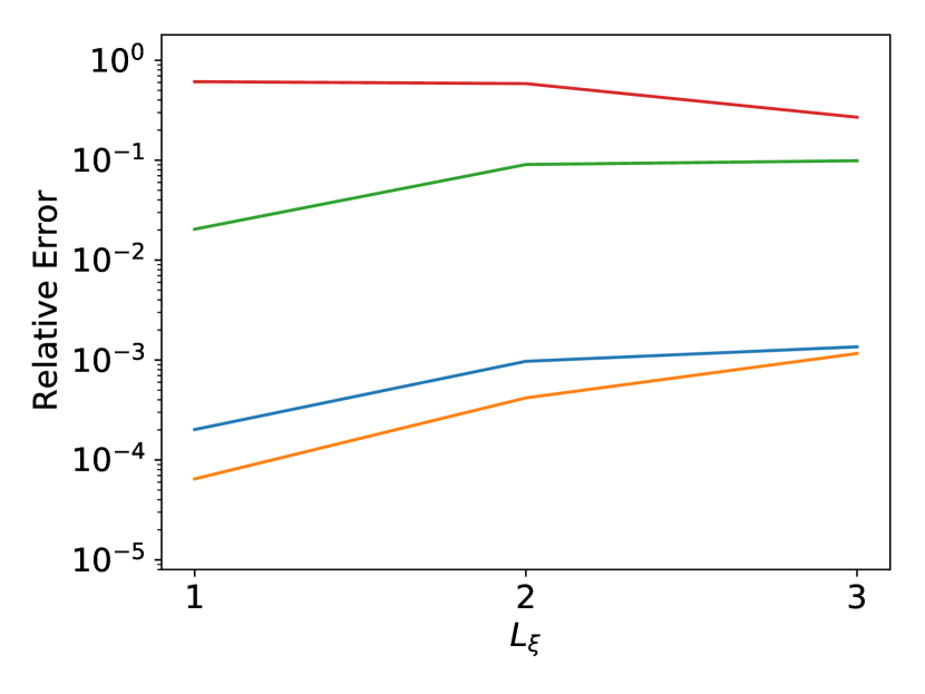
(b) DFT-Hfreq.

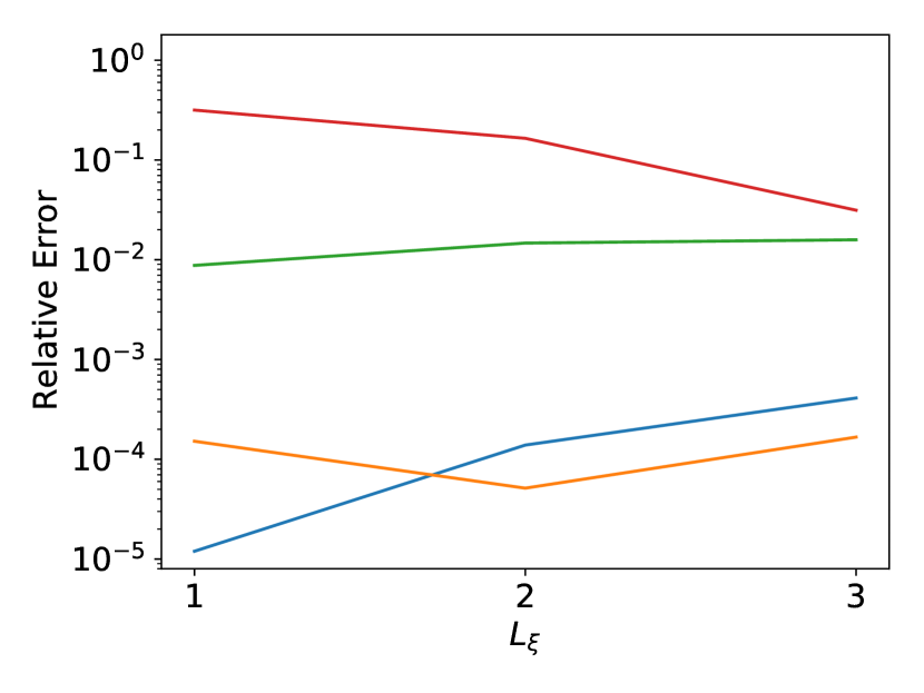
(c) DFTSmooth-Lfreq.

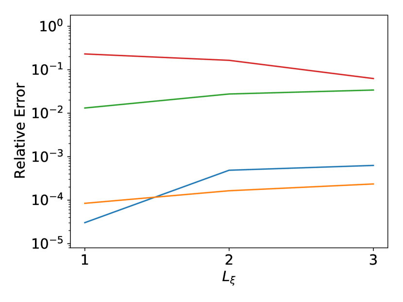
(d) DFTSmooth-Hfreq.

Figure 4: Post-training relative error against $L_{\xi}$ for all datasets. $L_{\xi}$ indicates the position of the switch layer. All four figures share the same legend as (a).

Results. Table 5 reports the result on all four datasets. Figure 4 further illustrates the post-training relative errors against $L_{\xi}$, where $L_{\xi}$ indicates the position of the switch layer. We summarize the experimental observations as follows.

1. (Weight initialization, random v.s. prefix) In all cases, training from Butterfly initialization significantly outperforms training from random initialization by two to three digits. In almost all cases, the post-training relative errors of the randomly initialized networks are not even as accurate as the pre-training relative error of the Butterfly initialized counterparts.

2. (Channel sparsity, Butterfly-net v.s. Inflated-Butterfly-net) Given a fixed $L_{\xi}$, Butterfly-net has much less parameters than Inflated-Butterfly-net. While, their post-training relative errors stay at a similar level. For these datasets, channel sparsification reduces the number of parameters without loss much post-training accuracy.

3. (Influence of datasets) Given the same input data and different output frequency windows, as in DFT-Lfreq and DFT-Hfreq, the post-training relative errors of high frequency output are slightly less accurate than their low-frequency counterparts. The impact of output frequency window on the training performance is limited. Given the same output frequency window and different input data, i.e., DFT-Lfreq v.s. DFTSmooth-Lfreq, and DFT-Hfreq v.s. DFTSmooth-Hfreq, the post-training relative errors on datasets with smoother input data are half digit to one digit more accurate than that on datasets with less smooth input data.

4. (Position of switch layer, $L_{\xi}$) The number of parameters increases as $L_{\xi}$ decreases for both Butterfly-net and Inflated-Butterfly-net. In general, the post-training relative error increases as $L_{\xi}$ increases for all Butterfly-net results. However, for Inflated-Butterfly-net with random initialization, the post-training relative error decreases as $L_{\xi}$ increases on all datasets.

We further give a discussion on the above results. The comparison of random initialization and Butterfly initialization indicates that the trainings reach two different local minima. The relative error associated with Butterfly initialization is much smaller. Numerically, we also found that if we set the learning rate for Butterfly initialized training to be large then the training loss first increases and then converges to a number worse than the results given in the Table 5. Hence, we conjecture that the energy landscape of this task is nasty and the Butterfly initialization lies in a narrow but deep well. Training from Butterfly initialization with small learning rate achieves the local minima within this narrow but deep well. Regarding the influence of datasets, the intrinsic dimensionality of the input data plays a crucial role in training. If no guidance of feature selection is provided on an intrinsically high-dimensional data, e.g., Inflated-Butterfly-net with $L_{\xi}=1$ and random initialization applied to DFT-Lfreq, the training fails to learn useful information. Adding more guidance, either refining network structure (increasing $L_{\xi}$, adding channel sparsification) or providing Butterfly initialization, helps training and achieves lower post-training relative error. However, if the intrinsic dimension of the input data is lowered, the training learns more information and achieves lower relative error. Providing extra guidance further helps training. For the position of switch layer, we can further decrease $L_{\xi}$ to zero and end up with the neural network proposed in [49]. We emphasize that when $L_{\xi}=0$, the Inflated-Butterfly-net is indeed a regular CNN. More numerical results and connections between Inflated-Butterfly-net and regular CNN refer to [49].

5.3 Comparison to CNN and Transfer Learning

This numerical experiment is to compare the Butterfly-net and Inflated-Butterfly-net on their transfer learning capability. We adopt the neural networks trained on DFTSmooth-Lfreq in previous section here. A sequence of testing datasets are generated in the same way as in previous section with $G_{\mathrm{center}}=0,2,\dots,44$ and $G_{\mathrm{width}}=10$. Each testing dataset contains 1000 samples.

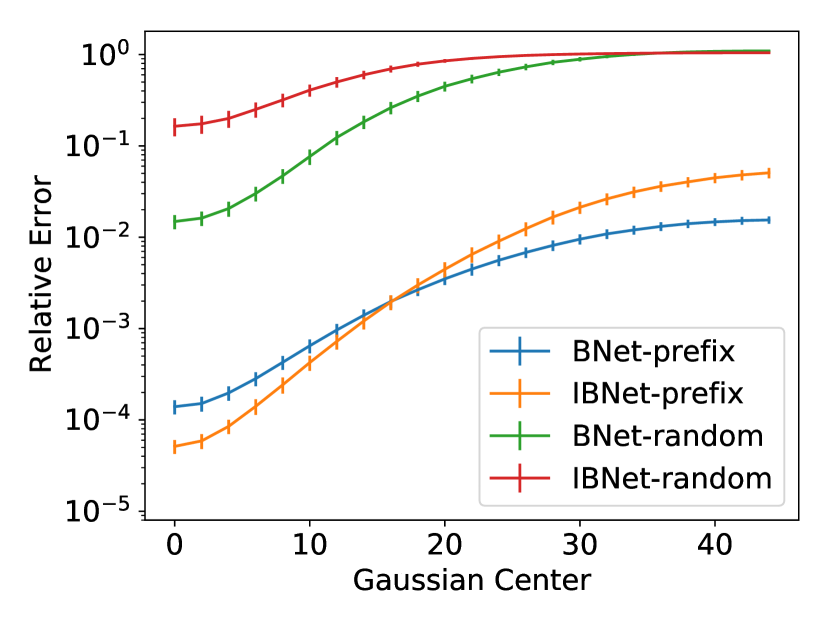
(a) $L_{\xi}=2$.

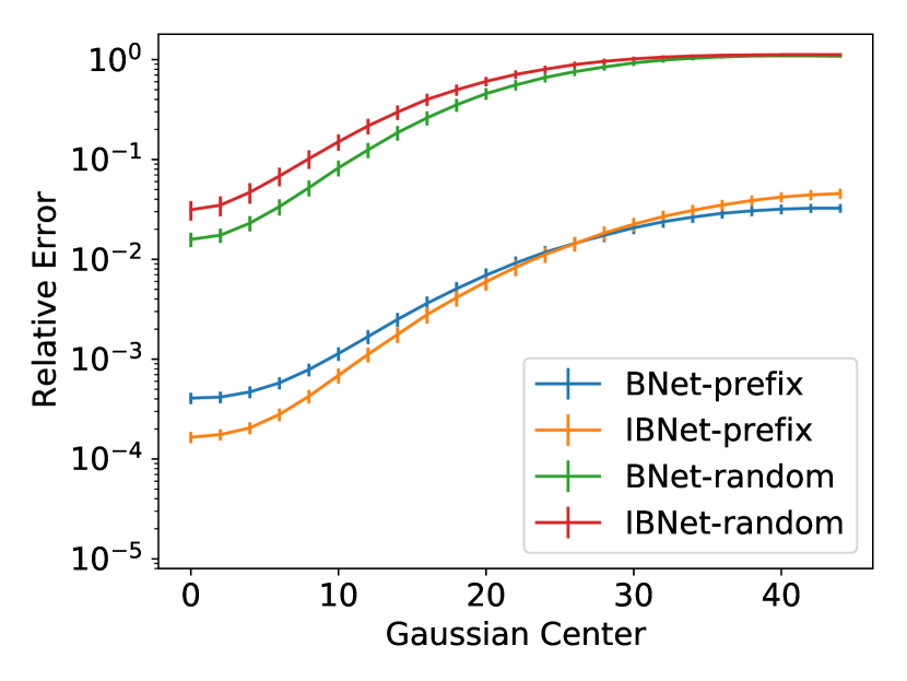
(b) $L_{\xi}=3$.

Figure 5: Mean and standard deviation for testing relative errors of Butterfly-net and Inflated-Butterfly-net on testing datasets with various $G_{\mathrm{center}}=0,2,\dots,44$ and $G_{\mathrm{width}}=10$. All networks are trained on DFTSmooth-Lfreq dataset ($G_{\mathrm{center}}=0$ and $G_{\mathrm{width}}=10$).

Figure 5 shows the means and standard deviations of the transferred testing relative errors of neural networks with $L_{\xi}=2$ and $L_{\xi}=3$. For every transferred testing, the standard deviation is orders of magnitude smaller than the corresponding mean. Hence the variation of the testing relative error for each setting is relatively small. Regarding the transfer learning capabilities, all randomly initialized networks quick loss accuracy as the testing dataset shifted away from the training dataset. While, Butterfly initialized neural networks still preserve reasonable level of accuracy. Further, comparing Butterfly-net and Inflated-Butterfly-net both with Butterfly initialization, Inflated-Butterfly-net achieves lower testing relative error when the testing dataset has significant overlap with the training dataset. However, when the overlap reduces, the testing relative error of Inflated-Butterfly-net increase faster than that of Butterfly-net. Hence we conclude that Butterfly-net has better generalizability than that of Inflated-Butterfly-net. Further, comparing the case of $L_{\xi}=2$ and $L_{\xi}=3$, we notice that the crossover of two testing relative error curves comes later in $L_{\xi}=3$. This is because that the Inflated-Butterfly-net with $L_{\xi}=3$ has much less number of parameters than that of Inflated-Butterfly-net with $L_{\xi}=2$, hence is less adapted to training dataset after training.

5.4 General Function Approximation

The last numerical example aims to construct an approximation of the energy functional of 1D Poisson’s equation and another analog functional for high frequency input data, both of which correspond directly to the approximation power in Section 4.1 in representing general functions.

Functional setup. For a Poisson’s equation $\Delta u(t)=x(t)$ with periodic boundary condition, the energy functional of Poisson’s equation is defined as the negative inner product of $u$ and $x$, which can also be approximated by a quadratic form of the leading low-frequency Fourier components,

$$\mathcal{E}_{1}(x)=-\left<x,u\right>\approx\sum_{k\in(-K,K)}\frac{1}{\absolutevalue{k}^{2}}\absolutevalue{\widehat{x}_{k}}^{2}=\sum_{k\in[1,K)}\frac{2}{\absolutevalue{k}^{2}}\absolutevalue{\widehat{x}_{k}}^{2},$$ (69)

where $\widehat{x}_{k}$ is the Fourier component of $x$ at frequency $k$ and the last equality comes from the assumption of real input $x$. If the input function $x$ is a band limited function within the frequency window, $(-K,K)$, then equality is achieved in (69). The other analogy functional for input data $x$ is defined as,

$$\mathcal{E}_{2}(x)=\sum_{k\in(K_{0},K_{0}+K)}\frac{2}{\absolutevalue{k-K_{0}}^{2}}\absolutevalue{\widehat{x}_{k}}^{2}.$$ (70)

Throughout this section, $K_{0}$ is 256 and $K$ is 128. The input data is generated in the same way as that in Section 5.2. The centers of Gaussian are $G_{\mathrm{center}}=0$ and $G_{\mathrm{center}}=256$ for $\mathcal{E}_{1}$ and $\mathcal{E}_{2}$ respectively. The widths of the Gaussian for both functionals are $G_{\mathrm{width}}=30$.

Neural network setup. Task layers are attached to Butterfly-net and Inflated-Butterfly-net. We have two different task layers, namely square-sum-layer and dense-dense-layer. The square-sum-layer first squares all output of the previous layers in Butterfly-net or Inflated-Butterfly-net, then multiplies each squared value by a weight, and finally sums them together. This is equivalent to square the output and then connect a single dense layer with one output unit. The square-sum-layer is able to exactly represent both functionals, (69) and (70) if the weights of the dense layer is properly initialized. The dense-dense-layer attaches a dense layer with 256 output units with both bias and ReLU activation function enabled. Then another dense layer with one output unit is attached afterwards. Both functionals can only be approximated by the dense-dense-layer.

Training and evaluation setup. All Butterfly-nets and Inflated-Butterfly-nets with different initializations are trained under the infinity data setting. The input data length is $N=1024$, the batch size is 256, the maximum number of iteration is $50,000$, and ADAM optimizer is used with an exponentially decay learning rate. The initial learning rate is $10^{-4}$ for Butterfly initialized networks with square-sum-layer, and is $10^{-3}$ for all other settings. The decay steps and the decay rate are 100 and 0.985 respectively. Again, the maximum number of iteration is sufficient for the convergence of relative errors in all settings. The loss function is defined as,

$$\ell(\{\vec{x}_{i}\})=\sum_{i}\absolutevalue{\mathcal{N}(\vec{x}_{i})-\mathcal{E}(\vec{x}_{i})}^{2},$$ (71)

for $\mathcal{E}$ being either $\mathcal{E}_{1}$ or $\mathcal{E}_{2}$. Relative errors are reported for comparison. The testing data is of size 1000. Default values are used for other unspecified hyper parameters.

Task Layer	$L_{\xi}$	Neural Network	Initial	Num Paras		Functional $\mathcal{E}_{1}$		Functional $\mathcal{E}_{2}$
				BNet/IBNet	Task	Pre Train	Post Train	Pre Train	Post Train
Square-sum-layer	1	BNet	prefix	136304	256	1.80$\mathrm{e-}$2	2.35$\mathrm{e-}$5	1.84$\mathrm{e-}$2	3.01$\mathrm{e-}$5
			random	136304	256	1.00$\mathrm{e-}$0	7.62$\mathrm{e-}$3	1.00$\mathrm{e-}$0	1.85$\mathrm{e-}$2
		IBNet	prefix	3533936	256	1.69$\mathrm{e-}$2	1.78$\mathrm{e-}$4	1.80$\mathrm{e-}$2	1.92$\mathrm{e-}$4
			random	3533936	256	1.00$\mathrm{e-}$0	5.80$\mathrm{e-}$3	1.00$\mathrm{e-}$0	9.48$\mathrm{e-}$3
	2	BNet	prefix	87728	256	1.79$\mathrm{e-}$2	4.36$\mathrm{e-}$5	1.72$\mathrm{e-}$2	5.84$\mathrm{e-}$5
			random	87728	256	1.00$\mathrm{e-}$0	9.62$\mathrm{e-}$3	1.00$\mathrm{e-}$0	1.74$\mathrm{e-}$2
		IBNet	prefix	915120	256	1.78$\mathrm{e-}$2	6.33$\mathrm{e-}$5	1.66$\mathrm{e-}$2	7.30$\mathrm{e-}$5
			random	915120	256	1.00$\mathrm{e-}$0	8.71$\mathrm{e-}$3	1.00$\mathrm{e-}$0	1.02$\mathrm{e-}$2
	3	BNet	prefix	66608	256	1.50$\mathrm{e-}$2	9.51$\mathrm{e-}$5	1.55$\mathrm{e-}$2	2.27$\mathrm{e-}$4
			random	66608	256	1.00$\mathrm{e-}$0	1.46$\mathrm{e-}$2	1.00$\mathrm{e-}$0	4.04$\mathrm{e-}$2
		IBNet	prefix	275504	256	1.59$\mathrm{e-}$2	5.22$\mathrm{e-}$5	1.69$\mathrm{e-}$2	1.17$\mathrm{e-}$4
			random	275504	256	1.00$\mathrm{e-}$0	1.15$\mathrm{e-}$2	1.00$\mathrm{e-}$0	2.38$\mathrm{e-}$2
Dense-dense-layer	1	BNet	prefix	136304	66048	1.00$\mathrm{e-}$0	7.44$\mathrm{e-}$3	9.99$\mathrm{e-}$1	9.30$\mathrm{e-}$3
			random	136304	66048	1.00$\mathrm{e-}$0	1.27$\mathrm{e-}$2	1.00$\mathrm{e-}$0	2.26$\mathrm{e-}$2
		IBNet	prefix	3533936	66048	9.99$\mathrm{e-}$1	4.11$\mathrm{e-}$3	1.00$\mathrm{e-}$0	5.84$\mathrm{e-}$3
			random	3533936	66048	1.00$\mathrm{e-}$0	7.67$\mathrm{e-}$3	1.00$\mathrm{e-}$0	1.44$\mathrm{e-}$2
	2	BNet	prefix	87728	66048	9.97$\mathrm{e-}$1	8.37$\mathrm{e-}$3	1.00$\mathrm{e-}$0	1.18$\mathrm{e-}$2
			random	87728	66048	1.00$\mathrm{e-}$0	2.30$\mathrm{e-}$2	1.00$\mathrm{e-}$0	2.19$\mathrm{e-}$2
		IBNet	prefix	915120	66048	1.00$\mathrm{e-}$0	5.74$\mathrm{e-}$3	9.99$\mathrm{e-}$1	7.80$\mathrm{e-}$3
			random	915120	66048	1.00$\mathrm{e-}$0	1.11$\mathrm{e-}$2	1.00$\mathrm{e-}$0	2.12$\mathrm{e-}$2
	3	BNet	prefix	66608	66048	9.99$\mathrm{e-}$1	9.83$\mathrm{e-}$3	1.00$\mathrm{e-}$0	1.01$\mathrm{e-}$2
			random	66608	66048	1.00$\mathrm{e-}$0	1.66$\mathrm{e-}$2	1.00$\mathrm{e-}$0	2.75$\mathrm{e-}$2
		IBNet	prefix	275504	66048	9.98$\mathrm{e-}$1	6.84$\mathrm{e-}$3	9.97$\mathrm{e-}$1	9.00$\mathrm{e-}$3
			random	275504	66048	1.00$\mathrm{e-}$0	1.21$\mathrm{e-}$2	1.00$\mathrm{e-}$0	3.55$\mathrm{e-}$2

Table 6: Numerical results of Butterfly-nets and Inflated-Butterfly-nets with various task layers for functional (69) and (70). Pre-training and post-training relative errors are reported for each functional. All neural networks use 16 mixing channels and $L=8$ layers.

Result. Table 6 show the results for functional (69) and (70). The comparison of the number of parameters for Butterfly-net/Inflated-Butterfly-net is the same as that in Section 5.2, while the number of parameters in dense-dense-layer is much larger than that in square-sum-layer. More accurate approximation is achieved using square-sum-layer comparing to dense-dense-layer, which is due to fact that the functionals can be exactly represented by the former task layer but not the latter. The post-training relative errors for Butterfly-net and Inflated-Butterfly-net given the same initialization, $L_{\xi}$, and task layer, remain similar in all cases. Hence the significant larger number of parameters in Inflated-Butterfly-net does not improve the post-training accuracy much. Most importantly, as we compare the post-training relative errors of different initializations under dense-dense-layer, Butterfly initialized networks achieves better accuracy comparing to its random initialized counterpart. The dense-dense-layers here are all randomly initialized and only the weights in Butterfly-net and Inflated-Butterfly-net are initialized differently. Hence we conclude that Butterfly initialization, even just on part of the whole neural network, helps finding better approximations in representing functionals (69) and (70).

6 Conclusion and Discussion

A low-complexity convolutional neural network with structured Butterfly initialization and sparse cross-channel connections is proposed, motivated by the Butterfly scheme. The functional representation by Butterfly-net is optimal in the sense that the model complexity is $O(K\log N)$ and the computational complexity is $O(N\log N)$ for $N$ and $K$ being the input and output vector lengths. The approximation accuracy to the Fourier kernel is proved to exponentially decay as the depths of the Butterfly-net increases. We also conduct an approximation analysis of Butterfly-net in representing a large class of problems in scientific computing and image and signal processing. Comparing Butterfly-net to fully connected networks, the leading term in network complexity is reduced from $\varepsilon^{-N/s}$ down to $\varepsilon^{-K/s}$, where $N$ is the input dimension, $K$ is the effective dimension, and $s$ is regularization level of the problem. Regular CNN can be viewed a special network under the analysis.

The trained Butterfly-nets from Butterfly initialization and random initialization are applied to represent discrete Fourier transforms and energy functionals. For these examples, Butterfly-net achieves better accuracy than its no-trained version. We also compared Butterfly-net against Inflated-Butterfly-net. From the numerical results, we find that Butterfly-net is able to achieve similar accuracy as Inflated-Butterfly-net, while the number of parameters is orders of magnitudes smaller. In the transfer learning settings, Butterfly-net generalizes better than Inflated-Butterfly-net when the distribution of the input data has domain shift.

The work can be extended in several directions. First, more applications of the Butterfly-net can be explored such as those in image analysis and signal processing. Likely, Butterfly-net is able to replace some CNN structures in practice such that similar accuracy can be achieved while the parameter number is much reduced. Second, our current theoretical analysis does not address the case when the input data contain noise. In particular, adding rectified layers in Butterfly-net can be interpreted as a thresholding denoising operation applied to the intermediate representations; a statistical analysis is desired.

Acknowledgments

The work of YL and JL is supported in part by National Science Foundation via grants DMS-1454939 and ACI-1450280. XC is partially supported by NSF (DMS-1818945, DMS-1820827), NIH (grant R01GM131642) and the Alfred P. Sloan Foundation.

Appendix A Proof of Theorem 2.1

Here we first include a well-known lemma of Chebyshev interpolation for completeness and then prove Theorem 2.1.

Lemma A.1.

Let $f(y)\in C_{[a,b]}$ and $\mathcal{P}_{r}$ be the space spanned by the monomials $y^{r}$. The projection operator $\Pi_{r}$ mapping $f$ into its Lagrange interpolation on the $r$ Chebyshev grid obeys,

$$\norm{f-\Pi_{r}f}_{\infty}\leq\left(2+\frac{2}{\pi}\ln r\right)\inf_{g\in\mathcal{P}_{r}}\norm{f-g}_{\infty}.$$ (72)

The proof of Lemma A.1 can be found in [45].

Proof of Theorem 2.1.

The Fourier kernel $\mathcal{K}\left(\xi,t\right)=e^{-2\pi\imath\xi\cdot t}$ can be decomposed as,

$$\begin{split}\mathcal{K}\left(\xi,t\right)&=e^{-2\pi\imath\left(\xi\cdot t-\xi_{0}\cdot t-\xi\cdot t_{0}+\xi_{0}\cdot t_{0}\right)}\cdot e^{-2\pi\imath\xi_{0}\cdot t}\cdot e^{-2\pi\imath\xi\cdot t_{0}}\cdot e^{2\pi\imath\xi_{0}\cdot t_{0}}\\ &=e^{-2\pi\imath R(\xi,t)}\cdot e^{-2\pi\imath\xi_{0}\cdot t}\cdot e^{-2\pi\imath\xi\cdot t_{0}}\cdot e^{2\pi\imath\xi_{0}\cdot t_{0}},\end{split}$$ (73)

where $R(\xi,t)=\left(\xi-\xi_{0}\right)\cdot\left(t-t_{0}\right)$, $t_{0}$ and $\xi_{0}$ are centers of $B$ and $A$ respectively.

Next, we show the $r$-term truncation error for the first term in the second line of (73). Based on the power expansion of $e^{-2\pi\imath R(\xi,t)}$, i.e.,

$$e^{-2\pi\imath R(\xi,t)}=\sum_{k=0}^{\infty}\frac{\left(-2\pi\imath R(\xi,t)\right)^{k}}{k!},$$ (74)

the $r$-term truncation error can be bounded as,

$$\begin{split}\delta&=\absolutevalue{e^{-2\pi\imath R(\xi,t)}-\sum_{k=0}^{r}\frac{\left(-2\pi\imath R(\xi,t)\right)^{k})}{k!}}=\absolutevalue{\sum_{k=r+1}^{\infty}\frac{\left(-2\pi\imath R(\xi,t)\right)^{k}}{k!}}\\ &\leq\sum_{k=r+1}^{\infty}\frac{(\pi w(A)w(B))^{k}}{2^{k}k!}\leq\sum_{k=r+1}^{\infty}\left(\frac{\pi ew(A)w(B)}{2k}\right)^{k}\leq\left(\frac{\pi ew(A)w(B)}{2r}\right)^{r},\end{split}$$ (75)

where the last inequality uses $w(A)w(B)\leq\frac{r}{\pi e}$. We also notice that, for any fixed $\xi$, $\sum_{k=0}^{r}\frac{\left(2\pi\imath R(\xi,\cdot)\right)^{k}}{k!}\in\mathcal{P}_{r}$. Applying Lemma A.1, we obtain,

$$\norm{e^{-2\pi\imath R(\xi,t)}-\sum_{k=1}^{r}e^{-2\pi\imath R(\xi,t_{k})}\mathcal{L}_{k}(t)}_{\infty}\leq\left(2+\frac{2}{\pi}\ln r\right)\delta.$$ (76)

By substituting the explicit expression of $R(\xi,t)$, we obtain one of the conclusion,

$$\norm{e^{-2\pi\imath\xi\cdot t}-\sum_{k=1}^{r}e^{-2\pi\imath\xi\cdot t_{k}}e^{-2\pi\imath\xi_{0}\cdot\left(t-t_{k}\right)}\mathcal{L}_{k}(t)}_{\infty}\leq\left(2+\frac{2}{\pi}\ln r\right)\left(\frac{\pi ew(A)w(B)}{2r}\right)^{r},$$ (77)

for any $\xi\in A$ and $t\in B$.

Similarly, for any fixed $t$, we have $\sum_{k=0}^{r}\frac{\left(2\pi\imath R(\xi,t)\right)^{k}}{k!}\in\mathcal{P}_{r}(\xi)$. Hence the second conclusion can be obtained through the same procedure. ∎

Appendix B Complex valued operation with ReLU activation function

A complex-valued linear operator can be represented through real-valued operation with ReLU activation function. Assume we want to represent the complex-valued linear operation,

$$y=ax$$ (78)

where $x,y\in\mathbb{C}$ can be generalized to vectors and $a\in\mathbb{C}$ can be generalized to a complex-valued matrix. We first introduce the real-valued representation for complex numbers/vectors. A complex number $x=\real x+\imath\imaginary x\in\mathbb{C}$ is represented as

$$\begin{pmatrix}(\real x)_{+}&(\imaginary x)_{+}&(\real x)_{-}&(\imaginary x)_{-}\end{pmatrix}^{\top},$$ (79)

where $(z)_{+}=\max(z,0)$ and $(z)_{-}=-\min(z,0)$ for any $z\in\mathbb{R}$. If $x$ is a complex vector of size $n$, then the real-valued representation concatenates (79) for each complex value and results a real vector of size $4n$.

The multiplication $y=ax$ is produced as the ReLU activation function acting on a matrix vector multiplication, i.e.,

$$\sigma\left(\begin{pmatrix}\real a&-\imaginary a&-\real a&\imaginary a\\ \imaginary a&\real a&-\imaginary a&-\real a\\ -\real a&\imaginary a&\real a&-\imaginary a\\ -\imaginary a&-\real a&\imaginary a&\real a\\ \end{pmatrix}\begin{pmatrix}(\real x)_{+}\\ (\imaginary x)_{+}\\ (\real x)_{-}\\ (\imaginary x)_{-}\end{pmatrix}\right)=\begin{pmatrix}(\real y)_{+}\\ (\imaginary y)_{+}\\ (\real y)_{-}\\ (\imaginary y)_{-}\end{pmatrix},$$ (80)

where the complex-valued linear operator $a$ is extended to be a real-valued $4\times 4$ matrix. Extension of $a$ to a matrix can also be done through concatenating in both row and column directions.

In order to simplify the description in this paper, we define an extensive assign operator as $\overset{\diamond}{=}$ such that the 4 by 4 matrix $A$ in (80) then obeys $A\overset{\diamond}{=}a$.

The above description can also be found in [49].

Appendix C Example signals of datasets

We provide instance input and output data for each dataset in Table 4, namely Figure 6 for DFT-Lfreq, Figure 7 for DFT-Hfreq, Figure 8 for DFTSmooth-Lfreq, and Figure 9 for DFTSmooth-Hfreq.

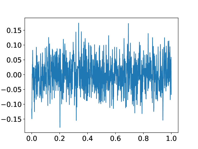
(a) Input data $\vec{x}$.

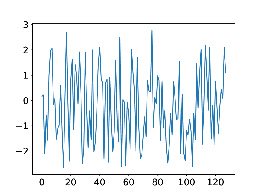
(b) Real part of output data $\vec{y}$.

Figure 6: One instance in dataset DFT-Lfreq.

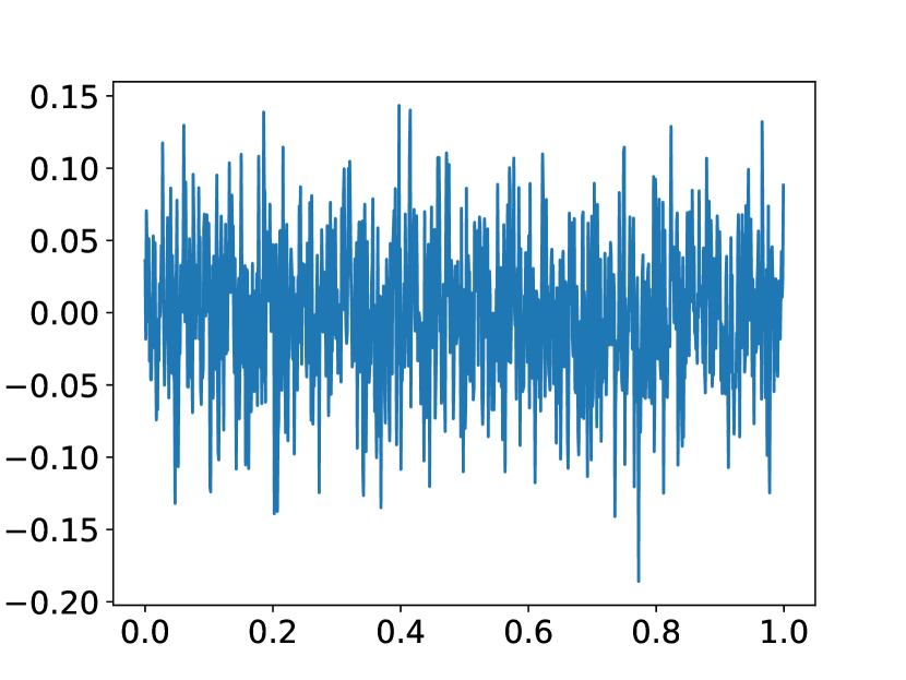
(a) Input data $\vec{x}$.

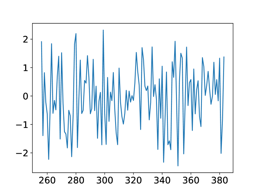
(b) Real part of output data $\vec{y}$.

Figure 7: One instance in dataset DFT-Hfreq.

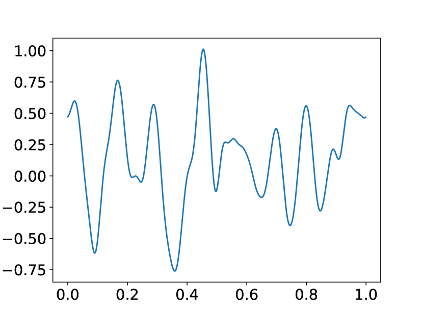
(a) Input data $\vec{x}$.

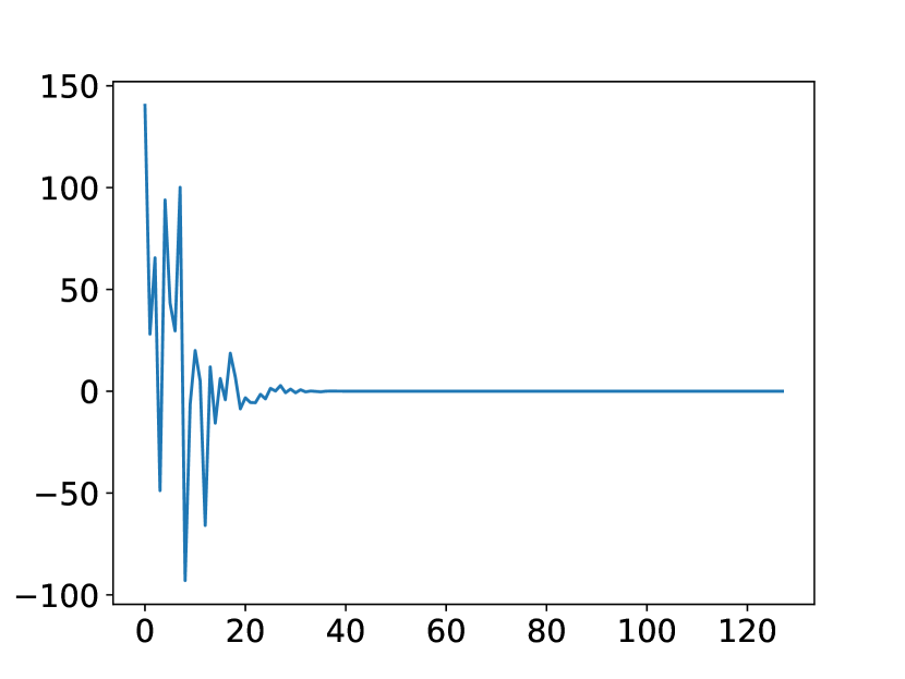
(b) Real part of output data $\vec{y}$.

Figure 8: One instance in dataset DFTSmooth-Lfreq.

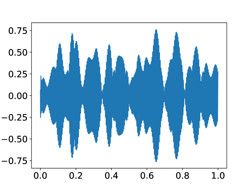
(a) Input data $\vec{x}$.

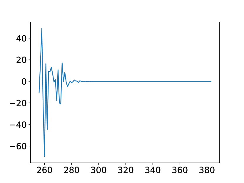
(b) Real part of output data $\vec{y}$.

Figure 9: One instance in dataset DFTSmooth-Hfreq.

Appendix D Convergence behaviors

We provide four convergence behaviors for the training loss of Butterfly-net and Inflated-Butterfly-net with random and Butterfly initialization applied to DFTSmooth-Lfreq in Figure 10. In all four networks, the number of layers after switch layer is $L_{\xi}=1$. Other settings have the similar convergence behaviors.

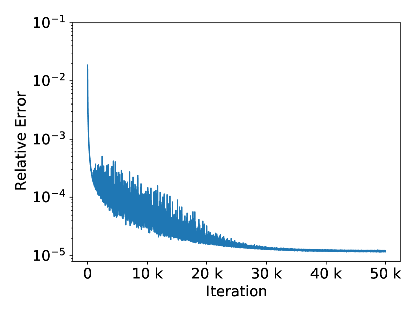
(a) Butterfly-net with Butterfly initialization.

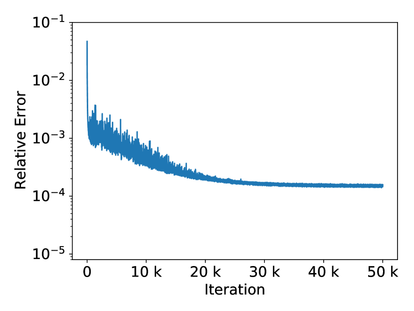
(b) Inflated-Butterfly-net with Butterfly initialization.

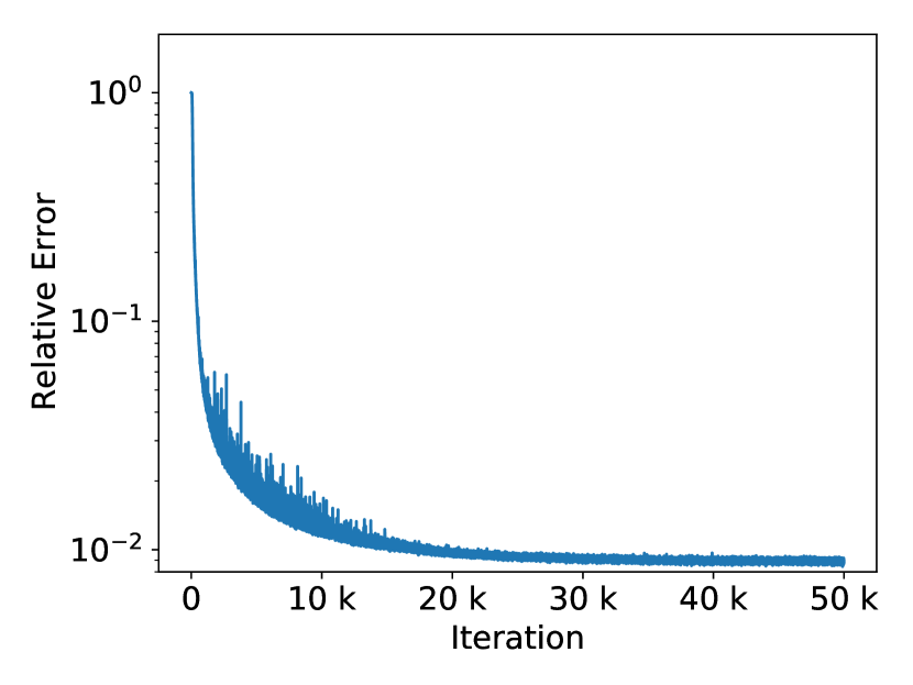
(c) Butterfly-net with random initialization.

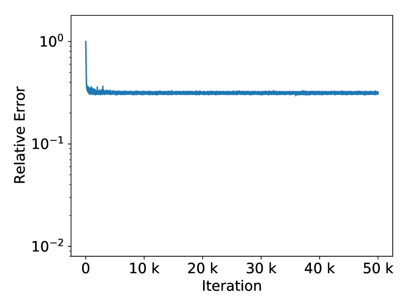
(d) Inflated-Butterfly-net with random initialization.

Figure 10: Convergence behavior for various networks applied to DFTSmooth-Lfreq dataset. The number of layers after switch layer for all networks is $L_{\xi}=1$.

References

- Abadi et al. [2015] Martín Abadi, Ashish Agarwal, Paul Barham, Eugene Brevdo, Zhifeng Chen, Craig Citro, Greg S. Corrado, Andy Davis, Jeffrey Dean, Matthieu Devin, Sanjay Ghemawat, Ian Goodfellow, Andrew Harp, Geoffrey Irving, Michael Isard, Yangqing Jia, Rafal Jozefowicz, Lukasz Kaiser, Manjunath Kudlur, Josh Levenberg, Dandelion Mané, Rajat Monga, Sherry Moore, Derek Murray, Chris Olah, Mike Schuster, Jonathon Shlens, Benoit Steiner, Ilya Sutskever, Kunal Talwar, Paul Tucker, Vincent Vanhoucke, Vijay Vasudevan, Fernanda Viégas, Oriol Vinyals, Pete Warden, Martin Wattenberg, Martin Wicke, Yuan Yu, and Xiaoqiang Zheng. TensorFlow: Large-scale machine learning on heterogeneous systems, 2015. URL https://www.tensorflow.org/. Software available from tensorflow.org.
- Bao et al. [2019] Chenglong Bao, Qianxiao Li, Zuowei Shen, Cheng Tai, Lei Wu, and Xueshuang Xiang. Approximation analysis of convolutional neural networks, 2019.
- Barron [1993] Andrew R Barron. Universal approximation bounds for superpositions of a sigmoidal function. IEEE Transactions on Information theory, 39(3):930–945, 1993.
- Behler and Parrinello [2007] Jörg Behler and Michele Parrinello. Generalized neural-network representation of high-dimensional potential-energy surfaces. Physical review letters, 98(14):146401, 2007.
- Bengio et al. [2015] Yoshua Bengio, Ian J Goodfellow, and Aaron Courville. Deep learning. Nature, 521(7553):436–444, 2015.
- Berg and Nyström [2018] Jens Berg and Kaj Nyström. A unified deep artificial neural network approach to partial differential equations in complex geometries. Neurocomputing, 317:28 – 41, 2018. ISSN 0925-2312. doi: https://doi.org/10.1016/j.neucom.2018.06.056. URL http://www.sciencedirect.com/science/article/pii/S092523121830794X.
- Bölcskei et al. [2019] H. Bölcskei, P. Grohs, G. Kutyniok, and P. Petersen. Optimal approximation with sparsely connected deep neural networks. SIAM Journal on Mathematics of Data Science, 1(1):8–45, 2019. doi: 10.1137/18M118709X. URL https://doi.org/10.1137/18M118709X.
- Cai et al. [2012] Jian-Feng Cai, Bin Dong, Stanley Osher, and Zuowei Shen. Image restoration: total variation, wavelet frames, and beyond. Journal of the American Mathematical Society, 25(4):1033–1089, 2012.
- Candès et al. [2007] Emmanuel J. Candès, Laurent Demanet, and Lexing Ying. Fast computation of Fourier integral operators. SIAM J. Sci. Comput., 29(6):2464–2493, jan 2007. URL http://epubs.siam.org/doi/abs/10.1137/060671139.
- Candès et al. [2009] Emmanuel J. Candès, Laurent Demanet, and Lexing Ying. A fast butterfly algorithm for the computation of Fourier integral operators. Multiscale Model. Simul., 7(4):1727–1750, jan 2009. URL http://epubs.siam.org/doi/abs/10.1137/080734339.
- Chan and Shen [2005] Tony F Chan and Jianhong Jackie Shen. Image processing and analysis: variational, PDE, wavelet, and stochastic methods, volume 94. SIAM, 2005.
- Cohen et al. [2016] Nadav Cohen, Or Sharir, and Amnon Shashua. On the expressive power of deep learning: A tensor analysis. In Conference on Learning Theory, pages 698–728, 2016.
- Cybenko [1989] George Cybenko. Approximation by superpositions of a sigmoidal function. Mathematics of control, signals and systems, 2(4):303–314, 1989.
- Delalleau and Bengio [2011] Olivier Delalleau and Yoshua Bengio. Shallow vs. deep sum-product networks. In Advances in Neural Information Processing Systems, pages 666–674, 2011.
- Demanet and Ying [2011] Laurent Demanet and Lexing Ying. Discrete symbol calculus. SIAM Rev., 53(1):71–104, jan 2011. URL http://epubs.siam.org/doi/10.1137/080731311.
- Demanet et al. [2012] Laurent Demanet, Matthew Ferrara, Nicholas Maxwell, Jack Poulson, and Lexing Ying. A butterfly algorithm for synthetic aperture radar imaging. SIAM Journal on Imaging Sciences, 5(1):203–243, jan 2012. URL http://epubs.siam.org/doi/10.1137/100811593.
- E et al. [2017] Weinan E, Jiequn Han, and Arnulf Jentzen. Deep learning-based numerical methods for high-dimensional parabolic partial differential equations and backward stochastic differential equations. Communications in Mathematics and Statistics, 5(4):349–380, 2017.
- Eldan and Shamir [2016] Ronen Eldan and Ohad Shamir. The power of depth for feedforward neural networks. In Conference on Learning Theory, pages 907–940, 2016.
- Fan and Ying [2019] Yuwei Fan and Lexing Ying. Solving electrical impedance tomography with deep learning, jun 2019. http://arxiv.org/abs/1906.03944.
- Fan et al. [2018] Yuwei Fan, Lin Lin, Lexing Ying, and Leonardo Zepeda-Núñez. A multiscale neural network based on hierarchical matrices, 2018. https://arxiv.org/abs/1807.01883.
- Fan et al. [2019a] Yuwei Fan, Jordi Feliu-Fabà, Lin Lin, Lexing Ying, and Leonardo Zepeda-Núñez. A multiscale neural network based on hierarchical nested bases. Res. Math. Sci., 6(2):21, mar 2019a. doi: 10.1007/s40687-019-0183-3.
- Fan et al. [2019b] Yuwei Fan, Cindy Orozco Bohorquez, and Lexing Ying. BCR-Net: A neural network based on the nonstandard wavelet form. J. Comput. Phys., 384:1–15, may 2019b. doi: 10.1016/J.JCP.2019.02.002.
- Feliu-Faba et al. [2019] Jordi Feliu-Faba, Yuwei Fan, and Lexing Ying. Meta-learning pseudo-differential operators with deep neural networks, jun 2019. http://arxiv.org/abs/1906.06782.
- Gallant and White [1988] A Ronald Gallant and Halbert White. There exists a neural network that does not make avoidable mistakes. In Proceedings of the Second Annual IEEE Conference on Neural Networks, San Diego, CA, I, 1988.
- He and Xu [2019] Juncai He and Jinchao Xu. MgNet: A unified framework of multigrid and convolutional neural network. Science China Mathematics, 62(7):1331–1354, jul 2019. doi: 10.1007/s11425-019-9547-2. URL http://link.springer.com/10.1007/s11425-019-9547-2.
- Hornik et al. [1989] Kurt Hornik, Maxwell Stinchcombe, and Halbert White. Multilayer feedforward networks are universal approximators. Neural networks, 2(5):359–366, 1989.
- Khoo and Ying [2018] Yuehaw Khoo and Lexing Ying. SwitchNet: a neural network model for forward and inverse scattering problems, oct 2018. http://arxiv.org/abs/1810.09675.
- Khoo et al. [2018] Yuehaw Khoo, Jianfeng Lu, and Lexing Ying. Solving for high-dimensional committor functions using artificial neural networks. Research in the Mathematical Sciences, 6(1):1, 2018. ISSN 2197-9847. doi: 10.1007/s40687-018-0160-2. URL https://doi.org/10.1007/s40687-018-0160-2.
- Kunis and Melzer [2012] Stefan Kunis and Ines Melzer. A stable and accurate butterfly sparse Fourier transform. SIAM J. Numer. Anal., 50(3):1777–1800, jan 2012. URL http://epubs.siam.org/doi/10.1137/110839825.
- Le Roux and Bengio [2008] Nicolas Le Roux and Yoshua Bengio. Representational power of restricted Boltzmann machines and deep belief networks. Neural computation, 20(6):1631–1649, 2008.
- Li and Yang [2017] Yingzhou Li and Haizhao Yang. Interpolative butterfly factorization. SIAM J. Sci. Comput., 39(2):A503–A531, 2017. URL http://dx.doi.org/10.1137/16M1074941.
- Li et al. [2015a] Yingzhou Li, Haizhao Yang, Eileen R. Martin, Kenneth L. Ho, and Lexing Ying. Butterfly factorization. Multiscale Model. Simul., 13(2):714–732, jan 2015a. URL http://epubs.siam.org/doi/10.1137/15M1007173.
- Li et al. [2015b] Yingzhou Li, Haizhao Yang, and Lexing Ying. A multiscale butterfly algorithm for multidimensional Fourier integral operators. Multiscale Model. Simul., 13(2):1–18, jan 2015b. URL http://epubs.siam.org/doi/10.1137/140997658http://arxiv.org/abs/1411.7418.
- Li et al. [2018] Yingzhou Li, Haizhao Yang, and Lexing Ying. Multidimensional butterfly factorization. Applied and Computational Harmonic Analysis, 44(3):737–758, may 2018. doi: 10.1016/J.ACHA.2017.04.002. URL https://www.sciencedirect.com/science/article/pii/S1063520317300271.
- Li et al. [2019] Yingzhou Li, Jianfeng Lu, and Anqi Mao. Variational training of neural network approximations of solution maps for physical models, may 2019. http://arxiv.org/abs/1905.02789.
- Liang and Srikant [2016] Shiyu Liang and R Srikant. Why deep neural networks for function approximation? arXiv preprint arXiv:1610.04161, 2016.
- Long et al. [2018] Zichao Long, Yiping Lu, Xianzhong Ma, and Bin Dong. PDE-net: Learning PDEs from data. 80:3208–3216, 2018. URL http://proceedings.mlr.press/v80/long18a.html.
- Lu et al. [2020] Jianfeng Lu, Zuowei Shen, Haizhao Yang, and Shijun Zhang. Deep network approximation for smooth functions, jan 2020. http://arxiv.org/abs/2001.03040.
- Mallat [2008] Stephane Mallat. A wavelet tour of signal processing: the sparse way. Academic press, 2008.
- Mhaskar et al. [2016] Hrushikesh Mhaskar, Qianli Liao, and Tomaso Poggio. Learning functions: when is deep better than shallow. arXiv preprint arXiv:1603.00988, 2016.
- Mhaskar and Poggio [2016] Hrushikesh N Mhaskar and Tomaso Poggio. Deep vs. shallow networks: An approximation theory perspective. Analysis and Applications, 14(06):829–848, 2016.
- Michielssen and Boag [1996] Eric Michielssen and Amir Boag. A multilevel matrix decomposition algorithm for analyzing scattering from large structures. IEEE Trans. Antennas Propag., 44(8):1086–1093, 1996. URL http://ieeexplore.ieee.org/document/511816/.
- Montufar et al. [2014] Guido F Montufar, Razvan Pascanu, Kyunghyun Cho, and Yoshua Bengio. On the number of linear regions of deep neural networks. In Advances in neural information processing systems, pages 2924–2932, 2014.
- O’Neil et al. [2010] Michael O’Neil, Franco Woolfe, and Vladimir Rokhlin. An algorithm for the rapid evaluation of special function transforms. Appl. Comput. Harmon. Anal., 28(2):203–226, 2010.
- Rivlin [1990] Theodore J. Rivlin. Chebyshev polynomials: from approximation theory to algebra and number theory. Wiley-Interscience, 2nd edition, 1990.
- Ronneberger et al. [2015] Olaf Ronneberger, Philipp Fischer, and Thomas Brox. U-net: Convolutional networks for biomedical image segmentation. In Med. Image Comput. Comput. Interv., volume 9351, pages 234–241. Springer Verlag, 2015. ISBN 9783319245737. doi: 10.1007/978-3-319-24574-4_28.
- Schneider et al. [2017] Elia Schneider, Luke Dai, Robert Q Topper, Christof Drechsel-Grau, and Mark E Tuckerman. Stochastic neural network approach for learning high-dimensional free energy surfaces. Physical review letters, 119(15):150601, 2017.
- Telgarsky [2016] Matus Telgarsky. Benefits of depth in neural networks. 49:1517–1539, 2016. URL http://proceedings.mlr.press/v49/telgarsky16.html.
- Xu et al. [2019] Zhongshu Xu, Yingzhou Li, and Xiuyuan Cheng. Butterfly-Net2: Simplified butterfly-net and Fourier transform initialization, dec 2019. http://arxiv.org/abs/1912.04154.
- Yarotsky [2017a] Dmitry Yarotsky. Error bounds for approximations with deep ReLU networks. Neural Networks, 94:103–114, oct 2017a. ISSN 18792782. doi: 10.1016/j.neunet.2017.07.002.
- Yarotsky [2017b] Dmitry Yarotsky. Error bounds for approximations with deep ReLU networks. Neural Networks, 94:103–114, 2017b.
- Ying [2009] Lexing Ying. Sparse Fourier transform via butterfly algorithm. SIAM J. Sci. Comput., 31(3):1678–1694, jan 2009. URL http://epubs.siam.org/doi/10.1137/08071291X.
- Zhang et al. [2018] Linfeng Zhang, Jiequn Han, Han Wang, Roberto Car, and Weinan E. Deepcg: Constructing coarse-grained models via deep neural networks. The Journal of Chemical Physics, 149(3):034101, 2018. doi: 10.1063/1.5027645. URL https://doi.org/10.1063/1.5027645.
- Zhou [2019] Ding-Xuan Zhou. Universality of deep convolutional neural networks. Applied and Computational Harmonic Analysis, 2019. ISSN 1063-5203. doi: https://doi.org/10.1016/j.acha.2019.06.004. URL http://www.sciencedirect.com/science/article/pii/S1063520318302045.