Efficient Atlasing and Search of Configuration Spaces of Point-Sets Constrained by Distance Intervals.

Abstract

For configurations of point-sets that are pairwise constrained by distance intervals, the EASAL software implements a suite of algorithms that characterize the structure and geometric properties of the configuration space. The algorithms generate, describe and explore these configuration spaces using generic rigidity properties, classical results for stratification of semi-algebraic sets, and new results for efficient sampling by convex parametrization. The paper reviews the key theoretical underpinnings, major algorithms and their implementation. The paper outlines the main applications such as the computation of free energy and kinetics of assembly of supramolecular structures or of clusters in colloidal and soft materials. In addition, the paper surveys select experimental results and comparisons.

1 Introduction

We present a software implementation of the algorithm EASAL (Efficient Atlasing and Search of Assembly Landscapes) [44]. This implementation generates, describes, and explores the feasible relative positions of two point-sets $A$ and $B$ of size $n$ in $\mathbb{R}^{3}$ that are mutually constrained by distance intervals. Formally, a Euclidean orientation-preserving isometry $T\in SE(3)$ is feasible if, for $\emph{dist}_{a,b}$ defined as the Euclidean norm $||a-T(b)||$, the following hold:

$$\forall(a\in A,b\in B),\qquad \emph{dist}_{a,b}\qquad\geq\rho_{a,b} C_{1}$$ ()

$$\exists(a\in A,b\in B),\qquad \emph{dist}_{a,b}-\rho_{a,b}\leq\delta_{a,b}, \rho_{a,b},\delta_{a,b}\in\mathbb{R}_{+}. C_{2}$$ ()

Constraint $C_{1}$ means that $T$ is infeasible when there exists a pair $(a,T(b))$ that is too close. Constraint $C_{2}$ implies that at least one pair $(a,T(b))$ is within a preferred distance interval. Consider for example, sets $A$ and $B$ of centers of non-intersecting spheres (see Fig. 2(a) and Fig. 3(a)). With $\rho_{a}$, $\rho_{b}$ the sphere radii, the constant $\rho_{a,b}$ in $C_{1}$ equals $\rho_{a}+\rho_{b}$. Note that the ambient dimension of Problem ($C_{1}$, $C_{2}$) is 6, namely, the dimension of SE(3). When $T$ is feasible, the Cartesian configuration $T(B)$ is called a realization of the constraint system ($C_{1}$, $C_{2}$). When $\delta_{a,b}\approx 0$ the effective dimension of the realization space is 5.

The input to EASAL consists of up to four components.

1. $k=2$ point-sets $A$ and $B$ with $n$ points each. (The submitted implementation is for two point-sets, but the theory and the algorithms generalize to $k$ point-sets and ambient dimension $6(k-1)$)

2. The pairwise distance interval parameters $\rho_{a,b},\delta_{a,b}\in\mathbb{R}_{+}$.

3. Optional: global constraints imposed on the overall configuration.

4. Optional: a set of active constraints of interest. (Only constraint regions including at least one of these active constraints is sampled and added to the atlas.)

The main output of EASAL is the dimensional, topological and geometric structure of the realization space, i.e., all $T(B)$ satisfying ($C_{1}$, $C_{2}$). The realization space is represented as the sweep of the individual realizations (see Fig. 2(d) and Fig. 3(b)). The sweep representation shows $A$ together with all feasible realizations $T(B)$ traced out.

To describe this space, EASAL employs three strategies. First, EASAL partitions the realization space into active constraint regions, each defined by the set of active constraints, i.e., the pairs $(a,b)$ satisfying $C_{2}$. These pairs are edges of the active constraint graph used to label the region. Such a graph can be analyzed by generic combinatorial rigidity theory [19], in particular, the co-dimension of an active constraint region (see Section 2.1) is typically the number of active constraint edges. Since the active constraint regions satisfy polynomial equations and inequalities, the realization space is semi-algebraic set (a union of sets defined by polynomial inequalities). This is the setting of a Thom-Whitney stratification of semi-algebraic sets [38].

Second, EASAL organizes and represents the active constraint regions in a partial order (directed acyclic graph) so that the active constraint graph of a region is a subgraph of the active constraint graph of its boundary regions. This organization is called the atlas. To construct the atlas, EASAL recursively starts from the interior of an active constraint region and locates boundary regions of strictly one dimension less. Such boundary regions generically have exactly one additional active constraint and the active constraint graph has one additional edge. Considering only boundary regions of exactly one dimension less improves robustness over searching directly for lowest-dimensional regions. We note that, when a new child region of one dimension less is found, all its higher dimensional ancestor regions are immediately discovered since they correspond to a subset of the active constraints. Therefore, even if a region is missed at some stage, it will be discovered once any of its descendants are found, for example, through one of its siblings.

Third, to locate the boundary region satisfying an additional active constraint, EASAL applies the theoretical framework developed in [52]. EASAL efficiently maps (many to one) a $d$-dimensional active constraint region $R$ with active constraint graph $G$, to a convex region of $\mathbb{R}^{d}$ called the Cayley configuration space of $R$. Define a non-edge of $G$ as a pair $(a,b)$ not connected by an edge in $G$. The Cayley configuration space of $R$ is defined intuitively as the set of realizable lengths of $d$ chosen non-edges of $G$. The variables representing these non-edge lengths are called the Cayley parameters. In what follows, we simply refer to the non-edges as Cayley parameters. Since the Cayley configuration space is convex, it allows for efficient sampling and search. In addition, it is efficient to compute the inverse map from each point in the Cayley configuration space (a Cayley configuration) to its finitely many corresponding Cartesian realizations. The Cayley configuration space of a $d$-dimensional active constraint region $R$ is discretized and represented as a $d$-dimensional grid. The Cayley points adjacent to the lower dimensional boundary regions of $R$ are highlighted in different colors (See Fig. 2(b)).

Efficiency, accuracy, and tradeoff guarantees have been formally established for EASAL (see Section 3.5). The total number of active constraint regions in the atlas could be as large as $O(k^{2}\cdot n^{12k})$. The maximum dimension of a region is $6(k-1)$. If $r$ regions of dimension $d$ have to be sampled, EASAL requires time linear in $r$ and exponential in $d$. EASAL can explore assemblies up to a million regions for small assemblies in a few hours on a standard laptop (see Section 4.1). By small assemblies we mean constraint problems with $n\leq 5000$ and $k=2$; or $n\leq 3$ and $k\leq 18$. Efficiency can improve significantly when the point-sets are identical, by exploiting symmetries in the configuration space [54].

Section 4 surveys numerical experimental results from [53], for (i) generating the atlas, (ii) using the atlas to find paths between active constraint regions and (iii) using the atlas to find the neighbor regions of an active constraint region. We also survey experimental results from [42], comparing the performance of EASAL with Metropolis Markov chain Monte Carlo (MC) and from [60] for EASAL predicting the sensitivity of icosahedral T=1 viruses towards assembly disruption.

Organization: After briefly reviewing applications of EASAL to molecular and materials modeling and related work, the remainder of the paper is organized as follows. Section 2 discusses the theory underlying EASAL. Section 3 discusses the algorithmic ideas and implementation. Section 4 surveys experimental results, Section 5 sketches the software architecture.

1.1 Application to Molecular and Materials Modeling

EASAL provides a new approach to the longstanding challenges in molecular and soft-matter self-assembly under short range potential interactions. EASAL can be used to estimate free-energy, binding affinity and kinetics. For example, EASAL can be applied to (a) supramolecular self-assembly or docking starting from rigid molecular motifs e.g., helices, peptides, ligands etc. or (b) self-assembly of clusters of multiple particles each consisting of 1-3 spheres - e.g., in amphiphiles, colloids or liquid crystals.

In the context of molecular assembly, rigid components of the molecules correspond to the input point-sets $A$ and $B$, and atoms correspond to the points $a\in A$ and $b\in B$. The active constraint regions correspond to regions of constant potential energy derived from discretized Lennard-Jones [28] potential energy terms. It is intractable or at least prodigiously expensive to atlas large molecular assemblies by any naive global method. Assemblies are typically recursively decomposed into smaller assemblies (defined above) and recombined. Generally, the input molecules have a small set of interfaces (pairs of atoms, one from each molecule) where bond formation is feasible. These are given as input by specifying a set of active constraints of interest corresponding to the interfaces. EASAL atlases only those $r$ active constraint regions where at least one of these constraints is active (i.e., $C_{2}$ holds).

1.1.1 Geometrization of Molecular Interactions in EASAL

In EASAL, the inter-atomic Lennard-Jones potential energy terms are geometrized into 3 main regions: (i) large distances at which no force is exerted between the atoms, such atom pairs, called inactive constraints, correspond to $(a,b)$ such that $dist_{a,b}>\rho_{a,b}+\delta_{a,b}$, (ii) very close distances that are prohibited by inter-atomic repulsion or inter-atomic collisions and violating $C_{1}$. (iii) the interval between these, known as the Lennard-Jones well, in which bonds are formed, corresponding to the preferred distance or active constraints defined in $C_{2}$.

The pairwise Lennard-Jones terms are typically input only for selected pairs of atoms, one from each rigid component. Hard-sphere steric constraints, apply to all other pairs and enforce (i) and (ii) with $\delta_{a,b}=0$ in $C_{2}$. Having more active constraints corresponds to lower potential energy, as well as to lower effective dimension of the region. The lowest potential energy is attained at zero-dimensional regions, i.e., for rigid active constraint graphs and finitely many configurations. For each rigid active constraint graph $G$, the corresponding potential energy basin includes well-defined portions of higher dimensional regions whose active constraint graphs are non-trivial subgraphs of $G$. In this manner the Cartesian configuration space is partitioned into potential energy basins. Free energy of a configuration depends on the depth and weighted relative volume (configurational entropy) of its potential energy basin.

Since lowest free energy corresponds to lowest potential energy and high relative volume of the potential energy basin, we are often specifically interested in zero-dimensional regions where the potential energy is lowest. However, the volume of the potential energy basins corresponding to these regions typically include portions of all of their higher dimensional ancestor regions. These ancestor regions should therefore be found and explored. Similarly, computing kinetics involves a comprehensive mapping of the topology of paths between regions, where the paths could pass through other regions of various effective dimensions. Although paths would be expected to favor low dimensional regions since they have the lowest energy, these paths could be long, requiring many energy ups and downs, as well as backtracking, which could cause more direct paths to be favored that pass through higher dimensional, higher energy regions.

EASAL (i) directly atlases and navigates the complex topology of small assembly configuration spaces (defined earlier), crucial for understanding free-energy landscapes and assembly kinetics; (ii) avoids multiple sampling of configurational (boundary) regions, and minimizes rejected samples, both crucial for efficient and accurate computation of configurational volume and entropy and (iii) comes with rigorously provable efficiency, accuracy and tradeoff guarantees (see Section 3.5). To the best of our knowledge, no other current software provides such functionality.

1.2 Related Work

1.2.1 Related Work on Geometric Algorithms

A generalization of Problem ($C_{1}$, $C_{2}$) arises in the robotics motion planning literature with exponential time algorithms to compute a roadmap (a version of atlas) and paths in general semi-algebraic sets [11, 10, 4], with probabilistic versions to improve efficiency [33, 34]. For the Cartesian configuration space of non intersecting spheres, Baryshnikov et al. and Kahle characterize the complete homology [3, 29], viable only for relatively small point-sets or spheres, while more empirical computational approaches for larger sets [12, 8] come without formal algorithmic guarantees. A geometric rigidity approach was primarily used to characterize the graph of contacts of arbitrarily large jammed sphere configurations in a bounded region [30, 16].

Unlike these approaches, the goal of EASAL is to describe the configuration space of Problem ($C_{1}$, $C_{2}$). In addition, EASAL is deterministic and its efficiency follows from exploiting special properties of those semi-algebraic sets that arise as configuration spaces of point-sets constrained by distance intervals.

1.2.2 Related Work on Molecular and Materials Modeling

The simplest form of supramolecular self assembly and hence the simplest application of Problem ($C_{1}$, $C_{2}$) is site-specific docking. Computational geometry, vision and image analysis have been used in site-specific docking algorithms [7, 15, 32, 17, 51]. Unlike the more general goals of EASAL, the goal of these algorithms is to simply find site-specific docking configurations with optimal binding affinity. While this depends on equilibrium free energy, docking methods simply evaluate an approximate free energy function.

On the other hand, prevailing methods for direct free energy computation - that must incorporate both the depth and relative weighted volumes (entropy) of the free energy basin - use highly general approaches such as Monte Carlo (MC) and Molecular Dynamics (MD) simulation. They deal with a notoriously difficult generalization of Problem ($C_{1}$, $C_{2}$)  [31, 1, 22, 23, 21, 36, 20, 13, 37]. Ergodicity of these methods is unproven for configuration spaces of high geometric or topological complexity with low energy, low volume regions (low effective dimension) separated by high energy barriers. Hence they require unpredictably long trajectories starting from many different initial configurations to locate such regions and compute their volumes accurately.

While these methods are applicable to a wide variety of molecular modeling problems, they do not take advantage of the simpler inter-molecular constraint structure of assembly ($C_{1}$, $C_{2}$) compared to, say, the intra-molecular folding problem (see [57]): active constraint graphs that arise in assembly (see Fig. 4) yield convexifiable configuration spaces whereas the folding problem has additional ‘backbone’ constraints that prevent convexification. Therefore, even though the energy functions used by MC and MD can differ in assembly and folding, these methods miss out on critical advantages by not explicitly exploiting special geometric properties of small assembly configuration spaces. EASAL on the other hand exploits such geometric properties via Cayley convexification.

We do not review the extensive literature on (ab-initio) simulation or other decomposition-based methods that are required to tractably deal with large assemblies. For small cluster assemblies from spheres, i.e., $n=1$ and $k\leq 18$, there exist a number of methods to compute free energy and configurational entropy of subregions of the configuration space [24, 2, 56, 5, 9, 35, 26, 25]. Working with traditional Cartesian configurations, they must deal with subregions that are comparable in complexity to the entire Cartesian configuration space of small molecules such as cyclo-octane [40, 27, 47]. With $n=3$, there are bounds for approximate configurational entropy using robotics-based methods without relying on MC or MD sampling [13]. For arbitrary $n$ and starting from MC and MD samples, recent heuristic methods infer a topological roadmap [18, 55, 39, 49] and use topology to guide dimensionality reduction [61]. In particular [24] formally showed that their (and EASAL’s) geometrization is physically realistic, but, they directly search for hard-to-find zero dimensional active constraint regions by walking one-dimensional boundary regions of the Cartesian configuration space. In addition they compute one and two dimensional volume integrals.

To the best of our knowledge these methods do not exploit key features of assembly configuration spaces that are crucial for EASAL’s efficiency and provable guarantees. These include Thom-Whitney stratification, generic rigidity properties, Cayley convexification, and recursively starting from the higher-dimensional interior and locating easy-to-find boundary regions of exactly one dimension less. Using these and adaptive Jacobian sampling [45], EASAL can rapidly find all generically zero-dimensional regions and can be used to compute not only one and two, but also higher dimensional volume integrals [53], as well as paths that pass through multiple regions of various dimensions. This is important for free energy and kinetics computation.

1.2.3 Recent Work Leveraging EASAL

EASAL variants and traditional MC sampling of the assembly landscape of two transmembrane helices have recently been compared from multiple perspectives in order to leverage complementary strengths [42]. In addition, EASAL has been used to detect assembly-crucial inter-atomic interactions for viral capsid self-assembly [59, 60] (applied to 3 viral systems: Minute Virus of Mice (MVM), Adeno-Associated Virus (AAV), and Bromo-Mosaic Virus (BMV)). This work exploited symmetries and utilized the recursive decomposition of the large viral capsid assembly into an assembly pathway of smaller assembly intermediates. Adapting EASAL to exploit symmetries was the subject of [54].

Though the submitted implementation can handle only two point-sets as input ($k=2$), for greater than 2 point-sets, the extension of the EASAL algorithm and implementation have been shown to be straightforward [44, 53]. When $n=1$, i.e., each point-set is an identical singleton sphere, exploiting symmetries leads to simpler computation. EASAL has been used to compute 2 and 3 dimensional configurational volume integrals for 8 assembling spheres for the first time [53], relying on Cayley convexification. Building upon the current software implementation of EASAL, an adaptive sampling algorithm directly leads to accurate and efficient computations of configurational region volume and path integrals [45].

2 The Theory Underlying EASAL

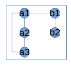
(a) Active constraint graph used to label a 2D node in (b); $(a_{1},b_{1})$ is the sole active constraint edge.

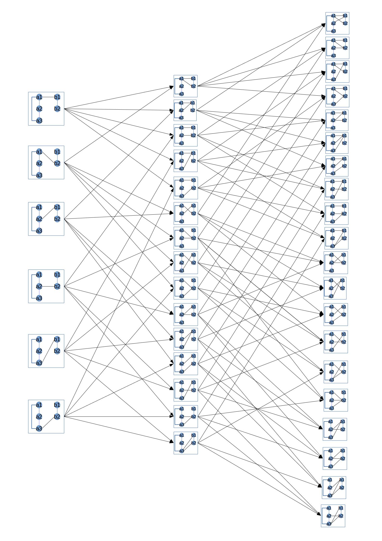
(b) Stratification DAG of Ex. Toy3.

Figure 1: Atlas (stratification) of the (toy-sized) configuration space of Ex. Toy3 of Section 2.1.1. (b) The nodes of the DAG represent active constraint regions and DAG edges connect a region to a boundary region, one dimension lower. Each node box displays the active constraint graph of its corresponding region. The nodes in the leftmost column represent 2D active constraint regions, i.e., they contain configurations with two degrees of freedom. Adding an active constraint edge, yields 1D active constraint regions (center column). Adding one more edge yields 0D regions, each containing finitely many rigid configurations (rightmost column).

\begin{overpic}[scale={.3},tics=10]{./sections/fig/Input_white.png} \put(20.0,60.0){\color[rgb]{0,0,1}{$A$}} \put(53.0,60.0){\color[rgb]{0,1,0}{$B$}} \end{overpic}

(a) Input to Problem ($C_{1}$, $C_{2}$).

\begin{overpic}[scale={.3},tics=10]{./sections/fig/CayleySpaces_white.png} \put(50.0,75.0){\color[rgb]{0,0,255}{1D Cayley}} \put(75.0,35.0){\color[rgb]{0,0,255}{1D Cayley}} \put(75.0,28.0){\color[rgb]{0,0,255}{1D node}} \put(76.0,20.0){\color[rgb]{0,150,0}{2D Cayley}} \put(76.0,15.0){\color[rgb]{0,150,0}{with hole}} \put(55.0,38.0){\color[rgb]{0,150,0}{2D node}} \put(8.0,80.0){\color[rgb]{200,146,0}{3D Cayley}} \put(48.0,5.0){\color[rgb]{200,146,0}{3D Cayley}} \put(42.0,15.0){\color[rgb]{200,146,0}{3D node}} \put(5.0,10.0){\color[rgb]{1,0,0}{4D node}} \end{overpic}

(b) Active constraint regions in the atlas represented as nodes colored by their dimension, shown with their Cayley configuration spaces (see full caption below).

\begin{overpic}[scale={.3},tics=10]{./sections/fig/ACG_white.png} \put(69.0,18.0){\color[rgb]{0,0,255}{5 active}} \put(65.0,14.0){\color[rgb]{0,0,255}{constraints}} \put(75.0,28.0){\color[rgb]{0,0,255}{1D node}} \put(48.0,27.0){\color[rgb]{0,150,0}{4 active}} \put(46.0,23.0){\color[rgb]{0,150,0}{constraints}} \put(40.0,37.0){\color[rgb]{0,150,0}{2D node}} \put(20.0,2.0){\color[rgb]{200,146,0}{3 active constraints}} \put(42.0,15.0){\color[rgb]{200,146,0}{3D node}} \put(5.0,10.0){\color[rgb]{1,0,0}{4D node}} \end{overpic}

(c) Active constraint regions in the atlas represented as nodes colored by their dimension, shown with their active constraint graphs.

\begin{overpic}[scale={.25},tics=10]{./sections/fig/Sweeps_white.png} \put(15.0,85.0){\color[rgb]{200,146,0}{sweep views of different flips}} \put(75.0,25.0){\color[rgb]{0,0,255}{1D node}} \put(40.0,40.0){\color[rgb]{0,150,0}{2D node}} \put(18.0,17.0){\color[rgb]{200,146,0}{3D node}} \put(0.0,10.0){\color[rgb]{1,0,0}{4D node}} \end{overpic}

(d) Active constraint regions in the atlas represented as nodes colored by their dimension, shown with Cartesian configuration sweep views(see full caption below).

Figure 2: (b), (c), and (d) show different views of a portion of the atlas centered on a 2D active constraint region. (b) The grid of little cubes next to each node delineates the Cayley configuration space of that region. Each little cube is a Cayley point or a Cayley configuration. Consider the 2D active constraint region in the center. This region has has no Cayley points in the middle (a hole) since every realization of these Cayley points violates $C_{1}$. These violations are caused by point pairs that are neither Cayley parameters nor edges of the active constraint graph. Such hole regions typically also have a convex Cayley parametrization. The Cayley points highlighted with a different color are points adjacent to their child (boundary) regions albeit using different Cayley parameters. (d) Each sweep view is the union of realizations, one per Cartesian configuration in the corresponding node. Each sweep view shows a different flip (defined in Section 2.3.2) of the Cayley configuration space of the corresponding node.

The EASAL software is based on the theoretical concepts described in this section. We explain and illustrate EASAL’s three strategies below. The reader will find the video at http://www.cise.ufl.edu/∼sitharam/EASALvideo.mpg useful to understand the following.

2.1 Strategy 1: Atlasing and Stratification

EASAL’s first strategy is to partition and stratify the Cartesian configuration space into regions $R$ called the active constraint regions, each labeled by its active constraint graph (See Fig. 1(a)). Consider the set of points participating in the active constraints that define $R$. Let $V_{R}$ be any minimal superset of points that supports additional constraints, of type $C_{2}$, to locally fix (generically rigidify) the two point-sets with respect to each other. Now, $V_{R}$ is taken to be the set of vertices of the active constraint graph of $R$. An edge of the active constraint graph represents either (i) one of the active constraints that define $R$ or (ii) a vertex pair in $V_{R}$ that lies in the same point-set $A$ (or $B$) in Problem ($C_{1}$, $C_{2}$). Notice that building the active constraint graph of $R$ reduces to picking a minimal graph isomorph from Fig. 4 containing the active constraints that define $R$.

The active constraint regions are organized as a partial order (directed acyclic graph or DAG, see Fig. 1(b) and Fig. 2(c)), that captures their dimensions and boundary relationships. In particular, the active constraint graph of a region is a subgraph of the active constraint graph of its boundary regions; and the co-dimension of a region is generically the number of active constraint edges. The analysis of the graph benefits from the following concepts of combinatorial rigidity (we additionally refer the reader to [19]).

A linkage is a graph, $G=(V,E)$, of vertices and edges, with an assignment of lengths, $\gamma:E\rightarrow\mathbb{R}$, for each edge. A (Euclidean) realization of a linkage in $\mathbb{R}^{3}$ is an assignment of points in $\mathbb{R}^{3}$ to vertices (factoring out the three rotations and three translations of SE(3)) such that the Euclidean distance between pairs of points are the given edge lengths $\gamma$. A realization is said to be rigid if there is no other realization in its neighborhood that has the same edge lengths. A graph is said to be rigid if a generic linkage realization of the graph is rigid. Otherwise, the graph is said to be flexible (not rigid). A rigid linkage generically has finitely many realizations. A graph is said to be minimally rigid, well constrained or isostatic if it is rigid and the removal of any edge causes it to be flexible. When the realization is rigid, all non-edges have locally fixed lengths and are said to be locally implied or dependent. If the graph $G$ arises as an active constraint graph for Problem ($C_{1}$, $C_{2}$) with the active constraint edges being assigned length intervals, we obtain an active constraint linkage. In this paper we treat active constraint linkages just like linkages while analyzing generic rigidity properties.

(a) 20 atom input

\begin{overpic}[scale={.2},tics=10]{./sections/fig/sweepview.eps} \put(56.0,76.0){\color[rgb]{0,0,0}\vector(1,1){18.0}} \put(36.0,73.0){\color[rgb]{0,0,0}\vector(1,3){8.0}} \put(20.0,100.0){\color[rgb]{0,0,0}{$T(B)$ sweep}} \put(73.0,95.0){\color[rgb]{0,0,0}{$A$ fixed}} \end{overpic}

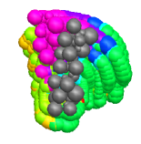
(b) Realization sweep view

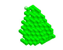
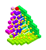
(c) Cayley configuration space view

Figure 3: Realization sweep view and Cayley configuration view of Ex. Toy20. (b) Sweep of realizations $T(B)$ for fixed $A$ in a 3D active constraint region. (b,right) Same view with $T(B)$ color coded to show realizations adjacent to lower dimensional boundary regions where a new constraint becomes active. (c) Each cube represents one Cayley configuration with at least one realization. (c,right) Only those Cayley points adjacent to child boundary regions are color coded as in (b, right), except for the yellow ones, shown as icosahedra, which are placed there as witness points (see Sections 3.1, 3.3.1 and 3.4.1) by parent regions, since this region is a boundary of those parent regions.

The degrees of freedom (dof) of a graph (linkage) is the minimum number of edges whose addition, generically, makes it rigid. Thus, the number of degrees of freedom is the same as the generic (effective) dimension of the realization space of a (active constraint) linkage of the graph. In $\mathbb{R}^{3}$, Maxwell’s theorem [41] states that rigidity of a graph $G=(V,E)$, implies that $|E|\geq 3|V|-6$ (in $\mathbb{R}^{2}$, $|E|\geq 2|V|-3$). If the edges are independent, this ensures minimal rigidity.

Note (Genericity Assumption): When $k=2$, the effective dimension of an active constraint region plus the number of active constraints is always 6, i.e., the number of active constraints generically determines the co-dimension of the region. This is because, in Problem ($C_{1}$, $C_{2}$), generically, implied non-edges are not active constraints, i.e., the active constraint edges are not implied by (dependent on) the rest of the active constraint graph. Inactive constraints (implied or not) do not restrict the dimension of active constraint regions. For the special case of Problem ($C_{1}$, $C_{2}$), in which sets $A$ and $B$ are centers of non intersecting spheres of generic distinct radii, these assumptions are an unproven conjecture, for which counterexamples haven’t been encountered. When the radii are all the same, simple counterexamples exist where implied non-edges are active constraints.

Employing these concepts, EASAL is able to use a classical notion called the Thom-Whitney stratification [38] of (effective) dimensional regions of a semi-algebraic set to stratify the configuration space atlas. In the atlas, DAG edges between two nodes indicate a boundary relationship: a lower dimensional child region is the boundary of a parent region one dimension higher (one fewer active constraint). Thus, the atlas is organized into strata, one for each (effective) dimension, and DAG edges exist only between adjacent strata. In Section 3.1, we describe in detail the algorithm used for atlasing and stratification of the configuration space.

2.1.1 Toy3

Consider Problem ($C_{1}$, $C_{2}$) in $\mathbb{R}^{2}$ with two point-sets $A$ and $B$; $A$ contains three points - $a_{1}$, $a_{2}$, and $a_{3}$ and $B$ contains two points - $b_{1}$ and $b_{2}$. The ambient space is SE(2) of dimension 3. A complete stratification of the realization space is shown in Fig. 1(b). The three strata are organized as a DAG, with nodes representing active constraint regions and labeled by their corresponding active constraint graphs. The vertices in the active constraint graph are points participating in the active constraints that define $R$. The edges are of two types, (i) between points in the same point-set and (ii) the active constraints, between points in different point-sets.

All regions in the leftmost column consist of configurations with two degrees of freedom and are called 2D nodes. Adding an extra active constraint to any of these nodes yields 1D nodes in the center column. By adding an extra active constraint to the nodes in the center column, we get the 0D nodes, shown in the rightmost column, each containing finitely many rigid configurations. A DAG edge represents a boundary relationship of the child region to a parent interior region one dimension higher.

2.2 Strategy 2: Recursive Search from Interior to Lowest Dimensional Boundary

To construct the atlas, EASAL’s second strategy is to recursively, using depth first search, start from the interior of an active constraint region and always locate boundaries or child regions of strictly one dimension less. The boundary or descendant regions of an active constraint region consist of configurations where new constraints become active and lead to the discovery of children active constraint regions. Fig. 3 shows the boundary regions in the Cayley and Cartesian configuration spaces for a typical 3D active constraint region in a toy-sized atlas.

In particular, a boundary region with one additional active constraint corresponds to 1 dimension less than the interior or parent region. Since EASAL only looks for boundaries one dimension less at every stage (boundary detection is explained in detail in Section 3.3), it has a higher chance of success than looking for the lowest dimensional active constraint regions directly (0D regions contain realizations of rigid active constraint linkages, that are sought as low energy configurations in the context of molecular and materials assembly).

Moreover, generically, if there is a region with the active constraint set $H\cup\{a\}\cup\{b\}$, then the region with active constraint set $H$ has at least two boundary or child regions, one with active constraint set $H\cup\{a\}$ and another with active constraint set $H\cup\{b\}$ as the active constraints. Both of these are parents of the region with active constraint set $H\cup\{a\}\cup\{b\}$.

Because of this, when a new region is found, all its ancestor regions can be discovered. So, even if a “small” (hard-to-find) region is missed at some stage, if any of its descendants are found at a later stage, say via a larger (easy-to-find) sibling, the originally missed region is discovered.

2.3 Strategy 3: Cayley Convexification for Efficient Search and Realization

Locating a boundary region satisfying an additional active constraint is, off-hand, challenging due to the disconnectedness and complexity of Cartesian active constraint regions. To address this challenge, EASAL uses a theoretical framework developed in [52]. EASAL efficiently maps (many to one) a $d$-dimensional active constraint region, to a convex region of $\mathbb{R}^{d}$ called the Cayley configuration space. Convexity allows for efficient sampling and search for boundaries. In addition, it is efficient to compute the inverse map from each Cayley configuration to its finitely many corresponding Cartesian realizations or configurations. We describe this strategy in more detail below.

A complete 3-tree is any graph obtained by starting with a triangle and adding a new vertex adjacent to the vertices of a triangle in the current graph. Alternatively, this amounts to successively pasting a complete graph on 4 vertices (a tetrahedron) onto a triangle in the current graph. This yields a natural ordering of vertices in a 3-tree (we drop ‘complete’ when the context is clear). A 3-tree has $3|V|-6$ edges and hence, a 3-tree linkage is minimally rigid in $\mathbb{R}^{3}$. That is, a 3-tree generically has finitely many realizations, and removing any edge gives a flexible partial 3-tree.

One way to represent the realization space of a flexible partial 3-tree linkage is by choosing non-edges (called Cayley parameters) that complete it to a 3-tree. Then, given a partial 3-tree linkage and length values for the chosen Cayley parameters there are only finitely many realizations for the resulting rigid 3-tree linkage. Since finitely many Cartesian realizations correspond to a single Cayley configuration (tuple of Cayley parameter values), the Cayley parametrization is a many to one map from the Cartesian realization space to the Cayley configuration space. The inverse map can be computed easily by solving three quadratics at a time as explained in Section 3.4. Therefore, if the Cayley configuration space were convex, it, and thereby the Cartesian realization space, can be efficiently sampled.

Theorem 1 below asserts that the length tuples of non-edge Cayley parameters $F$ (that complete a partial 3-tree into a 3-tree) form a convex set. Given a linkage with edges $H$ of length $l_{H}$ a chart for this linkage is defined by choosing a non-edge set $F$ with lengths $l_{F}$ such that the linkage with edge set $H\cup F$, and edge lengths $l_{H}$ and $l_{F}$ is realizable. Formally, the chart is the set $\{l_{F}:(H\cup F,l_{H},l_{F})$ is realizable in $\mathbb{R}^{3}\}$, denoted $\Phi_{F}(H\cup F,l_{H})$.

Theorem 1.

([52] Any partial 3-tree yields an exact convex chart) If an active constraint graph $G_{H}=(V,H)$ of an active constraint region $R$ is a partial 3-tree then, by adding edge set $F$ to give a complete 3-tree $G=(V,E=F\cup H)$, we obtain an exact convex chart $\Phi_{F}(G,H,l_{H})$ for $R$, in the parameters $F$. The exact convex chart $\Phi_{F}(G,H,l_{H})$ has a linear number of boundaries in $|G|$ defined by quadratic or linear polynomial inequalities. If we fix the parameters in $F$ in sequence, their explicit bounds can be computed in quadratic time in $|G|$.

As explained in [52], the theorem still holds when $H$ is an active constraint linkage i.e., when $l_{H}$ is a set of intervals rather than a set of fixed lengths. Besides proving Theorem 1 [52] shows the existence of convex Cayley configuration spaces for a much larger class of graphs (beyond the scope of this paper).

Furthermore, as elaborated in [53], for active constraint graphs arising between $k$ point-sets, generalized 3-trees yield convex configuration spaces. This is because each point-set represents a unique realization of their underlying complete graph. A generalized 3-tree is defined by construction similar to a 3-tree. However, during the construction, assume 3 or more vertices in the already constructed graph $G$ belong to the same point-set say $A$ of Problem ($C_{1}$, $C_{2}$). Now, if a new vertex $v$ is constructed with edges to the vertices of a triangle $T$ in $G$, then the $m\leq 3$ vertices in $A\cap T$ can be replaced by any other $m$ distinct vertices in $A$ to which $v$ is adjacent. Moreover, generalized 3-trees, just like 3-trees, have an underlying sequence of tetrahedra, and are rigid with finitely many realizations. Going forward, we simply refer to generalized (partial) 3-trees as (partial) 3-trees.

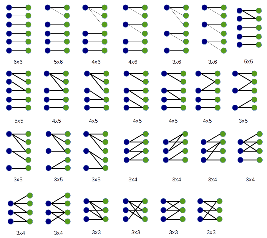
Figure 4: In each graph above, the vertices of the same color represent points in the same point-set $A$ (or $B$) in Problem ($C_{1}$, $C_{2}$) and form a complete graph (whose edges are not shown). Edges between vertices indicate point pairs whose distance is in the preferred interval, i.e., the constraint is active. For $k=2$, all active constraint graphs are isomorphic to subgraphs of the ones shown. The graphs above are rigid and correspond to generically rigid 0-dimensional active constraint regions. The label $m_{1}\times m_{2}$ below each active constraint graph indicates that $m_{1}$ points in the first point-set and $m_{2}$ points in the second point-set participate in the active constraints.

The quadratic and linear polynomials defined in Theorem 1 arise from simple edge-length (metric) relationships within all triangles and tetrahedra and are called tetrahedral inequalities, and the explicit bounds mentioned in the theorem are called tetrahedral bounds. EASAL leverages this efficient computation of the convex bounds enhanced by the Theorem 5.1.3 in [14], described in Section 3.2. It turns out that, for small $k$, almost all active constraint graphs arising from Problem ($C_{1}$, $C_{2}$) are partial 3-trees and thus their regions have a convex Cayley parametrization. Specifically (see Fig. 4), all the active constraint graphs with 1, 2 and 3 active constraints (5D, 4D and 3D atlas regions) are partial 3-trees. $86\%$ of active constraint graphs with 4 active constraints (2D atlas regions) and $70\%$ of active constraint graphs with 5 active constraints (1D atlas regions) are partial 3-trees. Since, regions with 6 active constraints (0D atlas regions) have finite realization spaces, Cayley parametrization is irrelevant. Section 3.4.1 describes how we find realizations when the active constraint graph is not a partial-3-tree.

Although most active constraint graphs have convex Cayley configuration spaces, the feasible region is a non-convex subset created by cutting out a region defined by other constraints of type $C_{1}$. Each such constraint is between a pair of points, one from each point-set, that is neither an active constraint nor a Cayley parameter in the active constraint graph. However, the regions that are cut out typically have a (potentially different) convex Cayley parametrization. This can be seen in Fig. 2(b) where the Cayley configuration space of the node in the center has a hole cut out because of constraint violations by point pairs that are neither Cayley parameters nor edges in the active constraint graph.

2.3.1 Toy3 contd

Here, the active constraint graph shown in Fig. 1(a) is used to illustrate Cayley convexification. Since that example is in $\mathbb{R}^{2}$, 2-trees serve the purpose of 3-trees used in EASAL [52]. A complete 2-tree is any graph obtained by starting with an edge and successively pasting a triangle onto an edge in the current graph. A partial 2-tree is any subgraph of complete 2-tree.

Consider the partial 2-tree linkage shown in Fig. 5 (left). To represent the configuration space of this flexible linkage, we add the non-edges $e1$ and $e2$, shown with dotted lines, to complete the 2-tree. This not only makes the linkage rigid, but its realization is easy by a straightforward ruler and compass construction, solving two quadratics at a time. The non-edges $e1$ and $e2$ are the Cayley parameters and correspond to independent flexes. Fig. 5 (right) shows the convex Cayley configuration space corresponding to this linkage.

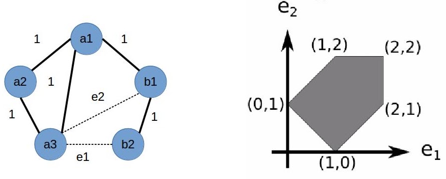
Figure 5: Ex. Toy3 viewed as (left) a linkage in $\mathbb{R}^{2}$ (see text for description). (right) The 2D convex Cayley configuration space for the linkage and the chosen Cayley parameters $e1$ and $e2$. The shaded area delineates the realizable lengths of $e1$ and $e2$.

If the edges in the graph in Fig. 5 (left) were assigned length intervals instead of fixed lengths, yielding an active constraint linkage, the resulting configuration space would continue to be convex, but would be 7 dimensional. However, when these intervals are relatively small in comparison to the edge lengths, the Cayley configuration space remains effectively 2 dimensional.

2.3.2 Realization: Computing Cartesian Configurations from a Cayley Configuration

The addition of the Cayley parameter non-edges to the active constraint graph yields a complete 3-tree. This reduces computation of the Cartesian realizations of a Cayley configuration (a tuple of Cayley parameter length values) to realizing a complete 3-tree linkage. Realizing a complete 3-tree linkage with $i$ tetrahedra reduces to placing $i$ new points one at a time using 3 distance constraints between a new point and 3 already placed points. For each new point we solve the quadratic system for intersecting 3 spheres resulting in two possible placements of the new point. This yields $2^{i}$ possible realizations of the Cayley configuration. A flip associated with the Cayley configuration space consists of Cartesian realizations of all Cayley configurations restricted to one of these $2^{i}$ placements [53].

3 Algorithmic Ideas and Implementation

This section discusses the key algorithmic ideas implemented in EASAL. EASAL starts by generating all possible active constraint graphs with 1 or 2 (depending on user input) active constraints yielding 5D or 4D regions (represented as root nodes) in the atlas and then successively samples them. The main algorithm, ALGORITHM 1 merges the three strategies described in the previous section.

sampleAtlasNode

input : atlasNode: node

output : Complete sampling of the atlasNode and all its children

$H$ = node.activeConstraints

$G_{H}$ = node.activeConstraintGraph

if  $G_{H}$ is minimally rigid then

      stop;

end if

$F$ = complete3Tree($G_{H}$)

$C$ = computeConvexChart($G_{H}$, $F$)

for  each cayleyPoint $p$ within convexChart $C$  do

       $R$ = computeRealizations($p$)

      

      for  each realization $r$ in $R$ do

             if !aPosterioriConstraintViolated($r$) then

                   if  isBoundaryPoint($r$) && hasNewActiveConstraint($r$, $G_{H}$)  then

                         $e$ = newActiveConstraint($r$, $G_{H}$);

                         $G^{\prime}$ := $G_{H\cup\{e\}}$ ;

                         if  $G^{\prime}$ is not already present in the current atlas then

                               childNode = new atlasNode($G^{\prime}$)

                               childNode.insertWitness($p$);

                               sampleAtlasNode(childNode);

                              

                         end if

                        else

                               childNode = findNode($G^{\prime}$);

                         end if

                        node.setChildNode(childNode);

                   end if

                  

             end if

            

       end for

      

end for

ALGORITHM 1 High level EASAL pseudocode

ALGORITHM 1 proceeds as follows. It (i) recursively (by depth first search) generates the atlas by discovering active constraint regions of decreasing dimension; (ii) uses Cayley convexification of the region to efficiently compute bounds for Cayley parameters a priori (before realization), and samples Cayley configurations in this convex region; (iii) detects boundary regions of 1 dimension less a posteriori (after realization) i.e., when a new constraint becomes active, and efficiently finds the (finitely many) Cartesian realizations of the Cayley configuration samples. We describe each of these aspects of the algorithm in Sections 3.1, 3.2 and 3.3 respectively.

3.1 Atlasing and Stratification

EASAL stores and labels regions of the Cartesian configuration space as an atlas as described in Section 2.1. The regions of the atlas are stored as nodes of a directed acyclic graph, whose edges represent boundary relationships. Each region of the atlas is an active constraint region associated with a unique active constraint graph $G_{H}$, where $H$ is the set of active constraints (see Algorithm 1).

The exploration of the atlas is done by the recursive sampleAtlasNode algorithm using one of the generated atlas root nodes as input. Using depth first search, this algorithm samples the atlas node and all its descendants. Fig. 6 gives an overview of the algorithm.

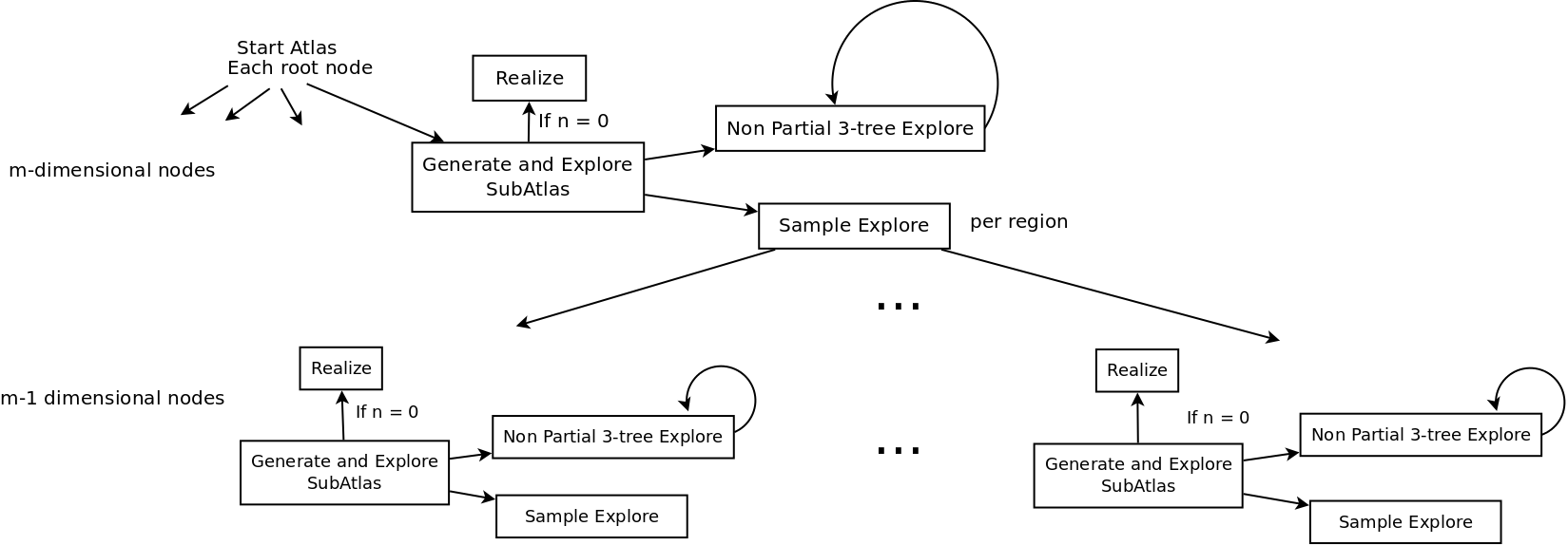
Figure 6: A high level flowchart of the algorithm for generating and exploring the atlas

Base case of recursion: If active constraint graph $G_{H}$ of the node is minimally rigid i.e., the active constraint region is 0D, then there is only 1 Cayley configuration (with finitely many Cartesian realizations). We have no more sampling to do, hence return.

The recursion step: If $G_{H}$ is not minimally rigid, EASAL applies the complete3Tree algorithm of in Section 3.2 to find a set of parameters $F$ to form a 3-tree. This leverages the convex parametrization theory [52] of Section 2.3 and ensures that a linkage with edge set $H\cup F$ is minimally rigid and easily realizable.

Next EASAL finds the convex chart for the parameters $F$ via the computeConvexChart algorithm. This algorithm leverages Theorem 1 enhanced by the theory presented in [14]. This algorithm, detects the tetrahedral bounds and samples uniformly within this region using a user specified step size. Detection of the tetrahedral bounds is explained in more detail in Section 3.2.

Next we compute the Cartesian realization space of the convex chart using the computeRealization algorithm (described in Section 3.4). This uses two nested for loops. The outer loop runs for each Cayley point $p$ in the convex chart and computes the realizations for each of these points as described in Section 2.3.2. The inner loop runs for each realization $r$ of the point $p$ and detects whether some Cayley points violate constraints between pairs that do not form an edge of active constraint graphs. This is the crucial test that indicates that a new constraint has become active. The Cayley point whose realization caused a child boundary region to be found at a parent is called a witness point, since it witnesses the boundary, and is placed in the child boundary region clearly labeled as a witness point coming from each parent region (see also Figure Fig. 3 and Section 3.4.1). We perform the aPosterioriConstraintViolated check (described in Section 3.3) to discover a boundary region. For every new region discovered in this manner, we sample the region recursively with the sampleAtlasNode algorithm.

3.2 Cayley Convexification and A Priori Computation of Bounds

According to the theory of convex Cayley parametrization in Section 2.3, if the active constraint graph of an active constraint region is a partial 3-tree, choosing non-edges that complete the partial 3-tree into a complete 3-tree as Cayley parameters always yields a convex Cayley space. In other words, the active constraint linkage has a convex Cayley configuration space if it is a partial 3-tree. Computing the bounds of this convex region ensures that sampling stays in the feasible region and minimizes discarded samples.

The first step is thus to find the set of Cayley parameters that complete a partial 3-tree. This is done by the complete3Tree algorithm. The complete3Tree algorithm uses Theorem 1 of Section 2.3. It first creates a look-up table containing all possible complete 3-trees. Given a graph $G_{H}$ as the input, we find a graph in the look-up table so that $G_{H}$ is a proper subgraph of either the graph or one of its isomorphisms. The set of edges by which $G_{H}$ differs from the graph found in the look-up table is returned as $F$. $F$ is the set of Cayley parameters.

Finding bounds for each Cayley parameter (bounds on edge lengths for $F$) has two cases:

• If there is only one Cayley parameter in a tetrahedron, the tentative range of that parameter is computed by the intersection of tetrahedral inequalities.

• If there is more than one unfixed Cayley parameter in a tetrahedron, then the tentative ranges of a parameters are computed in a specific sequence [14]. The tentative range of a parameter in the sequence is computed through tetrahedral inequalities using fixed values for the parameters appearing earlier in the sequence. Since the range of the parameter is affected by the previously fixed parameters, more precise range computation of the unfixed parameter is required for every iteration/assignment of fixed parameters.

The actual range for each parameter is obtained by taking the intersection of the tentative range and the range of $C_{2}$. The order in which Cayley parameters are fixed have an effect on the efficiency of the range computation [14]. We pick parameters in the order that gives the best efficiency. Once we choose the parameters $F$ and the sequence, the explicit bounds can be computed in quadratic time in $|G|$. Once explicit bounds for each Cayley parameter have been found, we populate this region by sampling it uniformly using a user specified step size.

3.3 Boundary Region Detection

The boundary regions of an active constraint region caused by newly active constraints can be detected only after Cartesian realizations are found using the computeRealization algorithm (described later in this section).

If the newly active constraint occurs between a point pair that is a Cayley parameter, then this is immediately detected at the start of sampling from the a priori bounds computation of the convex Cayley region. In particular, if (i) the actual range of a Cayley parameter $p$ for a region $r$ includes either the lower or upper bound $\overline{p}$ of Problem ($C_{1}$, $C_{2}$) and (ii) a Cayley point with $p=\overline{p}$ has a realization, then that Cayley point is on a boundary region of $r$. Otherwise, if a newly active constraint occurs between a pair that is not a Cayley parameter, then the corresponding boundary is detected as follows.

3.3.1 A Posteriori Boundary or New Active Constraint Detection

A posteriori boundary detection involves checking for violation of constraints corresponding to pairs that are neither edges nor Cayley parameters in the active constraint graph. EASAL relies on Cayley parameter grid sampling to find the child boundary regions of each active constraint region. However, boundary detection is not guaranteed by Cayley parameter grid sampling alone, since the sampling step size may be too large to identify a close-by point pair that causes a newly active constraint. That is, the constraint violation could occur between 2 feasible sample realizations or between a feasible and an infeasible realization on the same flip in the sampling sequence. In the former case, the missed boundary region is “small.” However, due to the precise structure of Thom-Whitney stratification, it is detected if any of its descendants is found via a larger sibling (as described in detail in Section 2.2). In the latter case, the newly active constraint has been flagged but exploration (by way of binary search) is required to find the exact Cayley parameter values at which new constraints became active. The binary search is on the Cayley parameter value, with direction determined by whether the realization is feasible or not.

In both cases, once a new active constraint $e$ is discovered, we add the new constraint to $G_{H}$ and create an new active constraint graph $G^{\prime}=G_{H\cup\{e\}}$. Notice that a boundary region could be detected via multiple parents. However, since regions have unique labels, namely the active constraint graphs, no region is sampled more than once. If $G^{\prime}$ has already been sampled, we just add the node for $G^{\prime}$ into the atlas, as a child of $G_{H}$. Otherwise, we create a new atlas node with $G^{\prime}$, sample it using the recursive sampleAtlasNode algorithm and then add it as a child of $G_{H}$. In both cases, the parent leaves one or more witness Cayley points in the child region (see Figure 3 and Sections 3.1 and 3.4.1).

3.4 Cartesian Realization

The computeRealization algorithm used to find realizations takes in an active constraint region and its convex chart and generates all possible Cartesian realizations. As stated earlier, each Cayley configuration can potentially have many Cartesian realizations or flips. There are 2 cases depending on whether the active constraint graph is a partial 3-tree or not. Cartesian realization for partial 3-trees is straightforward as described in Section 2.3.2. We describe the other case in detail next.

3.4.1 Cartesian Realization for Non-partial 3-trees: Tracing Rays

According to Section 2.3, active constraint regions without a partial 3-tree active constraint graph occur rarely. To find tight convex charts that closely approximate exact charts, we first drop constraints one at a time, until the active constraint graph becomes a partial 3-tree. In doing so, we end up in an ancestor region, with a partial 3-tree active constraint graph and a convex Cayley parametrization. Note that since non-partial 3-trees potentially arise only when we are exploring active constraint regions with 4 or 5 active constraints (2D and 1D atlas nodes respectively), it is always possible to drop one or two constraints to reach an ancestor region which has a partial 3-tree active constraint graph. We do not explore 0D regions. They consist of a single Cayley configuration with only finitely many realizations, which are found when the region is found.

Once in the ancestor region, we trace along rays to populate the lower dimensional region by searching in the ancestor region. For example, to find a 2D boundary region which does not have a partial 3-tree active constraint graph or a convex parametrization, we drop one constraint. We then uniformly sample the 3D region guaranteed to have a convex parametrization (setting the third coordinate to zero). For each sample point, we traverse the third coordinate using binary search (Section 3.3.1). This generalizes to any dimension and region in the sense that ray tracing is robust when searching for and populating a region one dimension lower. By recursing on the thus populated region, we find further lower dimensional regions.

3.5 Complexity Analysis

The highest dimension of an active constraint region for $k=2$ is 6. More generally, for $k$ point-sets, the maximum dimension of a region is $6(k-1)$. If $r$ regions of dimension $d$ have to be sampled, EASAL requires time linear in $r$ and exponential in $d$. Specifically, given a step size $t$ (a measure of accuracy) as a fraction of the range for each Cayley parameter, the complexity of exploring a region is $O((\frac{1}{t})^{6(k-1)})$. This indicates a tradeoff between complexity and accuracy [44].

The complexity is also affected by $n$ the number of points in each point set. This is due to a posteriori constraint checks which involve checking every point pair (one from each point set) for violation of $C_{1}$. Thus, the complexity of exploring a region is $O((\frac{1}{t})^{6(k-1)}\times n^{2})$.

If $r$ is the number of regions to explore, given as part of the input by specifying a set of active constraints of interest, the complexity of exploring all these regions is $O(r\times(\frac{1}{t})^{6(k-1)}\times n^{2})$. In the worst case, $r$, can be as large as $O(k^{2}\cdot n^{12k})$. In this case, we cannot expect better efficiency, since the complexity cannot be less than the output size. Usually, $r$ is much smaller $O(k^{2}\cdot n^{12k})$, since much fewer active constraint regions are generally specified as part of the input.

4 Results

In this section we briefly survey experimental results appearing in [53, 42, 60], that illustrate some of EASAL’s capabilities. The main applications of EASAL are in estimating free-energy, binding affinity, crucial interactions for assembly, and kinetics for supramolecular self-assembly starting from rigid molecular motifs e.g., helices, peptides, ligands etc.

4.1 Atlasing and Paths

$n$	Step size(as a fraction of the smallest radius)	Number of Regions	Number of samples	Good Samples	Time(in minutes)
6	0.25	26k	1.9 million	1.3 million	82
6	0.375	23k	617k	379k	23
6	0.5	19k	289k	172k	11
20	0.25	184k	5.8 million	716k	335
$20^{*}$	0.25	206	63k	22k	2
$20^{\dagger}$	0.25	3107	74k	33k	7

Table 1: Time on a standard laptop (see text) to stratify the configuration space of pairwise constrained point-sets with the tolerance set to $(1.0-0.75)\times$ sum of radii. The input point-set with $n=6$ is Ex. 6Atom and the $n=20$ input is Ex. Toy20. Note that in $20^{*}$, only one 5D and its children 4D regions are sampled and in $20^{\dagger}$, only one 5D and its descendant 4D and 3D region are sampled.

In this section, we survey numerical results from experiments in [53], illustrating the performance of EASAL in generating an atlas and computing paths for the configuration space of two ($k=2$) input point-sets. The experiments were run on a machine with Intel(R) Core(TM) i7-7700 @ 3.60GHz CPU with 16GB of RAM. These results can be reproduced by the reader using the accompanying EASAL software implementation (see Section 2.4 of the User Guide for instructions).

The time required for generating the atlas is measured for a given accuracy of coverage, measured in terms of the step size, and a given tolerance, which is the width of the interval in $C_{2}$. Two different input point-sets (Ex. 6Atom and Ex. Toy20) are used as input. The results for the $n=6$ input (Ex. 6Atom) show the time and number of samples for generating the atlas of all possible combinations of active constraint regions with one active constraint (5D atlas root nodes). The results for $n=20$ input (Ex. Toy20) show the time and number of samples required to generate the atlas for a typical randomly chosen 5D active constraint region and all its children. Also note that in $20^{*}$, only one 5D and its children 4D regions are sampled, and in $20^{\dagger}$, only one 5D and its descendant 4D and 3D regions are sampled. Ex. Toy20 is challenging due to the number of “pockets” in the point-set structure leading to a highly intricate topology of the configuration space with many effectively lower dimensional regions. Table 1 summarizes the results. These results can be reproduced using the test driver submitted (see Section 2.4 of the user guide).

4.1.1 Finding Neighbor Regions

\begin{overpic}[scale={0.4},tics=10]{./sections/fig/BoundingRegionsVertical.jpg} \put(28.0,85.0){\color[rgb]{0,0,1}{Sweeps}} \put(48.0,85.0){\color[rgb]{1,0,0}{4D node}} \put(56.0,60.0){\color[rgb]{200,146,0}{3D node}} \put(55.0,37.0){\color[rgb]{0,1,0}{2D node}} \put(52.0,25.0){\color[rgb]{123,104,238}{1D node}} \put(48.0,5.0){\color[rgb]{219,48,122}{0D node}} \put(60.0,85.0){\color[rgb]{0,0,0}{Constraint Graph}} \end{overpic}

Figure 7: A portion of a toy-sized atlas. The ancestor and descendant regions, of dimension four or less, of an active constraint region with 5 active constraints (which is a 1D atlas region, shown here as a blue line). The pink nodes represent its 0D child regions, the green nodes represent its 2D parent regions, the beige nodes represent its 3D grandparent regions and the red node represents its 4D ancestor region. Next to each node is shown its corresponding active constraint graph and the sweep views of two flips. The increasing number of constraints reduces the potential energy of the assembly.

For any given active constraint region, one of EASAL’s implemented functionalities gives all of its neighbor regions. A higher dimensional neighbor (parent) region has one active constraint less and a lower dimensional neighbor (child) region has one more active constraints. The atlas contains information on child and parent regions of every active constraint region.

If EASAL has been run using just the backend, the atlas information can be accessed from the RoadMap.txt file in the data directory. The neighbors are listed as “Nodes this node is connected to” at the end of each node’s information.

In the optional GUI (not part of TOMS submission), the neighbors of a region are listed in the Cayley space view. The GUI contains a feature called ‘Tree’, which additionally shows all the ancestors and descendants of an active constraint region. Fig. 7 shows the ‘Tree’ feature being used on an active constraint region having 5 active constraints. The figure shows each ancestor and descendant node along with their active constraint graphs and sweep views of Cartesian configurations in the region.

4.1.2 Finding Paths between Active Constraint Regions

The atlas output by EASAL can be used to generate all the paths between any two active constraint regions along with their energies. Once the atlas has been generated, finding paths is extremely fast as we discuss below.

Of particular interest is finding paths between two configurational regions with zero degrees of freedom or with 6 active constraints. These are the 0D nodes of the atlas with effectively rigid configurations. They find paths in which the highest number of degree of freedom level is bounded. In particular, paths through regions with 5 active constraints with one step higher degree of freedom and one fewer constraint. These regions represent a generic one degree of freedom motion path (see Fig. 8).

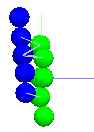
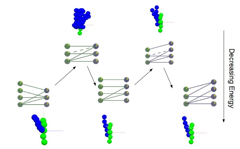
Figure 8: A path in a toy-sized atlas. The path connects two active constraint regions (left to right), each with 6 active constraints. The path traverses regions with at most one less constraint. Each active constraint region is labeled by its corresponding active constraint graph. The arrows form a path, losing or gaining a new active constraint, from the source to the destination active constraint regions. The sweep view of feasible configurations of a sample flip is shown next to each active constraint region. The left inset figure (Ex. 6Atom) shows the input molecules used for this experiment.

$n$	$r$	Average length of shortest path	Average time (see text) to find shortest path
6	176	7	1.9 ms
6	145	6	2.2 ms
20	787	18	119ms

The time on a standard laptop (see text), to find the shortest path between two active constraint regions with 6 active constraints through $m$ other active constraint regions with 5 or 6 active constraints.

$n$	$r$	$t$	Average time (see text) to find number of paths
6	176	2	2.02 s
	176	4	4 s
	176	8	6.04 s
	176	10	8.08 s
20	787	2	6 min
	787	4	11.58 min
	787	8	18.04 min
	787	10	27.44 min

The time on a standard laptop (see text), to find the number of paths of length $t$, between all pairs of active constraint regions with 6 active constraints, in a toy atlas with $r$ active constraint regions with 6 active constraints.

Table 2: Finding paths between active constraint regions

This experiment was performed on two example point-sets with $n=6$ (Ex. 6Atom) and $n=20$ (Ex. Toy20). In the first experiment, the shortest path between 100 randomly chosen pairs of active constraint regions with 6 active constraints are found. As shown in Table 2, for the $n=6$ example input, it took an average of 2 ms to find the shortest path, and the average length of the shortest path was 6. For the $n=20$ example input, it took an average of 119 ms to find the shortest path with the average length of the shortest path being 18. These results can be reproduced using the test driver (see Section 2.4 of the user guide)

In the second experiment, the number of paths of length $t$ in a toy atlas between all pairs of active constraint regions are found. This toy atlas had $r$ active constraint regions with 6 active constraints. As shown in Table 2, for the example input with $n=6$, the number of paths of length 10 were found in 8 seconds and the number of paths for the $n=20$ input in 27 minutes. These results can be reproduced using the test driver (see Section 2.4 of the user guide)

4.2 Coverage and Sample Size Compared to MC

In this section we sketch results from [42] comparing EASAL and its variants to the Metropolis Markov chain Monte Carlo (MC) algorithm for sampling a portion of the landscape of two point-sets arising from protein motifs (transmembrane helices, Ex. Toy20). In that paper, the effectiveness of EASAL in sampling crucial but narrow, low effective dimensional regions is demonstrated by showing that EASAL provides similar coverage as the traditional methods such as MC but with far fewer samples. For determining coverage, it is sufficient to sample only the interior of an active constraint region having 1 active constraint, without generating its children.

EASAL variants EASAL-1, EASAL-2, EASAL-3, and EASAL-Jacobian differ in their sampling distributions in the Cayley space and by extension in the Cartesian space. EASAL-1 samples the Cayley space uniformly. Since energy is directly related to distance, this does uniform sampling across energy levels. This however, skews the sampling in the Cartesian space. EASAL-2 uses a step size inversely proportional to the Cayley parameter value. This samples more densely in the interiors of the active constraint region and near tetrahedral bounds. This is useful if we want to sample densely at places where degeneracies such as flip intersections (so called conformational shifts and tunneling) are likely to occur. EASAL-3 uses a step size linearly proportional to the Cayley parameter value. This samples densely close to the boundaries. This is useful if we want to sample densely at lower energy values. EASAL-Jacobian uses a sophisticated adaptive Cayley sampling method to force uniform sampling in the Cartesian space. This is essential to compute volumes and thereby entropy and free energy accurately. A comparison of how sampling in the Cayley space relates to sampling in the Cartesian space, for these variants of EASAL, is shown in Fig. 9.

sampling method	EASAL-1	EASAL-2	EASAL-3	EASAL-Jacobian	MC	MultiGrid
$\varepsilon$-coverage	$\lceil 0.97\rceil$	$\lceil 1.14\rceil$	$\lceil 1.20\rceil$	$\lceil 0.66\rceil$	$\lceil 0.31\rceil$	N/A
Coverage percentage	92.06%	92.42%	74.08%	99.53%	99.96%	N/A
Number of Samples	100k	40k	30k	1 million	100 million	12 million
Ratio percentage	3.56%	5.17%	2.97%	3.45%	1.29%	N/A

Table 3: Comparison of EASAL variants with MC with respect to coverage and number of samples for the two transmembrane helices shown in Fig. 3(a) [42]. Here, $\varepsilon$ is computed as described in the text.

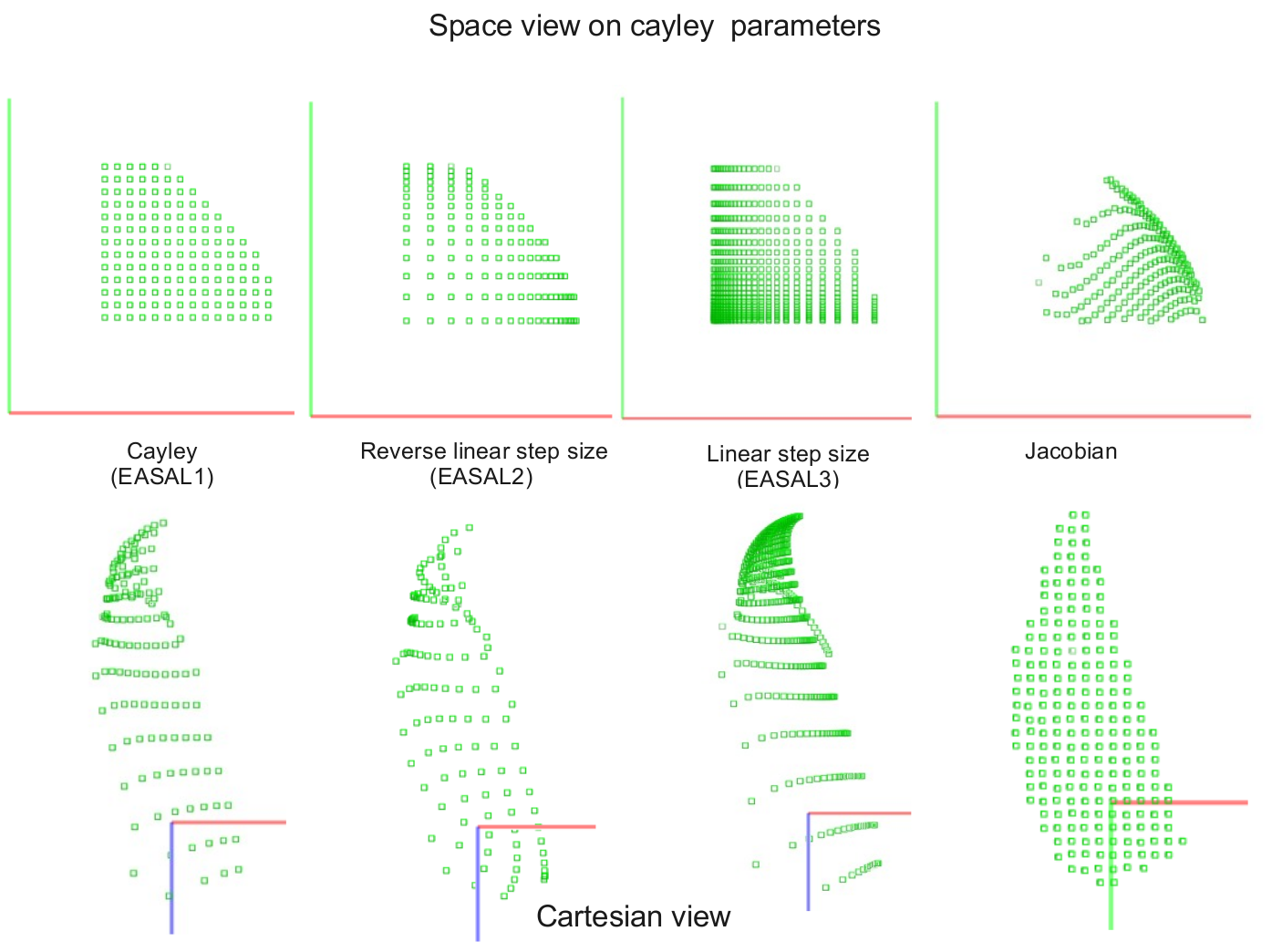
Figure 9: Comparison of sampling in Cayley v/s Cartesian space in variants of EASAL for a 2D active constraint region in the atlas for the example in Fig. 3(a) [42]. The axes in the top figure are the two Cayley parameters. In the bottom figure, the projection is on the $xy$ coordinates of the centroid of the second point-set with the centroid of the first point-set fixed at the origin.

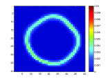
(a) MC

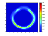
(b) MultiGrid

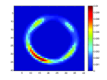
(c) EASAL-1

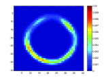
(d) EASAL-2

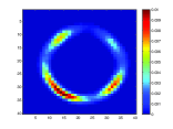
(e) EASAL-3

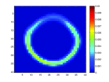
(f) EASAL-Jacobian

Figure 10: Projection in $\mathbb{R}^{2}$ of a configuration space for the example point-set shown in Fig. 3(a) as sampled by various methods. The projection is on the $xy$ coordinates of the centroid of the second point-set with the centroid of the first point-set fixed at the origin. The color scale on the right of each figure corresponds to the number of sampled points in a $\varepsilon$-sized cube centered around the grid point $(x,y)$. $\varepsilon$ is computed as described in the text [42].

The experiments were run on an Intel i5-2540 machine and the variants of EASAL were run on a Intel Core 2 Quad Q9450 @ 2.66 GHz. and a memory of 3.9 GB. With this setup, EASAL-1 took 3 hours 8 minutes. EASAL-2 took 4 hours 24 minutes, EASAL-3 took 10 hours 20 minutes, and EASAL-Jacobian took 14 hours 22 minutes. The methods were compared based on a their sampling coverage of a grid. The grid was set up to be uniform in the Cartesian configuration space and its bounds along the $X$ and $Y$ axes were -20 to 20 Angstroms, and along the $Z$ axes were -3.5 to 3.5 Angstroms.

The input in the experiment was as follows:

1. The two point-sets in the form of two rigid helices. Note that this is the special case of Problem ($C_{1}$, $C_{2}$) where the points are sphere centers.

2. The lower bound of the pairwise distance constraint, for all sphere pairs $i,j$ belonging to different point-sets, $dist_{ij}>0.8\times(\rho_{i}+\rho_{j})$ where $i$ and $j$ are residues, $dist_{ij}$ is the distance between residues $i$ and $j$, $\rho_{i}$ and $\rho_{j}$ are the radii of residue spheres $i$ and $j$ respectively.

3. An optional global constraint is the inter helical angle between the principal axes of the two input helices, $\theta<30^{\circ}$. Here, $\theta=a~{}cos(uv)$ where $u$ and $v$ are the principal axis of each point-set, i.e., $u$ and $v$ are the dominant directions in which the mass is distributed, alternatively the eigenvectors of the inertia matrix.

Over 43.5 million grid configurations were generated to ensure at least one pair was an active constraint, i.e., $dist_{ij}<\rho_{1}+\rho_{2}+0.9$. Out of these, around 86% were discarded, leaving us with about 5.8 million ‘good’ samples.

The methods were compared based on the following parameters.

• The epsilon coverage: a measure of how many sample points are within an $\varepsilon$-sphere of each grid point. Since the ambient space has dimension 6, $\varepsilon$ is set to $(\text{number of grid points}/\text{number of sampling points})^{1/6}/2$.

• The coverage percentage, which is the percentage of the grid $\varepsilon$-covered by the sampling algorithm.

• The number of samples required to achieve the given $\varepsilon$-coverage.

• The ratio percentage: Let $s_{1}$ be the number of samples in a specific but randomly chosen 3 dimensional region and $s_{2}$ be the number of samples in all ancestor regions with 1 active constraint that lead to the 3 dimensional region. The ratio percentage is $\frac{s_{1}}{s_{2}}\times 100$.

The best method should have the highest epsilon coverage and coverage percentage with the fewest samples. As can be seen from Table 3, MC gives the best coverage but requires 100 million samples. By contrast EASAL-Jacobian gives about the same relative coverage with one million samples (1% of MC). EASAL-2 gives a very good coverage of 92.42% with only 40k samples (0.04% of MC). EASAL-2 also has the best ratio percentage beating even MC by a large margin. Fig. 10 shows a 2D projection of a configuration space as sampled by various methods for the example point-set shown in Fig. 3(a). The projection is on the $xy$ coordinates of the centroid of the second point-set with the centroid of the first point-set fixed at the origin. Multigrid shows grid sampling where lower dimensional regions are repeat sampled, which is desirable. More precisely, each grid point in a $d$ dimensional region of the atlas with $6-d$ active constraints is weighted by $6-d$. Notice that EASAL-Jacobian and EASAL-2 approximate Multigrid (target) better than MC.

4.3 Viral Capsid Interaction

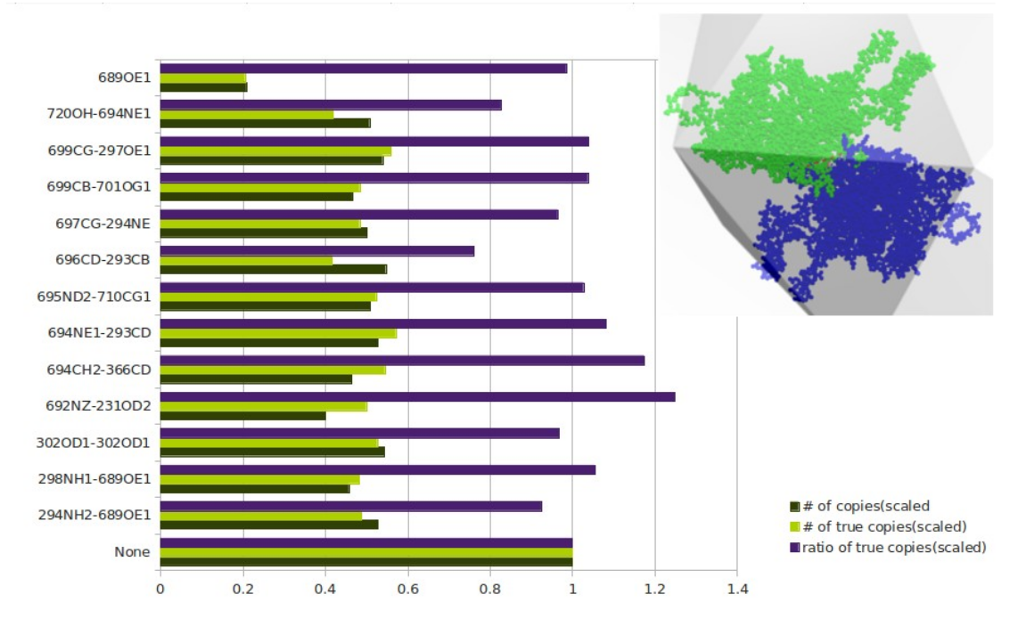
Figure 11: Assembly of a dimer, 2-fold interface of the icosahedral AAV2 virus capsid. Each row corresponds to removing a particular residue pair. These are normalized to the bottom row where no interaction is removed and shows respectively the total number of zero-dimensional (rigid) configurations, the number of configurations close to the successful interface assembly configuration, and their ratio. [60].

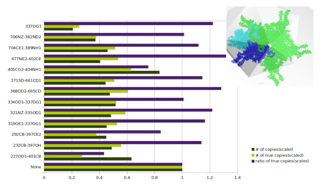
Figure 12: Assembly of a pentamer, 5-fold interface of the icosahedral AAV2 virus capsid. Each row corresponds to removing a particular residue pair. These are normalized to the bottom row when no interaction is removed and shows respectively the total number of zero-dimensional or rigid configurations, the number of configurations close to the successful interface assembly configuration, and their ratio. [60].

In this section we sketch results from [60]. EASAL has been applied to study the configuration space of autonomous assembly into empty shells of icosahedral T=1 viruses from nearly identical protein monomers containing $n\geq 5000$ atoms. The robustness of such an assembly depends on the sensitivity of free energy landscapes of inter-monomer interfaces to changes in the governing inter-atomic interactions. The sensitivity towards assembly disruption is generally measured by wet lab mutagenesis that disables the chosen inter-monomer atomic interactions. [60] predicted this sensitivity for the first time using EASAL to atlas the inter-monomer interface configuration space, exploiting symmetries, and utilizing the recursive decomposition of the large viral capsid assembly into an assembly pathway of smaller assembly intermediates. The predictions were compared with the results from the mutagenesis. Specifically, EASAL was used to predict the sensitivity of 3 viral systems: Minute Virus of Mice (MVM), Adeno-Associated Virus (AAV2), and Bromo-Mosaic Virus (BMV). For the case of AAV2, Fig. 11 and Fig. 12 show the effect of removing a particular residue pair (the BMV results are not shown here, [58]). Each row shows the total number of zero-dimensional or rigid configurations, the number of configurations close to the successful interface assembly configuration, and their ratio. Table 4 shows comparison of the cruciality or sensitivity ranking thereby obtained to the mutagenesis result. The highest ranked interactions output by EASAL were validated by mutagenesis resulting in assembly disruption. The sensitivity ranking of the dimer interface shows that all the residues marked crucial by EASAL were confirmed as crucial by wet lab mutagenesis. The entries not listed in the table, corresponding to non-crucial interactions, were either confirmed as not crucial or there were no experiments performed for them. The sensitivity ranking for the pentamer shows similar results, however experiments for some of the residues marked by a question mark were not performed.

Residue1	Residue2	Confirmed
P293	W694, P696	Yes∗,†
R294	E689, E697	Yes ∗,†,∗∗
E689	R298	Yes ∗,†
W694	P293, Y397	Yes ∗,†
P696	P293	Yes ∗,†
Y720	W694	Yes ∗,†

Sensitivity ranking: Dimer Interface

Residue1	Residue2	Confirmed
N227	Q401	Yes ∗∗
R389	Y704	?
K706	N382	?
M402	Q677	Yes ∗,†
K706	N382	?
N334	T337,Q319	?
S292	F397	Yes ∗∗

Sensitivity ranking: Pentamer Interface

Table 4: Sensitivity ranking for the dimer and pentamer interface of AAV2. For some residue pairs, marked by ‘?’, there were no experiments performed and their cruciality is unconfirmed. ^∗ - [50], ^† - [6], ^∗∗ - [46]

5 Software architecture

The EASAL software has two versions. The TOMS submission contains only the backend of EASAL, without GUI and with text input and output. An optional GUI (not part of TOMS submission) which can be used for intuitive visual verification of the results, can be found at the EASAL bitbucket repository [43]. Fig. 13, which shows the overall architecture of EASAL, clearly demarcates these two versions.

The user initiates the sampling either by running just the backend in a terminal or through the optional GUI (not part of TOMS submission). The AtlasBuilder starts the sampling process by making a recursive call to the ‘sampleAtlasNode’ algorithm with the root node as the parameter. The Atlas builder interacts with various components such as ‘Cayley parameterization’, ‘Cartesian Realization’ and ‘Constraint Check’ to help in the sampling process. It uses the ‘SaveLoader’ to save the generated atlas to the database. All the sampling information such as the atlas, active constraint graphs, Cayley parameters and realizations are written to a database to avoid re-sampling.

When EASAL is initiated using the backend, the output is in text format. The following are the output:

• The Roadmap, which stores the atlas, i.e., a topologically stratified set of sample feasible realizations or configurations of the two rigid point sets. This can be found in the ‘RoadMap.txt’ file in the data folder.

• The Node files which contain sampling information, Cayley parameter values, and realizations of the point sets. Each ‘Node*.txt’ file contains samples for a particular active constraint region.

• The paths file which contains the one degree of freedom motion path between all pairs of lowest energy configuration regions. This can be found in the ‘paths.txt’ file in the data folder.

• The path matrix, which contains a path matrix where the rows and columns correspond to 0D and 1D nodes. The $\{ij\}^{th}$ entry indicates the number of paths between nodes $i$ and $j$. This can be found in the ‘path_matrix.txt’ file in the data folder.

The optional GUI (not part of TOMS submission) can be used to visualize the output of the backend. See Section 3.3.5 of the ‘Complete User Guide’ located in the bitbucket repository [43] for instructions. The optional GUI has three views: the atlas view, the Cayley space view and the realization view. The atlas view shows the stratification of the configuration space in the form of an atlas. In the atlas view, the user can explore the atlas by intervening in the sampling process to either complete, redirect, refine or limit the sampling. The user can also propose new constraints for active constraint graphs. The Cayley space view shows the user the Cayley configuration space of a node in the atlas. In the Cayley space view the user can view all the Cayley parameters and boundaries. In the realization view, the user can view all the Cartesian realizations of the selected node. This view contains the sweep feature which keeps one of the point-sets fixed and draws the other point-set many times to trace out the set of all feasible realizations.

Figure 13: Architecture of EASAL.

6 Conclusion

The EASAL software generates, describes, and explores key aspects of the topology and geometry of the configuration space of point-sets in $\mathbb{R}^{3}$. To achieve this, it uses three strategies, (i) EASAL partitions the realization space into active constraint regions each defined by the set of active constraints. The graph of active constraints called the active constraint graph is then used for analysis using generic combinatorial rigidity theory. (ii) EASAL organizes the active constraint regions in a partial order called an atlas which establishes a parent child relationship between active constraint regions that generically differ by exactly one active constraint. To build the atlas, EASAL starts from the interior of an active constraint region and recursively finds boundaries of one dimension less. (iii) To locate the boundary region satisfying exactly one additional constraint, EASAL uses the theory of Cayley convexifiability to map (many to one) a $d$-dimensional active constraint region to a convex region in $\mathbb{R}^{d}$ called the Cayley configuration space of the region. This allows for efficient sampling and search. In addition, it is efficient to compute the inverse map from each point in the Cayley configuration space to its finitely many Cartesian realizations. With EASAL we obtain formal guarantees for quantitative accuracy and running times. The EASAL software optionally provides a GUI which can be used for intuitive visual verification of results.

In the context of molecular assembly, EASAL distinguishes assembly from other processes such as folding in that assembly admits to Cayley convexification of active constraint regions. More general methods like MC and MD, though applicable to a wider variety of molecular modeling problems, do not make this distinction and hence are not as efficient as EASAL in the context of molecular assembly. For the problem of assembly, EASAL (i) directly atlases and navigates the complex topology of small assembly configuration spaces, crucial for understanding free-energy landscapes and assembly kinetics; (ii) avoids multiple sampling of configurational (boundary) regions, and minimizes rejected samples, both crucial for efficient and accurate computation of configurational volume and entropy and (iii) comes with rigorously provable efficiency, accuracy and tradeoff guarantees. To the best of our knowledge, no other current software provides such functionality.

The paper reviews the key theoretical underpinnings, major algorithms and their implementation; outlines the main applications such as computation of free energy and kinetics of assembly of supramolecular structures or of clusters in colloidal and soft materials; and surveys select experimental results and comparisons.

References

- [1] Ioan Andricioaei and Martin Karplus. On the calculation of entropy from covariance matrices of the atomic fluctuations. The Journal of Chemical Physics, 115(14):6289, 2001.
- [2] Natalie Arkus, Vinothan Manoharan, and Michael Brenner. Minimal Energy Clusters of Hard Spheres with Short Range Attractions. Physical Review Letters, 103(11):118303, September 2009.
- [3] Yuliy Baryshnikov, Peter Bubenik, and Matthew Kahle. Min-type morse theory for configuration spaces of hard spheres. International Mathematics Research Notices, 2014(9):2577, 2014.
- [4] Saugata Basu, Richard Pollack, and Marie-Françoise Roy. Computing roadmaps of semi-algebraic sets on a variety. Journal of the American Mathematical Society, 13:55–82, 2000.
- [5] Daniel J. Beltran-Villegas and Michael A. Bevan. Free energy landscapes for colloidal crystal assembly. Soft Matter, 7(7):3280–3285, 2011.
- [6] Antonette Bennett. 2012. Unpublished manuscript.
- [7] Sergei Bespamyatnikh, Vicky Choi, Herbert Edelsbrunner, and Johannes Rudolph. Accurate protein docking by shape complementarity alone. Manuscript, Duke Univ., Durham, NC, 2004.
- [8] Peter Bubenik, Gunnar Carlsson, Peter T Kim, and Zhi-Ming Luo. Statistical topology via morse theory persistence and nonparametric estimation. Algebraic methods in statistics and probability II, 516:75–92, 2010.
- [9] Florent Calvo, Jonathan P K Doye, and David J Wales. Energy landscapes of colloidal clusters: thermodynamics and rearrangement mechanisms. Nanoscale, 4(4):1085–100, February 2012.
- [10] J. Canny. A new algebraic method for robot motion planning and real geometry. In 28th Annual Symposium on Foundations of Computer Science (sfcs 1987), pages 39–48, Oct 1987.
- [11] John Canny. Computing roadmaps of general semi-algebraic sets. Computer Journal, 36:504–514, 1993.
- [12] Gunnar Carlsson, Jackson Gorham, Matthew Kahle, and Jeremy Mason. Computational topology for configuration spaces of hard disks. Phys. Rev. E, 85:011303, Jan 2012.
- [13] Gregory S. Chirikjian. Chapter four – modeling loop entropy. In Michael L. Johnson and Ludwig Brand, editors, Computer Methods Part C, volume 487 of Methods in Enzymology, pages 99 – 132. Academic Press, 2011.
- [14] Ugandhar Reddy Chittamuru. Efficient bounds for 3D Cayley configuration space of partial 2-trees. Master’s thesis, University of Florida, 2010.
- [15] Vicky Choi, Pankaj K Agarwal, Herbert Edelsbrunner, and Johannes Rudolph. Local search heuristic for rigid protein docking. In International Workshop on Algorithms in Bioinformatics, pages 218–229. Springer, 2004.
- [16] Aleksandar Donev, Salvatore Torquato, Frank H. Stillinger, and Robert Connelly. Jamming in hard sphere and disk packings. Journal of Applied Physics, 95(3), 2004.
- [17] Dina Duhovny, Ruth Nussinov, and Haim J. Wolfson. Efficient Unbound Docking of Rigid Molecules, pages 185–200. Springer Berlin Heidelberg, Berlin, Heidelberg, 2002.
- [18] David Gfeller, David Morton De Lachapelle, Paolo De Los Rios, Guido Caldarelli, and Francesco Rao. Uncovering the topology of configuration space networks. Physical Review E - Statistical, Nonlinear and Soft Matter Physics, 76(2 Pt 2):026113, 2007.
- [19] Jack Graver, Brigitte Servatius, and Herman Servatius. Combinatorial Rigidity Graduate Studies in Mathematics, volume 2. American Mathematical Society, 1993.
- [20] Martha S Head, James A Given, and Michael K Gilson. Mining minima: Direct computation of conformational free energy. The Journal of Physical Chemistry A, 101(8):1609–1618, 1997.
- [21] Ulf Hensen, Oliver F Lange, and Helmut Grubmüller. Estimating absolute configurational entropies of macromolecules: The minimally coupled subspace approach. PLoS ONE, 5(2):8, 2010.
- [22] Vladimir Hnizdo, Eva Darian, Adam Fedorowicz, Eugene Demchuk, Shengqiao Li, and Harshinder Singh. Nearest-neighbor nonparametric method for estimating the configurational entropy of complex molecules. Journal of Computational Chemistry, 28(3):655–668, 2007.
- [23] Vladimir Hnizdo, Jun Tan, Benjamin J Killian, and Michael K Gilson. Efficient calculation of configurational entropy from molecular simulations by combining the mutual-information expansion and nearest-neighbor methods. Journal of Computational Chemistry, 29(10):1605–1614, 2008.
- [24] Miranda Holmes-Cerfon, Steven J Gortler, and Michael P Brenner. A geometrical approach to computing free-energy landscapes from short-ranged potentials. Proceedings of the National Academy of Sciences of the United States of America, 110(1):E5–14, January 2013.
- [25] Robert S. Hoy. Structure and dynamics of model colloidal clusters with short-range attractions. July 2014.
- [26] Robert S. Hoy, Jared Harwayne-Gidansky, and Corey S. O’Hern. Structure of finite sphere packings via exact enumeration: Implications for colloidal crystal nucleation. Physical Review E, 85(5):051403, May 2012.
- [27] Léonard Jaillet and Josep Maria Porta. Path planning with loop closure constraints using an atlas-based RRT. In International Symposium on Robotics Research (ISRR), 2011.
- [28] J. E. Jones. On the determination of molecular fields. ii. from the equation of state of a gas. Proceedings of the Royal Society of London A: Mathematical, Physical and Engineering Sciences, 106(738):463–477, 1924.
- [29] Matthew Kahle. Random geometric complexes. Discrete & Computational Geometry, 45(3):553–573, 2011.
- [30] Matthew Kahle. Sparse locally-jammed disk packings. Annals of Combinatorics, 16(4):773–780, 2012.
- [31] M. Karplus and J.N. Kushick. Method for estimating the configurational entropy of macromolecules. Macromolecules, 14(2):325–332, 1981.
- [32] E. Katchalski-Katzir, I. Shariv, M. Eisenstein, A. A. Friesem, C. Aflalo, and I. A. Vakser. Molecular surface recognition: determination of geometric fit between proteins and their ligands by correlation techniques. Proc. Natl. Acad. Sci. U.S.A., 89(6):2195–2199, Mar 1992.
- [33] L. E. Kavraki, M. N. Kolountzakis, and J. C. Latombe. Analysis of probabilistic roadmaps for path planning. IEEE Transactions on Robotics and Automation, 14(1):166–171, Feb 1998.
- [34] L. E. Kavraki, P. Svestka, J. C. Latombe, and M. H. Overmars. Probabilistic roadmaps for path planning in high-dimensional configuration spaces. IEEE Transactions on Robotics and Automation, 12(4):566–580, Aug 1996.
- [35] Siddique J Khan, O L Weaver, C M Sorensen, and A Chakrabarti. Nucleation in short-range attractive colloids: ordering and symmetry of clusters. Langmuir : the ACS journal of surfaces and colloids, 28(46):16015–21, November 2012.
- [36] Benjamin J Killian, Joslyn Yundenfreund Kravitz, and Michael K Gilson. Extraction of configurational entropy from molecular simulations via an expansion approximation. The Journal of chemical physics, 127(2):024107, 2007.
- [37] Bracken M. King, Nathaniel W. Silver, and Bruce Tidor. Efficient calculation of molecular configurational entropies using an information theoretic approximation. The Journal of Physical Chemistry B, 116(9):2891–2904, 2012. PMID: 22229789.
- [38] Tzee-Char Kuo. On thom-whitney stratification theory. Mathematische Annalen, 234:97–107, 1978. 10.1007/BF01420960.
- [39] Zaizhi Lai, Jiguo Su, Weizu Chen, and Cunxin Wang. Uncovering the properties of energy-weighted conformation space networks with a hydrophobic-hydrophilic model. International Journal of Molecular Sciences, 10(4):1808–1823, 2009.
- [40] Shawn Martin, Aidan Thompson, Evangelos A Coutsias, and Jean-Paul Watson. Topology of cyclo-octane energy landscape. The Journal of chemical physics, 132(23):234115, June 2010.
- [41] James Clerk Maxwell. On reciprocal figures and diagrams of forces. Philosophical Magazine, 27:250–261, 1864.
- [42] Aysegul Ozkan, JC Flores-Canales, Maria Kurnikova, and Meera Sitharam. Geometrical algorithm for enhanced sampling of compact configurations in protein docking problem. (on arxiv, manuscript under review), 2014.
- [43] Aysegul Ozkan, Rahul Prabhu, Troy Baker, James Pence, and Meera Sitharam. Efficient atlasing and search of assembly landscapes (ACM TOMS version), 2016.
- [44] Aysegul Ozkan and Meera Sitharam. EASAL: Efficient atlasing, analysis and search of molecular assembly landscapes. In Proceedings of the ISCA 3rd International Conference on Bioinformatics and Computational Biology, BICoB-2011, 2011.
- [45] Aysegul Ozkan and Meera Sitharam. Best of both worlds: Uniform sampling in Cartesian and Cayley molecular assembly configuration space. (on arxiv, manuscript under review), 2014.
- [46] Wu P., T. Conlon, J. Hughes, M. Agbandje-McKenna, T. Ferkol, T. Flotte, and N. Muzyczka. Mutational analysis of the adeno-associated virus type 2 (aav2) capsid gene and construction of aav2 vectors with altered tropism. Virol, 74:8635–86, 2000.
- [47] Josep M Porta, Lluís Ros, Federico Thomas, Francesc Corcho, Josep Cantó, and Juan Jesús Pérez. Complete maps of molecular-loop conformational spaces. Journal of computational chemistry, 28(13):2170–89, October 2007.
- [48] Rahul Prabhu, Troy Baker, and Meera Sitharam. Video illustrating the version of open source EASAL submitted to ACM TOMS, 2016.
- [49] Diego Prada-Gracia, Jes s G mez-Garde es, Pablo Echenique, and Fernando Falo. Exploring the free energy landscape: From dynamics to networks and back. PLoS Comput Biol, 5(6):e1000415, 06 2009.
- [50] Vamseedhar Rayaprolu, Shannon Kruse, Ravi Kant, Balasubramanian Venkatakrishnan, Navid Movahed, Dewey Brooke, Bridget Lins, Antonette Bennett, Timothy Potter, Robert McKenna, Mavis Agbandje-McKenna, and Brian Bothner. Comparative analysis of adeno-associated virus capsid stability and dynamics. Journal of Virology, 87(24):13150–13160, 2013.
- [51] D. Schneidman-Duhovny, Y. Inbar, R. Nussinov, and H. J. Wolfson. PatchDock and SymmDock: servers for rigid and symmetric docking. Nucleic Acids Res., 33(Web Server issue):W363–367, Jul 2005.
- [52] Meera Sitharam and Heping Gao. Characterizing graphs with convex and connected cayley configuration spaces. Discrete & Computational Geometry, 43(3):594–625, 2010.
- [53] Meera Sitharam, Aysegul Ozkan, and Ruijin Wu. Efficient atlasing and sampling of assembly free energy landscapes using EASAL: Stratification and convexification via customized Cayley parametrization. (on arxiv, manuscript under review), 2014.
- [54] Meera Sitharam, Andrew Vince, Menghan Wang, and Miklós Bóna. Symmetry in sphere-based assembly configuration spaces. Symmetry, 8(1):5, 2016.
- [55] G Varadhan, Y J Kim, S Krishnan, and D Manocha. Topology preserving approximation of free configuration space. Robotics, (May):3041–3048, 2006.
- [56] David J Wales. Energy landscapes of clusters bound by short-ranged potentials. Chemphyschem : a European journal of chemical physics and physical chemistry, 11(12):2491–4, August 2010.
- [57] Wikipedia. Molecular self-assembly, accessed Dec 2017.
- [58] Ruijin Wu, Antonette Bennet, Mavis Agbandje-Mckenna, and Meera Sitharam. Detecting assembly crucial interactions for viral capsid assembly using configuration space atlasing. 2015. In preparation.
- [59] Ruijin Wu, Aysegul Ozkan, Antonette Bennett, Mavis Agbandje-Mckenna, and Meera Sitharam. Robustness measure for an adeno-associated viral shell self-assembly is accurately predicted by configuration space atlasing using EASAL. In Proceedings of the ACM Conference on Bioinformatics, Computational Biology and Biomedicine, BCB ’12, pages 690–695, New York, NY, USA, 2012. ACM.
- [60] Ruijin Wu, Aysegul Ozkan, Antonette Bennett, Mavis Agbandje-Mckenna, and Meera Sitharam. Robustness measure for an adeno-associated viral shell self-assembly is accurately predicted by configuration space atlasing using easal. In Proceedings of the ACM Conference on Bioinformatics, Computational Biology and Biomedicine, BCB ’12, pages 690–695, New York, NY, USA, 2012. ACM.
- [61] Yuan Yao, Jian Sun, Xuhui Huang, Gregory R Bowman, Gurjeet Singh, Michael Lesnick, Leonidas J Guibas, Vijay S Pande, and Gunnar Carlsson. Topological methods for exploring low-density states in biomolecular folding pathways. The Journal of chemical physics, 130(14):144115, 2009.