TUM-HEP-1139/18
arXiv:1805.07367
May 01, 2020

Energetic $\gamma$-rays from TeV scale dark matter
annihilation resummed

M. Beneke^a, A. Broggio^a, C. Hasner^a,

and M. Vollmann^a
aPhysik Department T31,
James-Franck-Straße 1, Technische Universität München,
D–85748 Garching, Germany

The annihilation cross section of TeV scale dark matter particles $\chi^{0}$ with electroweak charges into photons is affected by large quantum corrections due to Sudakov logarithms and the Sommerfeld effect. We calculate the semi-inclusive photon energy spectrum in $\chi^{0}\chi^{0}\to\gamma+X$ in the vicinity of the maximal photon energy $E_{\gamma}=m_{\chi}$ with NLL’ accuracy in an all-order summation of the electroweak perturbative expansion adopting the pure wino model. This results in the most precise theoretical prediction of the annihilation rate for $\gamma$-ray telescopes with photon energy resolution of parametric order $m_{W}^{2}/m_{\chi}$ for photons with TeV energies.

1 Introduction

Within the large variety of dark matter (DM) candidates a weakly interacting particle with mass $m_{\chi}$ in the 100 GeV to 10 TeV range (WIMP) stands out due to its conceptual minimality and its relation to the electroweak scale. Although loop suppressed, the pair annihilation of WIMPs into two photons or a photon and a $Z$ boson often provides a distinctive signature in the form of a monochromatic component of high-energy cosmic $\gamma$-rays. The strongest limit on such $\gamma$-line signals is currently set by the H.E.S.S. experiment [1]. This limit is expected to be improved by an order of magnitude by the Cherenkov Telescope Array (CTA) [2] under construction, which will severely constrain generic WIMP models. This motivates a thorough theoretical investigation of the basic pair annihilation cross section given a particular model.

It is well-known that TeV-scale DM annihilation is not accurately described by the leading-order annihilation rate, but is modified by the Sommerfeld effect [3] generated by the electroweak Yukawa force on the DM particles prior to their annihilation. In terms of Feynman diagrams the Sommerfeld effect corresponds to ladder diagrams with $W$, $Z$, photon and Higgs boson exchange, which contribute ${\cal O}((m_{\chi}\alpha_{2}/m_{W})^{n})$ at order $n$, where $m_{W}$ is the $W$ boson mass and $\alpha_{2}$ the SU(2) gauge coupling. For annihilation rates to exclusive final states, in addition to the Sommerfeld effect large logarithmically enhanced quantum corrections of ${\cal O}((\alpha_{2}\ln^{2}(m_{\chi}/m_{W}))^{n})$, also known as electroweak Sudakov logarithms, arise [4] from the restriction on the emission of soft radiation. Electroweak Sudakov logarithms in DM annihilation into photons have been identified as a potential source of large corrections and resummed to all orders in perturbation theory in previous work [5, 6, 7, 8, 9] in models with an electroweak triplet scalar or fermionic DM particle.

In this letter we revisit this question starting from the observation that telescopes do not measure two photons from a single decay in coincidence. Rather, the observable is the semi-inclusive single-photon energy spectrum $\gamma+X$, where $X$ denotes the unidentified other final state particles. This spectrum is composed of two spectral line features related to the $\gamma\gamma$ and $\gamma Z$ final states and a continuum from multi-body final states. While the leading term in the expansion in $\alpha_{2}$ is indeed exclusively from the $\gamma\gamma$ and $\gamma Z$ final state, the logarithmically enhanced quantum corrections are different for the exclusive and the semi-inclusive measurement. If $E^{\gamma}_{\rm res}\ll m_{\chi}$ denotes the energy resolution of the instrument for photon energies $E_{\gamma}\approx m_{\chi}$, the maximal invariant mass of the unobserved final state $X$ is $m_{X}^{2}=4m_{\chi}E^{\gamma}_{\rm res}\ll m_{\chi}^{2}$. Since $X$ must balance the large momentum of the observed photon, $X$ is forced to have a ‘jet-like’ structure. The kinematic situation involving non-relativistic heavy particles in the initial state and energetic, small-invariant mass objects in the final state is naturally described by a combination of non-relativistic and soft-collinear effective field theory, similar to the QCD treatment of the ‘inverse’ situation of hadronic production of two heavy particles [10].

In the following sections we first summarize briefly the basic elements of an effective field theory (EFT) treatment of the single-inclusive photon spectrum $d(\sigma v)/dE_{\gamma}$ in DM pair annihilation near the kinematic endpoint. For the DM model we refer to the widely discussed pure wino model, which features an electroweak triplet whose electrically neutral component is the DM particle, although all results except the one for the soft function and the Sommerfeld factor apply more generally to DM particles in an arbitrary isospin-$j$ multiplet. We then present and discuss our result for the all-order resummed spectrum including both the Sommerfeld and Sudakov corrections. A more detailed exposition of the formalism as well as extensions will be reported in a longer article. While this work was being finalized, a similar EFT calculation of the endpoint of the $\gamma+X$ spectrum has appeared [11]. The present EFT formulation refers to a finer photon energy resolution, but includes the one-loop corrections to all matching coefficients, soft and jet functions thus achieving NLL’ rather than LL accuracy for the observable in question.

2 The resummed energy spectrum

We add to the Standard Model (SM) Lagrangian a fermionic multiplet $\chi$ (which can be of Majorana or Dirac type) in an arbitrary isospin-$j$ representation of the electroweak (EW) SU(2) gauge group. For the Majorana case, only integer $j$ are allowed, while for the Dirac case also half-integer $j$ are possible. In the calculations below we assume zero hypercharge ($Y=0$), in which case only integer $j$ multiplets provide a realistic DM particle as the electrically neutral member $\chi^{0}$ of the $2j+1$ dimensional multiplet. The Lagrangian is

$$\mathcal{L}=\mathcal{L}_{\text{SM}}+\overline{\chi}(i\not{D}-m_{\chi})\chi$$ (1)

when $\chi$ is a Dirac fermion. For the Majorana case, $\chi$ is self-conjugate and its Lagrangian is multiplied by $1/2$. The SU(2) covariant derivative is $D_{\mu}=\partial_{\mu}-ig_{2}A^{C}_{\mu}\,T^{C}$ where $T^{C}$, $C=1,2,3$, are the SU(2) generators in the isospin-$j$ representation and $A_{\mu}^{C}$ are the EW gauge bosons. In these models the dark matter particle obtains the correct relic density from thermal freeze-out for $m_{\chi}$ in the 1-10 TeV range [12] for the favoured small representations $j=1,2$.

2.1 Effective theory framework

We consider the process

$$\chi^{0}(p_{1})+\chi^{0}(p_{2})\to\gamma(p_{\gamma})+X(p_{X})$$ (2)

for nearly maximal photon energy. Since the kinetic energy of the dark matter particles is negligible, $E^{\gamma}_{\rm max}=m_{\chi}$. The theoretically calculated energy spectrum is distribution-valued. We integrate the energy spectrum over an interval $E^{\gamma}_{\rm res}$ from the endpoint,

$$\langle\sigma v\rangle(E^{\gamma}_{\rm res})=\int_{m_{\chi}-E^{\gamma}_{\rm res}}^{m_{\chi}}dE_{\gamma}\,\frac{d(\sigma v)}{dE_{\gamma}}\,.$$ (3)

Roughly speaking, for a $\gamma$-telescope with resolution $E^{\gamma}_{\rm res}$, this together with the astrophysical line-of-sight factor determines the flux of photons from dark matter annihilation into the energy bin that contains the photon line signal. To turn experimental limits into model constraints, requires to replace the above integral by an integral with the experiment-specific response function. Eq. (3) is useful to quantify the importance of radiative corrections and resummation for the semi-inclusive energy spectrum from dark matter annihilation for $E_{\gamma}$ near $m_{\chi}$, and will be used below.

The photon endpoint spectrum depends on four important scales: $m_{\chi}$ (hard), the small invariant mass $m_{X}=\sqrt{4m_{\chi}E^{\gamma}_{\rm res}}$ (collinear) of the unobserved, energetic final state, enforced by the kinematics of the endpoint, the electroweak scale $m_{W}$ (soft) and the energy resolution scale $E^{\gamma}_{\rm res}$ (ultrasoft). We shall now assume that the energy resolution is parametrically of order $E^{\gamma}_{\rm res}\sim m_{W}^{2}/m_{\chi}$, which implies $m_{X}\sim m_{W}$ and the scale hierarchy $E^{\gamma}_{\rm res}\ll m_{W},m_{X}\ll m_{\chi}$. The factorization of the multi-scale Feynman diagrams into single-scale contributions, which is a prerequisite to all-order resummation, then requires the introduction of momentum modes with the following parametric scaling:

$$\text{hard}\,(h):\quad k^{\mu}\sim m_{\chi}(1,1,1)$$

$$\text{collinear}\,(c):\quad k^{\mu}\sim m_{\chi}(1,\lambda^{2},\lambda)$$

$$\text{anti-collinear}\,(\bar{c}):\quad k^{\mu}\sim m_{\chi}(\lambda^{2},1,\lambda)$$

$$\text{soft}\,(s):\quad k^{\mu}\sim m_{\chi}(\lambda,\lambda,\lambda)$$ (4)

$$\text{potential}\,(p):\quad k^{0}\sim m^{2}_{W}/m_{\chi},\,\mathbf{k}\sim m_{W}$$

$$\text{ultrasoft}\,(s):\quad k^{\mu}\sim m_{\chi}(\lambda^{2},\lambda^{2},\lambda^{2})$$

Here $\lambda=\sqrt{E^{\gamma}_{\rm res}/m_{\chi}}$ and $k^{\mu}\sim(n_{+}\cdot k,n_{-}\cdot k,\,\mathbf{k}_{\perp})$ where $n_{+}^{\mu},n_{-}^{\mu}$ are two light-like vectors with $p_{\gamma}^{\mu}=E_{\gamma}n_{+}^{\mu}$ and $n_{+}\cdot n_{-}=2$. We remark that the collinear, anti-collinear, soft and potential modes all have the same virtuality ${\cal O}(m_{W}^{2})$. The interactions of these modes are described by standard potential non-relativistic and soft-collinear effective Lagrangians (similar to [10], generalized from QCD to the electroweak interaction).

The energy resolution of existing instruments is considerably larger than assumed here. For $m_{\chi}=3\,$TeV, allowing for $E_{\rm res}^{\gamma}\sim 4m_{W}^{2}/m_{\chi}$ amounts to a resolution of about 10 GeV or $0.3\%$ compared to 10% of, for example, H.E.S.S. One might also consider the wider resolution $E^{\gamma}_{\rm res}\sim m_{W}$, which implies $E^{\gamma}_{\rm res},m_{W}\ll m_{X}\ll m_{\chi}$ and a different mode structure. Conceptually, the main difference is caused by the fact that the previous, narrower resolution does not allow the radiation of soft particles with electroweak-scale masses into the unobserved final state. Although the resolution of the up-coming $\gamma$-ray telescopes is probably closer to the wide resolution case, in this work we concentrate on the narrow resolution $E^{\gamma}_{\rm res}\sim m_{W}^{2}/m_{\chi}$ to stay close to the line-like signal. The wide resolution case, which is in fact simpler from the EFT point of view, will be discussed in subsequent work, which will also provide the explicit forms of the effective Lagrangians.

2.2 Factorization

The primary annihilation process is described at leading order in an expansion in $\lambda$, which is also an expansion in $m_{W}/m_{\chi}$, by operators ${\cal O}_{i}$ for the S-wave annihilation of the dark matter particles into two EW gauge bosons. Once the hard modes are integrated out into the coefficient functions $C_{i}$ of these operators, the collinear, anti-collinear and potential fields can no longer interact directly, since their momenta would add up to hard virtualities. The collinear modes build up the unobserved final state $X$, while the anti-collinear modes must result in the single, observed photon. The non-relativistic DM particles are described by the potential fields exchanging potential EW gauge bosons, which causes the Sommerfeld effect.

The factorization formula then follows from an analysis of the coupling of the (ultra) soft modes to any of the above. The decoupling of soft gauge boson attachments from heavy-particle fields in the presence of the Sommerfeld effect by a time-like Wilson-line field redefinition of the heavy-particle field has been demonstrated in [10] for an unbroken gauge theory. Although in the present case the Sommerfeld effect must be computed in the broken theory with gauge boson masses, soft attachments still factorize from the ladder diagrams, since a soft momentum throws the potential heavy particle off-shell, which removes the enhancement of the ladder rungs between the soft attachment and the hard vertex. It follows that the Sommerfeld factor $S_{IJ}$ completely factorizes from the Sudakov resummed annihilation rate $\Gamma_{IJ}(E_{\gamma})$,

$$\frac{d(\sigma v_{\text{rel}})}{dE_{\gamma}}=2\sum_{I,J}S_{IJ}\,\Gamma_{IJ}(E_{\gamma})\,,$$ (5)

where the sums over $I,J$ run over all electrically neutral two-particle states that can be formed from the $2j+1$ single-particle states of the electroweak DM multiplet. For example, in the triplet (‘wino’) model, $I,J=\chi^{0}\chi^{0},\chi^{+}\chi^{-}$. Since gauge boson exchange between the DM particles prior to annihilation can change the initial two-particle state $\chi^{0}\chi^{0}$ into any $I,J$, the annihilation rate with the Sommerfeld effect factored out is a matrix describing the amplitude for the annihilation of two-particle state $I$ times the complex conjugate of the annihilation amplitude for state $J$. The Sommerfeld factor is defined in terms of the matrix element of non-relativistic DM fields of the schematic form $\langle\chi^{0}\chi^{0}|[\chi\chi]_{J}|0\rangle\langle 0|[\chi\chi]_{I}|\chi^{0}\chi^{0}\rangle$ such that $S_{IJ}=\delta_{IJ}$ in the absence of the potential force causing the Sommerfeld effect (see [13] for the full definitions).

The coupling of soft gauge fields to collinear and anti-collinear fields is removed by a redefinition of the (anti) collinear fields with light-like Wilson lines [14]. Since the small energy resolution forbids soft radiation into the final state $X$, the soft function is a vacuum matrix element of Wilson lines that can be regarded as a soft Wilson coefficient $D$ of the annihilation amplitude [15, 16] on top of the hard Wilson coefficients $C_{i}$ of the operators ${\cal O}_{i}$. At this point all modes have been factored into separate functions except for the coupling of ultrasoft fields. At leading order in the expansion in $\lambda$, the coupling of ultrasoft gauge fields is again described by Wilson lines, where now the gauge field must be the photon. Since the initial state is electrically neutral and at rest, the coupling of ultrasoft photons is of higher-order, leaving ultrasoft Wilson lines from the (anti) collinear fields. There is no kinematic restriction on the radiation of ultrasoft particles with energy and masses of order $E_{\gamma}^{\rm res}$ into the final state, hence the ultrasoft function corresponds to an amplitude squared summed over the unobserved ultrasoft final state.

We can therefore write down the following factorization formula for the energy spectrum of DM annihilation (more precisely, the off-diagonal annihilation matrix $\Gamma_{IJ}$ in the DM two-particle states) into a single identified-photon inclusive final state near the maximal photon energy:

$$\Gamma_{IJ}(E_{\gamma}) = \frac{1}{(\sqrt{2})^{n_{id}}}\,\frac{1}{4}\,\frac{2}{\pi m_{\chi}}\sum_{i,j\,=\,1,2}\,\sum_{V,W,X,Y}C^{*}_{j}(\mu_{W})C_{i}(\mu_{W})D_{J,XY}^{j\,*}(\mu_{W},\nu_{s})D_{I,VW}^{i}(\mu_{W},\nu_{s})$$ (6)

$$\times\,V(\mu_{W},\nu_{s},\nu_{j})\,Z_{\gamma}^{YW}\,\int d\omega\,J^{XV}(4m_{\chi}(m_{\chi}-E_{\gamma}-\omega),\mu_{W},\nu_{j})\,S_{\gamma}(\omega)$$

The prefactors account for the spin average, flux factor and photon momentum angular integration, $C$ and $D$ refer to the hard and soft matching coefficients of the annihilation amplitude. The former is evolved from the scale $2m_{\chi}$ to the electroweak scale $\mu_{W}$. The indices $V,W,X,Y$ refer to the SU(2) adjoint representation of the electroweak gauge bosons. In the second line $Z_{\gamma}$ is the anti-collinear factor for the observed photon, $J$ the jet function for the unobserved collinear final state $X$, convoluted with the ultrasoft function $S$. Since the (anti) collinear and soft modes have parametrically equal virtualities, a rapidity evolution factor $V(\mu_{W},\nu_{s},\nu_{j})$ is needed. We postpone the derivation of this formula and technical details to a separate paper and proceed by defining the appearing functions and providing the results of their calculation.

2.2.1 Operator basis and hard matching coefficients

The relevant hard annihilation operators can be written as

$$\mathcal{O}_{1} = \chi_{v}^{c\dagger}\Gamma^{\mu\nu}\chi_{v}\,\mathcal{A}^{B}_{\perp c,\mu}(sn_{+})\mathcal{A}^{B}_{\perp\bar{c},\nu}(tn_{-})\,,$$ (7)

$$\mathcal{O}_{2} = \frac{1}{2}\,\chi_{v}^{c\dagger}\Gamma^{\mu\nu}\{T^{B},T^{C}\}\chi_{v}\,\mathcal{A}^{B}_{\perp c,\mu}(sn_{+})\mathcal{A}^{C}_{\perp\bar{c},\nu}(tn_{-})\,.$$ (8)

Here $\chi_{v}$ is a two-component non-relativistic spinor field in the SU(2) weak isospin $j$ representation, $\chi_{v}^{c}=-i\sigma^{2}\chi_{v}^{*}$ the charge-conjugated field, and $\mathcal{A}^{B}_{\perp c,\mu}$ the collinear gauge-invariant collinear gauge field of soft-collinear effective theory (SCET). Collinear fields have large momentum component $n_{+}p$. A similar definition applies to the anti-collinear direction with $n_{+}$ and $n_{-}$ interchanged. Fields without position arguments are evaluated at $x=0$. The operators are non-local along the light-cone of the collinear directions. $T^{A}$ are SU(2) generators in the isospin-$j$ representation. The spin matrix is defined by (conventions $n^{\mu}_{\pm}=(1,0,0,\mp 1)$, $\epsilon^{0123}=-1$)

$$\Gamma^{\mu\nu}=\frac{i}{4}\,[\sigma^{\mu},\sigma^{\nu}]\,\sigma^{\alpha}(n_{-\alpha}-n_{+\alpha})=\frac{1}{2i}\,[\sigma^{m},\sigma^{n}]\,\mathbf{\sigma}\cdot\mathbf{n}\stackrel{{\scriptstyle d=4\;\mbox{\tiny only}}}{{=}}\frac{1}{2}\epsilon^{\mu\nu\alpha\beta}n_{+\alpha}n_{-\beta}\equiv\epsilon_{\perp}^{\mu\nu}\,.$$ (9)

The first form holds in $d$ dimensions in dimensional regularization, but it turns out that evanescent operators are not important, since the non-relativistic, soft and collinear dynamics is spin-independent. $\mathbf{n}$ is a unit vector in the three-direction. Since the (anti) collinear gauge field in the operator is transverse, the Lorentz indices $\mu,\nu$ and corresponding spatial indices $m,n$ are effectively always transverse. Note that the DM bilinear is in a spin-singlet configuration. The above operator basis is consistent with the basis employed in [8, 9].

We normalize the effective annihilation Lagrangian as

$$\frac{1}{2m_{\chi}}\sum_{i=1,2}C_{i}(\mu)\mathcal{O}_{i}.$$ (10)

The one-loop calculation of the $\overline{\rm MS}$-subtracted matching coefficients results in

$$C_{1}(\mu_{h}) = \frac{\hat{g}^{4}_{2}(\mu_{h})}{16\pi^{2}}\,c_{2}(j)\,\Big{[}(2-2i\pi)\ln\Big{(}\frac{\mu_{h}^{2}}{4m_{\chi}^{2}}\Big{)}-\Big{(}4-\frac{\pi^{2}}{2}\Big{)}\Big{]}\,,$$ (11)

$$C_{2}(\mu_{h}) = \hat{g}^{2}_{2}(\mu_{h})+\frac{\hat{g}^{4}_{2}(\mu_{h})}{16\pi^{2}}\Big{[}16-\frac{\pi^{2}}{6}-c_{2}(j)\Big{(}10-\frac{\pi^{2}}{2}\Big{)}-6\ln\Big{(}\frac{\mu_{h}^{2}}{4m_{\chi}^{2}}\Big{)}\,$$ (12)

$$+\,2i\pi\ln\Big{(}\frac{\mu_{h}^{2}}{4m_{\chi}^{2}}\Big{)}-2\ln^{2}\Big{(}\frac{\mu_{h}^{2}}{4m_{\chi}^{2}}\Big{)}\Big{]}\,,$$

where $\hat{g}_{2}(\mu_{h})$ is the SU(2) gauge coupling in the $\overline{\rm MS}$ scheme at the matching scale $\mu_{h}\sim 2m_{\chi}$, and $c_{2}(j)=j(j+1)$ the SU(2) Casimir of the isospin-$j$ representation. The coefficients are evolved to the EW scale $\mu_{W}\ll\mu_{h}$. The evolution is diagonal [17] in the basis $\mathcal{O}_{i}^{\prime}$ where the DM bilinear transforms in an irreducible SU(2) representation given by

$$\mathcal{O}^{\prime}=\hat{V}^{T}\mathcal{O},\qquad\hat{V}=\left(\begin{array}[]{cc}1&-\frac{c_{2}(j)}{3}\\ 0&\;1\end{array}\right),$$ (13)

such that

$$C(\mu_{W})=\hat{V}\left(\begin{array}[]{cc}U^{(0)}(\mu_{h},\mu_{W})&0\\ 0&U^{(2)}(\mu_{h},\mu_{W})\end{array}\right)\hat{V}^{-1}\,C(\mu_{h})\,.$$ (14)

The evolution factor in the irreducible isospin-$J$ representation satisfies the renormalization group equation

$$\frac{d}{d\ln\mu}\,U^{(J)}(\mu_{h},\mu) = \Bigg{\{}\,\frac{1}{2}\,\gamma_{\text{cusp}}\Bigg{[}2c_{2}(\mbox{ad})\Big{(}\ln\Big{(}\frac{4m_{\chi}^{2}}{\mu^{2}}\Big{)}-i\pi\Big{)}+i\pi c_{2}(J)\Bigg{]}$$ (15)

$$+\,2\gamma_{\text{ad}}+\gamma^{J}_{H,s}\Bigg{\}}\,U^{(J)}(\mu_{h},\mu)$$

with anomalous dimensions

$$\gamma_{\text{cusp}}(\alpha_{2}) = \gamma_{\text{cusp}}^{(0)}\,\frac{\alpha_{2}}{4\pi}+\gamma_{\text{cusp}}^{(1)}\left(\frac{\alpha_{2}}{4\pi}\right)^{2}+\mathcal{O}(\alpha_{2}^{3})\,,$$ (16)

$$\gamma^{(0)}_{\text{cusp}} = 4,\qquad\gamma^{(1)}_{\text{cusp}}=\left(\frac{268}{9}-\frac{4\pi^{2}}{3}\right)c_{2}(\text{ad})-\frac{80}{9}n_{G}-\frac{16}{9}\,,$$ (17)

$$\gamma_{\text{ad}}(\alpha_{2}) = \gamma^{(0)}_{\text{ad}}\,\frac{\alpha_{2}}{4\pi}+\mathcal{O}(\alpha_{2}^{2})\,,$$ (18)

$$\gamma^{(0)}_{\text{ad}} = -\beta_{0,\text{SU(2)}}=-\left(\frac{43}{6}-\frac{4}{3}n_{G}\right),$$ (19)

$$\gamma^{J}_{H,s}(\alpha_{2}) = \gamma^{(0)}_{H,s}\,c_{2}(J)\,\frac{\alpha_{2}}{4\pi}+\mathcal{O}(\alpha_{2}^{2})\,,$$ (20)

$$\gamma^{(0)}_{H,s} = -2\,.$$ (21)

Here $c_{2}(\text{ad})=2$ is the Casimir for the adjoint representation and $n_{G}=3$ denotes the number of fermion generations. (The Higgs contribution $-16/9$ to the two-loop cusp anomalous dimension has been obtained from the $\epsilon$-scalar contribution in [18].) The NLL’ and NLL approximations require the SU(2) cusp anomalous dimension in the SM in the two-loop approximation, and the other anomalous dimensions at the one-loop order, as given explicitly above. The LL approximation makes use only of the one-loop cusp term and neglects the other anomalous dimensions.

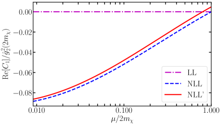
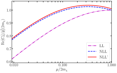
Figure 1: Evolution of the real part of the matching coefficients in various approximations for $m_{\chi}=5$ TeV, $\mu_{h}=2m_{\chi}$.

In Figure 1 we show the evolved coefficient functions in the above mentioned approximations. The evolution equation is solved by numerical solution of the differential equation in the given approximation after solving the coupled system of renormalization group equations for the three gauge couplings, the top Yukawa and the Higgs self-coupling in the two-loop approximation. The input values for the couplings are specified at the scale $m_{Z}=91.1876\,$GeV in the $\overline{\rm MS}$ scheme: $\hat{\alpha}_{2}(m_{Z})=0.0350009$, $\hat{\alpha}_{3}(m_{Z})=0.1181$, $\hat{s}_{W}^{2}(m_{Z})=\hat{g}_{1}^{2}/(\hat{g}_{1}^{2}+\hat{g}_{2}^{2})(m_{Z})=0.222958$, $\hat{\lambda}_{t}(m_{Z})=0.952957$, $\lambda(m_{Z})=0.132944$. The $\overline{\rm MS}$ gauge couplings are computed via one-loop relations from $m_{Z}$, $m_{W}=80.385\,$ GeV, the on-shell electromagnetic coupling $\alpha_{\text{OS}}(m_{Z})=1/128.943$ at the $Z$ mass scale, and the top Yukawa and Higgs self-coupling, which enter our calculation only implicitly through the two-loop evolution of the gauge couplings, via tree-level relations to $\overline{m}_{t}(\overline{m}_{t})=163.35\,$GeV (corresponding to the top pole mass 173.2 GeV at four loops) and $m_{H}=125.0\,$GeV.

2.2.2 Soft functions

The soft renormalization factor of the annihilation vertex is given by the vacuum expectation value of the Wilson lines that arise from decoupling soft EW gauge bosons from the fields that appear in the operators ${\cal O}_{i}$. In (6) the soft factor $D^{i}_{I,VW}$ is defined in the basis of DM two-particle states with respect to the SU(2) indices of the DM bilinear, which corresponds to the definition

$$D^{i}_{I,VW}=K_{I,ab}\,\langle 0|[Y_{v}^{\dagger}T_{i}^{AB}Y_{v}]_{ab}\,Y_{n_{-}}^{AV}Y_{n_{+}}^{BW}|0\rangle\,.$$ (22)

The matrix $K$ takes the linear combination appropriate to the two-particle state $I$, and $T_{1}^{AB}=\delta^{AB}$, $T_{2}^{AB}=\frac{1}{2}\,\{T^{A},T^{B}\}$ for the two operators $i=1,2$. The light-like Wilson lines $Y_{n_{-}}^{AV},Y_{n_{+}}^{BW}$ arise from the gauge fields and are in the adjoint representation. The time-like Wilson line $Y_{v}$ is in the isospin-$j$ representation of the DM field. All four Wilson lines extend from $x=0$ to infinity in their respective directions. Note that although $V,W=1,2,3$ are the gauge boson indices referring to $W^{A}$ rather than the mass eigenstates $W^{\pm}$, $Z$, $\gamma$, the soft function lives at the electroweak scale and must be computed with the Feynman rules of the SM after electroweak symmetry breaking, including gauge boson masses, contrary to the hard coefficient functions discussed above, which can be computed in the unbroken theory, neglecting the masses of the SM particles.

The requirement of an observed energetic photon implies $Y=W=3$, and then electric charge conservation implies that also $V=X=3$. Hence, only the index values $V,W,X,Y=3$ contribute to (6), so the corresponding sums disappear. The NLL’ approximation requires the one-loop calculation of every function that appears in the factorization formula. For the triplet (‘wino’) model we find

$$D^{1}_{(00),\,33}(\mu,\nu)=1+\frac{\hat{g}_{2}^{2}(\mu)}{16\pi^{2}}\Bigg{(}8\ln^{2}\frac{m_{W}}{\mu}-8i\pi\ln\frac{m_{W}}{\mu}-\frac{\pi^{2}}{3}-16\ln\frac{m_{W}}{\mu}\ln\frac{m_{W}}{\nu}\Bigg{)}\,,\qquad$$ (23)

$$D^{2}_{(00),\,33}(\mu,\nu)=\frac{\hat{g}_{2}^{2}(\mu)}{16\pi^{2}}\,(8-8i\pi)\ln\frac{m_{W}}{\mu}\,,$$ (24)

$$D^{1}_{(+-),\,33}(\mu,\nu)=D^{1}_{(00),\,33}(\mu,\nu)\,,$$ (25)

$$D^{2}_{(+-),\,33}(\mu,\nu)=D^{1}_{(00),\,33}(\mu,\nu)-\frac{1}{2}\,D^{2}_{(00),\,33}(\mu,\nu)$$ (26)

for the two operators and the two distinct two-particle states $I=00,+-$. Since there are three regions with equal virtuality ${\cal O}(m_{W}^{2})$ but different light-cone momentum component $n_{+}\cdot k$, the soft function is not well defined with only a dimensional regulator. We use the rapidity regulator [19] in addition to dimensional regularization to obtain the above result and the jet functions below. The scale $\nu$ is related to the rapidity regulator. The soft function contains no large logarithms if $\mu,\nu\sim{\cal O}(m_{W})$.

2.2.3 Photon jet function

The ‘jet’ function for the exclusive anti-collinear photon state is defined by the squared matrix element

$$-g_{\perp,\mu\nu}\,Z_{\gamma}^{BC}=\sum_{\lambda}\,\langle 0|\mathcal{A}^{B}_{\perp\bar{c},\mu}(0)|\gamma(p_{\gamma},\lambda)\rangle\langle\gamma(p_{\gamma},\lambda)|\mathcal{A}^{C}_{\perp\bar{c},\nu}(0)|0\rangle$$ (27)

of the three-component of the transverse SU(2) gauge field. $\mathcal{A}^{B}_{\perp\bar{c},\mu}$ denotes the gauge field dressed with anti-collinear Wilson lines, $\hat{g}_{2}\mathcal{A}^{B}_{\perp\bar{c},\mu}T^{B}=W^{\dagger}_{\bar{c}}[iD_{\perp\bar{c},\mu}W_{\bar{c}}]$, hence $Z^{33}_{\gamma}/\hat{s}_{W}^{2}$ can be interpreted as the on-shell photon field renormalization constant in light-cone gauge.

At the one-loop order we obtain

$$Z_{\gamma}^{33}(\mu,\nu) = \hat{s}_{W}^{2}(\mu)-\frac{\hat{\alpha}(\mu)}{4\pi}\,\bigg{\{}-16\ln\frac{m_{W}}{\mu}\ln\frac{2m_{\chi}}{\nu}+8\ln\frac{m_{W}}{\mu}$$ (28)

$$-\,\hat{s}^{2}_{W}(\mu)\frac{80}{9}\bigg{(}\ln\frac{m_{Z}^{2}}{\mu^{2}}-\frac{5}{3}\bigg{)}-\hat{s}^{2}_{W}(\mu)\frac{16}{9}\ln\frac{m_{t}^{2}}{\mu^{2}}$$

$$+\,\hat{s}^{2}_{W}(\mu)\bigg{(}3\ln\frac{m_{W}^{2}}{\mu^{2}}-\frac{2}{3}\bigg{)}-4\frac{m_{W}^{2}}{m_{Z}^{2}}\ln\frac{m_{W}^{2}}{\mu^{2}}\bigg{\}}-\hat{s}_{W}^{2}(\mu)\Delta\alpha\,,$$

where $\Delta\alpha$ determines the difference between the fine structure constant $\alpha=1/137.036$ and $\alpha_{\rm OS}(m_{Z})=\alpha/(1-\Delta\alpha)$.

2.2.4 Jet function of the unobserved final state

The jet function pertaining to the inclusive (unobserved) collinear final state is defined as the total discontinuity

$$J^{BC}(p^{2})=\frac{1}{\pi}\,\text{Im}\big{[}\,i\mathcal{J}^{BC}(p^{2})\big{]}$$ (29)

of the gauge-boson two-point function

$$-g_{\mu\nu}\,\mathcal{J}^{BC}(p^{2})\equiv\int d^{4}x\,e^{ip\cdot x}\langle 0|\mathbf{T}\big{\{}\mathcal{A}^{B}_{\perp c,\mu}(x)\,\mathcal{A}_{\perp c,\nu}^{C}(0)\big{\}}|0\rangle\,.$$ (30)

Again the field $\mathcal{A}^{B}_{\perp c,\mu}$ refers to the collinear gauge-invariant gauge field, which equals the ordinary gauge field in light-cone gauge.

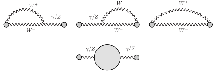
Figure 2: Wilson-line and self-energy type one-loop contributions to the jet function.

We compute the 33 component in Feynman gauge to the one-loop order and write $J^{33}(p^{2})$ in the form

$$J^{33}(p^{2})=\hat{s}_{W}^{2}(\mu)\,\delta(p^{2})+\hat{c}_{W}^{2}(\mu)\,\delta(p^{2}-m_{Z}^{2})+J^{33}_{\text{Wilson line}}(p^{2})+J^{33}_{\text{se}}(p^{2})\,.$$ (31)

The one-loop correction is split into two contributions, of which the first refers to diagrams that involve at least one contraction with a gauge field from a Wilson line in the definition of $\mathcal{A}^{B}_{\perp c,\mu}$ and the second to the remaining diagrams, which are of self-energy type, as shown in the first and second line of Fig. 2, respectively. Only the Wilson-line diagrams require the rapidity regulator, and their sum is given by

$$J^{33}_{\text{Wilson line}}(p^{2},\mu,\nu) = -\frac{\hat{s}^{2}_{W}(\mu)\hat{g}^{2}_{2}(\mu)}{16\pi^{2}}\bigg{\{}\delta(p^{2})\bigg{[}-16\ln\frac{m_{W}}{\mu}\ln\frac{2m_{\chi}}{\nu}+8\ln\frac{m_{W}}{\mu}\bigg{]}$$ (32)

$$+\,\frac{1}{p^{2}}\,\theta(p^{2}-4m^{2}_{W})\Big{[}4\beta+8\ln\frac{1-\beta}{1+\beta}\,\Big{]}\bigg{\}}$$

$$-\,\frac{\hat{c}^{2}_{W}(\mu)\hat{g}^{2}_{2}(\mu)}{16\pi^{2}}\bigg{\{}\delta(p^{2}-m^{2}_{Z})\bigg{[}-16\ln\frac{m_{W}}{\mu}\ln\frac{2m_{\chi}}{\nu}+8\ln\frac{m_{W}}{\mu}-8+4\pi^{2}$$

$$+\,4\pi\bar{\beta}_{Z}-(16\pi+8\bar{\beta}_{Z})\arctan(\bar{\beta}_{Z})+16\arctan^{2}(\bar{\beta}_{Z})\bigg{]}$$

$$+\,\frac{1}{p^{2}-m^{2}_{Z}}\,\theta(p^{2}-4m^{2}_{W})\Big{[}4\beta+8\ln\frac{1-\beta}{1+\beta}\,\Big{]}\bigg{\}}\,,$$

where

$$\beta=\sqrt{1-\frac{4m^{2}_{W}}{p^{2}}}\,,\qquad\bar{\beta}_{Z}=\sqrt{\,\frac{4m^{2}_{W}}{m^{2}_{Z}}-1}\,.$$ (33)

The self-energy type contribution $J^{33}_{\text{se}}(p^{2})$ can be expressed in terms of conventional one-loop gauge-boson self-energies, which can be found, for example in [20]. We have taken the massless-quark limit of these expressions except for the top quark. We will provide the lengthy expressions in the detailed write-up.

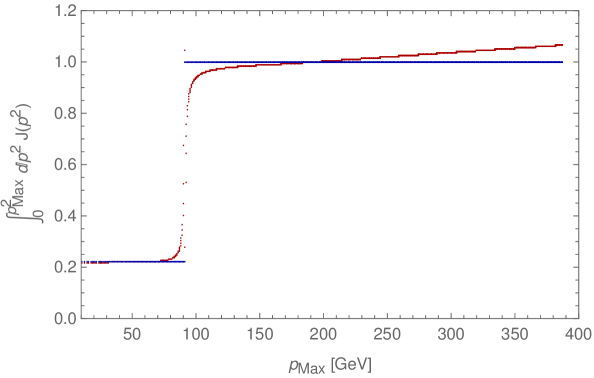
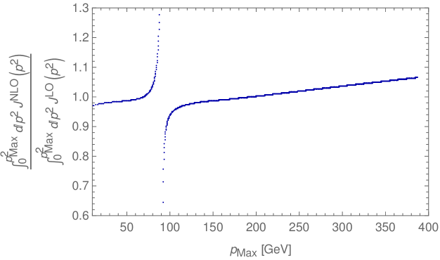
Figure 3: Integrated jet function (upper panel) at next-to-leading order for $\mu=\nu=m_{W}$ and $m_{\chi}=2\,$TeV. The straight lines represent the leading-order result. The lower panel shows the integrated jet function at NLO normalized to its LO value.

In Fig. 3 we show the dependence of the integrated jet function on the invariant mass of the unobserved collinear final state. The integrated function jumps from a value around $\hat{s}_{W}^{2}(m_{W})$ to a value around 1 as the invariant mass passes through $m_{Z}$, and then slowly increases. The range shown contains the $W^{+}W^{-}$, $ZH$ and $t\bar{t}$ thresholds ($m_{t}=173.2$ GeV is used here), which, however, are barely visible. The singularity of the NLO correction near $m_{Z}$ can be removed by a proper treatment of $Z$ boson resonance. However, below we will adopt values $E^{\gamma}_{\rm res}>m_{Z}^{2}/(4m_{\chi})$, which implies that $p^{2}_{\rm max}$ is always larger than $m_{Z}^{2}$.

The jet functions contain no large logarithms when $\mu={\cal O}(m_{W})$ and $\nu={\cal O}(m_{\chi})$. The ‘rapidity logarithms’ related to the different value of $\nu$ that minimizes the logarithms in the soft and jet functions, respectively, can be summed at NLL’ by solving the rapidity renormalization group equations [19] in the one-loop approximation. For the case at hand we find

$$V(\mu_{W},\nu_{s},\nu_{j})=\exp\left[\frac{4c_{2}(\text{ad})}{\beta_{0,\rm SU(2)}}\ln\left(\frac{\hat{\alpha}_{2}(\mu_{W})}{\hat{\alpha}_{2}(m_{W})}\right)\ln\frac{\nu_{j}^{2}}{\nu_{s}^{2}}\,\right].$$ (34)

We checked that in the sum of all contributions the poles in the dimensional and rapidity regulator cancel. The hard, soft and jet functions above are defined by minimally subtracting the poles.

2.2.5 Ultrasoft function

The kinematics of the process does not allow soft radiation with momentum of order $m_{W}$ into the final state, which prohibits EW gauge boson radiation. However, radiation of photons and light quarks with masses of order or less than $m_{W}^{2}/m_{\chi}$ is possible, which implies the convolution of the unobserved-final state jet function with an ultrasoft function accounting for the energy taken away from the collinear final state by ultrasoft radiation. The ultrasoft function is defined in terms of Wilson lines of ultrasoft photons and depends on the electric charges and directions of the particles in the initial and final state. After factoring the Sommerfeld effect, also the $\chi^{+}\chi^{-}$ initial state must be considered. But for the S-wave annihilation operators ${\cal O}_{i}$ only the total charge of the initial state is relevant for ultrasoft radiation, which vanishes. Furthermore, only the electrically neutral 33 components of the (anti) collinear functions appear for the $\gamma+X$ final state. We therefore conclude that the ultrasoft function is trivial, $S_{\gamma}(\omega)=\delta(\omega)\,.$ For this reason did not indicate the ultrasoft scale dependence of the functions in (6), and the convolution integral in (6) disappears.

2.2.6 Sommerfeld factor

The various functions discussed above are assembled according to (6) into the annihilation matrix $\Gamma_{IJ}$ of the $\chi^{0}\chi^{0}$ and $\chi^{+}\chi^{-}$ DM two-particle states. In the process we checked the consistency of (6) by verifying that after renormalizing the parameters in the tree-level annhilation rates, all $1/\epsilon$ and rapidity regulator poles that appear in the various factors of the factorization formula cancel among each other, leaving logarithms consistent with the anomalous dimensions of these factors. The photon energy spectrum is then obtained according to (5) by tracing this matrix with the Sommerfeld factor $S_{IJ}$. For the fermionic DM triplet model, the Sommerfeld factors were first computed in [3]. In the present work we employ the modified variable phase method [13] for solving the Schrödinger equation and, different from the above, use the on-shell value $\alpha_{2}=0.0347935$ of the SU(2) coupling as well as $\alpha_{\rm OS}(m_{Z})$ in the Yukawa-Coulomb potential for the two-state system. Near the Sommerfeld resonance, the result is very sensitive to the mass splitting between the electrically charged and neutral members of the triplet. The mass splitting with two-loop accuracy can be inferred from [21, 22], and is given after adjustment to our input coupling parameters by

$$\delta m_{\chi}=164.1\,\text{MeV}.$$ (35)

The first and second Sommerfeld resonances are located at 2.285 TeV and 8.817 TeV, respectively, for the coupling parameters and mass splitting employed in this work.

3 Results

It is straightforward to calculate the one-dimensional integral (3) that defines the $\gamma+X$ yield from DM pair annihilation in a photon energy bin of size $E^{\gamma}_{\rm res}$. For the discussion below we shall assume $4m_{\chi}E^{\gamma}_{\rm res}=(300\,\text{GeV})^{2}$, which implies that the unobserved final state includes $\gamma$, $Z$, $W^{+}W^{-}$, $ZH$ and light fermion pairs in the collinear jet function.

Figure 4 shows (upper panel) our results for $\langle\sigma v\rangle(E^{\gamma}_{\rm res})$ as defined in (3). The displayed DM mass range includes the first two Sommerfeld resonances. The four lines refer to the Sommerfeld-only calculation, which employs the tree-level approximation to $\Gamma_{IJ}$ (black-dotted) and the successive LL (magenta-dashed), NLL (blue-dashed) and NLL’ (red-solid) resummed expressions for the same quantities with the latter representing the best approximation.

The importance of resummation of electroweak Sudakov logarithms becomes more apparent by normalizing to the Sommerfeld-only result (lower panel). As expected and already seen in previous LL and NLL calculations [5, 6, 7, 8, 9] of related exclusive and semi-inclusive final states, resummation reduces the annihilation rate and increasingly so at larger DM mass. In the interesting mass range around 3 TeV where wino DM accounts for the observed relic density, the rate is suppressed by about a factor of two.

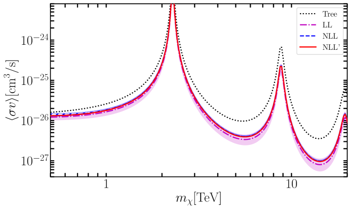
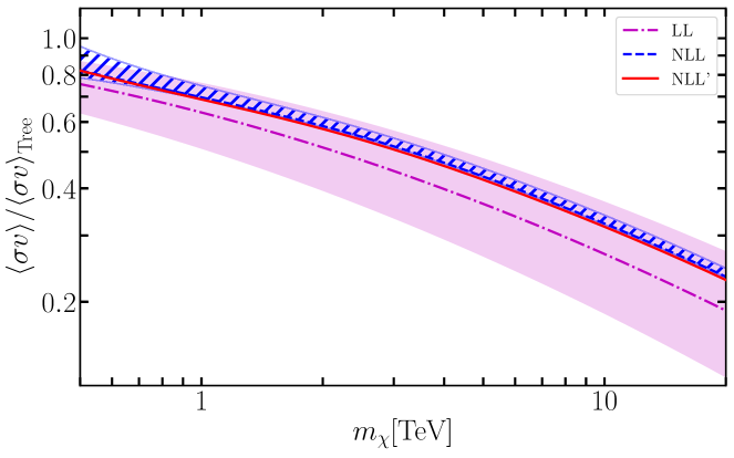
Figure 4: Integrated photon energy spectrum within $E^{\gamma}_{\text{res}}$ from the endpoint $m_{\chi}$ in the tree (Sommerfeld only) and LL, NLL, NLL’ resummed approximation. The shaded/hatched bands show the scale variation of the respective approximation as described in the text. For the NLL’ result the theoretical uncertainty is given by the thickness of the red line.

The resummed predictions are shown with theoretical uncertainty bands computed from the separate variations of the scales $\mu_{h}$, $\nu_{j}$ in the interval $[m_{\chi},4m_{\chi}]$ and the scales $\mu_{W}$, $\nu_{s}$ in $[m_{W}/2,2m_{W}]$, added in quadrature. We find that at the NLL’ order the residual theoretical uncertainty from scale dependence is negligible – in the figure it is given by the width of the red line. Our result can be compared most directly with the recent work by Baumgart et al. [11] who considered the same $\gamma+X$ final state at larger resolution $E_{\rm res}^{\gamma}\gg m_{W}$ with LL accuracy. We observe that the inclusion of one-loop corrections to the hard, soft and jet functions in our NLL’ computation has the main effect of eliminating the theoretical uncertainty of resummation by reducing the scale dependence from 24% (LL) to 3% (NLL) to 0.3% at NLL’ at $m_{\chi}=2~{}$TeV. A similar reduction of scale dependence was already observed in the NLL’ calculation of the exclusive $\gamma\gamma$, $\gamma Z$ final state [9]. In numbers we find that at $m_{\chi}=2\,$TeV (10 TeV), the ratio of the resummed to the Sommerfeld-only rate is $0.513^{+0.128}_{-0.120}$ ($0.268^{+0.101}_{-0.082}$) at LL, $0.585^{+0.032}_{-0.004}$ ($0.323^{+0.017}_{-0.002}$) at NLL and $0.575^{+0.003}_{-0.000}$ ($0.316^{+0.002}_{-0.000}$) at NLL’. The central values are evaluated at the central scales of the intervals above. We also varied all four scales simultaneously within these intervals and determined the maximal variation. The scale dependence at NLL’ with this more conservative procedure increases by about a factor of two, which does not change the general picture.

In conclusion, we computed the $\gamma+X$ spectrum near maximal photon energy from electroweak triplet (‘wino’) DM annihilation including the resummation of the Sommerfeld effect and electroweak Sudakov logarithms in the NLL’ order. The inclusion of the electroweak one-loop corrections at NLL’ renders the theoretical uncertainty of resummation negligible. It is plausible that the dominant theoretical uncertainty now arises from the fact that the non-relativistic EFT is only employed at leading order in the computation of the Sommerfeld enhancement, and from $\mathcal{O}(m_{W}/m_{\chi})$ power corrections. In a subsequent paper we shall present an extension of this work to the case of wider photon resolution, further details on the EFT framework, the derivation of the factorization formula, and a comparison with expected experimental limits. The computations performed here are presently restricted to simple DM models, which add to the SM a single electroweak multiplet. It would be of interest to extend them to more complex models such as the MSSM, which would put the analysis of indirect detection constraints for mixed DM models [23] on the same theoretical footing as for minimal models.

Acknowledgement

We thank D. Pagani and K. Urban for discussions. This work has been supported in part by the Collaborative Research Center ‘Neutrinos and Dark Matter in Astro- and Particle Physics’ (SFB 1258) and the Excellence Cluster ‘Universe’ of the Deutsche Forschungsgemeinschaft. MB thanks the Albert Einstein Institute at Bern University and the Department of Energy’s Institute for Nuclear Theory at the University of Washington for hospitality during the preparation of this work.

References

- [1] H.E.S.S. Collaboration, H. Abdallah et. al., Search for -Ray Line Signals from Dark Matter Annihilations in the Inner Galactic Halo from 10 Years of Observations with H.E.S.S., Phys. Rev. Lett. 120 (2018), no. 20 201101 [1805.05741].
- [2] CTA Consortium Collaboration, M. Actis et. al., Design concepts for the Cherenkov Telescope Array CTA: An advanced facility for ground-based high-energy gamma-ray astronomy, Exper. Astron. 32 (2011) 193–316 [1008.3703].
- [3] J. Hisano, S. Matsumoto, M. M. Nojiri and O. Saito, Non-perturbative effect on dark matter annihilation and gamma ray signature from galactic center, Phys. Rev. D71 (2005) 063528 [hep-ph/0412403].
- [4] A. Hryczuk and R. Iengo, The one-loop and Sommerfeld electroweak corrections to the Wino dark matter annihilation, JHEP 01 (2012) 163 [1111.2916]. [Erratum: JHEP06,137(2012)].
- [5] M. Baumgart, I. Z. Rothstein and V. Vaidya, Calculating the Annihilation Rate of Weakly Interacting Massive Particles, Phys. Rev. Lett. 114 (2015) 211301 [1409.4415].
- [6] M. Bauer, T. Cohen, R. J. Hill and M. P. Solon, Soft Collinear Effective Theory for Heavy WIMP Annihilation, JHEP 01 (2015) 099 [1409.7392].
- [7] M. Baumgart and V. Vaidya, Semi-inclusive wino and higgsino annihilation to LL , JHEP 03 (2016) 213 [1510.02470].
- [8] G. Ovanesyan, T. R. Slatyer and I. W. Stewart, Heavy Dark Matter Annihilation from Effective Field Theory, Phys. Rev. Lett. 114 (2015), no. 21 211302 [1409.8294].
- [9] G. Ovanesyan, N. L. Rodd, T. R. Slatyer and I. W. Stewart, One-loop correction to heavy dark matter annihilation, Phys. Rev. D95 (2017), no. 5 055001 [1612.04814].
- [10] M. Beneke, P. Falgari and C. Schwinn, Threshold resummation for pair production of coloured heavy (s)particles at hadron colliders, Nucl. Phys. B842 (2011) 414–474 [1007.5414].
- [11] M. Baumgart, T. Cohen, I. Moult, N. L. Rodd, T. R. Slatyer, M. P. Solon, I. W. Stewart and V. Vaidya, Resummed Photon Spectra for WIMP Annihilation, JHEP 03 (2018) 117 [1712.07656].
- [12] M. Cirelli, N. Fornengo and A. Strumia, Minimal dark matter, Nucl. Phys. B753 (2006) 178–194 [hep-ph/0512090].
- [13] M. Beneke, C. Hellmann and P. Ruiz-Femenia, Non-relativistic pair annihilation of nearly mass degenerate neutralinos and charginos III. Computation of the Sommerfeld enhancements, JHEP 05 (2015) 115 [1411.6924].
- [14] C. W. Bauer, D. Pirjol and I. W. Stewart, Soft collinear factorization in effective field theory, Phys. Rev. D65 (2002) 054022 [hep-ph/0109045].
- [15] M. Beneke, R. Szafron and K. Urban , work in preparation.
- [16] K. Urban, Bound-state contributions to dark matter freeze-out and annihilation, Master Thesis, Technische Universität München (2017).
- [17] M. Beneke, P. Falgari and C. Schwinn, Soft radiation in heavy-particle pair production: All-order colour structure and two-loop anomalous dimension, Nucl. Phys. B828 (2010) 69–101 [0907.1443].
- [18] A. Broggio, C. Gnendiger, A. Signer, D. Stöckinger and A. Visconti, SCET approach to regularization-scheme dependence of QCD amplitudes, JHEP 01 (2016) 078 [1506.05301].
- [19] J.-Y. Chiu, A. Jain, D. Neill and I. Z. Rothstein, A Formalism for the Systematic Treatment of Rapidity Logarithms in Quantum Field Theory, JHEP 05 (2012) 084 [1202.0814].
- [20] A. Denner, Techniques for calculation of electroweak radiative corrections at the one loop level and results for W physics at LEP-200, Fortsch. Phys. 41 (1993) 307–420 [0709.1075].
- [21] Y. Yamada, Electroweak two-loop contribution to the mass splitting within a new heavy SU(2)(L) fermion multiplet, Phys. Lett. B682 (2010) 435–440 [0906.5207].
- [22] M. Ibe, S. Matsumoto and R. Sato, Mass Splitting between Charged and Neutral Winos at Two-Loop Level, Phys. Lett. B721 (2013) 252–260 [1212.5989].
- [23] M. Beneke, A. Bharucha, A. Hryczuk, S. Recksiegel and P. Ruiz-Femenia, The last refuge of mixed wino-Higgsino dark matter, JHEP 01 (2017) 002 [1611.00804].