The Blessings of Multiple Causes

Abstract

Causal inference from observational data often assumes “ignorability,” that all confounders are observed. This assumption is standard yet untestable. However, many scientific studies involve multiple causes, different variables whose effects are simultaneously of interest. We propose the deconfounder, an algorithm that combines unsupervised machine learning and predictive model checking to perform causal inference in multiple-cause settings. The deconfounder infers a latent variable as a substitute for unobserved confounders and then uses that substitute to perform causal inference. We develop theory for the deconfounder, and show that it requires weaker assumptions than classical causal inference. We analyze its performance in three types of studies: semi-simulated data around smoking and lung cancer, semi-simulated data around genome-wide association studies, and a real dataset about actors and movie revenue. The deconfounder provides a checkable approach to estimating closer-to-truth causal effects.

Keywords: Causal inference, strong ignorability, probabilistic models

1 Introduction

Here is a frivolous, but perhaps lucrative, causal inference problem. Table 1 contains data about movies. For each movie, the table shows its cast of actors and how much money the movie made. Consider a movie producer interested in the causal effect of each actor; for example, how much does revenue increase (or decrease) if Oprah Winfrey is in the movie?

The producer wants to solve this problem with the potential outcomes approach to causality (Imbens:2015; rubin1974estimating; rubin2005causal). Following the methodology, she associates each movie to a potential outcome function, $y_{i}(\mathbf{\boldsymbol{a}})$. This function maps each possible cast $\mathbf{\boldsymbol{a}}$ to its revenue if the movie $i$ had that cast. (The cast $\mathbf{\boldsymbol{a}}$ is a binary vector with one element per actor; each element encodes whether the actor is in the movie.) The potential outcome function encodes, for example, how much money Star Wars would have made if Robert Redford replaced Harrison Ford as Han Solo. When doing causal inference, the producer’s goal is to estimate something about the population distribution of $Y_{i}(\mathbf{\boldsymbol{a}})$. For example, she might consider a particular cast $\mathbf{\boldsymbol{a}}$ and estimate the expected revenue of a movie with that cast, $\mathbb{E}\left[Y_{i}(\mathbf{\boldsymbol{a}})\right]$.

Classical causal inference from observational data (like Table 1) is a difficult enterprise and requires strong assumptions. The challenge is that the dataset is limited; it contains the revenue of each movie, but only at its assigned cast. However, what this paper is about is that the producer’s problem is not a classical causal inference. While causal inference usually considers a single possible cause, such as whether a subject receives a drug or a control, our producer is considering a multiple causal inference, where each actor is a possible cause. This paper shows how multiple causal inference can be easier than classical causal inference. Thanks to the multiplicity of causes, the producer can make valid causal inferences under weaker assumptions than the classical approach requires.

Let’s discuss the producer’s inference in more detail: how can she calculate $\mathbb{E}\left[Y_{i}(\mathbf{\boldsymbol{a}})\right]$? Naively, she subsets the data in Table 1 to those with cast equal to $\mathbf{\boldsymbol{a}}$, and then computes a Monte Carlo estimate of the revenue. This procedure is unbiased when $\mathbb{E}\left[Y_{i}(\mathbf{\boldsymbol{a}})\right]=\mathbb{E}\left[Y_{i}(\mathbf{\boldsymbol{a}})\,|\,\mathbf{\boldsymbol{A}}_{i}=\mathbf{\boldsymbol{a}}\right]$.

But there is a problem. The data in Table 1 hide confounders, variables that affect both the causes and the effect. For example, every movie has a genre, such as comedy, action, or romance. This genre has an effect on both who is in the cast and the revenue. (E.g., action movies cast a certain set of actors and tend to make more money than comedies.) When left unobserved, the genre of the movie produces a statistical dependence between whether an actor is in it and its revenue; this dependence biases the causal estimates, $\mathbb{E}\left[Y_{i}(\mathbf{\boldsymbol{a}})\,|\,\mathbf{\boldsymbol{A}}_{i}=\mathbf{\boldsymbol{a}}\right]\neq\mathbb{E}\left[Y_{i}(\mathbf{\boldsymbol{a}})\right]$.

Thus the main activities of classical causal inference are to identify, measure, and control for confounders. Suppose the producer measures confounders for each movie $w_{i}$. Then inference is simple: use the data (now with confounders) to take Monte Carlo estimates of $\mathbb{E}\left[\mathbb{E}\left[Y_{i}(\mathbf{\boldsymbol{a}})\,|\,W_{i},\mathbf{\boldsymbol{A}}_{i}=\mathbf{\boldsymbol{a}}\right]\right]$; this iterated expectation “controls” for the confounders. But the problem is that whether the estimate is equal to $\mathbb{E}\left[Y_{i}(\mathbf{\boldsymbol{a}})\right]$ rests on a big and uncheckable assumption: there are no other confounders. For many applied causal inference problems, this assumption is a leap of faith.

Title	Cast	Revenue
Avatar	{Sam Worthington, Zoe Saldana, Sigourney Weaver, Stephen Lang, $\ldots$ }	$2788M
Titanic	{Kate Winslet, Leonardo DiCaprio, Frances Fisher, Billy Zane, $\ldots$ }	$1845M
The Avengers	{Robert Downey Jr., Chris Evans, Mark Ruffalo, Chris Hemsworth, $\ldots$ }	$1520M
Jurassic World	{Chris Pratt, Bryce Dallas Howard, Irrfan Khan, Vincent D’Onofrio, $\ldots$ }	$1514M
Furious 7	{Vin Diesel, Paul Walker, Dwayne Johnson, Michelle Rodriguez, $\ldots$ }	$1506M
$\quad\quad\vdots$	$\quad\vdots\quad$	$\quad\vdots\quad$

Table 1: Top earning movies in the TMDB dataset

We develop the deconfounder, an alternative method for the producer who worries about missing a confounder. First the producer finds and fits a good latent-variable model to capture the dependence among actors. It should be a factor model, one that contains a per-movie latent variable that renders the assigned cast conditionally independent. (Probabilistic principal component analysis (tipping1999probabilistic) is a simple example, but there are many others.) Given the model, she then estimates the per-movie variable for each cast in the dataset; this estimated variable is a substitute for unobserved confounders. Finally, she controls for the substitute confounder and obtains valid causal inferences.

The deconfounder capitalizes on the dependency structure of the observed casts, using patterns of how actors tend to appear together in movies as indirect evidence for confounders in the data. Thus the producer replaces an uncheckable search for possible confounders with the checkable goal of building a good factor model of observed casts.

All methods for causal inference using observational data are based on assumptions. Here we make two. First, we assume that the fitted latent-variable model is a good model of the assigned causes. Happily, this assumption is testable; we will use predictive checks to assess how well the fitted model captures the data. Second, we assume that there are no unobserved single-cause confounders, variables that affect one cause (e.g., actor) and the potential outcome function (e.g., revenue). While this assumption is not testable, it is weaker than the usual assumption of ignorability, i.e., no unobserved confounders.

Beyond making movies, many causal inference problems, especially from observational data, also classify as multiple causal inference. Such problems arise in many fields.

• Genome-wide association studies (GWAS). In GWAS, biologists want to know how genes causally connect to traits (stephens2009bayesian; visscher201710). The assigned causes are alleles on the genome, often encoded as either being common (“major”) or uncommon (“minor”), and the effect is the trait under study. Confounders, such as shared ancestry among the population, bias naive estimates of the effect of genes. We study GWAS problems in Section 3.2.

• Computational neuroscience. Neuroscientists want to know how specific neurons or brain measurements affect behavior and thoughts (churchland2012neural). The possible causes are multiple measurements about the brain’s activity, e.g., one per neuron, and the effect is a measured behavior. Confounders, particularly through dependencies among neural activity, bias the estimated connections between brain activity and behavior.

• Social science. Sociologists and policy-makers want to know how social programs affect social outcomes, such as poverty levels and upward mobility (Morgan:2015). However, individuals may enroll in several such programs, blurring information about their possible effects. In social science, controlled experiments are difficult to engineer; using observational data for causal inference is typically the only option.

• Medicine. Doctors want to know how medical treatments affect the progression of disease. The multiple causes are medications and procedures; the outcome is a measurement of a disease (e.g., a lab test). There are many confounders—such as when and where a patient is treated or the treatment preferences of the attending doctor—and these variables bias the estimates of effects. While gold-standard data from clinical trials are expensive to obtain, the abundance of electronic health records could inform medical practices.

Causal inference in each of these fields can use the deconfounder. Fit a good factor model of the assigned causes, infer substitute confounders, and use the substitutes in causal inference.

Related work.  The deconfounder relates to several threads of research in causal inference.

Probabilistic modeling for causal inference. stegle2010probabilistic use Gaussian processes to depict causal mechanisms; zhang2009identifiability study post-nonlinear causal models and their identifiability; mckeigue2010sparse builds on sparse methods to infer causal structures; moghaddass2016factorized generalize the self-controlled case series method to multiple causes and multiple outcomes using factor models. More recently, louizos2017causal use variational autoencoders to infer unobserved confounders, shah2018rsvp develop projection-based techniques for high-dimensional covariance estimation under latent confounding, and kaltenpoth2019we leverages information theory principles to differentiate causal and confounded connections.

With a related goal, tran2017implicit build implicit causal models. Like the GWAS example in this paper (Section 3.2), they take an explicit causal view of genome-wide association studies (gwas), treating the single-nucleotide polymorphisms (snps) as the multiple causes. They connect implicit probabilistic models and nonparametric structural equation models for causal inference (Pearl:2009a), and develop inference algorithms for capturing shared confounding. heckerman2018accounting studies the same scenario with multiple linear regression, where observing many causes makes it possible to account for shared confounders. Multiple causal inference and latent confounding was also formalized by ranganath2018multiple, who take an information-theoretic approach.

Our work complements all of these works. These works rest on Pearl’s causal framework (Pearl:2009a); they hypothesize a causal graph with confounders, causes, and outcomes. We develop the deconfounder in the context of the potential outcomes framework (Imbens:2015; rubin1974estimating; rubin2005causal).

Analyzing gwas. In gwas, latent population structure is an important unobserved confounder. pritchard2000association propose a probabilistic admixture model for unsupervised ancestry inference. price2006principal and astle2009population estimate the unobserved population structure using the principal components of the genotype matrix. yu2006unified and kang2010variance estimate the population structure via the “kinship matrix” on the genotypes. song2015testing and hao2015probabilistic rely on factor analysis and admixture models to estimate the population structure. GTEx2017 adopt a similar idea to study the effect of genetic variations on gene expression levels. These methods can be seen as variants of the deconfounder (see Section 2.5). The deconfounder gives them a rigorous causal justification, provides principled ways to compare them, and suggests an array of new approaches. We study gwas data in Section 3.2.

Assessing the ignorability assumption. rosenbaum1983central demonstrates that ignorability and a good propensity score model are sufficient to perform causal inference with observational data. Many subsequent efforts assess the plausibility of ignorability. For example, robins2000sensitivity; gilbert2003sensitivity; imai2004causal develop sensitivity analysis in various contexts, though focusing on data with a single cause. In contrast, this work uses predictive model checks to assess unconfoundedness with multiple causes. More recently, sharma2016split leveraged auxillary outcome data to test for confounding in time series data; janzing2018detecting; janzing2018detecting2; liu2018confounder developed tests for non-confounding in multivariate linear regression. Here we work without auxiliary data, focus on causal estimation, as opposed to testing, and move beyond linear models.

The (generalized) propensity score. schneeweiss2009high; mccaffrey2004propensity; lee2010improving and many others develop and evaluate different models for assigned causes. In particular, chernozhukov2017double introduce a semiparametric assignment model; they propose a principled way of correcting for the bias that arises when regularizing or overfitting the assignment model. This work introduces latent variables into the model. The multiplicity of causes enables us to infer these latent variables and then use them as substitutes for unobserved confounders.

Classical causal inference with multiple treatments. lopez2017estimation; mccaffrey2013tutorial; zanutto2005using; rassen2011simultaneously; lechner2001identification; feng2012generalized extend classical matching, subclassification, and weighting to multiple treatments, always assuming ignorability. This work relaxes that assumption.

This paper.  Section 2 reviews classical causal inference, sets up multiple causal inference, presents the deconfounder, and describes its identification strategy and assumptions. Section 3 presents three empirical studies, two semi-synthetic and one real. Section 4 further develops theory around the deconfounder and establishes causal identification. Finally, Section 5 concludes the paper with a discussion.

2 Multiple causal inference with the deconfounder

2.1 A classical approach to multiple causal inference

We first describe multiple causal inference. There are $m$ possible causes, encoded in a vector $\mathbf{\boldsymbol{a}}=(a_{1},\ldots,a_{m})$. We can consider a variety of types: real-valued causes, binary causes, integer causes, and so on. In the actor example, the causes are binary: $a_{j}$ encodes whether actor $j$ is in the movie.

For each individual $i$ (movie) there is a potential outcome function that maps configurations of causes to the outcome (revenue). We focus on real-valued outcomes. For the $i$th movie, the potential outcome function maps each possible cast to the log of its revenue, $y_{i}(\mathbf{\boldsymbol{a}}):\{0,1\}^{m}\rightarrow\mathbb{R}$. Note $y_{i}(\mathbf{\boldsymbol{a}})$ is a function. It maps every possible cast of actors to the movie’s revenue for that cast.

The goal of causal inference is to characterize the sampling distribution of the potential outcomes $Y_{i}(\mathbf{\boldsymbol{a}})$ for each configuration of the causes $\mathbf{\boldsymbol{a}}$. This distribution provides causal inferences, such as the expected outcome for a particular array of causes (a particular cast of actors) $\mu(\mathbf{\boldsymbol{a}})=\mathbb{E}\left[Y_{i}(\mathbf{\boldsymbol{a}})\right]$ or the average effect of individual causes (how much a particular actor contributes to revenue).

To help make causal inferences, we draw data from the sampling distribution of assigned causes $\mathbf{\boldsymbol{a}}_{i}$ (the cast of movie $i$) and realized outcomes $y_{i}(\mathbf{\boldsymbol{a}}_{i})$ (its revenue). The data is $\mathcal{D}=\{(\mathbf{\boldsymbol{a}}_{i},y_{i}(\mathbf{\boldsymbol{a}}_{i})\}\,\,\,i=1,\ldots,n$. Note we only observe the outcome for the assigned causes $y_{i}(\mathbf{\boldsymbol{a}}_{i})$, which is just one of the values of the potential outcome function. But we want to use such data to characterize the full distribution of $Y_{i}(\mathbf{\boldsymbol{a}})$ for any $\mathbf{\boldsymbol{a}}$; this is the “fundamental problem of causal inference” (Holland:1986).

To estimate $\mu(\mathbf{\boldsymbol{a}})$, consider using the data to calculate conditional Monte Carlo approximations of $\mathbb{E}\left[Y_{i}(\mathbf{\boldsymbol{a}})\,|\,\mathbf{\boldsymbol{A}}_{i}=\mathbf{\boldsymbol{a}}\right]$. These estimates are simply averages of the outcomes for each configuration of the causes. But this approach may not be accurate. There might be unobserved confounders—hidden variables that affect both the assigned causes $\mathbf{\boldsymbol{A}}_{i}$ and the potential outcome function $Y_{i}(\mathbf{\boldsymbol{a}})$. When there are unobserved confounders, the assigned causes are correlated with the observed outcome. Consequently, Monte Carlo estimates of $\mu(\mathbf{\boldsymbol{a}})$ are biased,

$$\mathbb{E}\left[Y_{i}(\mathbf{\boldsymbol{a}})\,|\,\mathbf{\boldsymbol{A}}_{i}=\mathbf{\boldsymbol{a}}\right]\neq\mathbb{E}\left[Y_{i}(\mathbf{\boldsymbol{a}})\right].$$ (1)

We can estimate $\mathbb{E}\left[Y_{i}(\mathbf{\boldsymbol{a}})\,|\,\mathbf{\boldsymbol{A}}_{i}=\mathbf{\boldsymbol{a}}\right]$ with the dataset; but the goal is to estimate $\mathbb{E}\left[Y_{i}(\mathbf{\boldsymbol{a}})\right]$.

Suppose we measure covariates $x_{i}$ and append to each data point, $\mathcal{D}=\{(\mathbf{\boldsymbol{a}}_{i},x_{i},y_{i}(\mathbf{\boldsymbol{a}}_{i})\}\,\,\,i=1,\ldots,n$. If these covariates contain all confounders then

$$\mathbb{E}\left[\mathbb{E}\left[Y_{i}(\mathbf{\boldsymbol{a}})\,|\,X_{i},\mathbf{\boldsymbol{A}}_{i}=\mathbf{\boldsymbol{a}}\right]\right]=\mathbb{E}\left[Y_{i}(\mathbf{\boldsymbol{a}})\right].$$ (2)

Using the augmented dataset, we can estimate the left side with Monte Carlo; thus we can estimate $\mathbb{E}\left[Y_{i}(\mathbf{\boldsymbol{a}})\right]$.

Equation 2 is true when $X$ capture all confounders. More precisely, it is true under the assumption of (weak) ignorability (rosenbaum1983central; imai2004causal): conditional on observed $X$, the assigned causes are independent of the potential outcomes,

$$\mathbf{\boldsymbol{A}}_{i}\mathchoice{\mathrel{\hbox to0.0pt{$\displaystyle\perp$\hss}\mkern 2.0mu{\displaystyle\perp}}}{\mathrel{\hbox to0.0pt{$\textstyle\perp$\hss}\mkern 2.0mu{\textstyle\perp}}}{\mathrel{\hbox to0.0pt{$\scriptstyle\perp$\hss}\mkern 2.0mu{\scriptstyle\perp}}}{\mathrel{\hbox to0.0pt{$\scriptscriptstyle\perp$\hss}\mkern 2.0mu{\scriptscriptstyle\perp}}}Y_{i}(\mathbf{\boldsymbol{a}})\,|\,X_{i}\qquad\forall\mathbf{\boldsymbol{a}}.$$ (3)

The nuance is that Equation 3 needs to hold for all possible $\mathbf{\boldsymbol{a}}$’s, not only for the value of $Y_{i}(\mathbf{\boldsymbol{a}})$ at the assigned causes. Ignorability implies no unobserved confounders.

Equation 2 underlies the practice of causal inference: find and measure the confounders, estimate conditional expectations, and average. In the introduction, for example, we pointed out that the genre of the movie is a confounder to causal inference of movie revenues. The genre affects both which cast is selected and the potential earnings of the film. But the assumption that there are no unobserved confounders is significant. One of the central challenges around causal inference from observational data is that ignorability is untestable—it fundamentally depends on the entire potential outcome function, of which we only observe one value (Holland:1986).

2.2 The deconfounder: Multiple causal inference without ignorability

We now develop the deconfounder, an algorithm that exploits the multiplicity of causes to sidestep the search for confounders. There are three steps. First, find a good latent variable model of the assignment mechanism $p(z,a_{1},\ldots,a_{m})$, where $z$ is a local factor. Second, use the model to infer the latent variable for each individual $p(z_{i}\,|\,a_{i1},\ldots,a_{im})$. Finally, use the inferred variable as a substitute for unobserved confounders and form causal inferences. The deconfounder replaces an uncheckable search for possible confounders with the checkable goal of building a good model of assigned causes.

We first explain the method in more detail. Then we explain why and when it provides unbiased causal inferences.

In the first step of the deconfounder, define and fit a probabilistic factor model to capture the joint distribution of causes $p(a_{1},\ldots,a_{m})$. A factor model posits per-individual latent variables $Z_{i}$, which we call local factors, and uses them to model the assigned causes. The model is

$$\begin{split}Z_{i}&\sim p(\cdot\,|\,\alpha)\quad i=1,\ldots,n,\\ A_{ij}\,|\,Z_{i}&\sim p(\cdot\,|\,z_{i},\theta_{j})\quad j=1,\ldots,m,\end{split}$$ (4)

where $\alpha$ parameterizes the distribution of $Z_{i}$ and $\theta_{j}$ parameterizes the per-cause distribution of $A_{ij}$. Notice that $Z_{i}$ can be multi-dimensional. Factor models encompass many methods from Bayesian statistics and probabilistic machine learning. Examples include matrix factorization (tipping1999probabilistic), mixture models (mclachlan1988mixture), mixed-membership models (pritchard2000association; blei2003latent; airoldi2008mixed; erosheva2003bayesian), and deep generative models (neal1990learning; ranganath2015deep; ranganath2016hierarchical; tran2017deep; rezende2015variational; mohamed2016learning; kingma2013auto). One can fit using any appropriate method, such as maximum likelihood estimation or Bayesian inference. And exact fitting is not required; one can use approximate methods like the EM algorithm, Markov chain Monte Carlo, and variational inference. What the deconfounder requires is that the fitted factor model provides an accurate approximation of the population distribution of $p(\mathbf{\boldsymbol{A}})$.

In the next step, use the fitted factor model to calculate the conditional expectation of each individual’s local factor weights $\hat{z}_{i}=\mathbb{E}_{M}\left[Z_{i}\,|\,\mathbf{\boldsymbol{A}}_{i}=\mathbf{\boldsymbol{a}}_{i}\right]$. We emphasize that this expectation is from the fitted model $M$ (not the population distribution). Again, one can use approximate expectations.

In the final step, condition on $\hat{z}_{i}$ as a substitute confounder and proceed with causal inference. For example, we can estimate $\mathbb{E}\left[\mathbb{E}\left[Y_{i}(\mathbf{\boldsymbol{a}})\,|\,\hat{Z}_{i},\mathbf{\boldsymbol{A}}_{i}=\mathbf{\boldsymbol{a}}\right]\right]$. The main idea is this: if the factor model captures the distribution of assigned causes—a testable proposition—then we can safely use $\hat{z}_{i}$ as a variable that contains the confounders.

Why is this strategy sensible? Assume the fitted factor model captures the (unconditional) distribution of assigned causes $p(a_{i1},\ldots,a_{im})$. This means that all causes are conditionally independent given the local latent factors,

$$p(a_{i1},\ldots,a_{im}\,|\,z_{i})=\prod_{j=1}^{m}p(a_{ij}\,|\,z_{i}).$$ (5)

Now make an additional assumption: there are no single-cause confounders, a variable that affects just one of the assigned causes and on the potential outcome function. (More precisely, we need to have observed all the single-cause confounders.) With this assumption, the independence statement of Equation 5 implies ignorability, $\mathbf{\boldsymbol{A}}_{i}\mathchoice{\mathrel{\hbox to0.0pt{$\displaystyle\perp$\hss}\mkern 2.0mu{\displaystyle\perp}}}{\mathrel{\hbox to0.0pt{$\textstyle\perp$\hss}\mkern 2.0mu{\textstyle\perp}}}{\mathrel{\hbox to0.0pt{$\scriptstyle\perp$\hss}\mkern 2.0mu{\scriptstyle\perp}}}{\mathrel{\hbox to0.0pt{$\scriptscriptstyle\perp$\hss}\mkern 2.0mu{\scriptscriptstyle\perp}}}Y_{i}(\mathbf{\boldsymbol{a}})\,|\,Z_{i}.$ Ignorability justifies causal inference.

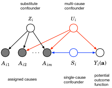
Figure 1: A graphical model argument for the deconfounder. The punchline is that if $Z_{i}$ renders the $A_{ij}$’s conditionally independent then there cannot be a multi-cause confounder. The proof is by contradiction. Assume conditional independence holds, $p(a_{i1},\ldots,a_{im}\,|\,z_{i})=\prod_{j}p(a_{ij}\,|\,z_{i})$; if there exists a multi-cause confounder $U_{i}$ (red) then, by $d$-separation, conditional independence cannot hold (pearl1988probabilistic). Note we cannot rule out the single-cause confounder $S_{i}$ (blue).

The graphical model in Figure 1 justifies the deconfounder and reveals its assumptions. Suppose we observe a $Z_{i}$ such that the conditional independence in Equation 5 holds. Further suppose there exists an unobserved multi-cause confounder $U_{i}$ (illustrated in red), which connects to multiple assigned causes and the outcome. If such a $U_{i}$ exists then the causes would be dependent, even conditional on $Z_{i}$. (This fact comes from $d$-separation.) But such dependence leads to a contradiction, that Equation 5 does not hold. Thus $U_{i}$ cannot exist.

There is a nuance. The conditional independence in Equation 5 cannot rule out the existence of an unobserved single-cause confounder, denoted $S_{i}$ in Figure 1. Even if such a confounder exists, the conditional independence still holds.

Here is the punchline. If we find a factor model that captures the population distribution of assigned causes then we have essentially discovered a variable that captures all multiple-cause confounders. The reason is that multiple-cause confounders induce dependence among the assigned causes, regardless of how they connect to the potential outcome function. Modeling their dependence, for which we have observations, provides a way to estimate variables that capture those confounders. This is the blessing of multiple causes.

2.3 The identification strategy of the deconfounder

How does the deconfounder identify potential outcomes? The classical strategy for causal identification is that ignorability, together with stable unit treatment value assumption (sutva) and overlap, identifies the potential outcomes (imbens2000role; hirano2004propensity; imai2004causal). The deconfounder continues to assume sutva and overlap, but it weakens the ignorability assumption.

Roughly, ignorability requires that there are no unobserved confounders. To weaken this assumption, the deconfounder constructs a substitute confounder that captures all multiple-cause confounders. (The proof is in Section 4.) Uncovering multi-cause confounders from data weakens the ignorability assumption to one of no unobserved single-cause confounders.

Thus the deconfounder relies on three assumptions: (1) sutva (rubin1980randomization; rubin1990comment); (2) no unobserved single-cause confounders; (3) overlap (imai2004causal).

Stable unit treatment value assumption (sutva).  The sutva requires that the potential outcomes of one individual are independent of the assigned causes of another individual. It assumes that there is no interference between individuals and there is only a single version of each assigned cause. See rubin1980randomization; rubin1990comment and Imbens:2015 for discussion.

No unobserved single-cause confounders.  Denote $X_{i}$ as the observed covariates. (Observed covariates are not necessarily confounders.) “No unobserved single-cause confounders” requires

$$A_{ij}\mathchoice{\mathrel{\hbox to0.0pt{$\displaystyle\perp$\hss}\mkern 2.0mu{\displaystyle\perp}}}{\mathrel{\hbox to0.0pt{$\textstyle\perp$\hss}\mkern 2.0mu{\textstyle\perp}}}{\mathrel{\hbox to0.0pt{$\scriptstyle\perp$\hss}\mkern 2.0mu{\scriptstyle\perp}}}{\mathrel{\hbox to0.0pt{$\scriptscriptstyle\perp$\hss}\mkern 2.0mu{\scriptscriptstyle\perp}}}Y_{i}(\mathbf{\boldsymbol{a}})\,|\,X_{i},\qquad j=1,\ldots,m.$$ (6)

We call this assumption “single ignorability.” Single ignorability differs from classical ignorability by only requiring marginal independence between individual causes $A_{ij}$ and the potential outcome $Y_{i}(\mathbf{\boldsymbol{a}})$. In contrast, classical ignorability requires $(A_{i1},\ldots,A_{im})\mathchoice{\mathrel{\hbox to0.0pt{$\displaystyle\perp$\hss}\mkern 2.0mu{\displaystyle\perp}}}{\mathrel{\hbox to0.0pt{$\textstyle\perp$\hss}\mkern 2.0mu{\textstyle\perp}}}{\mathrel{\hbox to0.0pt{$\scriptstyle\perp$\hss}\mkern 2.0mu{\scriptstyle\perp}}}{\mathrel{\hbox to0.0pt{$\scriptscriptstyle\perp$\hss}\mkern 2.0mu{\scriptscriptstyle\perp}}}Y_{i}(\mathbf{\boldsymbol{a}})\,|\,X_{i}$, i.e., the joint independence between the causes $(A_{i1},\ldots,A_{im})$ and the potential outcome function $Y_{i}(\mathbf{\boldsymbol{a}})$.

Roughly, single ignorability implies that we observe any confounders that affect only one of the causes; see Figure 1. This assumption is weaker than classical ignorability; we no longer need to observe all confounders. That said, whether the assumption is plausible depends on the particulars of the problem. Note that single ignorability reduces to the classical ignorability assumption when there is only one cause; both requires $\mathbf{\boldsymbol{A}}_{i}\mathchoice{\mathrel{\hbox to0.0pt{$\displaystyle\perp$\hss}\mkern 2.0mu{\displaystyle\perp}}}{\mathrel{\hbox to0.0pt{$\textstyle\perp$\hss}\mkern 2.0mu{\textstyle\perp}}}{\mathrel{\hbox to0.0pt{$\scriptstyle\perp$\hss}\mkern 2.0mu{\scriptstyle\perp}}}{\mathrel{\hbox to0.0pt{$\scriptscriptstyle\perp$\hss}\mkern 2.0mu{\scriptscriptstyle\perp}}}Y_{i}(\mathbf{\boldsymbol{a}})\,|\,X_{i}$, where $\mathbf{\boldsymbol{A}}_{i}$ and $\mathbf{\boldsymbol{a}}$ are one-dimensional.

When might single ignorability be plausible? Consider the movie-actor example. One possible confounder is the reputation of the director. Famous directors have access to a circle of capable actors; they also tend to make good movies with large revenues. If the dataset contains many actors, it is likely that several are in the circle of capable actors; the director’s reputation is a multi-cause confounder. (If only one actor in the dataset is capable then the director’s reputation is a single-cause confounder.)

Or consider the gwas problem. If a confounder affects SNPs—and we observe 100,000 SNPs per individual—then the confounder may be unlikely to have an effect on only one. The same reasoning can apply to other settings—medications in medical informatics data, neurons in neuroscience recordings, and vocabulary terms in text data.

By the same token, single ignorability may not be satisfied when there are very few assigned causes. Consider the neuroscience problem of inferring the relationship between brain activity and animal behavior, but where the scientist only records the activity of a small number of neurons. While unlikely that a confounder affects only one neuron in the brain, it may be more possible that a confounder affects only one of the observed neurons.

In domains where single ignorability is likely not satisfied, we suggest performing sensitivity analysis (robins2000sensitivity; gilbert2003sensitivity; imai2004causal) on the deconfounder estimates. It assesses the robustness of the estimate against unobserved single-cause confounding. In the context of gwas, Section 3.2 will illustrate the effect of violating single ignorability.

Overlap.   The final assumption of the deconfounder is that the substitute confounder $Z_{i}$ satisfies the overlap condition

$$p(A_{ij}\in\mathcal{A}\,|\,Z_{i})>0\text{ for all sets }\mathcal{A}\text{ with positive measure, i.e. }p(\mathcal{A})>0.$$ (7)

Overlap asserts that, given the substitute confounder, the conditional probability of any vector of assigned causes is positive. This assumption is sometimes stated as the second half of ignorability (imai2004causal).

The potential outcome $Y_{i}(\mathbf{\boldsymbol{a}})$ is not identifiable if the substitute confounder does not satisfy overlap. When the overlap is limited, i.e. $p(A_{ij}\in\mathcal{A}\,|\,Z_{i})$ is small for all values of $Z_{i}$, then the deconfounder estimates of the potential outcome $Y_{i}(\mathbf{\boldsymbol{a}})$ will have high variance.

For many probabilistic factor models, the overlap condition is satisfied. For example, probabilistic PCA assumes $A_{ij}\,|\,Z_{i}\sim\mathcal{N}(Z_{i}^{\top}\theta_{j},\sigma^{2})$. The normal distribution has support over the real line, which ensures $P(A_{ij}\in\mathcal{A}\,|\,Z_{i})>0$ for all $\mathcal{A}$ with positive measure. That said, as the dimensionality of $Z_{i}$ increases, overlap often becomes increasingly limited (d2017overlap). For example, probabilistic PCA returns increasingly small $\sigma^{2}$, which signals $P(A_{ij}\in\mathcal{A}\,|\,Z_{i})$ is small.

We can enforce overlap by constraining the allowable family of factor models. With continuous causes, we restrict to models with continuous densities on $\mathbb{R}$. (We assume the causes are full-rank, i.e., that no two causes are measurable with each other; if such a pair exists, merge them into a single cause.) With discrete causes, we restrict to factor models with support on the whole $\mathcal{A}$ and a $Z_{i}$ lower-dimensional than the causes.

Alternatively, we can merge highly correlated causes as a preprocessing step. For example, consider two causes—paracetamol and ibuprofen–that are always assigned the same value. We can merge them into one cause: we only estimate the potential outcome of either taking both drugs or taking neither. This merging step prevents the deconfounder from extrapolating for the assigned causes which the data carries little evidence. We can also resort to classical strategies of causal inference under limited overlap, for example subsampling the population (crump2009dealing).

How can we assess the overlap with respect to the substitute confounder? With a fitted factor model, we can analyze the conditional distribution of the assigned causes given the substitute confounder $P(A_{ij}\,|\,Z_{i})$ for all individual $i$’s. A conditional with low variance or low entropy signals limited overlap and the possibility of high-variance causal estimates.

We have described the main assumptions of the deconfounder. With sutva, overlap, and single ignorability, the deconfounder estimate is unbiased.

The deconfounder (informal version of Theorem 6). Assume sutva, single ignorability (Equation 6), and overlap (Equation 7). Then the deconfounder provides an unbiased estimate of the average causal effect:

$$\mathbb{E}_{Y}\left[Y_{i}(a_{1},\ldots,a_{m})\right]-\mathbb{E}_{Y}\left[Y_{i}(a^{\prime}_{1},\ldots,a^{\prime}_{m})\right]$$ (8)

$$= \mathbb{E}_{X,Z}\left[\mathbb{E}_{Y}\left[Y_{i}\,|\,A_{i1}=a_{1},\ldots,A_{im}=a_{m},X_{i},Z_{i}\right]\right]$$

$$-\mathbb{E}_{X,Z}\left[\mathbb{E}_{Y}\left[Y_{i}\,|\,A_{i1}=a^{\prime}_{1},\ldots,A_{im}=a^{\prime}_{m},X_{i},Z_{i}\right]\right],$$ (9)

where $Z_{i}$ denotes the substitute confounder constructed from the factor model.

The theorem relies on two properties of the substitute confounder: (1) it captures all multi-cause confounders; (2) it does not capture mediators. By its construction from probabilistic factor models, the substitute confounder captures all multi-cause confounders; again, see the graphical model argument in Figure 1. Moreover, the substitute confounder is constructed with only the observed causes; no outcome information is used and so it cannot pick up any mediators. Thus, along with single ignorability and overlap, the substitute confounder provides full ignorability. With ignorability in hand, treat the substitute confounder as if it were observed covariates and Equation 9 follows from a classical conditional independence argument (rosenbaum1983central). Section 4 discusses and proves this theorem (Theorem 6).

2.4 Practical details of the deconfounder

We next attend to some of the practical details of the deconfounder. The ingredients of the deconfounder are (1) a factor model of assigned causes, (2) a way to check that the factor model captures their population distribution, and (3) a way to estimate the conditional expectation $\mathbb{E}\left[Y_{i}(\mathbf{\boldsymbol{a}})\,|\,\hat{Z}_{i},\mathbf{\boldsymbol{A}}_{i}=\mathbf{\boldsymbol{a}}\right]$ for performing causal inference. We discuss each ingredient below (Section 2.4.1 and Section 2.4.2) and then describe the full deconfounder algorithm (Section 2.4.3). We connect the deconfounder to existing methods in the research literature (Section 2.5) and answer questions that may come up for the reader (Section 2.6).

2.4.1 Using the assignment model to infer a substitute confounder

The first ingredient is a factor model of the assigned causes, as defined in Equation 4, which we call the assignment model. Many models fall into this category, such as mixture models, mixed-membership models, and deep generative models. Each of these models can be written as Equation 4; they each involve a per-datapoint latent variable $Z_{i}$ and a per-cause parameter $\theta_{j}$. Fitting the factor model gives an estimate of the parameters $\theta_{j},j=1,\ldots,m$. When the fitted factor model captures the population distribution of the assigned causes then inferences about $Z_{i}$ can be used as substitute confounders in a downstream causal inference.

Example factor models.  The deconfounder requires that the investigator find an adequate factor model of the assigned causes and then use the factor model to estimate the posterior $p(z_{i}\,|\,\mathbf{\boldsymbol{a}}_{i})$. In the simulations and studies of Section 3, we will explore several classes of factor models; we describe some of them here.

One of the most common factor models is principal component analysis (pca). pca is appropriate when the assigned causes are real-valued. In its probabilistic form (tipping1999probabilistic), both $z_{i}$ and the per-cause parameters $\theta_{j}$ are real-valued $K$-vectors. The model is

$$\begin{split}Z_{ik}&\sim\mathcal{N}(0,\lambda^{2}),\quad k=1,\ldots,K,\\ A_{ij}\,|\,Z_{i}&\sim\mathcal{N}\left(z_{i}^{\top}\theta_{j},\sigma^{2}\right),\quad j=1,\ldots,m.\end{split}$$ (10)

We can fit probabilistic pca with maximum likelihood (or Bayesian methods) and use standard conditional probability to calculate $p(z_{i}\,|\,\mathbf{\boldsymbol{a}}_{i})$. Exponential family extensions of pca are also factor models (collins2002generalization; mohamed2009bayesian) as are some deep generative models (tran2017deep), which can be interpreted as a nonlinear probabilistic PCA.

When the assigned causes are counts then Poisson factorization (pf) is an appropriate factor model (schmidt2009bayesian; cemgil2009bayesian; gopalan2015scalable). pf is a probabilistic form of nonnegative matrix factorization (lee1999learning; lee2001algorithms), where $z_{i}$ and $\theta_{j}$ are positive $K$-vectors. The model is

$$\begin{split}Z_{ik}&\sim\textrm{Gamma}(\alpha_{0},\alpha_{1}),\quad k=1,\ldots,K,\\ A_{ij}\,|\,Z_{i}&\sim\textrm{Poisson}(z_{i}^{\top}\theta_{j}),\quad j=1,\ldots,m.\end{split}$$ (11)

pf can be fit to large datasets with efficient variational methods (gopalan2015scalable). In general, the deconfounder can use variational methods, or other forms of approximate inference, to estimate $p(z_{i}\,|\,\mathbf{\boldsymbol{a}}_{i})$.

A final example of a factor model is the deep exponential family (def) (ranganath2015deep). A def is a probabilistic deep neural network. It uses exponential families to generalize classical models like the sigmoid belief network (neal1990learning) and deep Gaussian models (rezende2014stochastic). For example, a two-layer def models each observation as

$$\begin{split}Z_{2,il}&\sim\textrm{Exp-Fam}_{2}(\alpha),\quad l=1,\ldots,L,\\ Z_{1,ik}\,|\,Z_{2,i}&\sim\textrm{Exp-Fam}_{1}(g_{1}(z_{2,i}^{\top}\theta_{1,k})),\quad k=1,\ldots,K,\\ A_{ij}\,|\,Z_{1,i}&\sim\textrm{Exp-Fam}_{0}(g_{0}(z_{1,i}^{\top}\theta_{0,j})),\quad j=1,\ldots,m.\end{split}$$ (12)

Here Exp-Fam is an exponential family distribution, $\theta_{*}$ are parameters, and $g_{*}(\cdot)$ are link functions. Each layer of the def is a generalized linear model (mccullagh2018generalized; mccullagh1989generalized). The def inherits the flexibility of deep neural networks, but uses exponential families to capture different types of layered representations and data. For example, if the assigned causes are counts then $\textrm{Expfam}_{0}$ can be Poisson; if they are reals then it can be Gaussian. Approximate inference in def can be performed with black box variational methods (ranganath2014black).

Predictive checks for the assignment model.  The deconfounder requires that its factor model captures the population distribution of the assigned causes. To assess the fidelity of the chosen model, we use predictive checks. A predictive check compares the observed assignments with the assignments that would have been observed under the model.

First hold out a subset of assigned causes for each individual $a_{i\ell}$, where $\ell$ indexes some held-out causes. The heldout assignments are written $\mathbf{\boldsymbol{a}}_{i,\textrm{held}}$ and note we hold out randomly selected causes for each individual. The observed assignments are written $\mathbf{\boldsymbol{a}}_{i,\textrm{obs}}$.

Next fit the factor model to the remaining assignment data $\mathcal{D}=\{\mathbf{\boldsymbol{a}}_{i,\textrm{obs}}\}_{i=1}^{n}$. This results in a fitted assignment model $p(z,\theta\,|\,\mathbf{\boldsymbol{a}})$. For each individual $i$, calculate the local posterior distribution of $p(z_{i}\,|\,\mathbf{\boldsymbol{a}}_{i,\textrm{obs}})$.

Here is the predictive check. First sample values for the held-out causes from their predictive distribution,

$$p(\mathbf{\boldsymbol{a}}_{i,\textrm{held}}^{\textrm{rep}}\,|\,\mathbf{\boldsymbol{a}}_{i,\textrm{obs}})=\int p(\mathbf{\boldsymbol{a}}_{i,\textrm{held}}\,|\,z_{i})p(z_{i}\,|\,\mathbf{\boldsymbol{a}}_{i,\textrm{obs}})\mathop{}\!\mathrm{d}z_{i}.$$ (13)

This distribution integrates out the local posterior $p(z_{i}\,|\,\mathbf{\boldsymbol{a}}_{i,\textrm{obs}})$. (An approximate posterior also suffices; we discuss why in Section 2.6.5.)

Then compare the replicated data to the held-out data. To compare, calculate the expected log probability

$$t(\mathbf{\boldsymbol{a}}_{i,\textrm{held}})=\mathbb{E}_{Z}\left[\log p(\mathbf{\boldsymbol{a}}_{i,\textrm{held}}\,|\,Z)\,|\,\mathbf{\boldsymbol{a}}_{i,\textrm{obs}}\right],$$ (14)

which relates to their marginal log likelihood. In the nomenclature of posterior predictive checks, this is the “discrepancy function” that we use; one can use others.

Finally calculate the predictive score,

$$\text{predictive score}=p\left(t(\mathbf{\boldsymbol{a}}_{i,\textrm{held}}^{\textrm{rep}})<t(\mathbf{\boldsymbol{a}}_{i,\textrm{held}})\right).$$ (15)

Here the randomness stems from $\mathbf{\boldsymbol{a}}_{i,\textrm{held}}^{\textrm{rep}}$ coming from the predictive distribution in Equation 13, and we approximate the predictive score with Monte Carlo.

How to interpret the predictive score? A good model will produce values of the held-out causes that give similar log likelihoods to their real values—the predictive score will not be extreme. A mismatched model will produce an extremely small predictive score, often where the replicated data has much higher log likelihood than the real data. An ideal predictive score is around 0.5. We consider predictive scores with predictive scores larger than 0.1 to be satisfactory; we do not have enough evidence to conclude significant mismatch of the assignment model. Note that the threshold of 0.1 is a subjective design choice. We find such assignment models that pass this threshold often yield satisfactory causal estimates in practice. Figure 2 illustrates a predictive check of a good assignment model. Section 3 shows predictive checks in action.

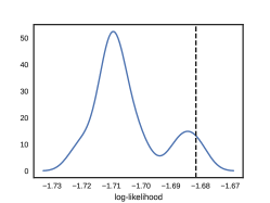
Figure 2: Predictive checks for the assignment model. The vertical dashed line shows $t(\mathbf{\boldsymbol{a}}_{i,\textrm{held}})$. The blue curve shows the kde of $t(\mathbf{\boldsymbol{a}}_{i,\textrm{held}}^{\textrm{rep}})$. The predictive score is the area under the blue curve to the left of the vertical dashed line. The predictive score of this assignment model is larger than 0.1; we consider it satisfactory.

Predictive checks blend a circle of related ideas around posterior predictive checks (ppcs) (Rubin:1984), ppcs with realized discrepancies (Gelman:1996), ppcs with held-out data (Gelfand:1992), and stage-wise checking of hierarchical models (Dey:1998; Bayarri:2007). They also relate to Bayesian causal model criticism (tran2016model) and ppcs in genome-wide association studies (gwas) (mimno2015posterior). Finding, fitting, and checking the factor model also relates to the Box’s loop in Bayesian data analysis (blei2014build; gelman2013bayesian).

2.4.2 The outcome model

We described how to fit and check a factor model of multiple assigned causes. We now discuss how to fold in the observed outcomes and to use the fitted factor model to correct for unobserved confounders.

Suppose $p(z_{i}\,|\,\mathbf{\boldsymbol{a}}_{i},\mathcal{D})$ concentrates around a point $\hat{z}_{i}$. Then we can use $\hat{z}_{i}$ as a confounder. Follow Section 2.1 to calculate the iterated expectation on the left side of Equation 2. However, replace the observed confounders with the substitute confounder; the goal is to calculate $\mathbb{E}\left[\mathbb{E}\left[Y_{i}(\mathbf{\boldsymbol{a}})\,|\,\mathbf{\boldsymbol{A}}_{i}=\mathbf{\boldsymbol{a}},Z_{i}\right]\right]$. First, approximate the outside expectation with Monte Carlo,

$$\mathbb{E}\left[\mathbb{E}\left[Y_{i}(\mathbf{\boldsymbol{a}})\,|\,\mathbf{\boldsymbol{A}}_{i}=\mathbf{\boldsymbol{a}},Z_{i}\right]\right]\approx\frac{1}{n}\sum_{i=1}^{n}\mathbb{E}_{Y}\left[Y_{i}(\mathbf{\boldsymbol{A}}_{i})\,|\,\mathbf{\boldsymbol{A}}_{i}=\mathbf{\boldsymbol{a}},Z_{i}=\hat{z}_{i}\right].$$ (16)

This approximation uses the substitute confounder $\hat{z}_{i}$, integrating over its population distribution. It uses the model to infer the substitute confounder from each data point and then integrates the distribution of that inferred variable induced by the population distribution of data.

Turn now to the inner expectation of Equation 16. We fit a function to estimate this quantity,

$$\mathbb{E}\left[Y_{i}(\mathbf{\boldsymbol{A}}_{i})\,|\,\mathbf{\boldsymbol{A}}_{i}=\mathbf{\boldsymbol{a}},Z_{i}=z\right]=f(\mathbf{\boldsymbol{a}},z).$$ (17)

The function $f(\mathbf{\boldsymbol{a}},z)$ is called the outcome model and can be fit from the augmented observed data $\{\mathbf{\boldsymbol{a}}_{i},\hat{z}_{i},y_{i}(\mathbf{\boldsymbol{a}}_{i})\}$. For example, we can minimize their discrepancy via some loss function $\ell$:

$$\hat{f}=\operatorname*{arg\,min}_{f}\sum^{n}_{i=1}\ell(y_{i}(\mathbf{\boldsymbol{a}}_{i})-f(\mathbf{\boldsymbol{a}}_{i},\hat{z}_{i})).$$

Like the factor model, we can check the outcome model—it is fit to observed data and should be predictive of held-out observed data (tran2016model).

One outcome model we consider is a simple linear function,

$$f(\mathbf{\boldsymbol{a}},z)=\beta^{\top}\mathbf{\boldsymbol{a}}+\gamma^{\top}z.$$ (18)

Another outcome model we consider is where $f(\cdot)$ is linear in the assigned causes $\mathbf{\boldsymbol{a}}$ and the “reconstructed assigned causes” $\hat{\mathbf{\boldsymbol{a}}}(z)=\mathbb{E}_{M}\left[\mathbf{\boldsymbol{A}}\,|\,z\right]$, an expectation from the fitted factor model. This class of functions is

$$f(\mathbf{\boldsymbol{a}},z)=\beta^{\top}\mathbf{\boldsymbol{a}}+\gamma^{\top}\hat{\mathbf{\boldsymbol{a}}}(z).$$ (19)

This outcome model relates to the generalized propensity score (imbens2000role; hirano2004propensity). Equation 19 can be seen as using $\hat{a}(z)$ as a proxy for the propensity score, a substitution that is used in Bayesian statistics (laird1982approximate; tierney1986accurate; geisser1990validity); this substitution is justified when higher moments of the assignment are similar across individuals. In both models, the coefficient $\beta$ represents the average causal effect of raising each cause by one individual.

But we are not restricted to linear models. Other outcome models like random forests (wager2017estimation) and Bayesian additive regression trees (hill2011bayesian) all apply here.

Note that devising an outcome model is just one approach to approximating the inner expectation of Equation 16. Another approach is again to use Monte Carlo. There are several possibilities. In one, group the confounder $\hat{z}_{i}$ into bins and approximate the expectation within each bin. In another, bin by the propensity score $p(a_{i}\,|\,\hat{z}_{i})$ and approximate the inner expectation within each propensity-score bin (rosenbaum1983central; lunceford2004stratification). A third possibility—if the assigned causes are discrete and the number of causes is small—is to use the propensity score with inverse propensity weighting (horvitz1952generalization; rosenbaum1983central; heckman1998characterizing; dehejia2002propensity).

2.4.3 The full algorithm, and an example

We described each component of the deconfounder. Algorithm 1 gives the full algorithm, a procedure for estimating Equation 16. The steps are: (1) find, fit, and check a factor model to the dataset of assigned causes; (2) estimate $\hat{z}_{i}$ for each datapoint; (3) find and fit a outcome model; (4) use the outcome model and estimated $\hat{z}_{i}$ to do causal inference.

Input: a dataset of assigned causes and outcomes $\{(\mathbf{\boldsymbol{a}}_{i},y_{i})\},\,\,i=1,\ldots,n$

Output: the average potential outcome $\mathbb{E}\left[Y(\mathbf{\boldsymbol{a}})\right]$ for any causes $\mathbf{\boldsymbol{a}}$

repeat

       choose an assignment model from the class in Equation 4

       fit the model to the assigned causes $\{\mathbf{\boldsymbol{a}}_{i}\},\,\,i=1,\ldots,n$

       check the fitted model $\hat{M}$

      

until the assignment check is satisfactory

foreach datapoint $i$ do

       calculate $\hat{z}_{i}=\mathbb{E}_{\hat{M}}\left[Z_{i}\,|\,\mathbf{\boldsymbol{a}}_{i}\right]$.

end foreach

repeat

       choose an outcome model from Equation 17

       fit the outcome model to the augmented dataset $\{(\mathbf{\boldsymbol{a}}_{i},y_{i},\hat{z}_{i})\},\,\,i=1,\ldots,n$

       check the fitted outcome model

      

until the outcome check is satisfactory

estimate the average causal effect $\mathbb{E}\left[Y(\mathbf{\boldsymbol{a}})\right]-\mathbb{E}\left[Y(\mathbf{\boldsymbol{a}}^{\prime})\right]$ by Equation 16

Algorithm 1 The Deconfounder

Example.  Consider a causal inference problem in genome-wide association studies (gwas) (stephens2009bayesian; visscher201710): how do human genes causally affect height? Here we give a brief account of how to use the deconfounder, omitting many of the details. We analyze gwas problems extensively in Section 3.2.

Consider a dataset of $n=5,000$ individuals; for each individual, we measure height and genotype, specifically the alleles at $m=100,000$ locations, called the single-nucleotide polymorphisms (snps). Each snp is represented by a count of 0, 1, or 2; it encodes how many of the individual’s two nucleotides differ from the most common pair of nucleotides at the location. Table 2 illustrates a snippet of the data (10 individuals).

ID $(i)$	SNP_1 $(a_{i,1})$	SNP_2 $(a_{i,2})$	SNP_3 $(a_{i,3})$	SNP_4 $(a_{i,4})$	SNP_5 $(a_{i,5})$	SNP_6 $(a_{i,6})$	SNP_7 $(a_{i,7})$	SNP_8 $(a_{i,8})$	SNP_9 $(a_{i,9})$	$\cdots$	SNP_100K $(a_{i,100K})$	Height (feet) $(y_{i})$
1	1	0	0	1	0	0	1	2	0	$\cdots$	0	5.73
2	1	2	2	1	2	1	1	0	1	$\cdots$	2	5.26
3	2	0	1	1	0	1	0	1	1	$\cdots$	2	6.24
4	0	0	0	1	1	0	1	2	0	$\cdots$	0	5.78
5	1	2	1	1	1	0	1	0	0	$\cdots$	1	5.09
$\vdots$						$\vdots$						$\vdots$

Table 2: How do SNPs causally affect height? This table shows a portion of a dataset: simulated SNPs as the multiple causes and height as the outcome.

We simulate such a dataset of genotypes and height. We generate each individual’s genotypes by simulating heterogeneous mixing of populations (pritchard2000association). We then generate the height from a linear model of the snp s (i.e. the assigned causes) and some simulated confounders. (The confounders are only used to simulate data; when running the deconfounder, the confounders are unobserved.) In this simulated data, the coefficients of the SNPs are the true causal effects; we denote them $\beta^{*}=(\beta^{*}_{1},\ldots,\beta^{*}_{m})$. See Section 3.2 for more details of the simulation.

The goal is to infer how the snp s causally affect human height, even in the presence of unobserved confounders. The $m$-dimensional snp vector $\mathbf{\boldsymbol{a}}_{i}=(a_{i1},a_{i2},...,a_{im})$ is the vector of assigned causes for individual $i$; the height $y_{i}$ is the outcome. We want to estimate the potential outcome: what would the (average) height be if we set a person’s snp to be $\mathbf{\boldsymbol{a}}=(a_{1},a_{2},...,a_{m})$? Mathematically, this is the average potential outcome function: $\mathbb{E}[Y_{i}(\mathbf{\boldsymbol{a}})]$, where the vector of assigned causes $\mathbf{\boldsymbol{a}}$ takes values in $\{0,1,2\}^{m}$.

We apply the deconfounder: model the assigned causes, infer a substitute confounder, and perform causal inference. To infer a substitute confounder, we fit a factor model of the assigned causes. Here we fit a $50$-factor pf model, as in Equation 11. This fit results in estimates of non-negative factors $\hat{\theta}_{j}$ for each assigned cause (a $K$-vector) and non-negative weights $\hat{z}_{i}$ for each individual (also a $K$-vector).

If the predictive check greenlights this fit, then we take the posterior predictive mean of the assigned causes as the reconstructed assignments, $\hat{a}_{j}(z_{i})=\hat{z}_{i}^{\top}\hat{\theta}_{j}$. For brevity, we do not report the predictive check here. (The model passes.) We demonstrate predictive checks for gwas in the empirical studies of Section 3.2.

Using the reconstructed assigned causes, we estimate the average potential outcome function. Here we fit a linear outcome model to the height $y_{i}$ against both of the assigned causes $\mathbf{\boldsymbol{a}}_{i}$ and reconstructed assignment $\hat{\mathbf{\boldsymbol{a}}}(z_{i})$,

$$y_{i}\sim\mathcal{N}\left(\beta_{0}+\beta^{\top}\mathbf{\boldsymbol{a}}_{i}+\gamma^{\top}\hat{\mathbf{\boldsymbol{a}}}(z_{i}),\sigma^{2}\right).$$ (20)

This regression is high dimensional $(m>n)$; for regularization, we use an $L_{2}$-penalty on $\beta$ and $\gamma$ (equivalently, normal priors). Fitting the outcome model gives an estimate of regression coefficients $\{\hat{\beta}_{0},\hat{\beta},\hat{\gamma}\}$. Because we use a linear outcome model, the regression coefficients $\hat{\beta}$ estimate the true causal effect $\beta^{*}$.

Table 3 evaluates the causal estimates obtained with and without the deconfounder. We focus on the root mean squred error (rmse) of $\hat{\beta}$ to $\beta^{*}$. (“Causal estimation without the deconfounder” means fitting a linear model of the height $y_{i}$ against the assigned causes $\mathbf{\boldsymbol{a}}_{i}$.) The deconfounder produces closer-to-truth causal estimates.

	w/o deconfounder	w/ deconfounder
RMSE$\times 10^{-2}$	49.6	41.2

Table 3: Rmse of the causal coefficients $\hat{\beta}$ with and without the deconfounder in a GWAS simulation study. We treat this rmse as a metric of how close the estimated potential outcome function is to the truth. In this toy problem, the deconfounder produces closer-to-truth causal estimates.

2.5 Connections to genome-wide association studies

Many methods from the research literature, especially around genome-wide association studies, can be reinterpreted as instances of the deconfounder algorithm. Each can be seen as positing a factor model of assigned causes (Section 2.4.1) and a conditional outcome model (Section 2.4.2).

The deconfounder justifies each of these methods as forms of multiple causal inference and, though predictive checks, points to how a researcher can usefully compare and assess them. Most of these methods were motivated by imagining true unobserved confounding structure. However, the theory around the deconfounder shows that a well-fitted factor model will capture confounders independent of a researcher imagining what they may be; see the question in Section 2.6.5.

Below we describe many methods from the gwas literature and show how they can be viewed as deconfounder algorithms. The gwas problem is described in Section 2.4.3.

Linear mixed models.  The linear mixed model (lmm) is one the most popular classes of methods for analyzing GWAS (yu2006unified; kang2008efficient; yang2014advantages; lippert2011fast; loh2015efficient; JMLR:v18:15-143). Seen through the lens of the deconfounder, an lmm posits a linear outcome model that depends on both the SNPs and a scalar latent factor $Z_{i}$.

In the lmm literature, $Z_{i}$ is not explicitly drawn from a factor model; rather, $Z_{1:n}$ are from a multivariate Gaussian whose covariance matrix, called the “kinship matrix,” is calculated from the observed SNPs $\mathbf{\boldsymbol{a}}_{1:n}$. However, this is mathematically equivalent to posterior latent factors from a one-dimensional pca model. Subject to its capturing the distribution of SNPs, the lmm is performing multiple causal inference with a deconfounder.

Principal component analysis.  A related approach is to first perform (multi-dimensional) pca on the SNP matrix and then to estimate an outcome model from the corresponding residuals (price2006principal). This too is an instance of the deconfounder. As a factor model, pca is described in Equation 10. Fitting an outcome model to its residuals is equivalent to conditioning on the reconstructed assignments, Equation 19.

Logistic factor analysis.  Closely related to pca is logistic factor analysis (lfa) (song2015testing; hao2015probabilistic). lfa can be seen as the following factor model,

$$\begin{split}Z_{i}&\sim\mathcal{N}(0,I)\\ \pi_{ij}\,|\,Z_{i}&\sim\mathcal{N}(z_{i}^{\top}\theta_{j},\sigma^{2}),\quad j=1,\ldots,m,\\ A_{ij}\,|\,\pi_{ij}&\sim\textrm{Binomial}(2,\textrm{logit}^{-1}(\pi_{ij})),\quad j=1,\ldots,m.\end{split}$$

If it captures the SNP matrix well, then $Z_{i}$ can be viewed as a substitute confounder.

With lfa in hand, song2015testing use inverse regression to perform association tests. Their approach is equivalent to assuming an outcome model conditional on the reconstructed assignments $a(\hat{z}_{i})$, again Equation 19, and subsequently testing for non-zero coefficients.

In a variant of lfa, tran2017implicit use a neural-network based model of the unobserved confounder, connecting this model to a causal inference with a nonparametric structural equation model (Pearl:2009a). They take an explicitly causal view of the testing problem.

Mixed-membership models.  Finally, many statistical geneticists use mixed-membership models (Airoldi:2014) to capture the latent population structure of SNPs, and then condition on that structure in downstream analyses (pritchard2000inference; pritchard2000association; falush2003inference; falush2007inference). In genetics, a mixed-membership model is a factor model that captures latent ancestral populations. The latent variable $Z_{i}$ is on the $K-1$ simplex; it represents how much individual $i$ reflects each ancestral population. The observed SNP $A_{ij}$ comes from a mixture of Binomials, where $Z_{i}$ determines its mixture proportions.

Using these models, researchers use a linear outcome model conditional on $z_{i}$ and devise tests for significant associations (pritchard2000association; song2015testing; tran2017implicit). The deconfounder justifies this practice from a causal perspective, and underlines the importance of finding a model of population structure that captures the per-individual distribution of SNPs.

2.6 A conversation with the reader

In this section, we answer some questions a reader might have.

2.6.1 Why do I need multiple causes?

The deconfounder uses latent variables to capture dependence among the assigned causes. The theory in Section 4 says that a latent variable which captures this dependence will contain all valid multi-cause confounders. But estimating this latent variable requires evidence for the dependence, and evidence for dependence cannot exist with just one assigned cause. Thus the deconfounder requires multiple causes.

2.6.2 Is the deconfounder free lunch?

The deconfounder is not free lunch—it trades confounding bias for estimation variance. Take an information point of view: the deconfounder uses a portion of information in the data to estimate a substitute confounder; then it uses the rest to estimate causal effects. By contrast, classical causal inference uses all the information to estimate causal effects, but it must assume ignorability. Put differently, while the deconfounder assumes the weaker assumption of single ignorability, it pays for this flexibility in the information it has available for causal estimation. Hence the deconfounder estimate often has higher variance.

Suppose full ignorability is satisfied. Then both classical causal inference and the deconfounder provide unbiased causal estimates, though the deconfounder will be less confident; it has higher variance. Now suppose only single ignorability is satisfied. The deconfounder still provides unbiased causal estimates, but classical causal inference is biased.

2.6.3 Why does the deconfounder have two stages?

Algorithm 1 first fits a factor model to the assigned causes and then fits the potential outcome function. This is a two stage procedure. Why? Can we fit these two models jointly?

One reason is convenience. Good models of assigned causes may be known in the research literature, such as for genetic studies. Moreover, separately fitting the assignment model allows the investigator to fit models to any available data of assigned causes, including datasets where the outcome is not measured.

Another reason for two stages is to ensure that $Z_{i}$ does not contain mediators, variables along the causal path between the assigned causes and the outcome. Intuitively, excluding the outcome ensures that the substitute confounders are “pre-treatment” variables; we cannot identify a mediator by looking only at the assigned causes. More formally, excluding the outcome ensures that the model satisfies $p(z_{i}\,|\,\mathbf{\boldsymbol{a}}_{i},y_{i}(\mathbf{\boldsymbol{a}}_{i}))=p(z_{i}\,|\,\mathbf{\boldsymbol{a}}_{i})$; this equality cannot hold if $Z_{i}$ contains a mediator.

2.6.4 How does the deconfounder relate to the generalized propensity score? What about instrumental variables?

The deconfounder relates to both.

The deconfounder can be interpreted as a generalized propensity score approach, except where the propensity score model involves latent variables. If we treat the substitute confounder $Z_{i}$ as observed covariates, then the factor model $P(A_{i}\,|\,Z_{i})$ is precisely the propensity score of the causes $A_{i}$. With this view, the innovation of the deconfounder is in $Z_{i}$ being latent. Moreover, it is the multiplicity of the causes $A_{i1},\ldots,A_{im}$ that makes a latent $Z_{i}$ feasible; we can construct $Z_{i}$ by finding a random variable that renders all the causes conditionally independent.

The deconfounder can also be interpreted as a way of constructing instruments using latent factor models. Think of a factor model of the causes with linearly separable noises: $A_{ij}\stackrel{{\scriptstyle a.s.}}{{=}}f(Z_{i})+\epsilon_{ij}$. Given the substitute confounder, consider the residual of the causes $\epsilon_{ij}$. Assuming single ignorability, the variable $\epsilon_{ij}$ is an instrumental variable for the $j$th cause $A_{ij}$. For example, with probabilistic pca the residual is ${\epsilon_{ij}=A_{ij}-Z_{i}^{\top}\theta_{j}}\sim\mathcal{N}(0,\sigma^{2})$.

The residual $\epsilon_{ij}$ satisfies the requirements of being an instrument for $A_{ij}$: (1) The residual $\epsilon_{ij}$ correlates with the cause $A_{ij}$. (2) The residual $\epsilon_{ij}$ affects the outcome only through the cause $A_{ij}$; this fact is true because the substitute confounder $Z_{i}$ is constructed without using any outcome information. (3) The residual $\epsilon_{ij}$ cannot be correlated with a confounder; this is true because $Z_{i}\perp\epsilon_{ij}$ by construction from the factor model, where $P(Z_{i})$ and $P(A_{ij}\,|\,Z_{i})$ are specified separately.

However, the deconfounder differs from classical instrumental variables approaches because it uses latent variable models to construct instruments, rather than requiring that instruments be observed. The latent variable construction is feasible because the multiplicity of the causes allows us to construct $Z_{i}$ and $\epsilon_{ij}$ from the conditional independence requirement.

2.6.5 Does the factor model of the assigned causes need to be the true assignment model? Which factor model should I choose if multiple factor models return good predictive scores?

Finding a good factor model is not the same as finding the “true” model of the assigned causes. We do not assume the inferred variable $Z_{i}$ reflects a real-world unobserved variable.

Rather, the deconfounder requires the factor model to capture the population distribution of the assigned causes and, more particularly, their dependence structure. This requirement is why predictive checking is important. If the deconfounder captures the population distribution—if the predictive check returns high predictive scores—then we can use the inferred local variables $Z_{i}$ as substitute confounders.

For the same reason, the deconfounder can rely on approximate inference methods to infer the substitute confounder. The predictive check evaluates whether $Z_{i}$ provides a good predictive distribution, regardless of how it was inferred. As long as the model and (approximate) inference method together give a good predictive distribution—one close to the population distribution of the assigned causes—then the downstream causal inference is valid. We use approximate inference for most of the factor models we study in Section 3.

Suppose multiple factor models give similarly good predictive scores in the predictive check. In this case, we recommend choosing the factor model with the lowest capacity. Factor models with similar predictive scores often result in causal estimates with similarly little bias. But the variance of these estimates can differ. Factor models with high capacity can compromise overlap and lead to high-variance estimates; factor models with low capacities tend to produce lower variance causal estimates. The empirical study in Section 3.1 demonstrates this phenomenon.

2.6.6 Can the causes be causally dependent among themselves?

When the causes are causally dependent, the deconfounder can still provide unbiased estimates of the potential outcomes. Its success relies on a valid substitute confounder.

Note there are cases where a valid substitute confounder cannot exist. For example, consider a cause $A_{1}$ that causally affects $A_{2}$ according to $A_{1}\sim\mathcal{N}(0,1),A_{2}=A_{1}+\epsilon,\epsilon\sim\mathcal{N}(0,1)$. In this case, a substitute confounder $Z$ must satisfy $Z\stackrel{{\scriptstyle a.s.}}{{=}}A_{1}$ or $Z\stackrel{{\scriptstyle a.s.}}{{=}}A_{2}$, because it needs to render the two causes conditionally independent. But such a $Z$ does not satisfy overlap.

On the other hand, causal dependence among the causes does not necessarily imply the nonexistence of a valid substitute confounder. Consider a different mechanism for the causal relationship between $A_{1}$ and $A_{2}$,

$$A_{1} \sim\mathcal{N}(0,1),$$

$$A_{2} =|A_{1}|+\epsilon,\quad\epsilon\sim\mathcal{N}(0,1).$$

Here $Z\stackrel{{\scriptstyle a.s}}{{=}}|A_{1}|$ is a valid substitute confounder; it satisfies overlap and renders $A_{1}$ conditionally independent of $A_{2}$.

Empirically, it is hard to detect the nonexistence of a valid substitute confounder without knowing the functional form of how the causes are structurally dependent. Insisting on using the deconfounder in this case results in limited overlap and high variance causal estimates downstream. We will illustrate this phenomenon in Section 3.1.

Finally, we recommend applying the deconfounder to non-causally dependent causes. A valid substitute confounder is guaranteed to exist in this case; it will both satisfy overlap and render the causes conditionally independent of each other.

2.6.7 Should I condition on known confounders and covariates?

Suppose we also observe known confounders and other covariates $X_{i}$. The deconfounder maintains its theoretical properties when we condition on observed covariates $X_{i}$ as well as infer a substitute confounder $Z_{i}$. In particular, if $X_{i}$ is “pre-treatment” —it does not include any mediators—then the causal estimate will be unbiased (imai2004causal) (also see Theorem 6 below). In general, it is good to condition on observed confounders, especially if they may contain single-cause confounders.

That said, we do not need to condition on observed confounders that affect more than one of the causes; it suffices to condition only on the substitute confounder $Z_{i}$. And there is a trade off. Conditioning on covariates $X_{i}$ maintains unbiasedness but it hurts efficiency. If the true causal effect size is small then large confidence or credible intervals will conclude these small effects as insignificant—inefficient causal estimates can bury the real causal effects. The empirical study in Section 3.1 explores this phenomenon.

2.6.8 How can I assess the uncertainty of the deconfounder?

The uncertainty in the deconfounder comes from two sources, the factor model and the outcome model. The deconfounder first fits (and checks) the factor model; it gives a substitute confounder $Z_{i}\sim p(z_{i}\,|\,\mathbf{\boldsymbol{a}}_{i})$. It then uses the mean of the substitute confounder $\hat{z}_{i}=\mathbb{E}_{\hat{M}}\left[Z_{i}\,|\,\mathbf{\boldsymbol{a}}_{i}\right]$ to fit an outcome model $p(y_{i}\,|\,\mathbf{\boldsymbol{a}}_{i},\hat{z}_{i})$ and compute the potential outcome estimate $\mathbb{E}\left[Y_{i}(\mathbf{\boldsymbol{a}})\right]$.

To assess the uncertainty of the deconfounder, we consider the uncertainty from both sources. We first draw $s$ samples $\{z_{i}^{(1)},\ldots,z_{i}^{(s)}\}$ of the substitute confounder: $z_{i}^{(l)}\stackrel{{\scriptstyle iid}}{{\sim}}p(z_{i}\,|\,\mathbf{\boldsymbol{a}}_{i}),l=1,\ldots,s$. For each sample $z_{i}^{(l)}$, we fit an outcome model and compute a point estimate of the potential outcome. (If the outcome model is probabilistic, we compute the posterior distribution of its parameters; this leads to a posterior of the potential outcome.) We aggregate the estimates of the potential outcome (or its distributions) from the $s$ samples $\{z_{i}^{(1)},\ldots,z_{i}^{(s)}\}$; the aggregated estimate is a collection of point estimates of the potential outcome (or a mixture of its posterior distributions). The variance of this aggregated estimate describes the uncertainty of the deconfounder; it reflects how the finite data informs the estimation of the potential outcome. In a two-cause smoking study, Section 3.1 illustrates this strategy for calculating the uncertainty of the deconfounder.

3 Empirical studies

We study the deconfounder in three empirical studies. Two studies involve simulations of realistic scenarios; these help assess how well the deconfounder performs relative to ground truth. In Section 3.1 we study semi-synthetic data about smoking; the causes are a real dataset about smoking and the effect (medical expenses) is simulated. In Section 3.2 we study semi-synthetic data about genetics. Finally, in Section 3.3 we study real data about actors and movie revenue; there is no simulation. All three of these studies demonstrate the benefits of the deconfounder. They show how predictive checks reveal potential issues with downstream causal inference and how the deconfounder can provide closer-to-truth causal estimates.

Each stage of the deconfounder requires computation: to fit the factor model, to check the factor model, to calculate the substitute deconfounder, and to fit the outcome model. In all these stages, we use black box variational inference (bbvi) (ranganath2014black) as implemented in Edward, a probabilistic programming system (tran2017deep; tran2016edward). (This was a choice; the deconfounder can be used with other methods for calculating the posterior and fitting models. For example, we can also use Stan (carpenter2017stan), which is a probabilistic programming language available in R (team2013r).)

3.1 Two causes: How smoking affects medical expenses

We first study the deconfounder with semi-synthetic data about smoking. The 1987 National Medical Expenditures Survey (NMES) collected data about smoking habits and medical expenses in a representative sample of the U.S. population (imai2004causal; nmes1987). The dataset contains 9,708 people and 8 variables about each. For each person, we focus on the current marital status ($a_{\textrm{mar}}$), the cumulative exposure to smoking ($a_{\textrm{exp}}$), and the last age of smoking ($a_{\textrm{age}}$). (We standardize all variables.)

A true outcome model and causal inference problem.  We use the assigned causes from the survey to simulate a dataset of medical expenses, which we will consider as the outcome variable. Our true model is linear,

$$y_{i}=\beta_{\textrm{mar}}\,a_{\textrm{mar},i}+\beta_{\textrm{exp}}\,a_{\textrm{exp},i}+\beta_{\textrm{age}}\,a_{\textrm{age},i}+\varepsilon_{i},$$ (21)

where $\varepsilon_{i}\sim\mathcal{N}(0,1)$. We generate the true causal coefficients from

$$\beta_{\textrm{mar}}\sim\mathcal{N}(0,1)\quad\beta_{\textrm{exp}}\sim\mathcal{N}(0,1)\quad\beta_{\textrm{age}}\sim\mathcal{N}(0,1).$$ (22)

and from these coefficients we generate the outcome for each individual. The result is a semi-synthetic dataset of 9,708 tuples $(a_{\textrm{mar},i},a_{\textrm{exp},i},a_{\textrm{age},i},y_{i})$. The assigned causes are from the real world, but we know the true outcome model. Note that the last smoking age is a multi-cause confounder—it affects both marital status and exposure and is one of the causes of the expenses.

We are interested in the causal effects of marital status and smoking exposure on medical expenses. But suppose we do not observe age; it is an unobserved confounder. We can use the deconfounder to solve the problem.

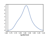
(a) Linear Model

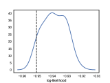
(b) Quadratic Model

Figure 3: Predictive checks for the substitute confounder $z$ obtained from a linear factor model (a) and a quadratic factor model (b). The blue line is the kde of the test-statistic based on the predictive distribution. The dashed vertical line shows the value of the test-statistic on the observed dataset. The figure shows that the linear model mismatches the data—the observed statistic falls in a low probability region of the kde. The quadratic factor model is a better fit to the data.

Modeling the assigned causes.  We begin by finding a good factor model of the assigned causes $(a_{\textrm{mar},i},a_{\exp,i})$. Because there are two observed assigned causes, we consider models with a single scalar latent variable for overlap considerations. (See Section 2.3.) We consider two factor models.

The first is a linear factor model,

$$z_{\textrm{line},i} \sim\mathcal{N}(0,\sigma^{2})$$ (23)

$$a_{\textrm{mar},i} =\eta^{(1)}_{\textrm{mar}}\,z_{\textrm{line},i}+\eta_{\textrm{mar}}^{(0)}+\epsilon_{i,\textrm{mar}}$$ (24)

$$a_{\exp,i} =\eta^{(1)}_{\exp}\,z_{\textrm{line},i}+\eta_{\exp}^{(0)}+\varepsilon_{i,\exp},$$ (25)

where all errors are standard normal. We fit this model with variational Bayes (blei2017variational), which gives us posterior estimates of the substitute confounders $z_{\textrm{line},i}$. Then we use the predictive check to evaluate it: following Section 2.4.1, we hold out a subset of the assigned causes and using the expected log probability as the test statistic. The resulting predictive score is 0.03, which signals a model mismatch. See Figure 3 (a).

We next consider a quadratic factor model,

$$z_{\textrm{quad},i} \sim\mathcal{N}(0,\sigma^{2})$$ (26)

$$a_{\textrm{mar},i} =\eta^{(1)}_{\textrm{mar}}\,z_{\textrm{quad},i}+\eta^{(2)}_{\textrm{mar}}\,z_{\textrm{quad},i}^{2}+\eta_{\textrm{mar}}^{(0)}+\varepsilon_{i,\textrm{mar}}$$ (27)

$$a_{\exp,i} =\eta^{(1)}_{\exp}\,z_{\textrm{quad},i}+\eta_{\exp}^{(2)}\,z_{\textrm{quad},i}^{2}+\eta_{\exp}^{(0)}+\varepsilon_{i,\exp},$$ (28)

where all errors are standard normal. We again fit this model with variational Bayes and used a predictive check. The resulting predictive score is 0.12, Figure 3 (b). This value gives the green light. We use the model’s posterior estimates $\hat{z}_{i}\sim p_{\textrm{quad}}({Z\,|\,A=a_{i}})$ to form a substitute confounder in a causal inference.

Deconfounded causal inference.  Using a factor model to estimate substitute confounders, we proceed with causal inference. We set the outcome model of $\mathbb{E}\left[Y(A_{\textrm{mar}},A_{\textrm{exp}})\,|\,A,Z\right]$ to be linear in $a_{\textrm{mar}}$ and $a_{\textrm{exp}}$. In one form, the linear model conditions on $\hat{z}$ directly. In another it conditions on the reconstructed causes, e.g. for the quadratic model and for age,

$$a_{\textrm{mar},i}(\hat{z}_{i})=\mathbb{E}_{\textrm{quad}}\left[A_{\textrm{mar}}\,|\,Z=\hat{z}_{i}\right].$$ (29)

See Equation 19.

We use predictive checks to evaluate the outcome models. Conditioning on $\hat{z}$ gives a predictive score of 0.05; conditioning on $a(\hat{z})$ gives a predictive score of 0.18. The model with reconstructed causes is better.

If the outcome model is good and if the substitute confounder captures the true confounders then the estimated coefficients for age and exposure will be close to the true $\beta_{\textrm{mar}}$ and $\beta_{\textrm{exp}}$ of Equation 21. We emphasize that Equation 21 is the true mechanism of the simulated world, which the deconfounder does not have access to. The linear model we posit for $\mathbb{E}\left[Y(A_{\textrm{mar}},A_{\textrm{exp}})\,|\,A,Z\right]$ is a functional form for the expectation we are trying to estimate.

Performance.  We compare all combinations of factor model (linear, quadratic) and outcome-expectation model (conditional on $\hat{z}_{i}$ or $a(\hat{z}_{i})$). Section 3.1 gives the results, reporting the total bias and variance of the estimated causal coefficients $\beta_{\textrm{mar}}$ and $\beta_{\textrm{exp}}$. We compute the variance by drawing posterior samples of the substitute confounder and the resulting posterior samples of the causal coefficients.

Section 3.1 also reports the estimates if we had observed the age confounder (oracle), and the estimates if we neglect causal inference altogether and fit a regression to the confounded data. Neglecting causal inference gives biased causal estimates; observing the confounder corrects the problem.

How does the deconfounder fare? Using the deconfounder with a linear factor model yields biased causal estimates, but we predicted this peril with a predictive check. Using the deconfounder with the quadratic assignment model, which passed its predictive check, produces less biased causal estimates. (The estimate with one-dimensional $z_{\textrm{quad}}$ was still biased, but the outcome check revealed this issue.)

We also use this simulation study to illustrate a few questions discussed in Section 2.6:

• What if multiple factor models pass the check? (Section 2.6.5)  We fit to the causes one-dimensional, two-dimensional, and three-dimensional quadratic factor models. All three models pass the check. Section 3.1 shows that they yield estimates with similar bias. However, factor models with higher capacity in general lead to higher variance. The one-dimensional factor model, which is the smallest factor model that passes the check achieve the best mean squared error.

• Should we additionally condition on the observed covariates? (Section 2.6.7)  Section 3.1 shows that using the deconfounder, along with covariates, preserves the unbiasedness of the causal estimates, but it inflates the variance. (The covariates include gender, race, seat belt usage, education level, and the age of starting to smoke.)

• What if some causes are causally dependent among themselves? (Section 2.6.6)  We repeat the above experiments with the same confounder $a_{\textrm{age}}$ but three causes: $a_{\textrm{mar}},a_{\textrm{exp}}$ and an additional cause $a_{\textrm{mar}+}$. We assume $a_{\textrm{mar}+}$ causally depend on $a_{\textrm{mar}}$, where

  $$a_{\textrm{mar}+}=a_{\textrm{mar}}+\varepsilon_{i,\textrm{mar}+},\qquad\varepsilon_{i,\textrm{mar}+}\sim\mathcal{N}(0,1).$$ (30)

  We simulate the outcome from

  $$y_{i}=\beta_{\textrm{mar}}\,a_{\textrm{mar},i}+\beta_{\textrm{exp}}\,a_{\textrm{exp},i}+\beta_{\textrm{age}}\,a_{\textrm{age},i}+\beta_{\textrm{mar}+}\,a_{\textrm{mar}+,i}+\varepsilon_{i},$$ (31)

  where $\varepsilon_{i}\sim\mathcal{N}(0,1)$. We generate the true causal coefficients from

  $$\beta_{\textrm{mar}}\sim\mathcal{N}(0,1)\quad\beta_{\textrm{exp}}\sim\mathcal{N}(0,1)\quad\beta_{\textrm{age}}\sim\mathcal{N}(0,1)\quad\beta_{\textrm{mar}+}\sim\mathcal{N}(0,1).$$ (32)

  Equation 30 implies that theoretically there exists no substitute confounders that can both satisfy overlap and render the causes conditionally independent; see discussion in Section 2.6.6.

  Nevertheless, we apply the deconfounder to this data. We model the three causes with one-dimensional linear and quadratic factor model; both pass the predictive check, with a predictive score of 0.28 and 0.20. Section 3.1 shows the bias and variance of the deconfounder estimate of $\beta_{\textrm{mar}}$ and $\beta_{\textrm{exp}}$. With causally dependent causes (Section 3.1), the deconfounder estimates have much larger variance than usual (Section 3.1); it signals that the substitute confounder we constructed is close to breaking overlap. That said, the deconfounder is still able to correct for a substantial portion of confounding bias.

	Check	Bias${}^{2}\times 10^{-2}$	Variance $\times 10^{-2}$	MSE $\times 10^{-2}$
No control	–	24.19	0.28	24.48
Control for age (oracle)	–	5.06	0.07	5.14
Deconfounder
Control for 1-dim $z_{\textrm{line}}$	✗	21.51	4.48	25.99
Control for 1-dim $a(z_{\textrm{line}})$	✗	20.02	4.77	24.80
Control for 1-dim $z_{\textrm{quad}}$	✓	17.77	5.59	23.36
Control for 1-dim $a(z_{\textrm{quad}})$	✓	11.55	5.95	17.51
1-5 Control for 2-dim $z_{\textrm{quad}}$	✓	15.08	7.49	22.58
Control for 2-dim $a(z_{\textrm{quad}})$	✓	12.47	6.95	19.42
Control for 3-dim $z_{\textrm{quad}}$	✓	16.24	7.74	23.99
Control for 3-dim $a(z_{\textrm{quad}})$	✓	13.62	8.91	22.53
Deconfounder with covariates
Control for 1-dim $z_{\textrm{quad}},x$	✓	16.15	6.22	22.38
Control for 1-dim $a(z_{\textrm{quad}}),x$	✓	14.47	7.55	22.03

Table 4: Total bias and variance of the estimated causal coefficients $\beta_{\textrm{exp}}$ and $\beta_{\textrm{mar}}$. (“Control for xxx” means we include xxx as a covariate in the linear outcome model. The ✓ symbol indicates the factor model gives a predictive score larger than 0.1; the ✗ symbol indicates otherwise.) Not controlling for confounders yields biased causal estimates. So does using deconfounder with a poor $Z$-model that fails model checking. Deconfounder with a good $Z$-model and a good outcome model significantly reduces the bias in causal estimates; controlling for the “reconstructed causes” $\hat{a}$ yields less biased estimates than the substitute confounder $Z$. Models that pass the check usually yield estimates with similar bias, but their variance grows as the capacity of the model grows. Using deconfounder along with covariates preserves the reduction in bias; yet, it inflates the variance.

	Check	Bias${}^{2}\times 10^{-2}$	Variance $\times 10^{-2}$	MSE $\times 10^{-2}$
No control	–	41.89	0.01	41.90
Control for age (oracle)	–	22.57	0.01	22.57
Control for 1-dim $z_{\textrm{line}}$	✓	29.98	16.97	46.96
Control for 1-dim $a(z_{\textrm{line}})$	✓	28.01	18.49	46.50
1-5 Control for 1-dim $z_{\textrm{quad}}$	✓	25.10	16.70	41.80
Control for 1-dim $a(z_{\textrm{quad}})$	✓	27.46	15.77	43.23

Table 5: Total bias and variance of the estimated causal coefficients $\beta_{\textrm{exp}}$ and $\beta_{\textrm{mar}}$ when there is a third cause dependent on $a_{\textrm{mar}}$. The nonlinear factor model outperforms linear factor model. The deconfounder estimate has much higher variance than usual (Section 3.1) when two of the causes are dependent.

This study provides two takeaway messages: (1) It is crucial to check both the assignment model and the outcome model; (2) Unless a single-cause confounder believably exists, we do not need to accompany the deconfounder with other observed covariates; (3) Use the deconfounder.

3.2 Many causes: Genome-wide association studies

Analyzing gene-wide association studies (GWAS) is an important problem in modern genetics (stephens2009bayesian; visscher201710). The GWAS problem involves large datasets of human genotypes and a trait of interest; the goal is to determine how genetic variation is causally connected to the trait. GWAS is a problem of multiple causal inference: for each individual, the data contains a trait and hundreds of thousands of single-nucleotide polymorphisms (snps), measurements on various locations on the genome.

One benefit of GWAS is that biology guarantees that genes are (typically) cast in advance; they are potential causes of the trait, and not the other way around. However there are many confounders. In particular, any correlation between the SNPs could induce confounding. Suppose the value of SNP $i$ is correlated with the value of SNP $j$, and SNP $j$ is causal for the outcome. Then a naive analysis will find a connection between gene $i$ and the outcome. There can be many sources of correlation; common sources include population structure, i.e., how the genetic codes of an individuals exhibits their ancestral populations, and lifestyle variables. We study how to use the deconfounder to analyze GWAS data. (Many existing methods to analyze GWAS data can be seen as versions of the deconfounder; see Section 2.5.)

Simulated GWAS data and the causal inference problem.  We put the GWAS problem into our notation. The data are tuples $(\mathbf{\boldsymbol{a}}_{i},y_{i})$, where $y_{i}$ is a real-valued trait and $a_{ij}\in\{0,1,2\}$ is the value of SNP $j$ in individual $i$. (The coding denotes “unphased data,” where $a_{ij}$ codes the number of minor alleles—deviations from the norm—at location $j$ of the genome.) As usual, our goal is to estimate aspects of the distribution of $y_{i}(\mathbf{\boldsymbol{a}})$, the trait of interest as a function of a specific genotype.

We generate synthetic GWAS data. Following song2015testing, we simulate genotypes $\mathbf{\boldsymbol{a}}_{1:n}$ from an array of realistic models. These include models generated from real-world fits, models that simulate heterogeneous mixing of populations, and models that simulate a smooth spatial mixing of populations. For each model, we produce datasets of genotypes with 100,000 SNPs and 1000-5000 individuals. Appendix K details the configurations of the simulation.

With the individuals in hand, we next generate their traits. Still following song2015testing, we generate the outcome (i.e., the trait) from a linear model,

$$y_{i}=\sum_{j}\beta_{j}a_{ij}+\lambda_{c_{i}}+\varepsilon_{i}.$$ (33)

To introduce further confounding effects, we group the individuals by their SNPs; the $i$th individual is in group $c_{i}$. (Appendix K describes how individuals are grouped.) Each group is associated with a per-group intercept term $\lambda_{c}$ and a per-group error variance $\sigma_{c}$, where the noise $\varepsilon_{i}\sim\mathcal{N}(0,\sigma_{c}^{2})$. In our empirical study, the group indicator of each individual is an unobserved confounder.

In Equation 34, SNP $j$ is associated with a true causal coefficient $\beta_{j}$. We draw this coefficient from $\mathcal{N}(0,0.5^{2})$ and truncate so that 99% of the coefficients are set to zero (i.e., no causal effect). Such truncation mimics the sparse causal effects that are found in the real world. Further, we impose a low signal-to-noise ratio setting; we design the intercept and random effects such that the SNPs $\sum_{j}\beta_{j}a_{ij}$ contributes 10% of the variance, the per-group intercept $\lambda_{c_{i}}$ contributes 20% , and the error $\varepsilon_{i}$ contributes 70%. We also study a high signal-to-noise ratio setting where the SNPs signal contributes 40%, the per-group intercept contributes 40% and the error contributes 20%.

In a separate set of studies, we generate binary outcomes. They come from a generalized linear model,

$$y_{i}\sim\text{Bernoulli}\left(\frac{1}{1+\exp(\sum_{j}\beta_{j}a_{ij}+\lambda_{c_{i}}+\varepsilon_{i})}\right).$$ (34)

We will study the deconfounder for both binary or real-valued outcomes.

For each true assignment model of $\mathbf{\boldsymbol{a}}_{i}$, we simulate 100 datasets of genotypes $\mathbf{\boldsymbol{a}}_{i}$, causal coefficients $\beta_{j}$, and outcomes $y_{i}$ (real and binary). For each, the causal inference problem is to infer the causal coefficients $\beta_{j}$ from tuples $(\mathbf{\boldsymbol{a}}_{i},y_{i})$. The unobserved confounding lies in the correlation structure of the SNPs and the unobserved groups. We correct it with the deconfounder.

Deconfounding GWAS.  We apply the deconfounder with five assignment models discussed in Section 2.2: probabilistic principal component analysis (ppca), Poisson factorization (pf), Gaussian mixture models (gmms), the three-layer deep exponential family (def), and logistic factor analysis (lfa); none of these models is the true assignment model. (We use $50$ latent dimensions so that most pass the predictive check; for the def we use the structure $[100,30,15]$.) We fit each model to the observed SNPs and check them with the per-individual predictive checks from Section 2.4.1.

With the fitted assignment model, we estimate the causal effects of the SNPs. For real-valued traits, we use a linear model conditional on the snp s and the reconstructed causes $a(\hat{z})$; see Equation 19. Each assignment model gives a different form of $a(\hat{z})$. For the binary traits, we use a logistic regression, again conditional on the SNPs and reconstructed causes. We emphasize that these are not the true model of the outcome, but rather models of the random potential outcome function.

Performance.  We study the deconfounder for GWAS. Appendices A, A, A, A, A, A, A, A, A and A present the full results across the 11 different configurations and both high and low signal-to-noise ratio (snr) settings. Each table is attached to a true assignment model and reports results across different factor models of the SNPs. For each factor model, the tables report the results of the predictive check and the root mean squred error (rmse) of the estimated causal coefficients (for real-valued and binary-valued outcomes). Appendices A, A, A, A, A, A, A, A, A and A also report the error if we had observed the confounder and if we neglect causal inference by fitting a regression to the confounded data.

On both real and binary outcomes, the deconfounder gives good causal estimates with ppca, pf, lfa, linear mixed models (lmms), and defs: they produce lower rmse s than blindly fitting regressions to the confounded data. (The linear mixed model does not explicitly posit an assignment model so we omit the predictive check. It can be interpreted as the deconfounder though; see Section 2.5.) Notably, the deconfounder often outperforms the regression where we include the (unobserved) confounder as a covariate under the low snr setting; see Appendices A, A, A and A.

In general, predictive checks of the factor models reveal downstream issues with causal inference: better factor models of the assigned causes, as checked with the predictive checks, give closer-to-truth causal estimates. For example, the gmm does not perform well as a factor model of the assignments; it struggles with fitting high-dimensional data and can amplify the causal effects (see e.g. Appendix A). But checking the gmm signals this issue beforehand; the gmm constantly yields close-to-zero predictive scores in predictive checks.

Among the assignment models, the three-layer def almost always produces the best causal estimates. Inspired by deep neural networks, the def has layered latent variables; see Section 2.4.1. The def model of SNPs uses Gamma distributions on the latent variables (to induce sparsity) and a bank of Poisson distributions to model the observations.

The deconfounder is most challenged when the assigned SNPs are generated from a spatial model; see Appendices A and A. The spatial model produces spatially-correlated individuals; its parameter $\tau$ controls the spatial dispersion. (Consider each individual to sit in a unit square; as $\tau\rightarrow 0$, the individuals are placed closer to the corners of the unit square while when $\tau=1$ they are distributed uniformly.) The five factor models—ppca, pf, lfa, gmm, lmm, and def—all produce closer-to-truth causal estimates than when ignoring confounding effects. But they are farther from the truth than the estimates that use the (unobserved) confounder. Again, the predictive check hints at this issue. When the true distribution of SNPs is a spatial model, the predictive scores are generally more extreme (i.e., closer to zero).

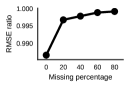
(a) Balding-Nichols

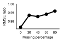
(b) TGP

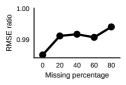
(c) HDGP

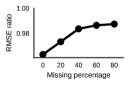
(d) PSD $(\alpha=0.01)$

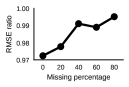
(e) Spatial $(\tau=0.1)$

Figure 4: The rmse ratio between the deconfounder with def and “No control” across simulations when only a subset of causes are unobserved. (Lower ratios means more correction.) As the percentage of observed causes decreases, the single strong ignorability is compromised; the deconfounder can no longer correct for all latent confounders.

Partially observed causes.  Finally, we study the situation where some assigned causes are unobserved, that is, where some of the SNPs are not measured. Recall that the deconfounder assumes single strong ignorability, that all single-cause confounders are observed. This assumption may be plausible when we measure all assigned causes but it may well be compromised when we only observe a subset—if a confounder affects multiple causes but only one of those causes is observed then the confounder becomes a single-cause confounder.

Using the simulated GWAS data, we randomly mask a percentage of the causes. We then use the deconfounder to estimate the causal effects of the remaining causes. To simplify the presentation, we focus on the DEF factor model. Figure 4 shows the ratio of the rmse between the deconfounder and “no control”; a ratio closer to one indicates a more biased causal estimate. Across simulations, the rmse ratio increases toward one as the percentage of observed causes decreases. With fewer observed causes, it becomes more likely for single-strong ignorability to be compromised.

Summary.  These studies provide three take-away messages: (1) The deconfounder can produce closer-to-truth causal estimates, especially when we observe many assigned causes; (2) Predictive checks reveal downstream issues with causal inference, and better factor models give better causal estimates; (3) defs can be a handy class of factor models in the deconfounder.

3.3 Case study: How do actors boost movie earnings?

We now return to the example from Section 1: How much does an actor boost (or hurt) a movie’s revenue? We study the deconfounder with the TMDB 5000 Movie Dataset. It contains 901 actors (who appeared in at least five movies) and the revenue for the 2,828 movies they appeared in. The movies span 18 genres and 58 languages. (More than 60% of the movies are in English.) We focus on the cast and the log of the revenue. Note that this is a real-world observational data set. We no longer have ground truth of causal estimates.

The idea here is that actors are potential causes of movie earnings: some actors result in greater revenue. But confounders abound. Consider the genre of a movie; it will affect both who is in the cast and its revenue. For example, an action movie tends to cast action actors, and action movies tend to earn more than family movies. And genre is just one possible confounder: movies in a series, directors, writers, language, and release season are all possible confounders.

We are interested in estimating the causal effects of individual actors on the revenue. The data are tuples of $(\mathbf{\boldsymbol{a}}_{i},y_{i})$, where $a_{ij}\in\{0,1\}$ is an indicator of whether actor $j$ in movie $i$, and $y_{i}$ is the revenue. Table 1 shows a snippet of the highest-earning movies in this dataset. The goal is to estimate the distribution of $Y_{i}(\mathbf{\boldsymbol{a}})$, the (potential) revenue as a function of a movie cast.

Deconfounded causal inference.  We apply the deconfounder. We explore four assignment models: probabilistic principal component analysis (ppca), Poisson factorization (pf), Gaussian mixture models (gmms), and deep exponential familys (defs). (Each has 50 latent dimensions; the def has structure $[50,20,5]$.) We fit each model to the observed movie casts and check the models with a predictive check on held-out data; see Section 2.4.1.

The gmm fails its check, yielding a predictive score < 0.01. The other models adequately capture patterns of actors: the checks return predictive scores of 0.12 (ppca), 0.14 (pf), and 0.15 (def). These numbers give a green light to estimate how each actor affects movie earnings.

With a fitted and checked assignment model, we estimate the causal effects of individual actors with a log-normal regression, conditional on the observed casts and “reconstructed casts,” Equation 19.

Results: Predicting the revenue of uncommon movies.  We consider test sets of uncommon movies, where we simulate an “intervention” on the types of movies that are made. This changes the distribution of casts to be different from those in the training set.

For such data, a good causal model will provide better predictions than a purely predictive model. The reason is that predictions from a causal model will work equally well under interventions as for observational data. In contrast, a non-causal model can produce incorrect predictions if we intervene on the causes (peters2016causal). This idea of invariance has also been discussed in haavelmo1944probability; aldrich1989autonomy; lanes1988logic; Pearl:2009a; scholkopf2012causal; dawid2010identifying under the terms “autonomy,” “modularity,” and “stability.”

In one test set, we hold out 10% of non-English-language movies. (Most of the movies are in English.) Table 17 compares different models in terms of the average predictive log likelihood. The deconfounder predicts better than both the purely predictive approach (no control) and a classical approach, where we condition on the observed (pre-treatment) covariates.

In another test set, we hold out 10% of movies from uncommon genres, i.e., those that are not comedies, action, or dramas. Table 18 shows similar patterns of performance. The deconfounder predicts better than purely predictive models and than those that control for available confounders.

For comparison, we finally analyze a typical test set, one drawn randomly from the data. Here we expect a purely predictive method to perform well; this is the type of prediction it is designed for. Table 16 shows the average predictive log likelihood of the deconfounder and the purely predictive method. The deconfounder predicts slightly worse than the purely predictive method.

Exploratory analysis of actors and movies.  We show how to use the deconfounder to explore the data, understanding the causal value of actors and movies.

First we examine how the coefficients of individual actors differ between a non-causal model and a deconfounded model. (In this section, we study the deconfounder with pf as the assignment model.) We explore actors with $n_{j}\beta_{j}$, their estimated coefficients scaled by the number of movies they appeared in. This quantity represents how much of the total log revenue is “explained” by actor $j$.

Consider the top 25 actors in both the corrected and uncorrected models. In the uncorrected model, the top actors are movie stars such as Tom Cruise, Tom Hanks, and Will Smith. Some actors, like Arnold Schwartzenegger, Robert De Niro, and Brad Pitt, appear in the top-25 uncorrected coefficients but not in the top-25 corrected coefficients. In their place, the top 25 causal actors include actors that do not appear in as many blockbusters, such as Owen Wilson, Nick Cage, Cate Blanchett, and Antonio Banderes.

Also consider the actors whose estimated contribution improves the most from the non-causal to the causal model. The top five “most improved” actors are Stanley Tucci, Willem Dafoe, Susan Sarandon, Ben Affleck, and Christopher Walken. These (excellent) actors often appear in smaller movies.

Next we look at how the deconfounder changes the causal estimates of movie casts. We can calculate the movie casts whose causal estimates are decreased most by the deconfounder. The “causal estimate of a cast” is the predicted revenue without including the term that involves the confounder; this is the portion of the predicted log revenue that is attributed to the cast.

At the top of this list are blockbuster series. Among the top 25 include all of the X-Men movies, all of the Avengers movies, and all of the Ocean’s X movies. Though unmeasured in the data, being part of a series is a confounder. It affects both the casting and the revenue of the movie: sequels must contain recurring characters and they are only made when the producers expect to profit. In capturing the correlations among casts, the deconfounder corrects for this phenomenon.

4 Theory

We develop theoretical results around the deconfounder. (All proofs and proof sketches are in the appendix.)

We first justify the use of factor models by connecting them to the ignorability assumption. We show that factor models imply ignorability. We next establish theoretical properties of the substitute confounder: it captures all multi-cause confounders and it does not capture any mediators. These results imply that if the factor model captures the distribution of the assigned causes then the substitute confounder renders the assignment ignorable. Moreover, such a factor model always exists.

We then discuss a collection of identification results around the deconfounder. Under stable unit treatment value assumption (sutva) and single ignorability, we prove that the deconfounder identifies the average causal effects and the conditional potential outcomes under different conditions.

4.1 Factor models and the substitute confounder

To study the deconfounder, we first connect ignorability to factor models. Recall the definitions of ignorability and factor model.

Ignorability assumes that the assigned causes are conditionally independent of the potential outcomes (rosenbaum1983central):

Definition 1.

(Ignorability) Assigned causes are ignorable given $Z_{i}$ if

$$(A_{i1},\ldots,A_{im})\mathchoice{\mathrel{\hbox to0.0pt{$\displaystyle\perp$\hss}\mkern 2.0mu{\displaystyle\perp}}}{\mathrel{\hbox to0.0pt{$\textstyle\perp$\hss}\mkern 2.0mu{\textstyle\perp}}}{\mathrel{\hbox to0.0pt{$\scriptstyle\perp$\hss}\mkern 2.0mu{\scriptstyle\perp}}}{\mathrel{\hbox to0.0pt{$\scriptscriptstyle\perp$\hss}\mkern 2.0mu{\scriptscriptstyle\perp}}}Y_{i}(\mathbf{\boldsymbol{a}})\,|\,Z_{i}$$ (35)

for all $(a_{1},\ldots,a_{m})\in\mathcal{A}_{1}\otimes\cdots\otimes\mathcal{A}_{m},$, and $i=1,\ldots,n$.

Roughly, the assigned causes are ignorable given $Z_{i}$ if all confounders are captured by $Z_{i}$. More precisely, the assigned causes are ignorable if all confounders are measurable with respect to the $\sigma$-algebra generated by $Z_{i}$.

A factor model of assigned causes describes each assigned cause of a individual with a latent variable specific to this individual and another specific to this cause:

Definition 2.

(Factor model of assigned causes) Consider the assigned causes $\mathbf{\boldsymbol{A}}_{1:n}$, a set of latent variables $Z_{1:n}$ and a set of parameters $\theta_{1:m}$. A factor model of the assigned causes is a latent-variable model,

$$p(z_{1:n},\mathbf{\boldsymbol{a}}_{1:n}\,;\,\theta_{1:m})=p(z_{1:n})\prod_{i=1}^{n}\prod_{j=1}^{m}p(a_{ij}\,|\,z_{i},\theta_{j}).$$ (36)

The distribution of assigned causes is the corresponding marginal,

$$p(\mathbf{\boldsymbol{a}}_{1:n})=\int p(z_{1:n},\mathbf{\boldsymbol{a}}_{1:n}\,;\,\theta_{1:m})\mathop{}\!\mathrm{d}z_{1:n}.$$ (37)

In a factor model, each latent variable $Z_{i}$ of individual $i$ renders its assigned causes $A_{ij},j=1,\ldots,m,$ conditionally independent. Each cause is accompanied with an unknown parameter $\theta_{j}$. As we mentioned in Section 2.4.1, many common models from Bayesian statistics and machine learning can be written as factor models.

To connect ignorability to factor models, consider an intermediate construct, the “Kallenberg construction.” The Kallenberg construction is inspired by the idea of randomization variables, Uniform[0,1] variables from which we can construct a random variable with an arbitrary distribution (kallenbergfoundations). The Kallenberg construction of assigned causes will bridge the conditional independence statement in Equation 35 with the factor models of the deconfounder.

Definition 3.

(Kallenberg construction of assigned causes) Consider a random variable $Z_{i}$ taking values in $\mathcal{Z}$. The distribution of assigned causes $(A_{i1},\ldots,A_{im})$ admits a Kallenberg construction if there exists (deterministic) measurable functions, $f_{j}:\mathcal{Z}\times[0,1]\rightarrow\mathcal{A}_{j}$ and random variables $U_{ij}\in[0,1]$ ($j=1,\ldots,m$) such that

$$A_{ij}\stackrel{{\scriptstyle a.s.}}{{=}}f_{j}(Z_{i},U_{ij}).$$ (38)

The variables $U_{ij}$ must marginally follow Uniform[0,1] and jointly satisfy

$$(U_{i1},\ldots,U_{im})\mathchoice{\mathrel{\hbox to0.0pt{$\displaystyle\perp$\hss}\mkern 2.0mu{\displaystyle\perp}}}{\mathrel{\hbox to0.0pt{$\textstyle\perp$\hss}\mkern 2.0mu{\textstyle\perp}}}{\mathrel{\hbox to0.0pt{$\scriptstyle\perp$\hss}\mkern 2.0mu{\scriptstyle\perp}}}{\mathrel{\hbox to0.0pt{$\scriptscriptstyle\perp$\hss}\mkern 2.0mu{\scriptscriptstyle\perp}}}(Z_{i},Y_{i}(a_{1},\ldots,a_{m}))$$ (39)

for all $(a_{1},\ldots,a_{m})\in\mathcal{A}_{1}\otimes\cdots\otimes\mathcal{A}_{m}$.

Using these definitions, the first lemma relates ignorability to the Kallenberg construction.

Lemma 1.

(Kallenberg construction $\Leftrightarrow$ strong ignorability) The assigned causes are ignorable given a random variable $Z_{i}$ if and only if the distribution of the assigned causes $(A_{i1},\ldots,A_{im})$ admits a Kallenberg construction from $Z_{i}$.

What Lemma 1 says is that if the distribution of the assigned causes has a Kallenberg construction from a random variable $Z_{i}$ then $Z_{i}$ is a valid substitute confounder: it renders the causes ignorable. Moreover, a valid substitute confounder must always come from a Kallenberg construction.

We next relate the Kallenberg construction to factor models. We show that factor models admit a Kallenberg construction. This fact suggests the deconfounder: if we fit a factor model to capture the distribution of assigned causes then we can use the fitted factor model to construct a substitute confounder.

Lemma 2.

(factor models $\Rightarrow$ Kallenberg construction) Under weak regularity conditions and single ignorability, every factor model of the assigned causes $p(\theta_{1:m},z_{1:n},\mathbf{\boldsymbol{a}}_{1:n})$ admits a Kallenberg construction from $Z_{i}$.

Lemma 1 and Lemma 2 connect ignorability to Kallenberg constructions and then Kallenberg constructions to factor models. The two lemmas together connect factor models to ignorability. These connections enable the deconfounder: they explain how the distribution of assigned causes relates to the substitute confounder $Z$ in a Kallenberg construction. They justify why we can take a set of assigned causes and do inference on $Z$ via factor models.

Next we establish two properties of the substitute confounder. We assume the substitute confounder comes from a factor model that captures the population distribution of the causes.

The first property is that the substitute confounder must capture all multi-cause confounders. It implies that the inferred substitute confounder, together with all single-cause confounders (if there is any), deconfounds causal inference.

Lemma 3.

Any multi-cause confounder $C_{i}$ must be measurable with respect to the $\sigma$-algebra generated by the substitute confounder $Z_{i}$.

A multi-cause confounder is a confounder that confounds two or more causes. (Its technical definition stems from Definition 4 of vanderweele2013definition; see Appendix E.) Figure 1 gives the intuition with a graphical model and Appendix E gives a detailed proof.

Lemma 3 shows that the deconfounder captures unobserved confounders. But might the inferred substitute confounder pick up a mediator? If the substitute confounder also picks up a mediator then conditioning on it will yield conservative causal estimates (baron1986moderator; imai2010identification). The next proposition alleviates this concern.

Lemma 4.

Any mediator is almost surely not measurable with respect to the $\sigma$-algebra generated by the substitute confounder $Z_{i}$ and the pre-treatment observed covariates $X_{i}$.

Lemma 4 implies that the substitute confounder does not pick up mediators, variables along the path between causes and effects. This property greenlights us for treating the inferred substitute confounder as a pre-treatment covariate.

Lemma 3 and Lemma 4 qualify the substitute confounder for mimicking confounders. We condition on the substitute confounder and proceed with causal inference.

These lemmas lead to justifications of the deconfounder algorithm. We first describe their implications on the substitute confounders and factor models.

Proposition 5.

(Substitute confounders and factor models) Under weak regularity conditions,

1. Under single ignorability, the assigned causes are ignorable given the substitute confounder $Z_{i}$ and the pre-treatment covariates $X_{i}$ if the true distribution $p(\mathbf{\boldsymbol{a}}_{1:n})$ can be written as a factor model that uses the substitute confounder, $p(z_{1:n},\mathbf{\boldsymbol{a}}_{1:n}\,|\,\theta_{1:m})$.

2. There always exists a factor model that captures the distribution of assigned causes.

Proof sketch.

The first part follows from Lemmas 1 and 2. The second part follows from the Reichenbach’s common cause principle (Peters2017; sober1976simplicity) and Sklar’s theorem (sklar1959fonctions): any multivariate joint distribution can be factorized into the product of univariate marginal distributions and a copula which describes the dependence structure between the variables. The full proof is in Appendix D. ∎

Proposition 5 justifies the use of factor models in the deconfounder. The first part of Proposition 5 suggests how to find a valid substitute confounder, one that renders the causes strongly ignorable. Two conditions suffice: (1) the substitute confounder comes from a factor model; (2) the factor model captures the population distribution of the assigned causes. The assignment model in the deconfounder stems from this result: fit a factor model to the assigned causes, check that it captures their population distribution, and finally use the fitted factor model to infer a substitute confounder. The first part of the theorem says that the deconfounder does deconfound. The second part ensures that there is hope to find a deconfounding factor model. There always exists a factor model that captures the population distribution of the assigned causes.

4.2 Causal identification of the deconfounder

Building on the characterizations of the substitute confounder (Lemmas 2, 1, 3 and 4), we discuss a collection of causal identification results around the deconfounder. We prove that the deconfounder can identify three causal quantities under suitable conditions. These causal quantities include the average causal effect of all the causes, the average causal effect of subsets of the causes, and the conditional potential outcome.

Before stating the identification results, we first describe the notion of a consistent substitute confounder; we will rely on this notion for identification.

Definition 4.

(Consistency of substitute confounders) The factor model $p(\theta,z,\mathbf{\boldsymbol{a}})$ admits consistent estimates of the substitute confounder $Z_{i}$ if, for some function $f_{\theta}$,

$$p(z_{i}\,|\,\mathbf{\boldsymbol{a}}_{i},\theta)=\delta_{f_{\theta}(\mathbf{\boldsymbol{a}}_{i})}.$$ (40)

Consistency of substitute confounders requires that we can estimate the substitute confounder $Z_{i}$ from the causes $\mathbf{\boldsymbol{A}}_{i}$ with certainty; it is a deterministic function of the causes. Nevertheless, the substitute confounder need not coincide with the true data-generating $Z_{i}$; nor does it need to coincide with the true unobserved confounder. We only need to estimate the substitute confounder $Z_{i}$ up to some deterministic bijective transformations (e.g. scaling and linear transformations).

Many factor models admit consistent substitute confounder estimates when the number of causes is large. For example, probabilistic PCA and Poisson factorization lead to consistent $Z_{i}$ as $(n+m)\cdot\log(nm)/(nm)\rightarrow 0$, where $n$ is the number of individuals and $m$ is the number of causes (chen2017structured). Many studies also involve many causes, e.g. the genome-wide association studies (gwas) study in Section 3.2 and the movie-actor study in Section 3.3.

We now describe three identification results under sutva, single ignorability, and consistency of substitute confounders. We first study the average causal effect of all the causes.

Theorem 6.

(Identification of the average causal effect of all the causes) Assume sutva, single ignorability, and consistency of substitute confounders. Then, under conditions described below, the deconfounder non-parametrically identifies the average causal effect of all the causes. The average causal effect of changing the causes from $\mathbf{\boldsymbol{a}}=(a_{1},\ldots,a_{m})$ to $\mathbf{\boldsymbol{a}}^{\prime}=(a^{\prime}_{1},\ldots,a^{\prime}_{m})$ is

$$\mathbb{E}_{Y}\left[Y_{i}(\mathbf{\boldsymbol{a}})\right] -\mathbb{E}_{Y}\left[Y_{i}(\mathbf{\boldsymbol{a}}^{\prime})\right]=\mathbb{E}_{Z,X}\left[\mathbb{E}_{Y}\left[Y_{i}\,|\,\mathbf{\boldsymbol{A}}_{i}=\mathbf{\boldsymbol{a}},Z_{i},X_{i}\right]\right]-\mathbb{E}_{Z,X}\left[\mathbb{E}_{Y}\left[Y_{i}\,|\,\mathbf{\boldsymbol{A}}_{i}=\mathbf{\boldsymbol{a}}^{\prime},Z_{i},X_{i}\right]\right].$$ (41)

This holds with the following two conditions: (1) The substitute confounder is a piece-wise constant function of the (continuous) causes: $\nabla_{\mathbf{\boldsymbol{a}}}f_{\theta}(\mathbf{\boldsymbol{a}})=0$ up to a set of Lebesgue measure zero; (2) The outcome is separable,

$$\mathbb{E}\left[Y_{i}(\mathbf{\boldsymbol{a}})\,|\,Z_{i}=z,X_{i}=x\right] =f_{1}(\mathbf{\boldsymbol{a}},x)+f_{2}(z),$$

$$\mathbb{E}\left[Y_{i}\,|\,\mathbf{\boldsymbol{A}}_{i}=\mathbf{\boldsymbol{a}},Z_{i}=z,X_{i}=x\right] =f_{3}(\mathbf{\boldsymbol{a}},x)+f_{4}(z),$$

for all $(\mathbf{\boldsymbol{a}},x,z)\in\mathcal{A}\times\mathcal{X}\times\mathcal{Z}$ and some continuously differentiable functions $f_{1}$, $f_{2}$, $f_{3}$, and $f_{4}$.

Proof sketch.

Theorem 6 rely on two results: (1) Single ignorability and Lemma 3 ensure $(Z_{i},X_{i})$ capture all confounders; (2) The pre-treatment nature of $X_{i}$ and Lemma 4 ensure $(Z_{i},X_{i})$ capture no mediators. These results assert ignorability given the substitute confounder $Z_{i}$ and the observed covariates $X_{i}$. They greenlight us for causal inference given consistency of substitute confounder estimates. Theorem 6 then leverages two additional conditions to identify average causal effects without assuming overlap. The full proof is in Appendix H. ∎

Theorem 6 shows that the deconfounder can unbiasedly estimate the average causal effect of all the causes. It requires two conditions beyond single ignorability, sutva, and consistency of substitute confounders. The first condition requires that the substitute confounder be a piece-wise constant function; it is satisfied when the substitute confounder is discrete and the causes are continuous. The second condition requires that the potential outcome be separable in the substitute confounder and the causes; the observed data also respects this separability. This condition is satisfied when the substitute confounder does not interact with the causes. For example, this condition is often satisfied in gwas studies: the effect of snp s on a trait does not depend on an individual’s ancestry.

When the separability condition of Theorem 6 does not hold, we can still use the deconfounder to handle the unobserved multi-cause confounders that do not interact with the causes. As long as the observed covariates include those that do interact with the causes, the deconfounder produces unbiased estimates of the average causal effect.

We next discuss the identification of the average causal effect for subsets of the causes.

Theorem 7.

(Identification of the average causal effect of subsets of the causes) Assume sutva, single ignorability, and consistency of substitute confounders. Then, under the condition described below, the deconfounder non-parametrically identifies the average causal effect of subsets of causes. The average causal effect of changing the first $k\leavevmode\nobreak\ (k<m)$ causes from $a_{1:k}=(a_{1},\ldots,a_{k})$ to $a^{\prime}_{1:k}=(a^{\prime}_{1},\ldots,a^{\prime}_{k})$ is

$$\mathbb{E}_{A_{(k+1):m}}\left[\mathbb{E}_{Y}\left[Y_{i}(a_{1:k},A_{i,(k+1):m})\right]\right]-\mathbb{E}_{A_{(k+1):m}}\left[\mathbb{E}_{Y}\left[Y_{i}(a^{\prime}_{1:k},A_{i,(k+1):m})\right]\right]$$

$$= \mathbb{E}_{Z,X}\left[\mathbb{E}_{Y}\left[Y_{i}\,|\,Z_{i},X_{i},A_{i,1:k}=a_{1:k}\right]\right]-\mathbb{E}_{Z,X}\left[\mathbb{E}_{Y}\left[Y_{i}\,|\,Z_{i},X_{i},A_{i,1:k}=a^{\prime}_{1:k}\right]\right].$$

This holds with the following condition: The first $k$ causes $A_{i1},\ldots,A_{ik}$ satisfy overlap, $P((A_{i1},\ldots,A_{ik})\in\mathcal{A}\,|\,Z_{i},X_{i})>0$ for any set $\mathcal{A}$ such that $P(\mathcal{A})>0$.

Proof sketch.

Similar to Theorem 6, Theorem 7 uses Lemma 3 and Lemma 4 to greenlight the use of a substitute confounder. It then relies on overlap to identify the average causal effect; we follow the classical argument that identifies the average treatment effect (Imbens:2015). The full proof is in Appendix I. ∎

Theorem 7 shows that the deconfounder can unbiasedly estimate the average causal effect of subsets of the causes. It lets us answer “how would the movie revenue change, on average, if we place Meryl Streep and Sean Connery into a movie?” Beyond single ignorability, sutva, and consistency of substitute confounders, Theorem 7 requires overlap. Overlap ensures that $\mathbb{E}_{Y}\left[Y_{i}\,|\,Z_{i},X_{i},A_{i,1:k}=a_{1:k}\right]$ is estimable from the observed data for all possible values of $(Z_{i},X_{i},A_{i,1:k})$. The overlap assumption about the causes in Theorem 7 replaces the separability assumption about the outcome model required by Theorem 6.

We note that the overlap condition and the consistency of substitute confounders are compatible. Though consistency requires $P(Z_{i}\,|\,\mathbf{\boldsymbol{A}}_{i})=\delta_{f_{\theta}(\mathbf{\boldsymbol{A}}_{i})}$, it is still possible for subsets of the causes to satisfy overlap; the consistency condition only prevents the complete set of $m$ causes from satisfying overlap. For example, consider a consistent estimate of the substitute confounder that is one-dimensional, $Z_{i}=\sum_{j=1}^{m}\alpha_{j}A_{ij}$. Any $k\leq m-1$ causes satisfy overlap, but the complete set of $m$ causes do not.

Finally, we discuss the identification of the conditional mean potential outcome.

Theorem 8.

(Identification of the conditional mean potential outcome) Assume sutva, single ignorability, and consistency of substitute confounders. Then, under the condition described below, the deconfounder non-parametrically identifies the mean potential outcome of an individual given its current assigned causes. If an individual is assigned with $\mathbf{\boldsymbol{a}}=(a_{1},\ldots,a_{m})$, then its potential outcome under a different assignment $\mathbf{\boldsymbol{a}}^{\prime}=(a^{\prime}_{1},\ldots,a^{\prime}_{m})$ is

$$\mathbb{E}_{Y}\left[Y_{i}(\mathbf{\boldsymbol{a}}^{\prime})\,|\,\mathbf{\boldsymbol{A}}_{i}=\mathbf{\boldsymbol{a}}\right]=\mathbb{E}_{Z,X}\left[\mathbb{E}_{Y}\left[Y_{i}\,|\,Z_{i},X_{i},\mathbf{\boldsymbol{A}}_{i}=\mathbf{\boldsymbol{a}}\right]\right].$$

This holds with the following condition: The cause assignment of interest $\mathbf{\boldsymbol{a}}^{\prime}$ leads to the same substitute confounder estimate as the observed assigned causes: $P(Z_{i}\,|\,\mathbf{\boldsymbol{A}}_{i}=\mathbf{\boldsymbol{a}})=P(Z_{i}\,|\,\mathbf{\boldsymbol{A}}_{i}=\mathbf{\boldsymbol{a}}^{\prime})$.

Proof sketch.

As with Theorem 6 and Theorem 7, Theorem 8 relies on the ignorability given the substitute confounders $Z_{i}$ and the observed covariates $X_{i}$ due to Lemma 3 and Lemma 4. It then identifies the potential outcome by focusing on the data points with the same substitute confounder estimate. We note that this identification result does not require overlap. The full proof is in Appendix J. ∎

Given consistency of substitute confounders, Theorem 8 nonparametrically identifies the mean potential outcome of an individual $Y_{i}(\mathbf{\boldsymbol{a}}^{\prime})$ given its current assigned causes $\mathbf{\boldsymbol{A}}_{i}=\mathbf{\boldsymbol{a}}$. The only requirement is about the configurations of cause assignments we can query, $\mathbf{\boldsymbol{a}}^{\prime}$; these configurations should lead to the same substitute confounder estimate as the current assigned causes.

We illustrate this condition with actors causing movie revenue. For simplicity, assume the substitute confounder captures the genre of each movie. Start with one of the James Bond movie; it is a spy film. We can ask what its revenue would be if we make its cast to be that of “The Bourne Trilogy” (also a spy film). Alternatively, we can query what if we make its cast to include some actors from “The Bourne Trilogy” and other actors from “North By Northwest”; both are spy films. However, we can not query what if we make its cast to be that of “The Shawshank Redemption” (which is not a spy film).

Theorems 6, 7 and 8 confirm the validity of the deconfounder by providing three sets of nonparametric identification results. When the assumptions in Theorems 6, 7 and 8 do not hold, we recommend evaluating the uncertainty of the deconfounder estimate. Section 2.6.8 discusses how; Section 3.1 gives an example. The posterior distribution of the deconfounder estimate reflects how the (finite) observed data informs causal quantities of interest. When the causal quantity is non-identifiable, the posterior distribution of the deconfounder estimate will reflect this non-identifiability. For example, if the causal quantity is non-identifiable over $\mathcal{R}$, the posterior distribution of the deconfounder estimate will be uniform over $\mathcal{R}$ (with non-informative priors).

We finally remark that the identification results in Theorems 6, 7 and 8 do not contradict the negative results of d2019multi. d2019multi explore nonparametric non-identification of a particular causal quantity, the mean potential outcome $\mathbb{E}\left[Y_{i}(\mathbf{\boldsymbol{a}})\right]$. In this paper, Theorems 6, 7 and 8 establish the nonparametric identification of different causal quantities. d2019multi do not make the same assumptions as in Theorems 6, 7 and 8. More specifically, under consistency of substitute confounders and other suitable conditions, Theorem 6 shows that the average causal effect of all the causes $\mathbb{E}\left[Y_{i}(\mathbf{\boldsymbol{a}})\right]-\mathbb{E}\left[Y_{i}(\mathbf{\boldsymbol{a}}^{\prime})\right]$ is nonparametrically identifiable; Theorem 7 shows that the average causal effect of subsets of the causes $\mathbb{E}_{A_{(k+1):m}}\left[\mathbb{E}_{Y}\left[Y_{i}(a_{1:k},A_{i,(k+1):m})\right]\right]-\mathbb{E}_{A_{(k+1):m}}\left[\mathbb{E}_{Y}\left[Y_{i}(a^{\prime}_{1:k},A_{i,(k+1):m})\right]\right]$ is nonparametrically identifiable; Theorem 8 shows that the conditional mean potential outcome $\mathbb{E}\left[Y_{i}(\mathbf{\boldsymbol{a}}^{\prime})\,|\,\mathbf{\boldsymbol{A}}_{i}=\mathbf{\boldsymbol{a}}\right]$ is nonparametrically identifiable.

5 Discussion

Classical causal inference studies how a univariate cause affects an outcome. Here we studied multiple causal inference, where there are multiple causes that contribute to the effect. Multiple causes might at first appear to be a curse, but we showed that it can be a blessing. Multiple causal inference liberates us from ignorability, providing causal inference from observational data under weaker assumptions than the classical approach requires.

We developed the deconfounder: first fit a good factor model of assigned causes; then use the factor model to infer a substitute confounder; finally perform causal inference. We showed how a substitute confounder from a good factor model must capture all multi-cause confounders, and we demonstrated that whether a factor model is satisfactory is a checkable proposition.

There are many directions for future work.

Here we estimate the potential outcomes under all configurations of the causes. Which of these potential outcomes can be reliably estimated? Can we optimally trade off confounding bias and estimation variance?

Here we checked factor models for downstream causal unbiasedness. But model checking is still an imprecise science. Can we develop rigorous model checking algorithms for causal inference?

Here we focused on estimation. Can we develop a testing counterpart? How can we identify significant causes while still preserving family-wise error rate or false discovery rate?

Here we analyzed univariate outcomes. Can we work with both multiple causes and multiple outcomes. Can dependence among outcomes further help causal inference?

Acknowledgments.   We have had many useful discussions about the previous versions of this manuscript. We thank Edo Airoldi, Elias Barenboim, Léon Bottou, Alexander D’Amour, Barbara Engelhart, Andrew Gelman, David Heckerman, Jennifer Hill, Ferenc Huszár, George Hripcsak, Daniel Hsu, Guido Imbens, Thorsten Joachims, Fan Li, Lydia Liu, Jackson Loper, David Madigan, Suresh Naidu, Xinkun Nie, Elizabeth Ogburn, Georgia Papadogeorgou, Judea Pearl, Alex Peysakhovich, Rajesh Ranganath, Jason Roy, Cosma Shalizi, Dylan Small, Hal Stern, Amos Storkey, Wesley Tansey, Eric Tchetgen Tchetgen, Dustin Tran, Victor Veitch, Stefan Wager, Kilian Weinberger, Jeannette Wing, Linying Zhang, Qingyuan Zhao, and José Zubizarreta.

Appendix

Appendix A Detailed Results of the GWAS Study

In this section, we present tables of results from the gwas study in Section 3.2.

Appendices A, A, A, A and A contain the result under the high snr setting.

		Real-valued outcome	Binary outcome
	Pred. check	rmse $\times 10^{-2}$	rmse $\times 10^{-2}$
No control	—	49.66	39.39
Control for confounders∗	—	40.27	31.09
1-4 (G)LMM	—	46.22	37.81
PPCA	0.13	46.05	36.01
PF	0.15	44.58	36.30
LFA	0.14	43.02	36.65
GMM	0.01	47.33	40.24
DEF	0.18	41.05	33.88

Table 6: GWAS high-snr simulation I: Balding-Nichols Model. (“Control for all confounders” means including the unobserved confounders as covariates.) The deconfounder outperforms (G)LMM; DEF performs the best among the five factor models. Predictive checking offers a good indication of when the deconfounder fails.

		Real-valued outcome	Binary outcome
	Pred. check	rmse $\times 10^{-2}$	rmse $\times 10^{-2}$
No control	—	68.78	38.16
Control for confounders∗	—	60.29	32.76
1-4 (G)LMM	—	65.25	35.41
PPCA	0.15	65.98	36.11
PF	0.17	64.25	34.79
LFA	0.17	64.00	37.08
GMM	0.02	67.23	35.40
DEF	0.20	63.73	33.71

Table 7: GWAS high-snr simulation II: 1000 Genomes Project (TGP). (“Control for all confounders” means including the unobserved confounders as covariates.) The deconfounder outperforms (G)LMM; DEF performs the best among the five factor models. Predictive checking offers a good indication of when the deconfounder fails.

		Real-valued outcome	Binary outcome
	Pred. check	rmse $\times 10^{-2}$	rmse $\times 10^{-2}$
No control	—	77.35	45.93
Control for confounders∗	—	67.53	39.43
1-4 (G)LMM	—	74.38	42.79
PPCA	0.14	74.45	43.27
PF	0.14	71.40	42.75
LFA	0.13	72.11	42.34
GMM	0.03	76.27	46.88
DEF	0.16	69.86	41.61

Table 8: GWAS high-snr simulation III: Human Genome Diversity Project (HGDP). (“Control for confounders” means including the unobserved confounders as covariates.) The deconfounder outperforms (G)LMM; DEF performs the best among the five factor models. Predictive checking offers a good indication of when the deconfounder fails.

			Real-valued outcome	Binary outcome
		Pred. check	rmse $\times 10^{-2}$	rmse $\times 10^{-2}$
$\alpha=0.01$	No control	—	40.68	30.37
	Control for confounders∗	—	34.35	28.21
1-5	(G)LMM	—	39.09	28.36
	PPCA	0.15	38.14	28.97
	PF	0.16	34.77	28.67
	LFA	0.16	35.87	28.33
	GMM	0.02	38.15	29.69
	DEF	0.18	34.84	28.04
$\alpha=0.1$	No control	—	43.87	36.77
	Control for confounders∗	—	37.62	33.89
1-5	(G)LMM	—	39.97	35.76
	PPCA	0.21	39.60	35.61
	PF	0.19	38.95	34.28
	LFA	0.18	39.28	34.73
	GMM	0.00	44.38	36.44
	DEF	0.20	38.75	34.85
$\alpha=0.5$	No control	—	47.38	41.84
	Control for confounders∗	—	43.63	39.86
1-5	(G)LMM	—	47.28	42.91
	PPCA	0.14	46.90	41.41
	PF	0.16	43.29	40.69
	LFA	0.17	43.60	40.77
	GMM	0.02	46.95	42.47
	DEF	0.18	43.09	40.03
$\alpha=1.0$	No control	—	53.94	49.32
	Control for confounders∗	—	47.12	45.96
1-5	(G)LMM	—	49.21	48.96
	PPCA	0.21	50.57	47.58
	PF	0.19	48.07	46.16
	LFA	0.17	49.27	46.16
	GMM	0.02	52.28	50.31
	DEF	0.23	47.82	45.62

Table 9: GWAS high-snr simulation IV: Pritchard-Stephens-Donnelly (PSD). (“Control for confounders” means including the unobserved confounders as covariates.) The deconfounder outperforms (G)LMM; DEF often performs the best among the five factor models. Predictive checking offers a good indication of when the deconfounder fails.

			Real-valued outcome	Binary outcome
		Pred. check	rmse $\times 10^{-2}$	rmse $\times 10^{-2}$
$\tau=0.1$	No control	—	47.47	45.16
	Control for confounders∗	—	44.22	43.85
1-5	(G)LMM	—	47.35	44.15
	PPCA	0.08	47.61	44.36
	PF	0.09	47.13	43.69
	LFA	0.09	47.16	43.87
	GMM	0.01	47.55	45.95
	DEF	0.10	46.95	43.62
$\tau=0.25$	No control	—	44.68	41.10
	Control for confounders∗	—	41.23	39.65
1-5	(G)LMM	—	43.42	40.67
	PPCA	0.11	43.26	41.28
	PF	0.12	43.30	41.10
	LFA	0.13	43.62	41.65
	GMM	0.01	44.81	41.02
	DEF	0.13	43.35	40.97
$\tau=0.5$	No control	—	45.18	40.92
	Control for confounders∗	—	41.33	37.35
1-5	(G)LMM	—	44.83	40.59
	PPCA	0.10	43.78	39.99
	PF	0.09	43.65	40.23
	LFA	0.10	43.88	40.04
	GMM	0.01	46.08	40.76
	DEF	0.12	43.57	40.02
$\tau=1.0$	No control	—	56.57	57.70
	Control for confounders∗	—	52.98	55.46
1-5	(G)LMM	—	56.44	56.33
	PPCA	0.14	55.18	57.36
	PF	0.12	55.29	56.31
	LFA	0.13	54.75	56.66
	GMM	0.01	57.15	57.55
	DEF	0.12	55.07	56.22

Table 10: GWAS high-snr simulation V: Spatial model. (“Control for confounders” means including the unobserved confounders as covariates.) The deconfounder often outperforms (G)LMM. Predictive checking offers a good indication of when the deconfounder fails: GMM poorly captures the SNPs; it can amplify the error in causal estimates.

Appendices A, A, A, A and A contain the result under the low snr setting.

		Real-valued outcome	Binary outcome
	Pred. check	rmse $\times 10^{-2}$	rmse $\times 10^{-2}$
No control	—	6.55	5.75
Control for confounders∗	—	6.54	5.75
1-4 (G)LMM	—	6.54	5.74
PPCA	0.14	6.52	5.74
PF	0.16	6.53	5.74
LFA	0.14	6.54	5.74
GMM	0.01	6.54	5.74
DEF	0.19	6.47	5.74

Table 11: GWAS low-snr simulation I: Balding-Nichols Model. (“Control for all confounders” means including the unobserved confounders as covariates.) The deconfounder outperforms LMM; DEF performs the best among the five factor models; it also outperforms using the (unobserved) confounder information. Predictive checking offers a good indication of when the deconfounder fails.

		Real-valued outcome	Binary outcome
	Pred. check	rmse $\times 10^{-2}$	rmse $\times 10^{-2}$
No control	—	8.31	4.85
Control for confounders∗	—	8.28	4.85
1-4 (G)LMM	—	8.29	4.85
PPCA	0.14	8.29	4.85
PF	0.15	8.29	4.85
LFA	0.17	8.26	4.85
GMM	0.02	8.30	4.85
DEF	0.20	8.11	4.84

Table 12: GWAS low-snr simulation II: 1000 Genomes Project (TGP). (“Control for all confounders” means including the unobserved confounders as covariates.) The deconfounder outperforms LMM; DEF performs the best among the five factor models; it also outperforms using the (unobserved) confounder information. Predictive checking offers a good indication of when the deconfounder fails.

		Real-valued outcome	Binary outcome
	Pred. check	rmse $\times 10^{-2}$	rmse $\times 10^{-2}$
No control	—	9.59	5.84
Control for confounders∗	—	9.52	5.84
1-4 (G)LMM	—	9.57	5.84
PPCA	0.14	9.55	5.84
PF	0.13	9.56	5.84
LFA	0.14	9.54	5.84
GMM	0.03	9.59	5.84
DEF	0.16	9.47	5.83

Table 13: GWAS low-snr simulation III: Human Genome Diversity Project (HGDP). (“Control for confounders” means including the unobserved confounders as covariates.) The deconfounder outperforms LMM; DEF performs the best among the five factor models; it also outperforms using the (unobserved) confounder information. Predictive checking offers a good indication of when the deconfounder fails.

			Real-valued outcome	Binary outcome
		Pred. check	rmse $\times 10^{-2}$	rmse $\times 10^{-2}$
$\alpha=0.01$	No control	—	3.73	3.23
	Control for confounders∗	—	3.71	3.23
1-5	(G)LMM	—	3.71	3.23
	PPCA	0.13	3.64	3.23
	PF	0.16	3.67	3.23
	LFA	0.16	3.66	3.23
	GMM	0.02	3.72	3.23
	DEF	0.18	3.59	3.22
$\alpha=0.1$	No control	—	4.09	3.84
	Control for confounders∗	—	4.09	3.84
1-5	(G)LMM	—	4.09	3.84
	PPCA	0.20	4.08	3.84
	PF	0.18	4.08	3.84
	LFA	0.18	4.07	3.84
	GMM	0.00	4.09	3.84
	DEF	0.20	4.05	3.83
$\alpha=0.5$	No control	—	4.82	4.14
	Control for confounders∗	—	4.81	4.14
1-5	(G)LMM	—	4.82	4.14
	PPCA	0.14	4.81	4.13
	PF	0.17	4.80	4.13
	LFA	0.16	4.81	4.14
	GMM	0.03	4.82	4.14
	DEF	0.19	4.80	4.13
$\alpha=1.0$	No control	—	5.43	4.58
	Control for confounders∗	—	5.38	4.57
1-5	(G)LMM	—	5.40	4.58
	PPCA	0.21	5.38	4.57
	PF	0.16	5.41	4.57
	LFA	0.19	5.40	4.57
	GMM	0.02	5.43	4.58
	DEF	0.24	5.37	4.57

Table 14: GWAS low-snr simulation IV: Pritchard-Stephens-Donnelly (PSD). (“Control for confounders” means including the unobserved confounders as covariates.) The deconfounder outperforms LMM; DEF performs the best among the five factor models; it also outperforms using the (unobserved) confounder information. Predictive checking offers a good indication of when the deconfounder fails.

			Real-valued outcome	Binary outcome
		Pred. check	rmse $\times 10^{-2}$	rmse $\times 10^{-2}$
$\tau=0.1$	No control	—	4.66	4.74
	Control for confounders∗	—	4.63	4.73
1-5	(G)LMM	—	4.57	4.73
	PPCA	0.09	4.62	4.74
	PF	0.08	4.58	4.74
	LFA	0.09	4.54	4.73
	GMM	0.02	4.70	4.74
	DEF	0.10	4.53	4.73
$\tau=0.25$	No control	—	4.30	3.81
	Control for confounders∗	—	3.81	3.79
1-5	(G)LMM	—	4.28	3.80
	PPCA	0.10	4.26	3.80
	PF	0.12	4.26	3.80
	LFA	0.12	4.27	3.80
	GMM	0.01	4.30	3.81
	DEF	0.13	4.25	3.80
$\tau=0.5$	No control	—	4.30	3.85
	Control for confounders∗	—	3.82	3.83
1-5	(G)LMM	—	4.28	3.83
	PPCA	0.11	4.27	3.83
	PF	0.09	4.28	3.84
	LFA	0.11	4.27	3.84
	GMM	0.01	4.29	3.84
	DEF	0.13	4.25	3.84
$\tau=1.0$	No control	—	6.71	5.52
	Control for confounders∗	—	5.43	5.51
1-5	(G)LMM	—	6.70	5.52
	PPCA	0.14	6.70	5.52
	PF	0.12	6.70	5.52
	LFA	0.12	6.69	5.52
	GMM	0.01	6.72	5.53
	DEF	0.13	6.62	5.51

Table 15: GWAS low-snr simulation V: Spatial model. (“Control for confounders” means including the unobserved confounders as covariates.) The deconfounder often outperforms LMM; DEF often performs the best among the five factor models. Yet, the deconfounder does not outperform using the (unobserved) confounder information. Spatially-induced SNPs challenge many latent variable models to capture its patterns and fully deconfound causal inference. Predictive checking offers a good indication of when the deconfounder fails: GMM poorly captures the SNPs; it can amplify the error in causal estimates.

Appendix B Detailed Results of the Movie Study

In this section, we present tables of results from the movies study in Section 3.3.

Control	Average predictive log-likelihood
No Control	-1.1
Control for $X$	-1.1
Control for $\hat{a}_{\lx@glossaries@gls@link{acronym}{PPCA}{\leavevmode\textsc{ppca}}}$	-1.2
Control for $\hat{a}_{\lx@glossaries@gls@link{acronym}{PF}{\leavevmode\textsc{pf}}}$	-1.2
Control for $\hat{a}_{\lx@glossaries@gls@link{acronym}{DEF}{\leavevmode\textsc{def}}}$	-1.2
Control for $(\hat{a}_{\lx@glossaries@gls@link{acronym}{PPCA}{\leavevmode\textsc{ppca}}},X)$	-1.3
Control for $(\hat{a}_{\lx@glossaries@gls@link{acronym}{PF}{\leavevmode\textsc{pf}}},X)$	-1.2
Control for $(\hat{a}_{\lx@glossaries@gls@link{acronym}{DEF}{\leavevmode\textsc{def}}},X)$	-1.2

Table 16: Average predictive log-likelihood on a holdout set of all movies. ($X$ represents the observed covariates.) Causal models (the deconfounder) predicts slightly worse than prediction models.

Control	Average predictive log-likelihood
No Control	-2.5
Control for $X$	-2.1
Control for $\hat{a}_{\lx@glossaries@gls@link{acronym}{PPCA}{\leavevmode\textsc{ppca}}}$	-1.6
Control for $\hat{a}_{\lx@glossaries@gls@link{acronym}{PF}{\leavevmode\textsc{pf}}}$	-1.5
Control for $\hat{a}_{\lx@glossaries@gls@link{acronym}{DEF}{\leavevmode\textsc{def}}}$	-1.5
Control for $(\hat{a}_{\lx@glossaries@gls@link{acronym}{PPCA}{\leavevmode\textsc{ppca}}},X)$	-1.7
Control for $(\hat{a}_{\lx@glossaries@gls@link{acronym}{PF}{\leavevmode\textsc{pf}}},X)$	-1.5
Control for $(\hat{a}_{\lx@glossaries@gls@link{acronym}{DEF}{\leavevmode\textsc{def}}},X)$	-1.6

Table 17: Average predictive log-likelihood on the holdout set of non-English movies. ($X$ represents the observed covariates.) On a test set of uncommon movies, causal models with the deconfounder predict better than prediction models.

Control	Average predictive log-likelihood
No Control	-2.1
Control for $X$	-1.9
Control for $\hat{a}_{\lx@glossaries@gls@link{acronym}{PPCA}{\leavevmode\textsc{ppca}}}$	-1.4
Control for $\hat{a}_{\lx@glossaries@gls@link{acronym}{PF}{\leavevmode\textsc{pf}}}$	-1.2
Control for $\hat{a}_{\lx@glossaries@gls@link{acronym}{DEF}{\leavevmode\textsc{def}}}$	-1.3
Control for $(\hat{a}_{\lx@glossaries@gls@link{acronym}{PPCA}{\leavevmode\textsc{ppca}}},X)$	-1.4
Control for $(\hat{a}_{\lx@glossaries@gls@link{acronym}{PF}{\leavevmode\textsc{pf}}},X)$	-1.3
Control for $(\hat{a}_{\lx@glossaries@gls@link{acronym}{DEF}{\leavevmode\textsc{def}}},X)$	-1.2

Table 18: Average predictive log-likelihood on the holdout set of non-drama/comedy/action movies. ($X$ represents the observed covariates.) On a test set of uncommon movies, causal models with the deconfounder predict better than prediction models.

Appendix C Proof of Lemma 1

Proof sketch.

First assume the Kallenberg construction in Equation 38. This form shows that the assigned causes $(A_{i1},\ldots,A_{im})$ are captured by functions of $Z_{i}$ and randomization variables $U_{ij}$. This fact, in turn, implies that the randomness in $(A_{i1},\ldots,A_{im})\,|\,Z_{i}$ comes from the randomization variables which are (by definition) independent of $Y_{i}(\mathbf{\boldsymbol{a}})$. Therefore $(A_{i1},\ldots,A_{im})$ is conditionally independent of $Y_{i}$ given $Z_{i}$, i.e., ignorability holds. Now assume that ignorability holds. We prove that this assumption implies a Kallenberg construction by building on the randomization variable construction of conditional distributions (kallenbergfoundations). The full proof is in Appendix C. ∎

Proof.

For notation simplicity, we suppress the $i$ subscript in this proof.

We assume $\mathcal{Z}$ is a measurable space and $\mathcal{A}_{j},j=1,\ldots,m$ are Borel spaces.

We first prove the necessity. Assume that $A_{j}=f_{j}(Z,U_{j}),j=1,\ldots,m,$ where $f_{j},j=1,\ldots,m$ are measurable and

$$(U_{1},\ldots,U_{m})\mathchoice{\mathrel{\hbox to0.0pt{$\displaystyle\perp$\hss}\mkern 2.0mu{\displaystyle\perp}}}{\mathrel{\hbox to0.0pt{$\textstyle\perp$\hss}\mkern 2.0mu{\textstyle\perp}}}{\mathrel{\hbox to0.0pt{$\scriptstyle\perp$\hss}\mkern 2.0mu{\scriptstyle\perp}}}{\mathrel{\hbox to0.0pt{$\scriptscriptstyle\perp$\hss}\mkern 2.0mu{\scriptscriptstyle\perp}}}(Z,Y(a_{1},\ldots,a_{m}))$$ (42)

for all $(a_{1},\ldots,a_{m})$. By Proposition 5.18 in kallenbergfoundations, Equation 42 implies

$$(U_{1},\ldots,U_{m})\mathchoice{\mathrel{\hbox to0.0pt{$\displaystyle\perp$\hss}\mkern 2.0mu{\displaystyle\perp}}}{\mathrel{\hbox to0.0pt{$\textstyle\perp$\hss}\mkern 2.0mu{\textstyle\perp}}}{\mathrel{\hbox to0.0pt{$\scriptstyle\perp$\hss}\mkern 2.0mu{\scriptstyle\perp}}}{\mathrel{\hbox to0.0pt{$\scriptscriptstyle\perp$\hss}\mkern 2.0mu{\scriptscriptstyle\perp}}}_{Z}Y(a_{1},\ldots,a_{m}),$$

and so

$$(Z,U_{1},\ldots,U_{m})\mathchoice{\mathrel{\hbox to0.0pt{$\displaystyle\perp$\hss}\mkern 2.0mu{\displaystyle\perp}}}{\mathrel{\hbox to0.0pt{$\textstyle\perp$\hss}\mkern 2.0mu{\textstyle\perp}}}{\mathrel{\hbox to0.0pt{$\scriptstyle\perp$\hss}\mkern 2.0mu{\scriptstyle\perp}}}{\mathrel{\hbox to0.0pt{$\scriptscriptstyle\perp$\hss}\mkern 2.0mu{\scriptscriptstyle\perp}}}_{Z}Y(a_{1},\ldots,a_{m})$$

by Corollary 5.7 in kallenbergfoundations. It implies

$$(A_{1},\ldots,A_{m})\mathchoice{\mathrel{\hbox to0.0pt{$\displaystyle\perp$\hss}\mkern 2.0mu{\displaystyle\perp}}}{\mathrel{\hbox to0.0pt{$\textstyle\perp$\hss}\mkern 2.0mu{\textstyle\perp}}}{\mathrel{\hbox to0.0pt{$\scriptstyle\perp$\hss}\mkern 2.0mu{\scriptstyle\perp}}}{\mathrel{\hbox to0.0pt{$\scriptscriptstyle\perp$\hss}\mkern 2.0mu{\scriptscriptstyle\perp}}}_{Z}Y(a_{1},\ldots,a_{m})$$

for all $(a_{1},\ldots,a_{m})\in\mathcal{A}_{1}\otimes\cdots\otimes\mathcal{A}_{m}$. The last step is because $A_{j}$’s are measurable functions of $(Z,U_{1},\ldots,U_{m})$.

Now we prove the sufficiency. Assume that $Y(a_{1},\ldots,a_{m})\mathchoice{\mathrel{\hbox to0.0pt{$\displaystyle\perp$\hss}\mkern 2.0mu{\displaystyle\perp}}}{\mathrel{\hbox to0.0pt{$\textstyle\perp$\hss}\mkern 2.0mu{\textstyle\perp}}}{\mathrel{\hbox to0.0pt{$\scriptstyle\perp$\hss}\mkern 2.0mu{\scriptstyle\perp}}}{\mathrel{\hbox to0.0pt{$\scriptscriptstyle\perp$\hss}\mkern 2.0mu{\scriptscriptstyle\perp}}}_{Z}(A_{1},\ldots,A_{m})$. Marginalizing out all but one $A_{j}$ gives

$$Y(a_{1},\ldots,a_{m})\mathchoice{\mathrel{\hbox to0.0pt{$\displaystyle\perp$\hss}\mkern 2.0mu{\displaystyle\perp}}}{\mathrel{\hbox to0.0pt{$\textstyle\perp$\hss}\mkern 2.0mu{\textstyle\perp}}}{\mathrel{\hbox to0.0pt{$\scriptstyle\perp$\hss}\mkern 2.0mu{\scriptstyle\perp}}}{\mathrel{\hbox to0.0pt{$\scriptscriptstyle\perp$\hss}\mkern 2.0mu{\scriptscriptstyle\perp}}}_{Z}A_{j},j=1,\ldots,m.$$

By Theorem 5.10 in kallenbergfoundations, there exists a measurable function $f_{j}:\mathcal{Z}\times[0,1]\rightarrow\mathcal{A}_{j}$ and a Uniform[0,1] random variable $\tilde{U}_{j}$ satisfying $\tilde{U}_{j}\mathchoice{\mathrel{\hbox to0.0pt{$\displaystyle\perp$\hss}\mkern 2.0mu{\displaystyle\perp}}}{\mathrel{\hbox to0.0pt{$\textstyle\perp$\hss}\mkern 2.0mu{\textstyle\perp}}}{\mathrel{\hbox to0.0pt{$\scriptstyle\perp$\hss}\mkern 2.0mu{\scriptstyle\perp}}}{\mathrel{\hbox to0.0pt{$\scriptscriptstyle\perp$\hss}\mkern 2.0mu{\scriptscriptstyle\perp}}}(Z,Y(a_{1},\ldots,a_{m}))$ such that the random variable $\tilde{A}_{j}=f_{j}(Z,\tilde{U}_{j})$ satisfies

$$\tilde{A}_{j}\stackrel{{\scriptstyle d}}{{=}}A_{j}\text{ and }(\tilde{A}_{j},Z)\stackrel{{\scriptstyle d}}{{=}}(A_{j},Z).$$

Moreover, we have

$$\tilde{A}_{j}\mathchoice{\mathrel{\hbox to0.0pt{$\displaystyle\perp$\hss}\mkern 2.0mu{\displaystyle\perp}}}{\mathrel{\hbox to0.0pt{$\textstyle\perp$\hss}\mkern 2.0mu{\textstyle\perp}}}{\mathrel{\hbox to0.0pt{$\scriptstyle\perp$\hss}\mkern 2.0mu{\scriptstyle\perp}}}{\mathrel{\hbox to0.0pt{$\scriptscriptstyle\perp$\hss}\mkern 2.0mu{\scriptscriptstyle\perp}}}_{Z}Y(a_{1},\ldots,a_{m})$$

with the same argument as the above necessity part.

Hence, by Proposition 5.6 in kallenbergfoundations,

$$P(\tilde{A}_{j}\in\cdot\leavevmode\nobreak\ |\leavevmode\nobreak\ Z,Y(a_{1},\ldots,a_{m}))=P(\tilde{A}_{j}\in\cdot\leavevmode\nobreak\ |\leavevmode\nobreak\ Z)=P(A_{j}\in\cdot\leavevmode\nobreak\ |\leavevmode\nobreak\ Z)=P(A_{j}\in\cdot\leavevmode\nobreak\ |\leavevmode\nobreak\ Z,Y(a_{1},\ldots,a_{m})),$$

and so

$$(\tilde{A}_{j},Z,Y(a_{1},\ldots,a_{m}))\stackrel{{\scriptstyle d}}{{=}}(A_{j},Z,Y(a_{1},\ldots,a_{m})).$$

By Theorem 5.10 in kallenbergfoundations, we may choose some random variable $U_{j}$ such that

$$U_{j}\stackrel{{\scriptstyle d}}{{=}}\tilde{U}_{j}\text{ and }(\tilde{A}_{j},Z,Y(a_{1},\ldots,a_{m}),U_{j})\stackrel{{\scriptstyle d}}{{=}}(A_{j},Z,Y(a_{1},\ldots,a_{m}),\tilde{U}_{j}).$$

In particular, we have

$$U_{j}\mathchoice{\mathrel{\hbox to0.0pt{$\displaystyle\perp$\hss}\mkern 2.0mu{\displaystyle\perp}}}{\mathrel{\hbox to0.0pt{$\textstyle\perp$\hss}\mkern 2.0mu{\textstyle\perp}}}{\mathrel{\hbox to0.0pt{$\scriptstyle\perp$\hss}\mkern 2.0mu{\scriptstyle\perp}}}{\mathrel{\hbox to0.0pt{$\scriptscriptstyle\perp$\hss}\mkern 2.0mu{\scriptscriptstyle\perp}}}(Z,Y(a_{1},\ldots,a_{m}))$$

and

$$(A_{j},f_{j}(Z,U_{j}))\stackrel{{\scriptstyle d}}{{=}}(\tilde{A}_{j},f_{j}(Z,\tilde{U}_{j}).$$

Since

$$\tilde{A}_{j}=f_{j}(Z,\tilde{U}_{j})$$

and the diagonal in $S^{2}$ is measurable, we have

$$A_{j}\stackrel{{\scriptstyle a.s.}}{{=}}f_{j}(Z,U_{j}).$$

We then show $(U_{1},\ldots,U_{m})\mathchoice{\mathrel{\hbox to0.0pt{$\displaystyle\perp$\hss}\mkern 2.0mu{\displaystyle\perp}}}{\mathrel{\hbox to0.0pt{$\textstyle\perp$\hss}\mkern 2.0mu{\textstyle\perp}}}{\mathrel{\hbox to0.0pt{$\scriptstyle\perp$\hss}\mkern 2.0mu{\scriptstyle\perp}}}{\mathrel{\hbox to0.0pt{$\scriptscriptstyle\perp$\hss}\mkern 2.0mu{\scriptscriptstyle\perp}}}(Z,Y(a_{1},\ldots,a_{m}))$. By Theorem 5.10 in kallenbergfoundations, there exists a measurable function $g_{1}:\mathcal{Y}\times\mathcal{Z}\times[0,1]\rightarrow[0,1]$ and a Uniform[0,1] random variable $\hat{U}_{1}$ satisfying $\hat{U}_{1}\mathchoice{\mathrel{\hbox to0.0pt{$\displaystyle\perp$\hss}\mkern 2.0mu{\displaystyle\perp}}}{\mathrel{\hbox to0.0pt{$\textstyle\perp$\hss}\mkern 2.0mu{\textstyle\perp}}}{\mathrel{\hbox to0.0pt{$\scriptstyle\perp$\hss}\mkern 2.0mu{\scriptstyle\perp}}}{\mathrel{\hbox to0.0pt{$\scriptscriptstyle\perp$\hss}\mkern 2.0mu{\scriptscriptstyle\perp}}}(Y(a_{1},\ldots,a_{m}),Z)$ and

$$(Y(a_{1},\ldots,a_{m}),Z,U_{1})\stackrel{{\scriptstyle d}}{{=}}(Y(a_{1},\ldots,a_{m}),Z,g_{1}(Y(a_{1},\ldots,a_{m}),Z,\hat{U}_{1})).$$

Moreover, by

$$U_{1}\mathchoice{\mathrel{\hbox to0.0pt{$\displaystyle\perp$\hss}\mkern 2.0mu{\displaystyle\perp}}}{\mathrel{\hbox to0.0pt{$\textstyle\perp$\hss}\mkern 2.0mu{\textstyle\perp}}}{\mathrel{\hbox to0.0pt{$\scriptstyle\perp$\hss}\mkern 2.0mu{\scriptstyle\perp}}}{\mathrel{\hbox to0.0pt{$\scriptscriptstyle\perp$\hss}\mkern 2.0mu{\scriptscriptstyle\perp}}}_{Z}Y(a_{1},\ldots,a_{m}),$$

we have

$$g_{1}(Y(a_{1},\ldots,a_{m}),Z,\hat{U}_{1})\mathchoice{\mathrel{\hbox to0.0pt{$\displaystyle\perp$\hss}\mkern 2.0mu{\displaystyle\perp}}}{\mathrel{\hbox to0.0pt{$\textstyle\perp$\hss}\mkern 2.0mu{\textstyle\perp}}}{\mathrel{\hbox to0.0pt{$\scriptstyle\perp$\hss}\mkern 2.0mu{\scriptstyle\perp}}}{\mathrel{\hbox to0.0pt{$\scriptscriptstyle\perp$\hss}\mkern 2.0mu{\scriptscriptstyle\perp}}}_{Z}Y(a_{1},\ldots,a_{m})$$

there exists some measurable function $g^{\prime}_{1}:\mathcal{Z}\times[0,1]\rightarrow[0,1]$ such that

$$g_{1}(Y(a_{1},\ldots,a_{m}),Z,\hat{U}_{1})=g^{\prime}_{1}(Z,\hat{U}_{1})$$

and

$$\hat{U}_{1}\mathchoice{\mathrel{\hbox to0.0pt{$\displaystyle\perp$\hss}\mkern 2.0mu{\displaystyle\perp}}}{\mathrel{\hbox to0.0pt{$\textstyle\perp$\hss}\mkern 2.0mu{\textstyle\perp}}}{\mathrel{\hbox to0.0pt{$\scriptstyle\perp$\hss}\mkern 2.0mu{\scriptstyle\perp}}}{\mathrel{\hbox to0.0pt{$\scriptscriptstyle\perp$\hss}\mkern 2.0mu{\scriptscriptstyle\perp}}}(Z,Y(a_{1},\ldots,a_{m})).$$

In other words, we have

$$(Y(a_{1},\ldots,a_{m}),Z,U_{1})\stackrel{{\scriptstyle d}}{{=}}(Y(a_{1},\ldots,a_{m}),Z,g^{\prime}_{1}(Z,\hat{U}_{1})).$$

Repeating these steps, we again have from Theorem 5.10 in kallenbergfoundations that there exists a measurable function $g_{2}:\mathcal{Y}\times\mathcal{Z}\times[0,1]^{2}\rightarrow[0,1]$ and a Uniform[0,1] random variable $\hat{U}_{2}$ satisfying

$$\leavevmode\nobreak\ (Y(a_{1},\ldots,a_{m}),Z,U_{1},U_{2})$$

$$\stackrel{{\scriptstyle d}}{{=}} \leavevmode\nobreak\ (Y(a_{1},\ldots,a_{m}),Z,g^{\prime}_{1}(Z,\hat{U}_{1}),g_{2}(Y(a_{1},\ldots,a_{m}),Z,\hat{U}_{1},\hat{U}_{2}))$$

and

$$\hat{U}_{2}\mathchoice{\mathrel{\hbox to0.0pt{$\displaystyle\perp$\hss}\mkern 2.0mu{\displaystyle\perp}}}{\mathrel{\hbox to0.0pt{$\textstyle\perp$\hss}\mkern 2.0mu{\textstyle\perp}}}{\mathrel{\hbox to0.0pt{$\scriptstyle\perp$\hss}\mkern 2.0mu{\scriptstyle\perp}}}{\mathrel{\hbox to0.0pt{$\scriptscriptstyle\perp$\hss}\mkern 2.0mu{\scriptscriptstyle\perp}}}(Z,Y(a_{1},\ldots,a_{m}),\hat{U}_{1}).$$

Again by

$$U_{1}\mathchoice{\mathrel{\hbox to0.0pt{$\displaystyle\perp$\hss}\mkern 2.0mu{\displaystyle\perp}}}{\mathrel{\hbox to0.0pt{$\textstyle\perp$\hss}\mkern 2.0mu{\textstyle\perp}}}{\mathrel{\hbox to0.0pt{$\scriptstyle\perp$\hss}\mkern 2.0mu{\scriptstyle\perp}}}{\mathrel{\hbox to0.0pt{$\scriptscriptstyle\perp$\hss}\mkern 2.0mu{\scriptscriptstyle\perp}}}_{Z}Y(a_{1},\ldots,a_{m}),$$

we have a measurable function $g^{\prime}_{2}:\mathcal{Z}\times[0,1]^{2}\rightarrow[0,1]$ that satisfies

$$\leavevmode\nobreak\ (Y(a_{1},\ldots,a_{m}),Z,U_{1},U_{2})$$

$$\stackrel{{\scriptstyle d}}{{=}} \leavevmode\nobreak\ (Y(a_{1},\ldots,a_{m}),Z,g^{\prime}_{1}(Z,\hat{U}_{1}),g^{\prime}_{2}(Z,\hat{U}_{1},\hat{U}_{2})).$$

Repeating these steps $m$ times, we have

$$\leavevmode\nobreak\ (Y(a_{1},\ldots,a_{m}),Z,U_{1},U_{2},\ldots,U_{m})$$

$$\stackrel{{\scriptstyle d}}{{=}} \leavevmode\nobreak\ (Y(a_{1},\ldots,a_{m}),Z,g^{\prime}_{1}(Z,\hat{U}_{1}),g^{\prime}_{2}(Z,\hat{U}_{1},\hat{U}_{2}),\ldots,g^{\prime}_{m}(Z,\hat{U}_{1},\hat{U}_{2},\ldots,\hat{U}_{m}))$$

with

$$\hat{U}_{j}\mathchoice{\mathrel{\hbox to0.0pt{$\displaystyle\perp$\hss}\mkern 2.0mu{\displaystyle\perp}}}{\mathrel{\hbox to0.0pt{$\textstyle\perp$\hss}\mkern 2.0mu{\textstyle\perp}}}{\mathrel{\hbox to0.0pt{$\scriptstyle\perp$\hss}\mkern 2.0mu{\scriptstyle\perp}}}{\mathrel{\hbox to0.0pt{$\scriptscriptstyle\perp$\hss}\mkern 2.0mu{\scriptscriptstyle\perp}}}(Z,Y(a_{1},\ldots,a_{m}),\hat{U}_{1},\ldots,\hat{U}_{j-1}),j=1,\ldots,m.$$

We notice that the right side of the equation have conditional independence property

$$(g^{\prime}_{1}(Z,\hat{U}_{1}),g^{\prime}_{2}(Z,\hat{U}_{1},\hat{U}_{2}),\ldots,g^{\prime}_{m}(Z,\hat{U}_{1},\hat{U}_{2},\ldots,\hat{U}_{m}))\mathchoice{\mathrel{\hbox to0.0pt{$\displaystyle\perp$\hss}\mkern 2.0mu{\displaystyle\perp}}}{\mathrel{\hbox to0.0pt{$\textstyle\perp$\hss}\mkern 2.0mu{\textstyle\perp}}}{\mathrel{\hbox to0.0pt{$\scriptstyle\perp$\hss}\mkern 2.0mu{\scriptstyle\perp}}}{\mathrel{\hbox to0.0pt{$\scriptscriptstyle\perp$\hss}\mkern 2.0mu{\scriptscriptstyle\perp}}}_{Z}Y(a_{1},\ldots,a_{m}).$$

This implies the same property holds for the left side of the equation, that is

$$(U_{1},\ldots,U_{m})\mathchoice{\mathrel{\hbox to0.0pt{$\displaystyle\perp$\hss}\mkern 2.0mu{\displaystyle\perp}}}{\mathrel{\hbox to0.0pt{$\textstyle\perp$\hss}\mkern 2.0mu{\textstyle\perp}}}{\mathrel{\hbox to0.0pt{$\scriptstyle\perp$\hss}\mkern 2.0mu{\scriptstyle\perp}}}{\mathrel{\hbox to0.0pt{$\scriptscriptstyle\perp$\hss}\mkern 2.0mu{\scriptscriptstyle\perp}}}_{Z}Y(a_{1},\ldots,a_{m}).$$

∎

Appendix D Proof of Lemma 2

Proof sketch.

The lemma is an immediate consequence of Lemma 2.22 in kallenbergfoundations, single ignorability, and the following observation: $\theta_{1:m}$ are point masses, so they are a priori independent of the potential outcomes and the other latent variables,

$$(\theta_{1},\ldots,\theta_{m})\mathchoice{\mathrel{\hbox to0.0pt{$\displaystyle\perp$\hss}\mkern 2.0mu{\displaystyle\perp}}}{\mathrel{\hbox to0.0pt{$\textstyle\perp$\hss}\mkern 2.0mu{\textstyle\perp}}}{\mathrel{\hbox to0.0pt{$\scriptstyle\perp$\hss}\mkern 2.0mu{\scriptstyle\perp}}}{\mathrel{\hbox to0.0pt{$\scriptscriptstyle\perp$\hss}\mkern 2.0mu{\scriptscriptstyle\perp}}}(Y_{i}(\mathbf{\boldsymbol{a}}),Z_{i}),$$ (43)

for any $\mathbf{\boldsymbol{a}}\in{\cal A}_{1}\times\ldots\times{\cal A}_{m}$. See Appendix D for the full proof. ∎

Proof.

For simplicity, we consider continuous random variables $A_{ij},Z_{i},\theta_{j}$. Also, we assume there are no single-cause confounders. The proof can be easily extended to accommodate discrete random variables and observed single-cause confounders.

We first state the regularity condition: The domains of the causes, $\mathcal{A}_{j},\leavevmode\nobreak\ j=1,\ldots,m$ are Borel subsets of compact intervals. Without loss of generality, we could assume $\mathcal{A}_{j}=[0,1]$, $j=1,\ldots,m.$

By Lemma 2.22 in kallenbergfoundations, there exists some measurable function $f_{j}:\mathcal{Z}\times[0,1]\rightarrow[0,1]$ such that $\gamma_{ij}\mathchoice{\mathrel{\hbox to0.0pt{$\displaystyle\perp$\hss}\mkern 2.0mu{\displaystyle\perp}}}{\mathrel{\hbox to0.0pt{$\textstyle\perp$\hss}\mkern 2.0mu{\textstyle\perp}}}{\mathrel{\hbox to0.0pt{$\scriptstyle\perp$\hss}\mkern 2.0mu{\scriptstyle\perp}}}{\mathrel{\hbox to0.0pt{$\scriptscriptstyle\perp$\hss}\mkern 2.0mu{\scriptscriptstyle\perp}}}Z_{i}$ and

$$A_{ij}=f_{j}(Z_{i},\gamma_{ij}).$$

Furthermore, there exists some measurable function $h_{ij}:\mathcal{\Theta}\times[0,1]\rightarrow[0,1]$ such that

$$\gamma_{ij}=h_{ij}(\theta_{j},\omega_{ij}),$$

where $\omega_{ij}\mathchoice{\mathrel{\hbox to0.0pt{$\displaystyle\perp$\hss}\mkern 2.0mu{\displaystyle\perp}}}{\mathrel{\hbox to0.0pt{$\textstyle\perp$\hss}\mkern 2.0mu{\textstyle\perp}}}{\mathrel{\hbox to0.0pt{$\scriptstyle\perp$\hss}\mkern 2.0mu{\scriptstyle\perp}}}{\mathrel{\hbox to0.0pt{$\scriptscriptstyle\perp$\hss}\mkern 2.0mu{\scriptscriptstyle\perp}}}(Z_{i},\theta_{j})$ and $\omega_{ij}\sim\textrm{Uniform}[0,1].$ Lastly, we write

$$U_{ij}=F_{ij}^{-1}(\gamma_{ij})\sim\textrm{Uniform}[0,1],$$

where $F_{ij}$ is the cumulative distribution function of $\gamma_{ij}$.

Equation 36 implies that $\omega_{ij},i=1,\ldots,n,j=1,\ldots,m$ are jointly independent: if they were not, then $A_{ij}=f_{j}(Z_{i},h_{ij}(\theta_{j},\omega_{ij}))$ would not have been conditionally independent given $Z_{i},\theta_{j}$.

We thus have

$$A_{ij}=f_{j}(Z_{i},U_{ij}),$$

where $U_{ij}:=F_{ij}^{-1}(h_{ij}(\theta_{i},\omega_{ij}))$.

In particular, $U_{ij}$ satisfies

$$(U_{i1},\ldots,U_{im})\mathchoice{\mathrel{\hbox to0.0pt{$\displaystyle\perp$\hss}\mkern 2.0mu{\displaystyle\perp}}}{\mathrel{\hbox to0.0pt{$\textstyle\perp$\hss}\mkern 2.0mu{\textstyle\perp}}}{\mathrel{\hbox to0.0pt{$\scriptstyle\perp$\hss}\mkern 2.0mu{\scriptstyle\perp}}}{\mathrel{\hbox to0.0pt{$\scriptscriptstyle\perp$\hss}\mkern 2.0mu{\scriptscriptstyle\perp}}}(Z_{i},Y_{i}(a_{1},\ldots,a_{m})).$$

It is because $\theta_{1:m}$ are point masses; they satisfy $(\theta_{1},\ldots,\theta_{m})\mathchoice{\mathrel{\hbox to0.0pt{$\displaystyle\perp$\hss}\mkern 2.0mu{\displaystyle\perp}}}{\mathrel{\hbox to0.0pt{$\textstyle\perp$\hss}\mkern 2.0mu{\textstyle\perp}}}{\mathrel{\hbox to0.0pt{$\scriptstyle\perp$\hss}\mkern 2.0mu{\scriptstyle\perp}}}{\mathrel{\hbox to0.0pt{$\scriptscriptstyle\perp$\hss}\mkern 2.0mu{\scriptscriptstyle\perp}}}(Z_{i},Y_{i}(a_{1},\ldots,a_{m}))$.

Moreover, $\omega_{ij}\stackrel{{\scriptstyle iid}}{{\sim}}\textrm{Uniform}[0,1].$ We thus have

$$(\omega_{i1},\ldots,\omega_{im})\mathchoice{\mathrel{\hbox to0.0pt{$\displaystyle\perp$\hss}\mkern 2.0mu{\displaystyle\perp}}}{\mathrel{\hbox to0.0pt{$\textstyle\perp$\hss}\mkern 2.0mu{\textstyle\perp}}}{\mathrel{\hbox to0.0pt{$\scriptstyle\perp$\hss}\mkern 2.0mu{\scriptstyle\perp}}}{\mathrel{\hbox to0.0pt{$\scriptscriptstyle\perp$\hss}\mkern 2.0mu{\scriptscriptstyle\perp}}}Y_{i}(a_{1},\ldots,a_{m})\,|\,Z_{i}.$$

It is because we assume no single-cause confounders: a single-cause confounder can induce dependence between one of $\omega_{ij}$ and $Y_{i}(a_{1},\ldots,a_{m})$; a multi-cause confounder cannot induce dependence between $(\omega_{i1},\ldots,\omega_{im})$ and $Y_{i}(a_{1},\ldots,a_{m})$ because $\omega_{ij}$’s are independent.

More precisely, no single-cause confounder implies

$$\omega_{ij}\mathchoice{\mathrel{\hbox to0.0pt{$\displaystyle\perp$\hss}\mkern 2.0mu{\displaystyle\perp}}}{\mathrel{\hbox to0.0pt{$\textstyle\perp$\hss}\mkern 2.0mu{\textstyle\perp}}}{\mathrel{\hbox to0.0pt{$\scriptstyle\perp$\hss}\mkern 2.0mu{\scriptstyle\perp}}}{\mathrel{\hbox to0.0pt{$\scriptscriptstyle\perp$\hss}\mkern 2.0mu{\scriptscriptstyle\perp}}}Y_{i}(a_{1},\ldots,a_{m}),j=1,\ldots,m.$$

Because $\omega_{ij},j=1,\ldots,m$ are jointly independent, we have $(\omega_{i1},\ldots,\omega_{im})$ and $Y_{i}(a_{1},\ldots,a_{m})$. In particular, for $m=2$, we have

$$p(Y_{i}(a_{1},\ldots,a_{m}),\omega_{i1},\omega_{i2})$$

$$= p(\omega_{i1})\cdot p(Y_{i}(a_{1},\ldots,a_{m})\,|\,\omega_{i1})\cdot p(\omega_{i2}\,|\,\omega_{i1},Y_{i}(a_{1},\ldots,a_{m}))$$

$$= p(\omega_{i1})\cdot p(Y_{i}(a_{1},\ldots,a_{m}))\cdot p(\omega_{i2})$$

This implies

$$(\omega_{i1},\ldots,\omega_{im})\mathchoice{\mathrel{\hbox to0.0pt{$\displaystyle\perp$\hss}\mkern 2.0mu{\displaystyle\perp}}}{\mathrel{\hbox to0.0pt{$\textstyle\perp$\hss}\mkern 2.0mu{\textstyle\perp}}}{\mathrel{\hbox to0.0pt{$\scriptstyle\perp$\hss}\mkern 2.0mu{\scriptstyle\perp}}}{\mathrel{\hbox to0.0pt{$\scriptscriptstyle\perp$\hss}\mkern 2.0mu{\scriptscriptstyle\perp}}}Y_{i}(a_{1},\ldots,a_{m}).$$

The last equality is because $\omega_{i2}$ is independent of $\omega_{i1}$ and $Y_{i}(a_{1},\ldots,a_{m})$. Given $Z_{i}$ is inferred without any knowledge of $Y_{i}(a_{1},\ldots,a_{m}))$, we have $(\omega_{i1},\ldots,\omega_{im})\mathchoice{\mathrel{\hbox to0.0pt{$\displaystyle\perp$\hss}\mkern 2.0mu{\displaystyle\perp}}}{\mathrel{\hbox to0.0pt{$\textstyle\perp$\hss}\mkern 2.0mu{\textstyle\perp}}}{\mathrel{\hbox to0.0pt{$\scriptstyle\perp$\hss}\mkern 2.0mu{\scriptstyle\perp}}}{\mathrel{\hbox to0.0pt{$\scriptscriptstyle\perp$\hss}\mkern 2.0mu{\scriptscriptstyle\perp}}}Y_{i}(a_{1},\ldots,a_{m})\,|\,Z_{i}$.

If all pre-treatment single-cause confounders $W_{i}$ are observed, we can simply expand $Z_{i}$; we consider $Z^{\prime}_{i}:=(Z_{i},W_{i})$ in the place of $Z_{i}$. The same argument applies. ∎

Appendix E Proof of Lemma 3

We first define multi-cause confounders. A multi-cause confounder is a confounder that confounds two or more causes. The following definition formalizes this idea. This definition stems from Definition 4 of vanderweele2013definition.

Definition 5.

(Multi-cause confounder) A pretreatment covariate $C_{i}$ is a multi-cause confounder if there exists a set of pre-treatment covariates $V_{i}$ (possibly empty) and a set $J\subset\{1,\ldots,m\}$ with $|J|\geq 2$ such that $(A_{ij})_{j\in J}\mathchoice{\mathrel{\hbox to0.0pt{$\displaystyle\perp$\hss}\mkern 2.0mu{\displaystyle\perp}}}{\mathrel{\hbox to0.0pt{$\textstyle\perp$\hss}\mkern 2.0mu{\textstyle\perp}}}{\mathrel{\hbox to0.0pt{$\scriptstyle\perp$\hss}\mkern 2.0mu{\scriptstyle\perp}}}{\mathrel{\hbox to0.0pt{$\scriptscriptstyle\perp$\hss}\mkern 2.0mu{\scriptscriptstyle\perp}}}Y_{i}(a_{i1},\ldots,a_{im})\,|\,\sigma(V_{i},C_{i}).$ Moreover, there is no proper subset $S_{i}$ of $\sigma(V_{i},C_{i})$ and no proper subset $J^{\prime}$ of $J$ such that $(A_{ij})_{j\in J^{\prime}}\mathchoice{\mathrel{\hbox to0.0pt{$\displaystyle\perp$\hss}\mkern 2.0mu{\displaystyle\perp}}}{\mathrel{\hbox to0.0pt{$\textstyle\perp$\hss}\mkern 2.0mu{\textstyle\perp}}}{\mathrel{\hbox to0.0pt{$\scriptstyle\perp$\hss}\mkern 2.0mu{\scriptstyle\perp}}}{\mathrel{\hbox to0.0pt{$\scriptscriptstyle\perp$\hss}\mkern 2.0mu{\scriptscriptstyle\perp}}}Y_{i}(a_{i1},\ldots,a_{im})\,|\,S_{i}.$

Proof sketch.

This proposition is a consequence of Lemma 1, Lemma 2, and a proof by contradiction. The intuition is that if a confounder affects two or more causes then the substitute confounder $Z_{i}$ must have captured it. Why? Obtain the substitute confounder $Z_{i}$ from a factor model; Lemma 1 ensures that it satisfies ignorability. Now suppose we omitted a multi-cause confounder $C_{i}$. Then the substitute confounder $Z_{i}$ could not have satisfied ignorability: the omitted confounder $C_{i}$ renders the causes and potential outcomes conditionally dependent, even given $Z_{i}$. Figure 1 gives the intuition with a graphical model and Appendix E gives a detailed proof. ∎

Proof.

Without loss of generality, we work with two-cause confounders. The proof is directly applicable to general multi-cause confounders.

We prove the proposition by contradiction. Suppose there exists such a multi-cause confounder $W_{i,bad}$ that is not measurable with respect to $\sigma(Z_{i})$; we show that $Z_{i}$ could not have satisfied the factor model Equation 37.

By Lemma 2.22 in kallenbergfoundations, there exist some function $f_{j}$ such that $A_{ij}=f_{j}(Z_{i},U_{ij}),$ where $U_{ij}\mathchoice{\mathrel{\hbox to0.0pt{$\displaystyle\perp$\hss}\mkern 2.0mu{\displaystyle\perp}}}{\mathrel{\hbox to0.0pt{$\textstyle\perp$\hss}\mkern 2.0mu{\textstyle\perp}}}{\mathrel{\hbox to0.0pt{$\scriptstyle\perp$\hss}\mkern 2.0mu{\scriptstyle\perp}}}{\mathrel{\hbox to0.0pt{$\scriptscriptstyle\perp$\hss}\mkern 2.0mu{\scriptscriptstyle\perp}}}Z_{i}$. ($f_{j}$ is non-constant in $Z_{i}$.)

Then $W_{i,bad}$ being a multi-cause confounder has two implications:

1. There exist $j_{1},j_{2}$ and nontrivial functions $g_{1},g_{2}$ such that $U_{ij_{1}}=g_{1}(W_{i,bad},\gamma_{ij_{1}})$ and $U_{ij_{2}}=g_{2}(W_{i,bad},\gamma_{ij_{2}})$, where $(\gamma_{ij_{1}},\gamma_{ij_{2}})\mathchoice{\mathrel{\hbox to0.0pt{$\displaystyle\perp$\hss}\mkern 2.0mu{\displaystyle\perp}}}{\mathrel{\hbox to0.0pt{$\textstyle\perp$\hss}\mkern 2.0mu{\textstyle\perp}}}{\mathrel{\hbox to0.0pt{$\scriptstyle\perp$\hss}\mkern 2.0mu{\scriptstyle\perp}}}{\mathrel{\hbox to0.0pt{$\scriptscriptstyle\perp$\hss}\mkern 2.0mu{\scriptscriptstyle\perp}}}W_{i,bad}$;

2. There exists a nontrivial function $h$ such that $Y_{i}({a_{i1},\ldots,a_{im}})=h(W_{i,bad},\epsilon),$ where $\epsilon\mathchoice{\mathrel{\hbox to0.0pt{$\displaystyle\perp$\hss}\mkern 2.0mu{\displaystyle\perp}}}{\mathrel{\hbox to0.0pt{$\textstyle\perp$\hss}\mkern 2.0mu{\textstyle\perp}}}{\mathrel{\hbox to0.0pt{$\scriptstyle\perp$\hss}\mkern 2.0mu{\scriptstyle\perp}}}{\mathrel{\hbox to0.0pt{$\scriptscriptstyle\perp$\hss}\mkern 2.0mu{\scriptscriptstyle\perp}}}W_{i,bad}.$

These two statements implies that

$$(U_{ij_{1}},U_{ij_{2}})\centernot{\mathchoice{\mathrel{\hbox to0.0pt{$\displaystyle\perp$\hss}\mkern 2.0mu{\displaystyle\perp}}}{\mathrel{\hbox to0.0pt{$\textstyle\perp$\hss}\mkern 2.0mu{\textstyle\perp}}}{\mathrel{\hbox to0.0pt{$\scriptstyle\perp$\hss}\mkern 2.0mu{\scriptstyle\perp}}}{\mathrel{\hbox to0.0pt{$\scriptscriptstyle\perp$\hss}\mkern 2.0mu{\scriptscriptstyle\perp}}}}Y_{i}({a_{i1},\ldots,a_{im}})\,|\,Z_{i},$$

because $W_{i,bad}$ is not measurable with respect to $\sigma(Z_{i})$. This implies

$$(U_{i1},\ldots,U_{im})\centernot{\mathchoice{\mathrel{\hbox to0.0pt{$\displaystyle\perp$\hss}\mkern 2.0mu{\displaystyle\perp}}}{\mathrel{\hbox to0.0pt{$\textstyle\perp$\hss}\mkern 2.0mu{\textstyle\perp}}}{\mathrel{\hbox to0.0pt{$\scriptstyle\perp$\hss}\mkern 2.0mu{\scriptstyle\perp}}}{\mathrel{\hbox to0.0pt{$\scriptscriptstyle\perp$\hss}\mkern 2.0mu{\scriptscriptstyle\perp}}}}Y_{i}(a_{i1},\ldots,a_{im})\,|\,Z_{i}.$$

It contradicts the fact that $Z_{i}$ comes from the factor model (Equation 36) with $(U_{i1},\ldots,U_{im})\mathchoice{\mathrel{\hbox to0.0pt{$\displaystyle\perp$\hss}\mkern 2.0mu{\displaystyle\perp}}}{\mathrel{\hbox to0.0pt{$\textstyle\perp$\hss}\mkern 2.0mu{\textstyle\perp}}}{\mathrel{\hbox to0.0pt{$\scriptstyle\perp$\hss}\mkern 2.0mu{\scriptstyle\perp}}}{\mathrel{\hbox to0.0pt{$\scriptscriptstyle\perp$\hss}\mkern 2.0mu{\scriptscriptstyle\perp}}}Y_{i}(a_{i1},\ldots,a_{im})\,|\,Z_{i}.$ Therefore, there does not exist such a multi-cause confounder. ∎

Corollary 9.

Under single ignorability, any confounder must be measurable with respect to the $\sigma$-algebra generated by the substitute confounder $Z_{i}$ and the observed covariates $X_{i}$.

Proof.

Because of single ignorability, a single-cause confounder must be measurable with respect to the observed covariates $X_{i}$. Because of Lemma 3, a multi-cause confounder must be measurable with respect to the substitute confounder $Z_{i}$. Thus all confounders must be measurable with respect to the union of the substitute confounders and the observed covariates $(Z_{i},X_{i})$. ∎

Corollary 9 shows how the “no unobserved single-cause confounder” assumption is necessary for the deconfounder; the substitute confounder $Z_{i}$ can only handle multi-cause confounders. We also note that, technically, the single ignorability assumption $A_{ij}\perp Y_{i}(\mathbf{\boldsymbol{a}})\,|\,X_{i}$ can be weakened. Technically, “no unobserved single-cause confounder” only requires that, for $j=1,\ldots,m$,

1. There exist some random variable $V_{ij}$ such that

   $$A_{ij} \perp Y_{i}(\mathbf{\boldsymbol{a}})\,|\,X_{i},V_{ij},$$ (44)

   $$A_{ij} \perp A_{i,-j}\,|\,V_{ij},$$ (45)

   where $A_{i,-j}=\{A_{i1},\ldots,A_{im}\}\backslash A_{ij}$ is the complete set of $m$ causes excluding the $j$th cause;

2. There exists no proper subset of the sigma algebra $\sigma(V_{ij})$ satisfies Equation 45.

While this more technical version of single ignorability is weaker, all theoretical results (i.e. identification results) in this paper still hold. These results can be proved with the exact same arguments as the current ones developed for the stronger version of single ignorability $A_{ij}\perp Y_{i}(\mathbf{\boldsymbol{a}})\,|\,X_{i}$.

Appendix F Proof of Lemma 4

Proof sketch.

The deconfounder separates inference of the substitute confounder from estimation of causal effects; see Algorithm 1. This two-stage procedure guarantees that the substitute confounder is “pre-treatment” ; it does not contain a mediator. The reason is that a mediator is, by definition, a post-treatment variable that affects the potential outcome. Thus it (almost surely) cannot be identified with only the assigned causes and it is not measurable with respect to the observed (pre-treatment) covariates $X_{i}$. Appendix F provides a detailed proof. ∎

Proof.

We prove the proposition by contradiction.

Consider a mediator $M$. We denote $M_{i}(a)$ as the potential value of the mediator $M$ for unit $i$ when the assigned cause is $a$. We show that $M_{i}(\mathbf{\boldsymbol{a}}_{i})$ is almost surely not measurable with respect to $Z_{i}$.

The deconfounder operating in two stages. Inferring the substitute confounder $Z_{i}$ is separated from estimating the potential outcome. It implies that the substitute confounder is independent of the potential outcomes conditional on the causes $\mathbf{\boldsymbol{A}}_{i}$: $Z_{i}\mathchoice{\mathrel{\hbox to0.0pt{$\displaystyle\perp$\hss}\mkern 2.0mu{\displaystyle\perp}}}{\mathrel{\hbox to0.0pt{$\textstyle\perp$\hss}\mkern 2.0mu{\textstyle\perp}}}{\mathrel{\hbox to0.0pt{$\scriptstyle\perp$\hss}\mkern 2.0mu{\scriptstyle\perp}}}{\mathrel{\hbox to0.0pt{$\scriptscriptstyle\perp$\hss}\mkern 2.0mu{\scriptscriptstyle\perp}}}Y_{i}(\mathbf{\boldsymbol{A}}_{i})\,|\,\mathbf{\boldsymbol{A}}_{i}.$ The intuition is that, without looking at $Y_{i}(\cdot)$, the only dependence between $Z_{i}$ and $Y_{i}$ must come from $\mathbf{\boldsymbol{A}}_{i}$.

However, a mediator must satisfy $M_{i}(\mathbf{\boldsymbol{A}}_{i})\not\mathchoice{\mathrel{\hbox to0.0pt{$\displaystyle\perp$\hss}\mkern 2.0mu{\displaystyle\perp}}}{\mathrel{\hbox to0.0pt{$\textstyle\perp$\hss}\mkern 2.0mu{\textstyle\perp}}}{\mathrel{\hbox to0.0pt{$\scriptstyle\perp$\hss}\mkern 2.0mu{\scriptstyle\perp}}}{\mathrel{\hbox to0.0pt{$\scriptscriptstyle\perp$\hss}\mkern 2.0mu{\scriptscriptstyle\perp}}}Y_{i}(\mathbf{\boldsymbol{A}}_{i})\,|\,\mathbf{\boldsymbol{A}}_{i}$; otherwise, it has no mediation effect (imai2010identification). If a mediator is measurable with $Z_{i}$, then $Z_{i}\not\mathchoice{\mathrel{\hbox to0.0pt{$\displaystyle\perp$\hss}\mkern 2.0mu{\displaystyle\perp}}}{\mathrel{\hbox to0.0pt{$\textstyle\perp$\hss}\mkern 2.0mu{\textstyle\perp}}}{\mathrel{\hbox to0.0pt{$\scriptstyle\perp$\hss}\mkern 2.0mu{\scriptstyle\perp}}}{\mathrel{\hbox to0.0pt{$\scriptscriptstyle\perp$\hss}\mkern 2.0mu{\scriptscriptstyle\perp}}}Y_{i}(\mathbf{\boldsymbol{A}}_{i})\,|\,\mathbf{\boldsymbol{A}}_{i}$. This contradicts the conditional independence of $Z_{i}$ and $Y_{i}(\mathbf{\boldsymbol{A}}_{i})$ given $\mathbf{\boldsymbol{A}}_{i}$. We ensured this conditional independence by inferring the substitute confounder $Z_{i}$ based only on the causes $\mathbf{\boldsymbol{A}}_{i}$. ∎

As a consequence of single ignorability, the substitute confounder, together with the observed covariates, captures all confounders.

Appendix G Proof of Proposition 5

The first part is a direct consequence of Lemmas 1 and 2.

We now prove the second part. We provide two constructions.

We start with the first trivial one. For any assigned causes $\mathbf{\boldsymbol{A}}_{i}$, we consider a special case when $\mathbf{\boldsymbol{A}}_{i}\stackrel{{\scriptstyle a.s.}}{{=}}Z_{i}$. We have

$$p(a_{i1},\ldots,a_{im}\,|\,z_{i})=\delta_{z_{i}}=\prod_{j=1}^{m}\delta_{z_{ij}}=\prod_{j=1}^{m}p(a_{ij}\,|\,z_{i})$$ (46)

This step is due to point masses are factorizable. Therefore, we can write the distribution of $\mathbf{\boldsymbol{A}}_{i}$ in the form of a factor model; we set $\theta_{j}\stackrel{{\scriptstyle a.s.}}{{=}}0,j=1,\ldots,m$ and $Z_{i}\stackrel{{\scriptstyle a.s.}}{{=}}\mathbf{\boldsymbol{A}}_{i}$:

$$p(\theta_{1:m},z_{1:n},\mathbf{\boldsymbol{a}}_{1:n}) =p(\theta_{1:m})p(z_{1:n}\,|\,\theta_{1:m})p(\mathbf{\boldsymbol{a}}_{1:n}\,|\,z_{1:n},\theta_{1:m})$$ (47)

$$=p(\theta_{1:m})p(z_{1:n})p(\mathbf{\boldsymbol{a}}_{1:n}\,|\,z_{1:n})$$ (48)

$$=p(\theta_{1:m})p(z_{1:n})\prod_{i=1}^{n}\prod_{j=1}^{m}p(a_{ij}\,|\,z_{i})$$ (49)

The second equality is due to $Z_{i}\mathchoice{\mathrel{\hbox to0.0pt{$\displaystyle\perp$\hss}\mkern 2.0mu{\displaystyle\perp}}}{\mathrel{\hbox to0.0pt{$\textstyle\perp$\hss}\mkern 2.0mu{\textstyle\perp}}}{\mathrel{\hbox to0.0pt{$\scriptstyle\perp$\hss}\mkern 2.0mu{\scriptstyle\perp}}}{\mathrel{\hbox to0.0pt{$\scriptscriptstyle\perp$\hss}\mkern 2.0mu{\scriptscriptstyle\perp}}}\theta_{1:m}$ and $\mathbf{\boldsymbol{A}}_{i}\mathchoice{\mathrel{\hbox to0.0pt{$\displaystyle\perp$\hss}\mkern 2.0mu{\displaystyle\perp}}}{\mathrel{\hbox to0.0pt{$\textstyle\perp$\hss}\mkern 2.0mu{\textstyle\perp}}}{\mathrel{\hbox to0.0pt{$\scriptstyle\perp$\hss}\mkern 2.0mu{\scriptstyle\perp}}}{\mathrel{\hbox to0.0pt{$\scriptscriptstyle\perp$\hss}\mkern 2.0mu{\scriptscriptstyle\perp}}}\theta_{1:m}\,|\,Z_{i}$. They are because $\theta_{j}$’s are point masses. The third equality is due to the SUTVA assumption and Equation 46.

Choosing $Z_{i}\stackrel{{\scriptstyle a.s.}}{{=}}\mathbf{\boldsymbol{A}}_{i}$, that is letting the substitute confounder $Z_{i}$ be the same as the assigned causes $\mathbf{\boldsymbol{A}}_{i}$, does not help with causal inference; see a related discussion on overlap around Equation 7.

This result is only meant to exemplify the large capacity of factor models. Finally, this $Z_{i}\stackrel{{\scriptstyle a.s.}}{{=}}\mathbf{\boldsymbol{A}}_{i}$ example also illustrates the fact that a factor model capturing $p(\mathbf{\boldsymbol{a}}_{i})$ is not necessarily the true assignment model.

We now present the second construction. It relies on copulas and the Sklar’s theorem. We follow the modified distribution function from ruschendorf2009distributional. Let $X$ be a real random variable with distribution function $F$ and let $V\sim U(0,1)$ be uniformly distributed on $(0,1)$ and independent of $X$. The modified distribution function $F(x,\lambda)$ is defined by

$$F(x,\lambda):=P(X<x)+\lambda P(X=x).$$ (50)

Then if we construct $U$ variables as

$$U:=F(X,V),$$ (51)

then we have

$$U =F(X-)+V(F(X)-F(X-)),$$ (52)

$$U \stackrel{{\scriptstyle d}}{{=}}Uniform(0,1),$$ (53)

$$X \stackrel{{\scriptstyle a.s.}}{{=}}F^{-1}(U).$$ (54)

Now we set $Z_{ij}=F_{ij}^{-1}(A_{ij}),$ where $F_{ij}$ is the modified distribution function of $A_{ij}$. We also set $\theta_{j},j=1,\ldots,m$ as point masses. The Sklar’s theorem then implies

$$p(\theta_{1:m},z_{1:n},\mathbf{\boldsymbol{a}}_{1:n}) =p(\theta_{1:m})p(z_{1:n}\,|\,\theta_{1:m})p(\mathbf{\boldsymbol{a}}_{1:n}\,|\,z_{1:n},\theta_{1:m})$$ (55)

$$=p(\theta_{1:m})p(z_{1:n})p(\mathbf{\boldsymbol{a}}_{1:n}\,|\,z_{1:n},\theta_{1:m})$$ (56)

$$=p(\theta_{1:m})p(z_{1:n})\prod_{i=1}^{n}\prod_{j=1}^{m}p(a_{ij}\,|\,z_{i},\theta_{j})$$ (57)

The second equality is due to $\theta_{1:m}$ being point masses; $\theta_{j},j=1,\ldots,m$ can be considered as parameters of the marginal distribution of $A_{ij}$. The third equality is due to the SUTVA assumption and the Sklar’s theorem.

This construction aligns more closely with the idea of the deconfounder; it aims to capture multi-causes confounders that induces the dependence structure, i.e. the copula. However, the deconfounder is different from directly estimating the copula; the latter is a more general (and harder) problem.

Appendix H Proof of Theorem 6

Proof sketch.

Theorem 6 rely on two results: (1) single ignorability and Lemma 3 ensure $(X_{i},Z_{i})$ capture all confounders; (2) the pre-treatment nature of $X_{i}$ and Lemma 4 ensure $(X_{i},Z_{i})$ capture no mediators. These results assert ignorability given the substitute confounders $Z_{i}$ and the observed covariates $X_{i}$. They greenlight us for causal inference if the factor model admits consistent estimates of $Z_{i}$, i.e. the substitute confounder has a degenerate distribution $P(Z_{i}\,|\,\mathbf{\boldsymbol{A}}_{i})=\delta_{f(\mathbf{\boldsymbol{A}}_{i})}$.

Given these results, Theorem 6 identifies the average causal effect of all the causes by assuming $\nabla_{\mathbf{\boldsymbol{a}}}f(a_{1},\ldots,a_{m})=0$ almost everywhere and a separable outcome model. These two assumptions let us identify the average causal effect without assuming overlap.

More specifically, $\nabla_{\mathbf{\boldsymbol{a}}}f(a_{1},\ldots,a_{m})=0$ roughly requires that the substitute confounder is a step function of the all causes. In other words, we can partition all possible values of $(a_{1},\ldots,a_{m})$ into countably many regions. In each region, the value of the substitute confounder must be a constant. But the substitute confounder can take different values in different regions. This condition ensures that the average causal effect $\mathbb{E}_{Y}\left[Y_{i}(\mathbf{\boldsymbol{a}})\right]-\mathbb{E}_{Y}\left[Y_{i}(\mathbf{\boldsymbol{a}}^{\prime})\right]$ is identifiable if $\mathbf{\boldsymbol{a}}$ and $\mathbf{\boldsymbol{a}}^{\prime}$ belong to the same region.

Further, we assume the outcome model be separable in the substitute confounder and the causes. It roughly requires that there is no interaction between the substitute confounder and the causes. This separability condition lets us identify the average causal effect for all values of $\mathbf{\boldsymbol{a}}$ and $\mathbf{\boldsymbol{a}}^{\prime}$. The full proof is in Appendix H. ∎

Proof.

For notational simplicity, denote $\mathbf{\boldsymbol{a}}=(a_{1},\ldots,a_{m})$, $\mathbf{\boldsymbol{a}}^{\prime}=(a^{\prime}_{1},\ldots,a^{\prime}_{m})$, and $\mathbf{\boldsymbol{A}}_{i}=(A_{i1},\ldots,A_{im})$. We also write $f_{\theta}(\cdot)=f(\cdot).$

We start with rewriting $\mathbb{E}_{Y}\left[Y_{i}(\mathbf{\boldsymbol{a}})\right]-\mathbb{E}_{Y}\left[Y_{i}(\mathbf{\boldsymbol{a}}^{\prime})\right]$ using the ignorability assumption and the separability assumption.

First notice that

$$\mathbb{E}_{Y}\left[Y_{i}(\mathbf{\boldsymbol{a}})\right]= \mathbb{E}_{Z,X}\left[\mathbb{E}_{Y}\left[Y_{i}(\mathbf{\boldsymbol{a}})\,|\,X_{i},Z_{i}\right]\right]$$ (58)

$$= \mathbb{E}_{X}\left[f_{1}(\mathbf{\boldsymbol{a}},X_{i})\right]+\mathbb{E}_{Z}\left[f_{2}(Z_{i})\right].$$ (59)

The first equality is due to the tower property. The second equality is due to the separability assumption. The third equality is due to linearity of expectations.

Hence we have

$$\mathbb{E}_{Y}\left[Y_{i}(\mathbf{\boldsymbol{a}})\right]-\mathbb{E}_{Y}\left[Y_{i}(\mathbf{\boldsymbol{a}}^{\prime})\right]= \mathbb{E}_{X}\left[f_{1}(\mathbf{\boldsymbol{a}},X_{i})\right]-\mathbb{E}_{X}\left[f_{1}(\mathbf{\boldsymbol{a}}^{\prime},X_{i})\right]$$ (60)

$$= \int_{C(\mathbf{\boldsymbol{a}},\mathbf{\boldsymbol{a}}^{\prime})}\nabla_{\mathbf{\boldsymbol{a}}}\mathbb{E}_{X}\left[f_{1}(\mathbf{\boldsymbol{a}},X_{i})\right]\mathop{}\!\mathrm{d}\mathbf{\boldsymbol{a}},$$ (61)

where $C(\mathbf{\boldsymbol{a}},\mathbf{\boldsymbol{a}}^{\prime})$ is a line where $\mathbf{\boldsymbol{a}}$ and $\mathbf{\boldsymbol{a}}^{\prime}$ are the end points. The second equality is due to the fundamental theorem of calculus.

Next we see how the gradient of the potential outcome function $\nabla_{\mathbf{\boldsymbol{a}}}\mathbb{E}_{X}\left[f_{1}(\mathbf{\boldsymbol{a}},X_{i})\right]$ relates to the gradient of the outcome model we fit. The key idea here is that the two gradients are equal in regions $\{\mathbf{\boldsymbol{a}}:f(\mathbf{\boldsymbol{a}})=c\}$ for each $c$.

We will rely on the consistent substitute confounder assumption. Notice that, for almost all $\mathbf{\boldsymbol{a}}$, we have

$$\nabla_{\mathbf{\boldsymbol{a}}}\mathbb{E}_{X}\left[f_{1}(\mathbf{\boldsymbol{a}})\right]=\nabla_{\mathbf{\boldsymbol{a}}}\mathbb{E}_{X}\left[f_{3}(\mathbf{\boldsymbol{a}})\right]$$ (62)

It is due to two observations. The first observation is that

$$\nabla_{\mathbf{\boldsymbol{a}}}\mathbb{E}_{X}\left[\mathbb{E}_{Y}\left[Y_{i}\,|\,Z_{i}=f(\mathbf{\boldsymbol{a}}),A_{i}=\mathbf{\boldsymbol{a}},X_{i}\right]\right]$$ (63)

$$= \nabla_{\mathbf{\boldsymbol{a}}}\mathbb{E}_{X}\left[\mathbb{E}_{Y}\left[Y_{i}(\mathbf{\boldsymbol{a}})\,|\,Z_{i}=f(\mathbf{\boldsymbol{a}}),A_{i}=\mathbf{\boldsymbol{a}},X_{i}\right]\right]$$ (64)

$$= \nabla_{\mathbf{\boldsymbol{a}}}\mathbb{E}_{X}\left[\mathbb{E}_{Y}\left[Y_{i}(\mathbf{\boldsymbol{a}})\,|\,Z_{i}=f(\mathbf{\boldsymbol{a}}),X_{i}\right]\right]$$ (65)

$$= \nabla_{\mathbf{\boldsymbol{a}}}\mathbb{E}_{X}\left[f_{1}(\mathbf{\boldsymbol{a}},X_{i})\right]+\nabla_{\mathbf{\boldsymbol{a}}}f_{2}(f(\mathbf{\boldsymbol{a}}))$$ (66)

$$= \nabla_{\mathbf{\boldsymbol{a}}}\mathbb{E}_{X}\left[f_{1}(\mathbf{\boldsymbol{a}},X_{i})\right]+\nabla_{f(\mathbf{\boldsymbol{a}})}f_{2}\cdot\nabla_{\mathbf{\boldsymbol{a}}}f(\mathbf{\boldsymbol{a}})$$ (67)

$$= \nabla_{\mathbf{\boldsymbol{a}}}\mathbb{E}_{X}\left[f_{1}(\mathbf{\boldsymbol{a}},X_{i})\right]$$ (68)

The first equality is due to sutva. The second equality is due to is due to Proposition 5.1: $Y_{i}(\mathbf{\boldsymbol{a}})\perp\mathbf{\boldsymbol{A}}_{i}\,|\,X_{i},Z_{i}$. The third equality is due to the separability condition. The fourth equality is due to the chain rule. The fifth equality is due to $\nabla_{\mathbf{\boldsymbol{a}}}f(\mathbf{\boldsymbol{a}})=0$ up to a set of Lebesgue measure zero.

The second observation is that

$$\nabla_{\mathbf{\boldsymbol{a}}}\mathbb{E}_{X}\left[\mathbb{E}_{Y}\left[Y_{i}\,|\,Z_{i}=f(\mathbf{\boldsymbol{a}}),\mathbf{\boldsymbol{A}}_{i}=\mathbf{\boldsymbol{a}},X_{i}\right]\right]$$ (69)

$$= \nabla_{\mathbf{\boldsymbol{a}}}\mathbb{E}_{X}\left[f_{3}(\mathbf{\boldsymbol{a}},X_{i})\right]+\nabla_{\mathbf{\boldsymbol{a}}}f_{4}(f(\mathbf{\boldsymbol{a}}))$$ (70)

$$= \nabla_{\mathbf{\boldsymbol{a}}}\mathbb{E}_{X}\left[f_{3}(\mathbf{\boldsymbol{a}},X_{i})\right]$$ (71)

Hence Equation 62 is true because $f_{1}$ and $f_{3}$ are continuously differentiable.

Therefore, we have

$$\mathbb{E}_{Y}\left[Y_{i}(\mathbf{\boldsymbol{a}})\right]-\mathbb{E}_{Y}\left[Y_{i}(\mathbf{\boldsymbol{a}}^{\prime})\right]$$ (72)

$$= \int_{C(\mathbf{\boldsymbol{a}},\mathbf{\boldsymbol{a}}^{\prime})}\nabla_{\mathbf{\boldsymbol{a}}}\mathbb{E}_{X}\left[f_{1}(\mathbf{\boldsymbol{a}},X_{i})\right]\mathop{}\!\mathrm{d}\mathbf{\boldsymbol{a}}$$ (73)

$$= \int_{C(\mathbf{\boldsymbol{a}},\mathbf{\boldsymbol{a}}^{\prime})}\nabla_{\mathbf{\boldsymbol{a}}}\mathbb{E}_{X}\left[f_{3}(\mathbf{\boldsymbol{a}},X_{i})\right]\mathop{}\!\mathrm{d}\mathbf{\boldsymbol{a}}$$ (74)

$$= \mathbb{E}_{X}\left[f_{3}(\mathbf{\boldsymbol{a}},X_{i})\right]-\mathbb{E}_{X}\left[f_{3}(\mathbf{\boldsymbol{a}}^{\prime},X_{i})\right]$$ (75)

$$= (\mathbb{E}_{X}\left[f_{3}(\mathbf{\boldsymbol{a}},X_{i})\right]+\mathbb{E}\left[f_{4}(Z_{i})\right])-(\mathbb{E}_{X}\left[f_{3}(\mathbf{\boldsymbol{a}}^{\prime},X_{i})\right]+\mathbb{E}\left[f_{4}(Z_{i})\right]))$$ (76)

$$= \int\mathbb{E}_{Y}\left[Y_{i}\,|\,\mathbf{\boldsymbol{A}}_{i}=\mathbf{\boldsymbol{a}}^{\prime},X_{i},Z_{i}\right]P(Z_{i},X_{i})\mathop{}\!\mathrm{d}Z_{i}\mathop{}\!\mathrm{d}X_{i}$$

$$-\int\mathbb{E}_{Y}\left[Y_{i}\,|\,\mathbf{\boldsymbol{A}}_{i}=\mathbf{\boldsymbol{a}},X_{i},Z_{i}\right]P(Z_{i},X_{i})\mathop{}\!\mathrm{d}Z_{i}\mathop{}\!\mathrm{d}X_{i}$$ (77)

$$= \mathbb{E}_{Z,X}\left[\mathbb{E}_{Y}\left[Y_{i}\,|\,\mathbf{\boldsymbol{A}}_{i}=\mathbf{\boldsymbol{a}},Z_{i},X_{i}\right]\right]-\mathbb{E}_{Z,X}\left[\mathbb{E}_{Y}\left[Y_{i}\,|\,\mathbf{\boldsymbol{A}}_{i}=\mathbf{\boldsymbol{a}}^{\prime},Z_{i},X_{i}\right]\right].$$ (78)

The first equality is due to Equation 61. The second equality is due to Equation 62. The third equality is due to the fundamental theorem of calculus. The fourth equality is due to simple algebra. The fifth equality is due to the separability condition.

∎

Appendix I Proof of Theorem 7

Proof.

Lemma 1 and Lemma 2, together with single ignorability, ensures that the substitute confounder $Z_{i}$ and the observed covariate $X_{i}$ satisfies

$$(A_{i1},\ldots,A_{im})\mathchoice{\mathrel{\hbox to0.0pt{$\displaystyle\perp$\hss}\mkern 2.0mu{\displaystyle\perp}}}{\mathrel{\hbox to0.0pt{$\textstyle\perp$\hss}\mkern 2.0mu{\textstyle\perp}}}{\mathrel{\hbox to0.0pt{$\scriptstyle\perp$\hss}\mkern 2.0mu{\scriptstyle\perp}}}{\mathrel{\hbox to0.0pt{$\scriptscriptstyle\perp$\hss}\mkern 2.0mu{\scriptscriptstyle\perp}}}Y_{i}(a_{i1},\ldots,a_{im})\,|\,Z_{i},X_{i}.$$ (79)

Therefore, we have

$$\mathbb{E}_{A_{(k+1):m}}\left[\mathbb{E}_{Y}\left[Y_{i}(a_{1:k},A_{i,(k+1):m})\right]\right]$$ (80)

$$= \mathbb{E}_{A_{(k+1):m}}\left[\mathbb{E}_{Y}\left[Y_{i}(a_{1},\ldots,a_{k},A_{i,k+1},\ldots,A_{im})\right]\right]$$ (81)

$$= \mathbb{E}_{Z,X}\left[\mathbb{E}_{A_{(k+1):m}}\left[\mathbb{E}_{Y}\left[Y_{i}(a_{1},\ldots,a_{k},A_{i,k+1},\ldots,A_{im})\,|\,Z_{i},X_{i}\right]\right]\right]$$ (82)

$$= \mathbb{E}_{Z,X}\left[\mathbb{E}_{A_{(k+1):m}}\left[\mathbb{E}_{Y}\left[Y_{i}(a_{1},\ldots,a_{k},A_{i,k+1},\ldots,A_{im})\,|\,Z_{i},X_{i},A_{i1}=a_{1},\ldots,A_{ik}=a_{k}\right]\right]\right]$$ (83)

$$= \mathbb{E}_{Z,X}\left[\mathbb{E}_{A_{(k+1):m}}\left[\mathbb{E}_{Y}\left[Y_{i}(A_{i1},\ldots,A_{ik},A_{i,k+1},\ldots,A_{im})\,|\,Z_{i},X_{i},A_{i1}=a_{1},\ldots,A_{ik}=a_{k}\right]\right]\right]$$ (84)

$$= \mathbb{E}_{Z,X}\left[\mathbb{E}_{A_{(k+1):m}}\left[\mathbb{E}_{Y}\left[Y_{i}\,|\,Z_{i},X_{i},A_{i1}=a_{1},\ldots,A_{ik}=a_{k}\right]\right]\right]$$ (85)

$$= \mathbb{E}_{Z,X}\left[\mathbb{E}_{Y}\left[Y_{i}\,|\,Z_{i},X_{i},A_{i1}=a_{1},\ldots,A_{ik}=a_{k}\right]\right]$$ (86)

$$= \mathbb{E}_{Z,X}\left[\mathbb{E}_{Y}\left[Y_{i}\,|\,Z_{i},X_{i},A_{i,1:k}=a_{1:k}\right]\right]$$ (87)

The first equality is an expansion of the notations. The second equality is due to the tower property. The third equality is due to Equation 79. The fourth equality is due to $A_{i1}=a_{1},\ldots,A_{ik}=a_{k}$. The fifth equality is due to sutva. The sixth equality is due to the inner expectation does not depend on $A_{(k+1):m}$.

Therefore, we have

$$\mathbb{E}_{A_{(k+1):m}}\left[\mathbb{E}_{Y}\left[Y_{i}(a_{1:k},A_{i,(k+1):m})\right]\right]-\mathbb{E}_{A_{(k+1):m}}\left[\mathbb{E}_{Y}\left[Y_{i}(a^{\prime}_{1:k},A_{i,(k+1):m})\right]\right]$$

$$= \mathbb{E}_{Z,X}\left[\mathbb{E}_{Y}\left[Y_{i}\,|\,Z_{i},X_{i},A_{i,1:k}=a_{1:k}\right]\right]-\mathbb{E}_{Z,X}\left[\mathbb{E}_{Y}\left[Y_{i}\,|\,Z_{i},X_{i},A_{i,1:k}=a^{\prime}_{1:k}\right]\right]$$

by the linearity of expectation.

Finally, $\mathbb{E}_{Z,X}\left[\mathbb{E}_{Y}\left[Y_{i}\,|\,Z_{i},X_{i},A_{i,1:k}=a_{1:k}\right]\right]$ can be estimated from the observed data because (1) $A_{i,1:k}$ satisfy overlap with respect to $(Z_{i},X_{i})$ and (2) the substitute confounder $Z$ can be consistently estimated. ∎

Appendix J Proof of Theorem 8

Proof.

As with Theorem 6 and Theorem 7, Theorem 8 relies on the ignorability given the substitute confounders $Z_{i}$ and the observed covariates $X_{i}$ due to Lemma 3 and Lemma 4.

Given this ignorability, Theorem 8 identifies the mean potential outcome of an individual given its current cause assignment $A_{i}=(a_{1},\ldots,a_{m})$; it only requires that the new cause assignment of interest $(a^{\prime}_{1},\ldots,a^{\prime}_{m})$ lead to the same substitute confounder estimate: $f(a_{1},\ldots,a_{m})=f(a^{\prime}_{1},\ldots,a^{\prime}_{m})$.

To prove identification, we rewrite this conditional mean potential outcome

$$\mathbb{E}_{Y}\left[Y_{i}(a^{\prime}_{1},\ldots,a^{\prime}_{m})\,|\,A_{i1}=a_{1},\ldots,A_{im}=a_{m}\right]$$ (88)

$$= \mathbb{E}_{Z,X}\left[\mathbb{E}_{Y}\left[Y_{i}(a^{\prime}_{1},\ldots,a^{\prime}_{m})\,|\,A_{i1}=a_{1},\ldots,A_{im}=a_{m},Z_{i},X_{i}\right]\right]$$ (89)

$$= \mathbb{E}_{X}\left[\mathbb{E}_{Y}\left[Y_{i}(a^{\prime}_{1},\ldots,a^{\prime}_{m})\,|\,A_{i1}=a_{1},\ldots,A_{im}=a_{m},Z_{i}=f(a_{1},\ldots,a_{m}),X_{i}\right]\right]$$ (90)

$$= \mathbb{E}_{X}\left[\mathbb{E}_{Y}\left[Y_{i}(a^{\prime}_{1},\ldots,a^{\prime}_{m})\,|\,A_{i1}=a^{\prime}_{1},\ldots,A_{im}=a^{\prime}_{m},Z_{i}=f(a_{1},\ldots,a_{m}),X_{i}\right]\right]$$ (91)

$$= \mathbb{E}_{Z,X}\left[\mathbb{E}_{Y}\left[Y_{i}\,|\,A_{i1}=a^{\prime}_{1},\ldots,A_{im}=a^{\prime}_{m},Z_{i},X_{i}\right]\right]$$ (92)

The first equality is due to the tower property. The second equality is due to the consistency requirement on the substitute confounder $P(Z_{i}\,|\,\mathbf{\boldsymbol{A}}_{i})=\delta_{f(\mathbf{\boldsymbol{A}}_{i})}$. The third equality is due to ignorability given $Z_{i},X_{i}$. The fourth equality is estimable from the data because $f(a_{1},\ldots,a_{m})=f(a^{\prime}_{1},\ldots,a^{\prime}_{m})$. Hence the nonparametric identification of $\mathbb{E}_{Y}\left[Y_{i}(a^{\prime}_{1},\ldots,a^{\prime}_{m})\,|\,A_{i1}=a_{1},\ldots,A_{im}=a_{m}\right]$ is established. We note that this identification result does not require overlap. ∎

Appendix K Details of Section 3.2

We follow song2015testing in simulating the allele frequencies. We present the full details here.

We simulate the $n\times m$ matrix of genotypes $A$ from $A_{ij}\sim\textrm{Binomial}(2,F_{ij}),$ where $F$ is the $n\times m$ matrix of allele frequencies. Let $F=\Gamma S,$ where $\Gamma$ is $n\times d$ and $S$ is $d\times m$ with $d\leq m$. The $d\times m$ matrix $S$ encodes the genetic population structure. The $n\times d$ matrix $\Gamma$ maps how the structure affects the allele frequencies of each SNP. Table 19 details how we generate $\Gamma$ and $S$ for each simulation setup.

Model	Simulation details
Balding-Nichols Model (Balding-Nichols)	Each row $i$ of $\Gamma$ has i.i.d. three independent and identically distributed draws from the Balding- Nichols model: $\gamma_{ik}\stackrel{{\scriptstyle iid}}{{\sim}}\textrm{BN}(p_{i},F_{i}),$ where $k\in\{1,2,3\}$. The pairs $(p_{i},F_{i})$ are computed by randomly selecting a SNP in the HapMap data set, calculating its observed allele frequency and estimating its $F_{ST}$ value using the Weir & Cockerham estimator (weir1984estimating). The columns of $S$ were Multinomial$(60/210,60/210,90/210)$, which reflect the subpopulation proportions in the HapMap data set. We simulate $n=100000$ SNPs and $m=5000$ individuals.
1000 Genomes Project (TGP)	The matrix $\Gamma$ was generated by sampling $\gamma_{ik}\stackrel{{\scriptstyle iid}}{{\sim}}0.9\times$Uniform$(0,0.5),$ for $k=1,2$ and setting $\gamma_{i3}=0.05$. In order to generate $S$, we compute the first two principal components of the TGP genotype matrix after mean centering each SNP. We then transformed each principal component to be between $(0,1)$ and set the first two rows of $S$ to be the transformed principal components. The third row of $S$ was set to 1, i.e. an intercept. We simulate $m=100000$ and $n=1500$, where $m$ was determined by the number of individuals in the TGP data set.
Human Genome Diversity Project (HGDP)	Same as TGP but generating $S$ with the HGDP genotype matrix.
Pritchard-Stephens-Donnelly (PSD)	Each row $i$ of $\Gamma$ has i.i.d. three independent and identically distributed draws from the Balding- Nichols model: $\gamma_{ik}\stackrel{{\scriptstyle iid}}{{\sim}}\textrm{BN}(p_{i},F_{i}),$ where $k\in\{1,2,3\}$. The pairs $(p_{i},F_{i})$ are computed by randomly selecting a SNP in the HGPD data set, calculating its observed allele frequency and estimating its $F_{ST}$ value using the Weir & Cockerham estimator (weir1984estimating). The estimator requires each individual to be assigned to a subpopulation, which were made according to the $K=5$ subpopulations from the analysis in rosenberg2002genetic. The columns of $S$ were sampled $(s_{1j},s_{2j},s_{3j}\stackrel{{\scriptstyle iid}}{{\sim}}$Dirichlet$(\alpha,\alpha,\alpha)$ for $j=1,\ldots,m,\alpha=0.01,0.1,0.5,1.$ We simulate $m=100000$ and $n=5000$.
Spatial	The matrix $\Gamma$ was generated by sampling $\gamma_{ik}\stackrel{{\scriptstyle iid}}{{\sim}}0.9\times$Uniform$(0,0.5),$ for $k=1,2$ and setting $\gamma_{i3}=0.05$. The first two rows of $S$ correspond to coordinates for each individual on the unit square and were set to be independent and identically distributed samples from Beta$(\tau,\tau),\tau=0.1,0.25,0.5,1$, while the third row of $S$ was set to be 1, i.e. an intercept. As $\tau\rightarrow 0$, the individuals are placed closer to the corners of the unit square, while when $\tau=1$, the individuals are distributed uniformly. We simulate $m=100000$ and $n=5000$.

Table 19: Simulating allele frequencies.

For each simulation scenarios, we generate 100 independent studies. We then simulate a trait; we consider two types: one continuous and one binary. For each trait, three components contributing to the trait: causal signals $\sum^{m}_{j=1}\beta_{j}a_{ij}$, confounder $\lambda_{i}$, and random effects $\epsilon_{i}$.

First, without loss of generality, we set the first $1\%$ of the $m$ SNPs to be the true causal SNPs $(\beta_{j}\neq 0,\beta_{j}\stackrel{{\scriptstyle iid}}{{\sim}}\mathcal{N}(0,0.5)$. We set $\beta_{j}=0$ for the rest of the SNPs.

Notice that the SNPs are affected by some latent population structure. We simulate the confounder $\lambda_{i}$ and the random effects $\epsilon_{i}$ so that they depend on the latent population structure as well.

For the confounder $\lambda_{i}$, we first perform $K$-means clustering on the columns of $S$ with $K=3$ using Euclidean distance. This assigns each individual $i$ to one of three mutually exclusive cluster sets $\mathcal{S}_{1},\mathcal{S}_{2},\mathcal{S}_{3}$, where $\mathcal{S}_{k}\subset\{1,2,\ldots,n\}.$ Set $\lambda_{j}=k$ if $j\in\mathcal{S}_{k},k=1,2,3.$

We then simulate the random effects $\epsilon_{i}$. Let $\tau^{2}_{1},\tau^{2}_{2},\tau^{2}_{3}\stackrel{{\scriptstyle iid}}{{\sim}}$InvGamma(3,1), and set $\sigma^{2}_{i}=\tau_{k}^{2}$ for all $j\in\mathcal{S}_{i},k=1,2,3.$ Draw $\epsilon_{i}\sim\mathcal{N}(0,\sigma_{i}^{2}).$

We control the snr to mimic the highly noisy nature of gwas data sets: in the low snr setting, we let the causal signals $\sum^{m}_{j=1}\beta_{j}a_{ij}$ contribute to $\nu_{gene}=0.1$ of the variance, the confounder $\lambda_{i}$ contribute $\nu_{conf}=0.2$, and the random effects $\epsilon_{i}$ contribute $\nu_{noise}=0.7$. In the high snr setting, we have $\nu_{gene}=0.4$, $\nu_{conf}=0.4$, and $\nu_{noise}=0.2$.

We set

$$\lambda_{i} \leftarrow\left[\frac{s.d.\{\sum^{m}_{j=1}\beta_{j}a_{ij}\}_{i=1}^{n}}{\sqrt{\nu_{gene}}}\right]\left[\frac{\sqrt{\nu_{conf}}}{s.d.\{\lambda_{i}\}_{i=1}^{n}}\right]\lambda_{i},$$ (93)

$$\epsilon_{i} \leftarrow\left[\frac{s.d.\{\sum^{m}_{j=1}\beta_{j}a_{ij}\}_{i=1}^{n}}{\sqrt{\nu_{gene}}}\right]\left[\frac{\sqrt{\nu_{noise}}}{s.d.\{\epsilon_{i}\}_{i=1}^{n}}\right]\epsilon_{i}.$$ (94)

We finally generate a real-valued outcome from a linear model and a binary outcome from a logistic model:

$$y_{i,quant} =\sum^{m}_{j=1}\beta_{j}a_{ij}+\lambda_{i}+\epsilon_{i},$$ (95)

$$y_{i,binary} \sim\text{Bernoulli}\left(\frac{1}{1+\exp(\sum^{m}_{j=1}\beta_{j}a_{ij}+\lambda_{i}+\epsilon_{i})}\right).$$ (96)